Representation of Multiple Acoustic Sources in a Virtual Image of the Field of Audition from Binaural Synthetic Aperture Processing as the Head is Turned

Abstract

The representation of multiple acoustic sources in a virtual image of the field of audition based on binaural synthetic-aperture computation (SAC) is described through use of simulated inter-aural time delay (ITD) data. Directions to the acoustic sources may be extracted from the image. ITDs for multiple acoustic sources at an effective instant in time are implied for example by multiple peaks in the coefficients of a short-time base (≈2.25 ms for an antennae separation of 0.15 m) cross correlation function (CCF) of acoustic signals received at the antennae. The CCF coefficients for such peaks at the time delays measured for a given orientation of the head are then distended over lambda circles in a short-time base instantaneous acoustic image of the field of audition. Numerous successive short-time base images of the field of audition generated as the head is turned are integrated into a mid-time base (up to say 0.5 s) acoustic image of the field of audition. This integration as the head turns constitutes a SAC. The intersections of many lambda circles at points in the SAC acoustic image generate maxima in the integrated CCF coefficient values recorded in the image. The positions of the maxima represent the directions to acoustic sources. The locations of acoustic sources so derived provide input for a process managing the long-time base (>10s of seconds) acoustic image of the field of audition representing the robot’s persistent acoustic environmental world view. The virtual images could optionally be displayed on monitors external to the robot to assist system debugging and inspire ongoing development.

1. Introduction

Binaural robotic systems can be designed to locate acoustic sources in space in emulation of the acoustic localization capabilities of natural binaural systems and of those of humans in particular (e.g., [1,2,3,4,5,6]). Binaural acoustic source localization has been largely restricted to estimating azimuth for zero elevation except where audition has been fused with vision for estimates of elevation [7,8,9,10,11]. Information gathered as the head turns may be used to locate the azimuth at which the inter-aural time difference (ITD) reduces to zero and so unambiguously determining the azimuthal direction to a source, or to resolve the front-back ambiguity in estimating only azimuth [6,12]. Wallach [13] speculated the existence of a process in the human auditory system for integrating ITD information as the head is turned to locate both the azimuth and elevation of acoustic sources. Kalman filters acting on a changing ITD as the head turns have been applied to determine both azimuth and elevation in robotic binaural systems [5,14,15,16]. Robotic binaural localization based on rotation of the listening antennae rather than the head has also been proposed [16,17].

An array of more than two listening antennae effectively enlarges the aperture of the antennae and opens the field of algorithms applicable for acoustic source localization [18]. The aperture of a pair of antennae can also be effectively increased through use of synthetic aperture processing. An approach by a binaural robotic system to acoustic source azimuth and elevation estimation exploits rotation of the robot’s head for a synthetic aperture computation (SAC) applied in a virtual acoustic image of the field of audition [19]. Measurement of an instantaneous time difference between acoustic signals arriving at a pair of listening antennae allows an estimate of an angle lambda $\mathsf{\lambda }$ between the auditory axis and the direction to an acoustic source. This locates the acoustic source on the surface of a cone (with its apex at the auditory centre) which projects onto a circle of colatitude (a lambda circle) on a spherical shell sharing a centre and axis with the auditory axis. As the robot’s head turns while listening to the sound, data over a series of lambda circles are integrated in an acoustic image of the field of audition. A point in the image at which lambda circles intersect is common to all lambda circles associated with a particular acoustic source. Such points are recognized from maxima in the data stored in the virtual image of the field of audition and their positions correspond to the directions to acoustic sources. A distinct advantage of the SAC approach over black box mathematics based processes such as those incorporating a Kalman filter is that both the workings and the results of the process are inherently visual and the virtual images generated could optionally also explicitly be displayed on monitors external to the robot for system debugging, visualizing performance and to help generate new ideas for ongoing development.

Range to acoustic source involving lateral movement of a robot’s head has been estimated by triangulation [20]. Range can also be estimated from inter-aural level difference (ILD) [21] though the method is appropriate only for ranges that are a small factor of the distance between the listening antennae. Range can in principle be estimated using the synthetic aperture computation approach [22] but also restricted to ranges that are small factor of the distance between the antennae.

Acoustic signal received by the human auditory system at frequencies above 1500-2000 Hz can be localized in azimuth and elevation in the absence of head movement [23] from effects of the shape of the external ears (pinnae), the shape of the head and possibly also the shoulders, on the spectral characteristics of the signal entering the ears. Acoustic wave interference induced by such effects leads to notches and also peaks in the spectra of the acoustic signals entering the ears. This effect gives rise to what is referred to in the literature as the head related transfer function (HRTF) (e.g., [24,25,26,27,28,29,30,31]).

The method described in this paper is not HRTF dependent. Rather it depends solely upon estimates of angles between the auditory axis and directions to acoustic sources (lambda $\lambda$) determined from measurements of inter-aural time delays or by some other means (such as through use of ILD) as the head undergoes rotational motion [19].

This paper demonstrates through use of simulated data how binaural localization based on a SAC process acting on data represented in an acoustic image of the field of audition naturally extends from being able to locate a single acoustic source to the localization in both azimuth and elevation of multiple simultaneous acoustic sources. In Section 2, the relationships between ITD and lambda for simple geometrical arrangements of listening antennae on a head are outlined. Section 3 shows how ITD data at an effective instant in time for a given orientation of the head may be represented on a short-time base instantaneous acoustic image of the field of audition. In Section 4 it is shown how the acoustic data for multiple instantaneous acoustic sources may be integrated over time as the head is turned to generate a mid-time base acoustic image of the field of audition. The locations of bright spots or maxima in this acoustic image at the points of intersection of lambda circles correspond to the directions to acoustic sources. In a Discussion Section the concept is introduced of collating acoustic localization information in a persistent long-time base acoustic image of the field of audition representing a binaural robot’s acoustic environmental world view.

2. Lambda and Inter-Aural Time Delay for Simple Arrangements of Antennae on the Head

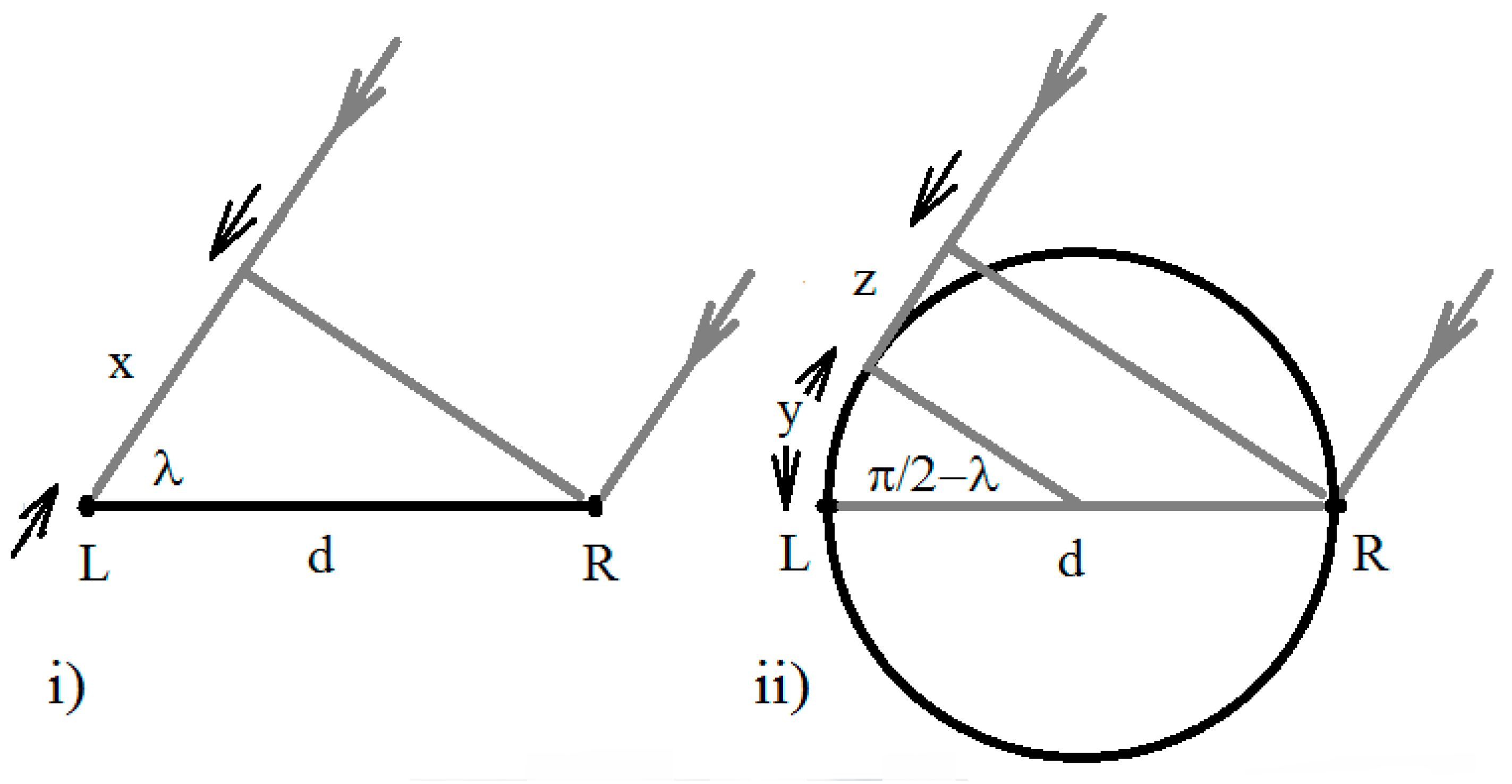
The angle between the direction to an acoustic source and the binaural auditory axis is the angle lambda ($\lambda$). Relationships between lambda ($\lambda$) and the time delay between signals received by a pair of listening antennae are illustrated in Figure 1 for two simple geometrical configurations of antennae on a head.

In Figure 1, L represents the position of the left antenna (ear), R the position of the right antenna and LR the line between the antennae on the auditory axis.

For antennae at the ends of a line (Figure 1i):

$$x=d\cos \lambda$$

(1)

$$\Delta t=\frac{x}{v}$$

(2)

$$\Delta t=\frac{d}{v}\cos \lambda$$

(3)

$$\lambda =\mathrm{acos}\left(\frac{v}{d} \Delta t\right)$$

(4)

and for antennae on opposite sides of a spherical head (e.g., [6,32]) (Figure 1ii):

$$y=\frac{d}{2} \left(\frac{\pi }{2}-\lambda \right)$$

(5)

$$z=\frac{d}{2} \cos \lambda$$

(6)

$$\Delta t=\frac{y+z}{v}$$

(7)

$$\Delta t=\frac{d}{2 v}\left(\cos \lambda +\frac{\pi }{2}-\lambda \right)$$

(8)

$$\cos \lambda -\lambda +\frac{\pi }{2}=\frac{2 v}{d} \Delta t$$

(9)

for which:

• $d$ is the distance between the listening antennae (ears); the length of the line LR,
• $\lambda$ is the angle between the auditory axis right of the head and the direction to the acoustic source,
• $\Delta t$ is the inter-aural time delay (ITD); the difference between arrival times at the antennae, and
• $v$ is the acoustic transmission velocity.

Equations (3) and (8) are employed to compute time delays $\Delta t$ for values of lambda $\lambda$. Equations (4) and (9) may be used to compute values of $\lambda$ from values of $\Delta t$. Equation (9) requires numerical solution or interpolation between values generated for a lookup table. These relationships are used to generate simulated data in later sections of the paper. In a real robotic system involving more complicated head geometries than those illustrated in Figure 1, for example, in a less approximate emulation of the human head, relationships between $\Delta t$ and $\lambda$ (and also elevation angle) may be established by direct measurement in control conditions.

3. Relationships between Signals Received at the Antennae

This section begins with an exploration of how the delay time $\Delta t$ and potentially other values from which the angle lambda between the line to an acoustic source and the auditory axis could be computed, might be extracted from signals received at the left and right antennae. The section then continues with an illustration of how acoustic amplitudes associated with time delays for multiple acoustic sources extracted at an effective instant in time (for a particular orientation of the head) can be represented in an instantaneous acoustic image of the field of audition.

3.1. Binaural Transfer Function

A complex transfer function (or admittance function) $Z$, computed from signals received at a pair of antennae (ears) would constitute a Fourier domain description of the relationship between the signals.

The complex transfer function could be computed from:

$$Z\left(k\right)=\frac{F\left(k\right)}{N\left(k\right)}$$

(10)

$$k=2\pi /\sigma$$

(11)

where:

• $F$ is the Fourier transform of the signal received by the antenna farther from an acoustic source,
• $N$ the Fourier transform of the signal received by the antenna nearer to the source,
• $k$ is the wavenumber, and
• $\sigma$ is wavelength (seconds).

The quantity $Z$ is the ratio of the amplitude of the signal received by the antenna farther from an acoustic source to the amplitude of the signal received by the antenna nearer the source as a function of wavenumber $k$. Two functions would need to be computed, one for sources of sound in the hemisphere to the right side of the median plane between the antennae and one for acoustic sources left of the median plane. The shape of the amplitude response function for a particular acoustic source would be related to the angle lambda. A relationship between $Z\left(k\right)$ amplitudes and lambda $\lambda$ would need to be extracted empirically employing an independent means for estimating $\lambda$. For short ranges (relative to the distance between the antennae) the relationship is likely to be rendered more complicated by the effect of short range on inter-aural level differences [21] and therefore $Z\left(k\right)$ amplitude values. A relationship between $Z\left(k\right)$ amplitude and lambda $\lambda$ once elucidated would allow values of lambda to be determined independently of ITD values.

An inversion of $Z\left(k\right)$ from the Fourier domain to its equivalent in the time domain $z\left(t\right)$ represents the filter that convolved with the signal received by the antenna nearer to an acoustic source $n\left(t\right)$ would generate the signal received by the antenna farther from the source $f\left(t\right)$. It would contain information on time delays between signals arriving at the ears and so provide a complementary approach to computing values for lambda that does depend on ITD values.

3.2. Binaural Cross-Correlation Function

Less generally but perhaps more intuitively, time delay data can be extracted from a short-time base cross correlation function $x\left(\Delta t\right)$ [33] of signal received by the right hand and the left hand antennae at a time $t=t_0$.

Consider two time series recorded by the right side antenna $s\left(t\right)$ ($s$ for starboard) and the left side antenna $p\left(t\right)$ ($p$ for port). A short-time base cross correlation function (CCF) of the signal received at the antennae at the time $t=t_0$ may be expressed:

$$x\left(\Delta t\right)={{\displaystyle \int }}_{t=t_0-T/2}^{t=t_0+T/2}p\left(t\right) s\left(\Delta t+t\right) dt$$

(12)

$$-c d/v \le \Delta t \le c d/v$$

$$T>4c d/v$$

where:

• $\Delta t$ is the variable representing arrival time differences between antennae,
• $T$ is the length of the short-time base of the cross correlation function, and
• $c$ is a constant; being the ratio of the maximum inter-aural ray path length difference

(when $\lambda$ = 0° or 180°) to the distance between the antennae.

The value of the constant $c$ is 1 for antennae disposed along a line and (1 + $\pi$/2)/2 = 1.285 for antennae disposed on opposite sides of a spherical head. The factor 4 is present in the inequality for the time base length $T$ to provide an appropriate overlap in the time series $p$ and $s$ at the extremities for the value of $t$ in the integral for computing the CCF.

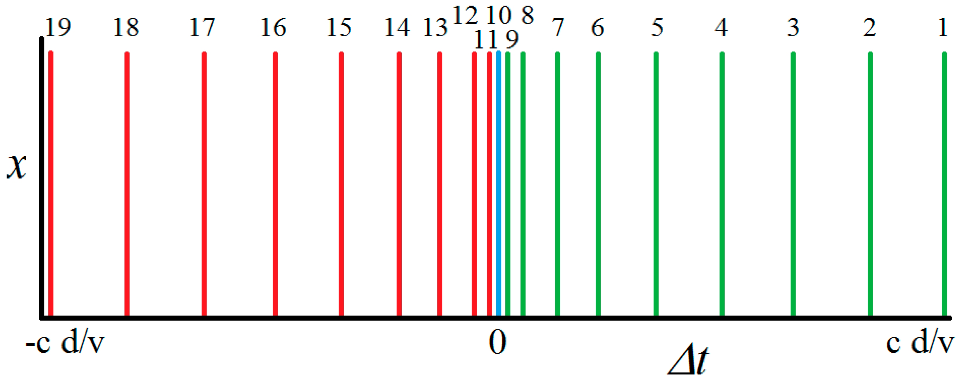
A CCF at an effectively instantaneous time $t_0$ (for a given orientation of the head) is illustrated schematically in Figure 2 for hypothetical multiple acoustic sources. The CCF coefficients can be represented in an acoustic image of the field of audition in a manner illustrated in Figure 3 for which details are provided in

Table 1. Values of lambda $\lambda$ spaced at 10° intervals over a 180° range. Corresponding arrival time differences $\Delta t$ (illustrated schematically in Figure 1) for antennae disposed at the ends of a line are tabulated in column 3 (Equation (3)) and for antennae on the sides of a spherical head in column 4 (Equation (8)). The loci of 19 lambda circles along which cross-correlation function coefficients would be distended in an acoustic image of the field of audition are shown for a non-sloping auditory axis in Figure 3i and for an auditory axis sloping to the right across the head $i$ = 20° in Figure 3ii.

Circle	$\mathit{\lambda }$	$\mathit{\Delta }\mathit{t} \left(\mathbf{Line}\right)$	$\mathit{\Delta }\mathit{t} \left(\mathbf{Sphere}\right)$
1	0°	437 μs	560 μs
2	10°	431 μs	521 μs
3	20°	411 μs	473 μs
4	30°	379 μs	418 μs
5	40°	335 μs	358 μs
6	50°	281 μs	293 μs
7	60°	219 μs	223 μs
8	70°	150 μs	151 μs
9	80°	75.8 μs	76.1 μs
10	90°	0 μs	0 μs
11	100°	−75.8 μs	−76.1 μs
12	110°	−150 μs	−151 μs
13	120°	−219 μs	−223 μs
14	130°	−281 μs	−293 μs
15	140°	−335 μs	−358 μs
16	150°	−379 μs	−418 μs
17	160°	−411 μs	−473 μs
18	170°	−431 μs	−521 μs
19	180°	−437 μs	−560 μs

.

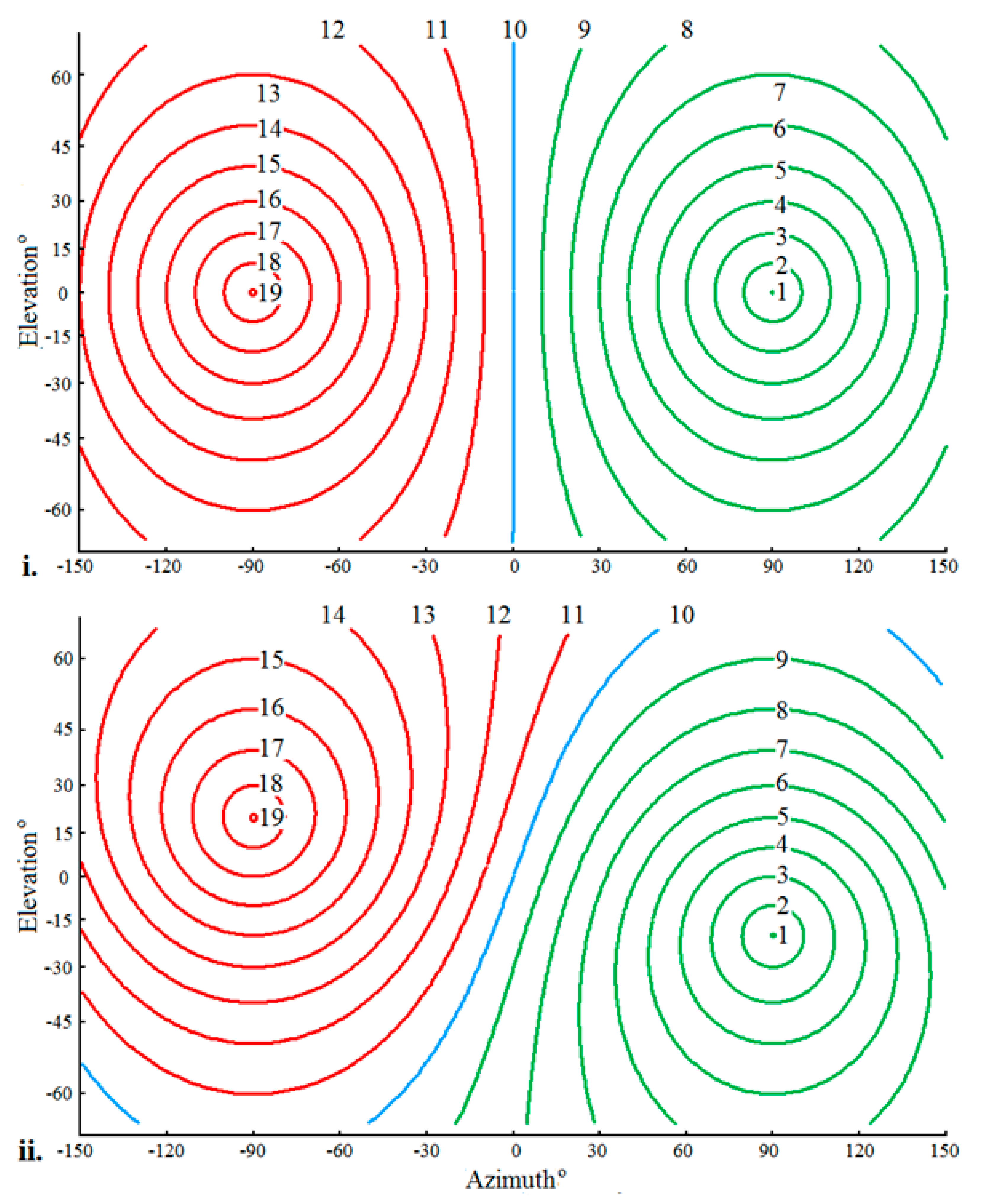
Figure 2 illustrates schematically the form of a hypothetical CCF for nineteen acoustic sources disposed around the hemisphere in front of a face at bearings with a constant interval of 10°. It is most unlikely that so many acoustic sources could be independently recognized in a CCF. One of the limitations of simulated rather than real data is that the problem of disentangling sound from multiple acoustic sources can be glossed over. For multiple sources to generate distinguishable events in a CCF the sources would need to have sufficiently different spectral characteristics. Where sources have very different spectral characteristics, for example the different instruments in an orchestra, this would be expected to be relatively easy and perhaps up to 19 different instruments playing simultaneously could be distinguished. The problem is more challenging however where differences in spectral characteristics are subtler, for example as encountered where multiple humans are speaking simultaneously. The purpose of Figure 2 and Figure 3 and Table 1 based on simulated data is to illustrate how a CCF’s coefficients can in principle be represented in an acoustic image of the field of audition.

The simulated data in Table 1 are computed for nineteen lambda circles (Figure 3) corresponding to acoustic sources identified with peaks in the CCF shown schematically in Figure 2. Delay time data are computed for antennae disposed at the ends of a line (Equation (3)) and for antennae disposed to the sides of a spherical head (Equation (8)) ($v$ = 343 m/s, $d$ = 0.15 m).

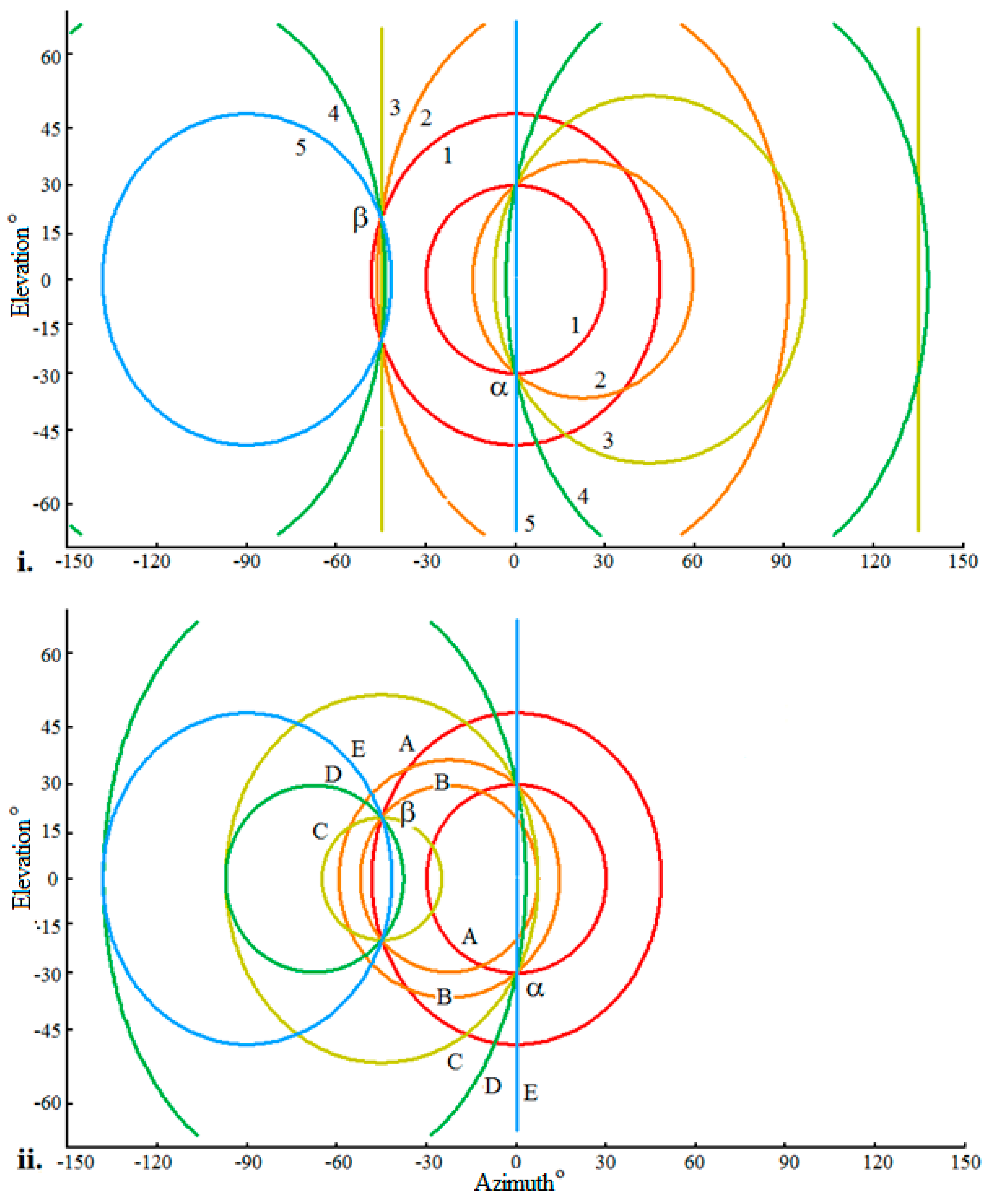
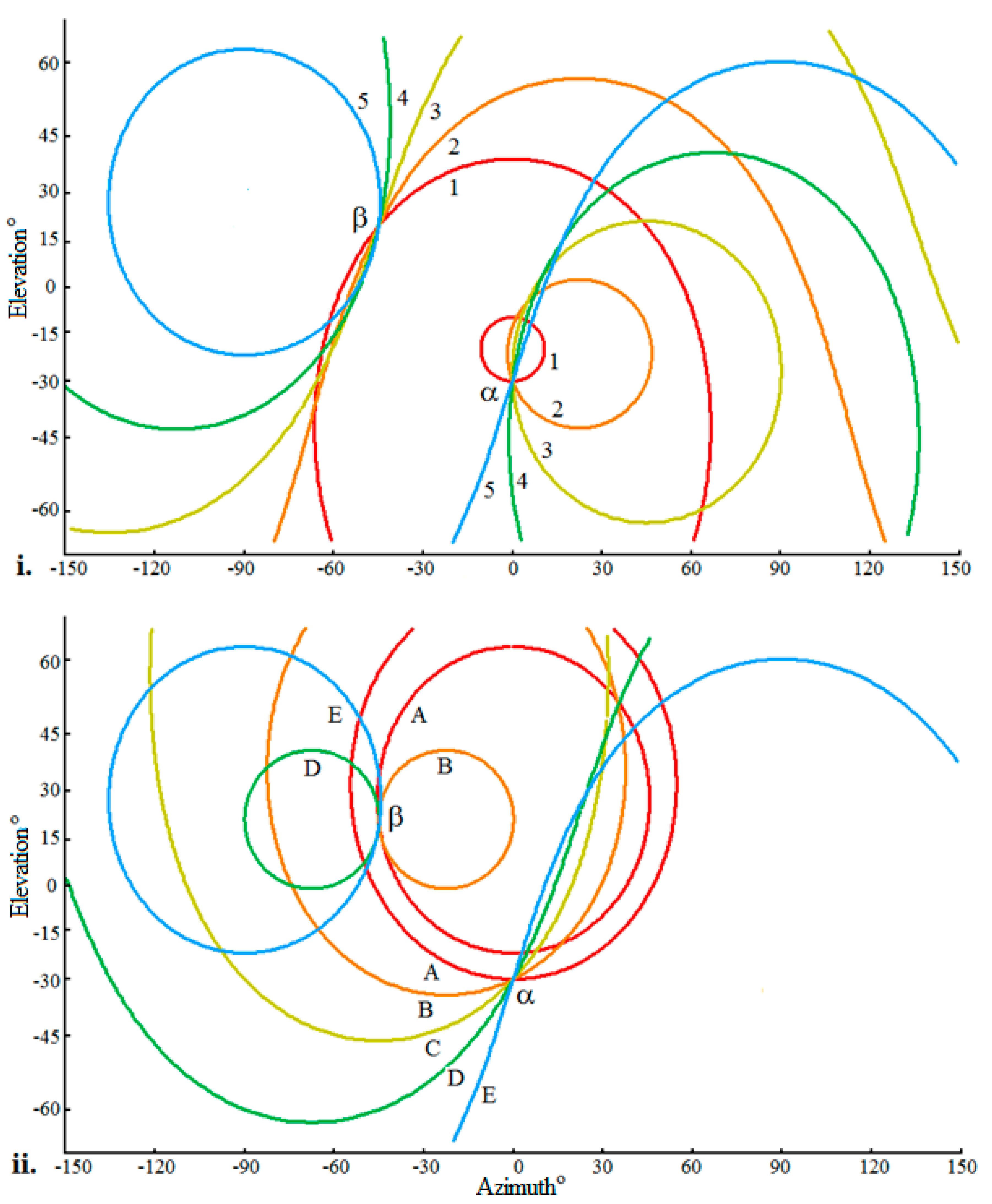
The lambda circles shown in Figure 3 are the loci along which CCF coefficients associated with the data in Table 1 would be distended to form an acoustic image of the field of audition corresponding to the short-time base CCF illustrated schematically in Figure 2. Data at peaks in the CCF would be distended over corresponding lambda circles. Circles are shown in Figure 3 for two orientations of the auditory axis on the head. Figure 3i shows circles for the case of a horizontal auditory axis. Figure 3ii is for the case of the auditory axis sloping to the right across the head at an angle of $i$ = 20° in emulation of a feature of the auditory systems of species of owl [34,35,36,37]. The lambda circles for a horizontal auditory axis are symmetric about the horizontal (zero elevation) whereas the lambda circles for an inclined axis are symmetric about an inclined great circle passing through the point azimuth = 0°, elevation = 0°.

The principal feature of a set of lambda circles corresponding to acoustic sources in an instantaneous acoustic image of the field of audition for a given orientation of the head (Figure 3) is that the circles all share a common polar axis.

3.3. Head Related Transfer Function

The human auditory system appears to be capable of extracting transfer functions not only that encapsulate the relationship between signals incident at the left and right ears but also between signal incident at the ears and signal approaching the head but not recorded in any way. The head and the external ears (pinnae) affect the spectral characteristics of data transduced at the ears. In particular spectra are found to have characteristic notches and to a lesser extent characteristic maxima [26]. Remarkably the human auditory system would appear to be able to infer angular elevation to acoustic sources from such spectral characteristics. This process operates on high frequency signal incident on the ears (>1500 Hz) [38,39] but apparently not on signal at lower frequencies, most likely due to higher frequency signal being more susceptible to diffraction around the head and pinnae. The auditory system must be able to extract a HRTF during a training process by relating characteristics of signals received at the ears to the locations of acoustic sources determined by a means independent of the HRTF. It is possible that a HRTF in humans is to some extent innate and that a training process fine tunes the transfer function. A fuller consideration of HRTFs is outside of the scope of this paper.

4. Multiple Acoustic Source Synthetic Aperture Audition

An integration of many short-time base effectively instantaneous acoustic images into a mid-time base acoustic image of the field of audition as the head is turned constitutes a synthetic aperture computation (SAC) [19] and is the subject of this section.

Data in an acoustic image of the field of audition corresponding to the coefficients in a short-time base instantaneous binaural CCF may be integrated in an acoustic image of the field of audition maintained for sufficient time to integrate data as the head is turned (up to say approximately 0.5 s).

Between computations of short-time base effectively instantaneous CCFs the head is rotated through an angle ($\Delta {\theta }_H$, $\Delta {\varphi }_H$, $\Delta i_H$); the components of rotation about three orthogonal axes: the head’s vertical axis (a turn); the axis across the head (a nod); and the axis in the direction in which the head is facing (a tilt). The data stored in the mid-time base acoustic image of the field of audition are rotated by ($-\Delta {\theta }_H$, $-\Delta {\varphi }_H$, $-\Delta i_H$) in order that the content of the mid-time base acoustic image remains static relative to the real world as the orientation of the head changes. The coefficients in the current short-time base CCF distended over lambda circles in the instantaneous acoustic image of field of audition are then integrated (added) into the mid-time base acoustic image. The CCF coefficients being the product of two amplitudes are a measure of energy/power and therefore suitable for integration by simple addition into the mid-time base acoustic image. The SAC is analogous to the computation performed in the process of migration applied to raw seismic profiler data and in synthetic aperture side scan sonar/radar data processing [19,40].

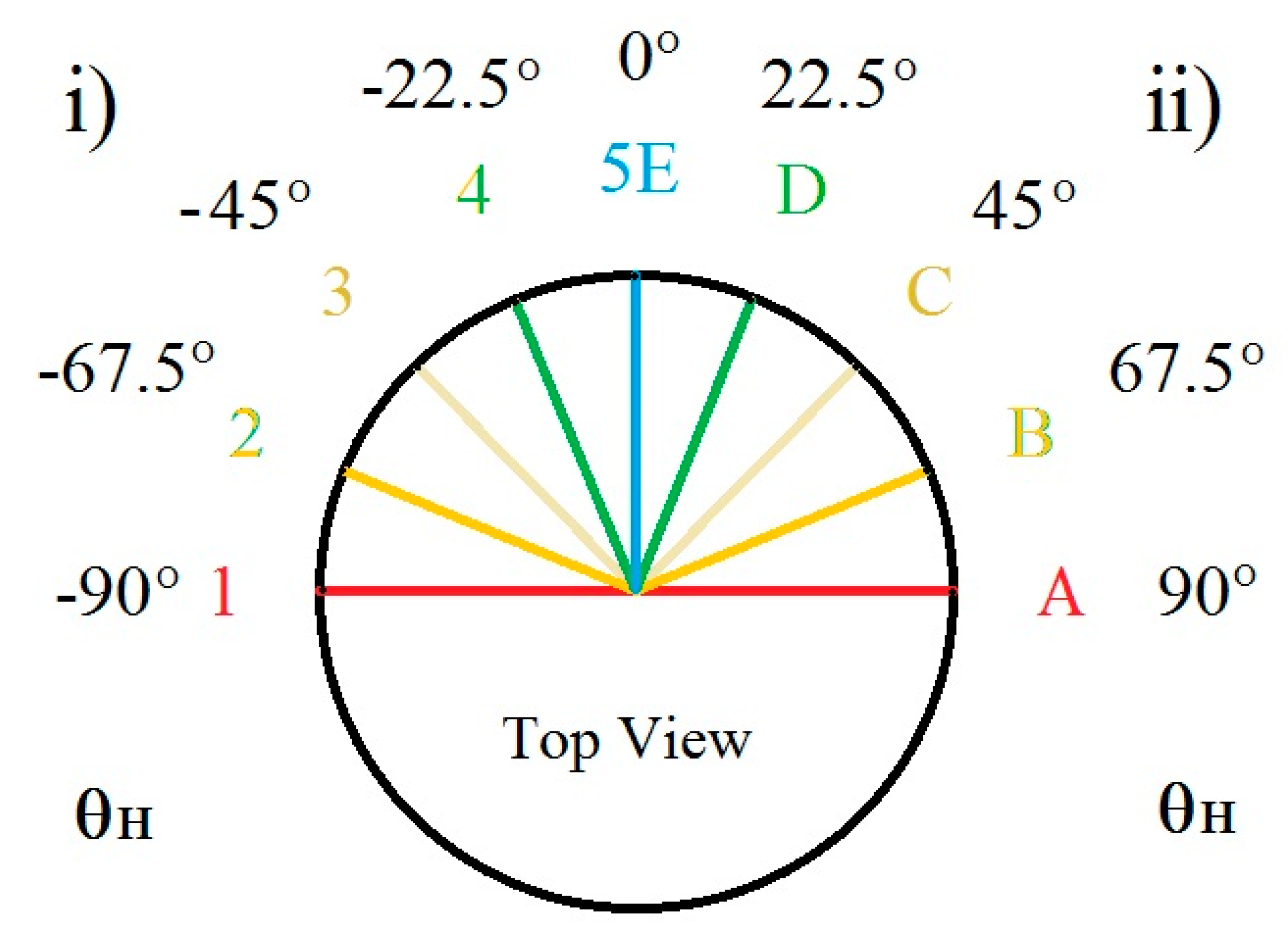
Lambda circles for multiple acoustic sources, after integration into an image of the field of audition as the head is turned, are illustrated in

Table 2. Simulated values of lambda $\lambda$ for the circles shown in Figure 5 for a horizontal auditory axis for two acoustic sources $\mathsf{\alpha }$ and $\mathsf{\beta }$ computed for bearings of the head ${\theta }_H$ (Figure 4) at 22.5° intervals (red to blue). Values of inter-aural time delay (ITD) $\Delta t$ are computed using Equations (3) and (8) ($v$ = 343 m/s, $d$ = 0.15 m).

Figure Circle	$\mathbf{Bearing} {\mathit{\theta }}_{\mathit{H}}$	$\mathsf{\alpha }: \mathit{\lambda }$	$\mathsf{\alpha }: \mathit{\Delta }\mathit{t} \left(\mathbf{Line}\right)$	$\mathsf{\alpha }: \mathit{\Delta }\mathit{t} \left(\mathbf{Sphere}\right)$	$\mathsf{\beta }: \mathit{\lambda }$	$\mathsf{\beta }: \mathit{\Delta }\mathit{t} \left(\mathbf{Line}\right)$	$\mathsf{\beta }: \mathit{\Delta }\mathit{t} \left(\mathbf{Sphere}\right)$
5i.1	−90.0°	30.0°	379 μs	418 μs	28.3°	291 μs	304 μs
5i.2	−67.5°	35.9°	350 μs	378 μs	68.9°	157 μs	159 μs
5i.3	−45.0°	52.2°	268 μs	278 μs	90.0°	0 μs	0 μs
5i.4	−22.5°	70.6°	145 μs	146 μs	111.1°	−157 μs	−159 μs
5i.55ii.E	0.0°	90.0°	0 μs	0 μs	131.6°	−291 μs	−304 μs
5ii.D	22.5°	109.3°	−145 μs	−146 μs	150.2°	−380 μs	−420 μs
5ii.C	45.0°	127.8°	−268 μs	−278 μs	160.0°	−411 μs	−473 μs
5ii.B	67.5°	143.1°	−350 μs	−378 μs	150.2°	−380 μs	−420 μs
5ii.A	90.0°	150.0°	−379 μs	−418 μs	131.6°	−291 μs	−304 μs

and Figure 5 for an uninclined auditory axis. Similarly, lambda circles are shown in

Table 3. Simulated values of lambda $\lambda$ for the circles in Figure 6 for an auditory axis inclined across the head to the right at $i$ = 20° for two acoustic sources $\mathsf{\alpha }$ and $\mathsf{\beta }$ computed for bearings of the head ${\theta }_H$ (Figure 4) at 22.5° intervals (red to blue). Values of inter-aural time delay (ITD) $\Delta t$ are computed using Equations (3) and (8) ($v$ = 343 m/s, $d$ = 0.15 m).

Figure Circle	$\mathbf{Bearing} \mathit{\theta }$	$\mathsf{\alpha }: \mathit{\lambda }$	$\mathsf{\alpha }: \mathit{\Delta }\mathit{t} \left(\mathbf{line}\right)$	$\mathsf{\alpha }: \mathit{\Delta }\mathit{t} \left(\mathbf{sphere}\right)$	$\mathsf{\beta }: \mathit{\lambda }$	$\mathsf{\beta }: \mathit{\Delta }\mathit{t} \left(\mathbf{line}\right)$	$\mathsf{\beta }: \mathit{\Delta }\mathit{t} \left(\mathbf{sphere}\right)$
6i.1	90.0°	10.0°	431 μs	521 μs	59.5°	222 μs	227 μs
6i.2	67.5°	22.6°	404 μs	459 μs	77.2°	97 μs	97 μs
6i.3	45.0°	41.7°	326 μs	347 μs	96.7°	−51 μs	−51 μs
6i.4	22.5°	61.2°	211 μs	216 μs	117.1°	−199 μs	−203 μs
6i.56ii.E	0.0°	80.1°	75 μs	75 μs	137.8°	−324 μs	−345 μs
6ii.D	−22.5°	98.1°	−61 μs	−62 μs	158.9°	−408 μs	−469 μs
6ii.C	−45.0°	113.9°	−177 μs	−179 μs	180.0°	−437 μs	−560 μs
6ii.B	−67.5°	125.5°	−254 μs	−263 μs	158.9°	−408 μs	−469 μs
6ii.A	−90.0°	130.0°	−281 μs	−293 μs	137.8°	−324 μs	−345 μs

and Figure 6 for the case of an auditory axis inclined to the right across the head at $i$ = 20° (in emulation of species of owl). Simulated delay time data for two acoustic sources, one 30° below the horizontal and one 20° above it and separated azimuthally by 45° are shown: i. in the top halves of Table 2 and Table 3 for five instances in time as the head is turned from facing 90° to the left to looking straight ahead and similarly; ii. in the lower halves of Table 2 and Table 3 for five instances in time as the head is turned from facing 90° to the right to looking straight ahead (see Figure 4).

Values for $\lambda$ in columns 3 and 6 of Table 2 and Table 3 are computed as a function of angles between the directions to acoustic sources with respect to the direction the head is facing ($\theta$, $\phi$ and $i$) [19] from:

$$\lambda =acos\left(\mathit{sin}\theta \mathit{cos}i\mathit{cos}\phi +\mathit{sin}i\mathit{sin}\phi \right)$$

(13)

where:

• $\theta$ is the azimuth (longitudinal) angle to an acoustic source to the right of the direction in which the head is facing,
• $\phi$ is the elevation (latitudinal) angle below the horizontal (with respect to the direction the head is facing) to an acoustic source, and
• $i$ is the inclination of the auditory axis to the right across the head.

Figure 5 and Figure 6 represent images of the field of audition in Mercator projection showing collections of lambda small circles of colatitude for just five instances in time while the head is turned about a vertical axis through 90°. In a real system, at least an order of magnitude more instantaneous CCFs would be required. Just five are shown in Figure 5 and Figure 6 for the purpose of illustration and not to overcharge the figures with an excess of detail.

Similarly, lambda circles for just two acoustic sources are shown in Figure 5 and Figure 6 to illustrate the principle upon which multiple acoustic sources can simultaneously be located without overwhelming the figures with detail.

In each of the graphs in Figure 5 and Figure 6, lambda circles with the same colour represent the same instant in time (and the same orientation of the head) but different acoustic sources. Like the lambda circle plots in Figure 3, circles with the same colour in the plots in Figure 5 and Figure 6 share a polar axis. One of the yellow lambda circles occupies a point coincident with the acoustic source above the horizon in Figure 6ii and therefore cannot be seen.

Lambda circles having different colours form sets that converge at common points corresponding to the locations of the acoustic sources. However, in Figure 5 for which the auditory axis is horizontal, there is symmetry about the horizontal (an elevation of 0°) and the locations of the acoustic sources are not uniquely located. This arises because in rotating the head about its vertical axis (for ${\varphi }_H$ = 0 and $i_H$ = 0) the auditory axis occupies always the same plane. In contrast, in Figure 6 for which the auditory axis slopes across the head to the right at $i$ = 20° it is seen that the acoustic sources are uniquely located. The plane in which a sloping auditory axis lays continuously changes as the head is turned about its vertical axis and so acoustic sources are located unambiguously. Thus, a sloping auditory axis confers a distinct advantage that appears to have been successfully exploited through evolution by species of owls better equipping them to locate prey in low or zero light conditions using audition alone [34,35,36,37].

5. Discussion

Peaks in the coefficients of a short-time base (of the order >2.25 milliseconds) CCF between signals arriving at the left and right antennae $x\left(\Delta t\right)$ represent the registration of acoustic sources at effectively an ‘instant’ in time for a particular orientation of the head. These coefficients being a function of delay time $\Delta t$ can also be expressed as a function of $\lambda$ by computing values of $\lambda$ from values of $\Delta t$ using Equation (4) for antennae disposed along a line and solving for Equation (9) for antennae disposed either side of a spherical head. For simple geometrical arrangements of antennae on a head such as those illustrated in Figure 1 an analytic relationship between time delay and lambda may be readily computed. For more complex arrangements in binaural robotic systems, more generally the relationship between time delay and lambda can be established by direct measurement in control conditions.

A minimum short-time base length for a short-time base CCF, $T=4c d/v$, is approximately 2250 μs (2.25 ms) for a spherical head of diameter 0.15m. If the head takes up to say 0.5 seconds to turn from right to left or vice versa then this would provide an appropriate maximum duration for the mid-time base for a SAC, and sufficient time for the results of up to a little over 220 CCFs to be integrated into a mid-time base acoustic image. Allowing a 50% overlap at the ends of the CCF time base between computations, this doubles to 440 CCFs. If a CCF is computed for every 0.25° turned by the head, then $N$ for a 90° turn of the head would be 360 (a CCF rate of 720 Hz) and this number of CCFs can be comfortably accommodated to enable a mid-time base acoustic image with sufficient resolution to determine the locations of acoustic targets to better than a degree in azimuth and elevation. Increasing the length of the CCF time base and reducing the rate at which CCFs are computed as the head is turned will lower the achievable resolution of acoustic source localization but would permit longer acoustic wavelengths to be included in the CCF calculation.

The mid-time base acoustic image of the field of audition generated in performing a SAC would need to be explored by a higher-level function designed to locate bright (high amplitude) points in the SAC mid-time base acoustic image and possibly pick up other characteristics of signal associated with the bright point. This information could then be registered in a persistent long-time base acoustic image of the field of audition representing the robot’s acoustic environmental world view. The duration of the long-term time base might extend to multiple tens of seconds. Information in the current mid-time base SAC acoustic image could be compared with that in the long-time World View acoustic image and the information in the latter updated and overridden if the quality of the data in the SAC image is superior to that in the World View image. In this way a process of collating the information in acoustic images of the field of audition generated and maintained for the wide range of time base lengths can generate and maintain a persistent long-term acoustic image of the location and character of multiple acoustic sources in the field of audition of a binaural robot.

A limitation of the current paper is the absence of data from an implementation of the method in a real world binaural robotic system to support the description of the method based on simulated data. Whilst it is hoped that in the course of time this will be rectified some mention at least should be made of the challenges likely to be encountered with real data that do not affect the simulated data. One is that it has been assumed in generating simulated data that acoustic sources are stationary. This is not an overwhelming limitation because the angular speed of acoustic sources across the robot’s field of audition while performing a SAC will usually be considerably less than the angular speed of rotation of the robot’s head. How the SAC process might be adjusted for localizing fast moving sources is not considered further here.

Another issue affecting real world binaural systems is the deleterious effect of reverberation on acoustic source localization. Sounds reflecting from flat surfaces and scattering from objects are likely to lead to spurious ITD events in CCFs for example. It is conjectured that the SAC process might enjoy some immunity to this problem because for an acoustic source to register in a SAC acoustic image it must be identified multiple times for example, in multiple CCFs, and the lambda circles for the events must coherently intersect at points in the SAC acoustic image. It is unlikely that spurious events arriving from different directions will coherently integrate to generate ‘bight spots’ at points in the SAC image.

Uncertainty also impacts real data whilst the simulated data are essentially noise free. Sources of uncertainty in real data include a systematic error in the assumed value of the acoustic transmission speed leading to bias in the values of lambda computed from ITDs and random errors in the values of ITDs extracted from CCFs. The effect of such uncertainties is that lambda circles in SAC acoustic images of the field of audition will intersect within areas rather than at points. The SAC images may be exploited to extract information on the extent of such areas in the images to provide data on uncertainties in azimuth and elevation of the locations of acoustic sources.

There is a potential role for the SAC process in calibrating a binaural robot’s HRTF. In providing estimates of acoustic source locations in azimuth and elevation independent of that provided through use of a HRTF, information derived from the SAC process could be deployed for the purpose of training the HRTF. As a matter of conjecture this might be a feature of natural binaural systems but whether it is or not, it could be deployed to train a HRTF based localization process in a binaural robotic system.

6. Summary

A binaural robot can extract effectively instantaneous inter-aural time delay (ITD) data for acoustic events arriving at the listening antennae from multiple acoustic sources by, for example, computing cross-correlation functions (CCFs) from short-time base time series incident at the antennae. Such time series would require a minimum time base duration of four times the maximum possible inter-aural delay between the antennae. The coefficients of the CCF may be distended over lambda circles in an acoustic image of the field of audition to represent in image form the information inherent in ITDs at an effective instant in time for a particular orientation of the head. The key feature of lambda circles for multiple acoustic sources acquired for the same instant in time is that they share a common polar axis.

As the head is turned, acoustic images generated for instantaneous measurements of ITDs are integrated in a mid-time base acoustic image of the field of audition, the length of the mid-time base being of the order of the time it takes to turn the head (up to say 0.5 seconds). Points in the integrated image of the field of audition at which lambda circles converge and intersect produce bright spots or maxima in the image and the positions of these in the image correspond to the locations of acoustic sources. Thus, the two listening antennae of a binaural robot can extract information on directions to multiple acoustic sources over a spherical field of audition from a process of integration constituting a synthetic aperture computation (SAC) similar in its essentials to the process of migration performed on seismic profiler data and in synthetic aperture computation in synthetic aperture sonar and radar. This SAC process satisfies the criteria for the ‘dynamic’ process inferred by Wallach [13] performed by the human auditory system to overcome the ambiguity in the direction to an acoustic source inherent in a single instantaneous lambda circle, by integrating information while listening to a sound as the head is turned. This article has been principally concerned with the fundamentals of the mid-time base process of generating a SAC image of the field of audition

The SAC image of the field of audition may subsequently be subjected to a higher-level process to extract information from the image and compare it to information stored in a long-term persistent image of the field of audition constituting the robot’s aural environmental world view. Provided data quality criteria of events in the current SAC image exceed those of data already held in the world view, information may be copied into the world view from that derived from the SAC image.

The acoustic images of the field of audition over the range of timescales discussed in the article are inherently visual and a robotic system could be provided with an option to display the acoustic images on external monitors for human visualization of the processing of the data and of the results extracted. This would provide a wealth of information to engineers for the purposes of debugging the system and for suggesting new ideas for ongoing system development.

References

- Lollmann, H.W.; Barfus, H.; Deleforge, A.; Meier, S.; Kellermann, W. Challenges in acoustic signal enhancement for human-robot communication. In Proceedings of the ITG Conference on Speech Communication, Erlangen, Germany, 24–26 September 2014. [Google Scholar]
- Takanishi, A.; Masukawa, S.; Mori, Y.; Ogawa, T. Development of an anthropomorphic auditory robot that localizes a sound direction. Bull. Centre Inform. 1995, 20, 24–32. (In Japanese) [Google Scholar]
- Voutsas, K.; Adamy, J. A biologically inspired spiking neural network for sound source lateralization. IEEE Trans. Neural Netw. 2007, 18, 1785–1799. [Google Scholar] [CrossRef] [PubMed]
- Liu, J.; Perez-Gonzalez, D.; Rees, A.; Erwin, H.; Wermter, S. A biologically inspired spiking neural network model of the auditory midbrain for sound source localization. Neurocomputing 2010, 74, 129–139. [Google Scholar] [CrossRef]
- Sun, L.; Zhong, X.; Yost, W. Dynamic binaural sound source localization with interaural time difference cues: Artificial listeners. J. Acoust. Soc. Am. 2015, 137, 2226. [Google Scholar] [CrossRef]
- Kim, U.H.; Nakadai, K.; Okuno, H.G. Improved sound source localization in horizontal plane for binaural robot audition. Appl. Intell. 2015, 42, 63–74. [Google Scholar] [CrossRef]
- Nakadai, K.; Lourens, T.; Okuno, H.G.; Kitano, H. Active audition for humanoids. In Proceedings of the 17th National Conference Artificial Intelligence (AAAI-2000), Austin, TX, USA, 30 July–3 August 2010; pp. 832–839. [Google Scholar]
- Cech, J.; Mittal, R.; Delefoge, A.; Sanchez-Riera, J.; Alameda-Pineda, X. Active speaker detection and localization with microphone and cameras embedded into a robotic head. In Proceedings of the IEEE-RAS International Conference on Humanoid Robots (Humanoids), Atlanta, GA, USA, 15–17 October 2013; pp. 203–210. [Google Scholar]
- Nakamura, K.; Nakadai, K.; Asano, F.; Ince, G. Intelligent sound source localization and its application to multimodal human tracking. In Proceedings of the IEEE/RSJ International Conference on Intelligent Robots and Systems, San Francisco, CA, USA, 25–30 September 2011; pp. 143–148. [Google Scholar]
- Yost, W.A.; Zhong, X.; Najam, A. Judging sound rotation when listeners and sounds rotate: Sound source localization is a multisystem process. J. Acoust. Soc. Am. 2015, 138, 3293–3310. [Google Scholar] [CrossRef] [PubMed]
- Ma, N.; May, T.; Brown, G. Exploiting deep neural networks and head movements for robust binaural localization of multiple sources in reverberant environments. IEEE Trans. Audio Speech Lang. Process. 2017, 25, 2444–2453. [Google Scholar] [CrossRef]
- Rodemann, T.; Heckmann, M.; Joublin, F.; Goerick, C.; Scholling, B. Real-time sound localization with a binaural head-system using a biologically-inspired cue-triple mapping. In Proceedings of the IEEE/RSJ International Conference on Intelligent Robots and Systems, Beijing, China, 9–15 October 2006; pp. 860–865. [Google Scholar]
- Wallach, H. The role of head movement and vestibular and visual cues in sound localisation. J. Exp. Psychol. 1940, 27, 339–368. [Google Scholar] [CrossRef]
- Portello, A.; Danes, P.; Argentieri, S. Acoustic models and Kalman filtering strategies for active binaural sound localization. In Proceedings of the IEEE/RSJ International Conference on Intelligent Robots and Systems, San Francisco, CA, USA, 25–30 September 2011; pp. 137–142. [Google Scholar]
- Zhong, X.; Sun, L.; Yost, W. Active binaural localization of multiple sound sources. Robot. Auton. Syst. 2016, 85, 83–92. [Google Scholar] [CrossRef]
- Gala, D.; Lindsay, N.; Sun, L. Three-dimensional sound source localization for unmanned ground vehicles with a self-rotational two-microphone array. In Proceedings of the 5th International Conference of Control, Dynamic Systems and Robotics, Niagara Falls, ON, Canada, 7–9 June 2018; pp. 104–111. [Google Scholar]
- Lee, S.; Park, Y.; Park, Y. Three-dimensional sound source localization using inter-channel time difference trajectory. Int. J. Adv. Robot. Syst. 2015, 12, 171. [Google Scholar] [CrossRef]
- Long, T.; Chen, J.; Huang, G.; Benesty, J.; Cohen, I. Acoustic source localization based on geometric projection in reverberant and noisy environments. IEEE J. Sel. Top. Signal Process. 2018. [Google Scholar] [CrossRef]
- Tamsett, D. Synthetic aperture computation as the head is turned in binaural direction finding. Robotics 2017, 6, 3. [Google Scholar] [CrossRef]
- Winter, F.; Schultz, S.; Spors, S. Localisation properties of data-based binaural synthesis including translator head-movements. In Proceedings of the Forum Acusticum, Krakow, Poland, 7–12 September 2014. [Google Scholar]
- Magassouba, A.; Bertin, N.; Chaumette, F. Exploiting the distance information of the interaural level difference for binaural robot motion control. IEEE Robot. Autom. Lett. 2018, 3, 2048–2055. [Google Scholar] [CrossRef]
- Tamsett, D. Binaural Range Finding from Synthetic Aperture Computation as the Head is Turned. Robotics 2017, 6, 10. [Google Scholar] [CrossRef]
- Perrett, S.; Noble, W. The effect of head rotations on vertical plane sound localization. J. Acoust. Soc. Am. 1997, 102, 2325–2332. [Google Scholar] [CrossRef] [PubMed]
- Roffler, S.K.; Butler, R.A. Factors that influence the localization of sound in the vertical plane. J. Acoust. Soc. Am. 1968, 43, 1255–1259. [Google Scholar] [CrossRef] [PubMed]
- Batteau, D. The role of the pinna in human localization. Proc. R. Soc. Lond. B Biol. Sci. 1967, 168, 158–180. [Google Scholar] [PubMed]
- Blauert, J. Spatial Hearing—The Psychophysics of Human Sound Localization; The MIT Press: Cambridge, MA, USA; London, UK, 1983; p. 427. [Google Scholar]
- Middlebrooks, J.C.; Makous, J.C.; Green, D.M. Directional sensitivity of sound-pressure levels in the human ear canal. J. Acoust. Soc. Am. 1989, 86, 89–108. [Google Scholar] [CrossRef]
- Shimoda, T.; Nakashima, T.; Kumon, M.; Kohzawa, R.; Mizumoto, I.; Iwai, Z. Sound localization of elevation using pinnae for auditory robots. In Robust Speech Recognition and Understanding; Grimm, M., Kroschel, K., Eds.; I-Tech: Vienna, Austria, 2007; p. 460. ISBN 987-3-90213-08-0. [Google Scholar]
- Rodemann, T.; Ince, G.; Joublin, F.; Goerick, C. Using binaural and spectral cues for azimuth and elevation localization. In Proceedings of the IEEE/RSJ International Conference on Intelligent Robots and Systems, Nice, France, 22–26 September 2008; pp. 2185–2190. [Google Scholar]
- Mironovs, M.; Lee, H. Vertical amplitude panning for various types of sound sources. In Proceedings of the Interactive Audio Systems Symposium, York, UK, 23 September 2016; pp. 1–5. [Google Scholar]
- Kohnen, M.; Bomhardt, J.; Fels, J.; Vortander, M. Just noticeable notch smoothing of head-related transfer functions. In Proceedings of the Fortschritte der Akustik—DAGA 2018: 44. Jahrestagung fur Akustik, Munich, Germany, 19–22 May 2018. [Google Scholar]
- Stern, R.; Brown, G.J.; Wang, D.L. Binaural sound localization. In Computational Auditory Scene Analysis; Wang, D.L., Brown, G.L., Eds.; John Wiley and Sons: New York, NY, USA, 2005; pp. 1–34. [Google Scholar]
- Sayers, B.M.A.; Cherry, E.C. Mechanism of binaural fusion in the hearing of speech. J. Acoust. Soc. Am. 1957, 36, 923–926. [Google Scholar] [CrossRef]
- Knudsen, E.I.; Konishi, M. Mechanisms of sound localization in the barn owl (Tyto alba). J. Compar. Physiol. A 1979, 133, 13–21. [Google Scholar] [CrossRef]
- Bala, A.D.S.; Spitzer, M.W.; Takahashi, T.T. Prediction of auditory spatial acuity from neural images of the owl’s auditory space map. Nature 2003, 424, 771–774. [Google Scholar] [CrossRef] [PubMed]
- Martin, G.R. The Sensory Ecology of Birds, 1st ed.; Oxford University Press: Oxford, UK, 2017; p. 296. [Google Scholar]
- Krings, M.; Rosskamp, L.; Wagner, H. Development of ear asymmetry in the American barn owl (Tyto furcate pratincola). Zoology 2018, 126, 82–88. [Google Scholar] [CrossRef] [PubMed]
- Wightman, F.L.; Kistler, D.J. The dominant role of low frequency interaural time differences in sound localization. J. Acoust. Soc. Am. 1992, 91, 1648–1661. [Google Scholar] [CrossRef] [PubMed]
- Brughera, A.; Danai, L.; Hartmann, W.M. Human interaural time difference thresholds for sine tones: The high-frequency limit. J. Acoust. Soc. Am. 2013, 133, 2839–2855. [Google Scholar] [CrossRef] [PubMed]
- Lurton, X. Seafloor-mapping sonar systems and Sub-bottom investigations. In An Introduction to Underwater Acoustics: Principles and Applications, 2nd ed.; Springer: Berlin, Germany, 2010; pp. 75–114. [Google Scholar]
Figure 1.
Simple geometries for binaural auditory systems with antennae: (i) disposed at the ends of a line; and (ii) disposed on opposite sides of a spherical head. These are shown in top view for antennae receiving incoming horizontal acoustic rays from a source at far-range.
Figure 2.
Schematic illustration of a short-time base cross-correlation function for signals received at a pair of listening antennae for which there are 19 acoustic sources spaced at intervals in lambda of 10°. Simulated data are shown in Table 1 and Figure 3.
Figure 3.
Lambda small circles of colatitude drawn in an image of the field of audition in Mercator projection for the data in Table 1 for: (i). an uninclined auditory axis; and (ii). an auditory axis inclined to the right across the head at = 20°. A cross-correlation function for signals received at the left and right antennae at the time for multiple acoustic sources at 10° intervals in lambda would be distended over the lambda circles in a short-time base effectively instantaneous acoustic image of the field of audition in preparation for being integrated/added into a mid-time base acoustic image of the field of audition.
Figure 4.
Bearings of the direction the head is facing with respect to the direction it faces after turning: (i). from facing 90° to the left ( = −90°) (1 to 5) and (ii). from facing 90° to the right ( = 90°) (A to E) in 22.5° intervals (red to blue). These are the values assumes in Table 2 and Figure 5; and in Table 3 and Figure 6.
Figure 5.
Lambda circles of colatitude (horizontal auditory axis, = 0°) in an image of the field of audition in Mercator projection for two acoustic sources: , at an elevation = −30° and a bearing of = 0° and; , at an elevation = +20° and a bearing of = −45° with respect to the direction the head is facing after it has turned: (i). from facing 90° to the left (1 to 5) and (ii). from facing 90° to the right (A to E) in 22.5° intervals (red to blue) (Figure 4). The values of , (and ) for each circle are shown in Table 2.
Figure 6.
Lambda circles of colatitude (auditory axis inclined to the right across the head at = 20°) in an image of the field of audition in Mercator projection for two acoustic sources: , at an elevation = −30° and a bearing of = 0° and; , at an elevation = +20° and a bearing of = −45° with respect to the direction the head is facing after it has turned: (i). from facing 90° to the left (1 to 5) and (ii). from facing 90° to the right (A to E) in 22.5° intervals (red to blue) (Figure 4). The values of , (and ) for each circle are shown in Table 3.