Combining Hector SLAM and Artificial Potential Field for Autonomous Navigation Inside a Greenhouse

The Norwegian Institute of Bioeconomy Research (NIBIO), Center for Precision Agriculture, Nylinna 226, 2849 Kapp, Norway
*
Author to whom correspondence should be addressed.
Robotics 2018, 7(2), 22; https://doi.org/10.3390/robotics7020022
Submission received: 23 March 2018
/
Revised: 17 May 2018
/
Accepted: 19 May 2018
/
Published: 22 May 2018
(This article belongs to the Special Issue Agricultural and Field Robotics)
Abstract
:The key factor for autonomous navigation is efficient perception of the surroundings, while being able to move safely from an initial to a final point. We deal in this paper with a wheeled mobile robot working in a GPS-denied environment typical for a greenhouse. The Hector Simultaneous Localization and Mapping (SLAM) approach is used in order to estimate the robots’ pose using a LIght Detection And Ranging (LIDAR) sensor. Waypoint following and obstacle avoidance are ensured by means of a new artificial potential field (APF) controller presented in this paper. The combination of the Hector SLAM and the APF controller allows the mobile robot to perform periodic tasks that require autonomous navigation between predefined waypoints. It also provides the mobile robot with a robustness to changing conditions that may occur inside the greenhouse, caused by the dynamic of plant development through the season. In this study, we show that the robot is safe to operate autonomously with a human presence, and that in contrast to classical odometry methods, no calibration is needed for repositioning the robot over repetitive runs. We include here both hardware and software descriptions, as well as simulation and experimental results.
1. Introduction
“Agricultural research is often thought of as designed for the benefit of farmers only. Actually it helps all segments of the population by supplying raw materials for industry, and abundant supplies and less expensive food for all.”—Salmon and Hanson, “The principles and practice of agricultural research” Leonard Hill: London, 1964.
The mechanization and robotization of agricultural processes contribute greatly to this idea. Over the years, considerable efforts have been invested into the agricultural sector in order to exchange manual, laborious tasks connected to plant production with technological solutions, in order to increase productivity and reduce costs. Now, recent technological advances attract increasing attention to the deployment of various robotic systems in agriculture. However, the inclusion of mobile robots that can freely move from one point to another is still in its infancy stage, and many challenges are yet to be faced, especially if we want to provide adoptable solutions with a low threshold for users to operate.
One of the main challenges in this field is the autonomous navigation in unstructured or semi-structured environments, which is the case for farms, greenhouses, and most other facilities used for agricultural production. We consider in this paper the problems related to autonomous navigation of a mobile robot inside a greenhouse. The robot is used to perform predefined tasks, in an autonomous manner, and over extended periods. The autonomy of a mobile robot implies the ability to navigate safely within a given environment. To meet this requirement, a mobile robot needs to know its position at all times in order to define its path, and thereby reach its destination. It also needs to be aware of its surroundings, so it can avoid any eventual collisions that can be harmful for both itself and any one, or anything present in its way. From these requirements we can extract two factors that need to be addressed: how to effectively locate the robot in an indoor environment, and how to navigate safely while avoiding collision with other entities in its path.
Before answering these questions, and going further with the description of the proposed solution, we provide in the following section a brief summary of the existing efforts that deals with the localization and autonomous navigation of mobile robots inside agricultural facilities.
1.1. Related Work
For over a decade, autonomous navigation and obstacles avoidance problems constituted the main topic for many research groups within the robotic community. Both indoor and outdoor navigation for various applications have been covered. In order to stay aligned within the scope of this paper, we limit our taxonomy to related works that cover indoor navigation in an agricultural context.
Mobile robot technology has been used within greenhouses or polytunnels for different purposes, such as fertilization [1], monitoring physical growth conditions [2], disease detection [3], and crop harvesting [4]. To perform these tasks using mobile robots, the indoor navigation problem needs to be solved. For this purpose, several localization and path following techniques have been used. Initially, various rails systems were chosen for their deployment simplicity, avoiding complex steering systems (since the platforms were guided by the rail). A main drawback of the rail based approach, though, is the path discontinuity when moving from one row to another (rails cannot be used for tights turns). Another drawback is the costly modification of the actual structure of the greenhouse, which is required. To overcome the first drawback (path discontinuity), the authors in [5] used an overhead monorail to guide their mobile robot, which was used for spraying purposes. A vertical link mounted on the mobile robot was attached to the overhead monorail system. In turns, the error between the vertical link position and the monorail system was used to regulate the angular speed of the robots accordingly. Another rail system was proposed in [6], where the authors presented an interesting modular design for a mobile robotic platform. The configuration of this platform was a hybrid approach that allowed the robot to move on a conventional ground mounted rail, while being able to leave the rail of a given row to move to the next one. The authors concluded that this solution increased the usability of the platform, and allowed it to move freely from one greenhouse to another.
To overcome the second drawback of rail-based systems (high cost of structure modifications), most of the studies reported navigation solutions, which enabled the mobile robot to move freely, and thereby omitting the need for any major changes of the environments’ structure. To do so, the mobile robot must rely on internal and external sensors in order to define its position. GNSS-signals were used by the authors in [1] for locating their mobile robot, and to follow a predefined trajectory. It is commonly observed that the reliability of GNSS-signals inside a greenhouse is strongly influenced by the reflectance effects, which limits the usability of these signals for localizing the robot inside the greenhouse. A classical method for robot localization in GNSS denied environments is odometry. The authors in [7] used odometry for localizing the robot inside the greenhouse. The surface of the greenhouse was subdivided into different nodes using a graph-based theory, where each node represented a specific location at that surface. The mobile robot then used these nodes in order to navigate autonomously, while applying a fertilizer liquid. A similar approach is described in [8].
Since odometry generally relies on readings from the wheels encoders, it is prone to drift over time due to wheels slippage. In [7], the drift was partially rectified by resetting the values each time a new node was detected. However, navigating for longer periods cannot be achieved due to the accumulation of errors over time, mainly because the node detection is performed within a given radius, thus the robots’ position is not exactly at the nodes’ center, but somewhere in its near surroundings. To overcome the slippage issues in wheeled odometry, feature based methods are used [9]. The environment is scanned using a passive or an active device to gather information about the surroundings (points of interest). These points of interest are then compared through successive readings in order to extract translational and rotational vectors of the moving platform, and thus estimating the mobile robot’s pose. As for passive devices, stereo or monocular cameras are used. At each frame, a scanning algorithm is applied in order to look into some features in the surroundings. The next frame is then scanned to look for the previously registered features (and for new ones in the next frame, etc.). The shifting vectors between the registered features in such a frame sequence define the rotation or translation of the mobile robot. The authors in [2] used a stereovision camera for this purpose. Their mobile robot was used to gather information about temperature, moisture, and light inside a greenhouse. The authors in [10] used a monocular camera in order to detect the crop rows inside a greenhouse, where the output was used to align the mobile robot between the rows for spraying and weeding operations.
As for active devices, light detection and ranging (LIDAR) is given as an example. The working principle of LIDAR is that the device emits laser beams rotationally in a planar surface (this applies for 2D LIDARs used in the present study), and the signal is partly reflected when it hits an object. The LIDAR sensors receive the reflected signal, and the time needed for the beam to travel between the emitting device and the object is used to calculate the distance between them. The reflections of the beams (the distances) are stored continuously. When a rotation is complete, the stored readings may thus be used to define a shape of the surroundings. This process is then repeated very fast (at about 15 Hz), and the movement of the device, hence the movement of the whole platform, is determined by comparing changes in the surroundings from one reading to the next (matching features). The LIDAR outperforms wheeled odometry, since it’s a feature-based method. It also outperforms visual odometry (passive devices), because of its robustness to lightning conditions (it can perform in dark environments). An example of the usage of LIDAR to localize a mobile robot is given in [11], in which the authors used the device mounted on a mobile robot to supervise a maize plantation inside a greenhouse. The position of the robot was obtained by utilizing the reflectance of the light emitted to a prism mounted on the robot from a total station with fixed, known position inside the greenhouse, while the orientation was obtained with an on-board Inertial Measurement Unit (IMU).
Nevertheless, both LIDARs and cameras have their drawbacks. If the surroundings are poor in features (unicolor surface for cameras, or flat surface for the LIDAR), the matching algorithms can fail in detecting a match (in cases where no/too few features are captured). Fortunately, in greenhouses, no constant unicolor nor flat surfaces are present, thus the usage of both devices for pose estimation can be used without any concerns. The rational for choosing the LIDAR sensor in the present study, was that the lightning conditions inside a greenhouse may vary significantly, thus an active sensor is required for reliable and precise pose estimation.
1.2. Proposed Scheme
The main focus of this paper is on the development of an applicable and robust solution for using an autonomous robot system in a GNSS-denied environment, based on a freely moving platform which do not require any modifications of the inner structure of the greenhouse. For this reason, a freely moving platform constitutes an envisioned solution. We discussed in previous section how the LIDAR overcomes the limitations of both wheeled based and visual odometry in estimating the mobile robots’ pose, which motivated our choice for this device. Similar to [12], we selected a single LIDAR using the Hector Simultaneous Localization and Mapping (SLAM) algorithm. The output of the algorithm is an accurate pose estimation of the mobile robot within its environment. The proposed method has been shown to perform very well in world class competitions and for various real world applications [13].
A greenhouse structure is not uniform as the crops inside develop over time [11], and this implies that a deployment of obstacle avoidance techniques for safe and robust navigation schemes is required for the mobile robot. Obstacle avoidance in mobile robotics is an open research topic, and numerous techniques are reported in the literature. The difference between these techniques resides mainly in the way an obstacle is perceived, and how the path to overcome it is planned. The combination of these aspects results in categorizing obstacle avoidance schemes into local path (sensor-based), or global path methods [14]. Local-path methods such as artificial potential field (APF) [15], or model predictive control (MPC) [16], use the knowledge of the immediate surroundings of the mobile robot to estimate the shape of obstacles and their location. Thus the planification of the alternative path is performed locally based on the sensors’ readings. On the other hand, when using global path planning, such as Rapid Random Tree (RRT) [17], or Fast Marching Square [18], the existence of a complete knowledge of the environment as well as the shape and location of the obstacles is assumed, in order to provide a path from the actual position of the robot to its target. This assumption is not always correct.
While global path planning usually provides a feasible and short path, its usage is limited to known environments with known obstacles positions and shapes. Hence, it cannot be used as obstacle avoidance scheme in dynamic environments [14]. For this reason, we present in this paper a combination of a local path and a global path planning scheme, that satisfies the aforementioned requirements for navigating inside a greenhouse. To this end, as a local planner, we present in this paper a new APF controller. APF is a straightforward technique, which has been popular since it was first introduced for robot manipulators in [19]. Thereafter, it has been adapted in numerous works for ground mobile robot navigation (e.g., [20,21,22]). The authors in [23,24] extracted attractive forces from regions of interest acquired from the onboard camera mounted on the micro aerial vehicle (MAV). The pose of the platform is acquired using the motion capture system and used as a feedback for the motion controller, while they used the Oriented FAST and Rotated BRIEF (ORB)-SLAM [25] to evaluate the localization task off-board for enhancing future autonomy of the system. However, the motion capture system cannot be used in greenhouses mainly for two reasons: the cost, and the fact that the robot moves between rows, thus plants can easily hide the reflective markers on the platform. In addition to that, the proposed controller is designed for a 6 degrees of freedom platform (MAV), thus the velocity commands suppose that the platform can move freely in any direction, which is not the case of the non-holonomic robot presented in the current paper. Nonetheless, APC controllers are independent of the robots kinematics, and the underlying assumption is that the mobile platform is to be seen as a point that can move freely in all directions [26] (with holonomic properties). This was not the case in the present study, since we used a non-holonomic robot, which do not allow for any lateral movement. The work in [27] presented an APF controller for a non-holonomic platform. In order to comply with the kinematic constraints of the used robot, a conversion is performed of the directional forces present on y axis to a moment based on the radius of the robot and the vector direction of the rotational movement. The authors in [28] used the Hector SLAM to generate the map of the environment. The obstacles shape and location are supposed to be known in order to generate a curvature-based path for the obstacle avoidance scheme of a non-holonomic platform. In [29], the potential function is changed to be time varying in order to meet the kinematic requirements of a non-holonomic robot. The authors in [30] extended their multi-robot scheme using APF to be applied on non-holonomic platforms. The controller is decoupled, the robots are initially supposed to turn their headings according to the potential forces, then move accordingly. The reviewed works implies that the applied forces are transformed or the output of the controller is converted or coupled in order to be applied on a non-holonomic mobile robot. The trajectory space [31] of a non-holonomic robot are its linear and angular velocities. In order to use the APF controller without any further space conversion as shown previously, we present in this paper a modification of the APF controller. The modification implies that the repulsive forces that drives the robot away from the obstacles, and the attractive force that leads the mobile robot towards its target, are directly mapped into the robots’ trajectory space, taking into accounts its kinematics. The output of the controller consists of the linear and angular velocities, which are required to move the robots from the obstacles, while heading it towards its target.
As with all local path planning methods, APF does not ensure a feasible path to the target [32]. One of the major drawbacks of APF controllers is that, before reaching its target, the robot can be trapped when the attractive and repulsive forces are equal (local-minima). To overcome this issue, several solutions has been proposed. The authors in [33] suggest switching the controller to a wall-following-scheme until the local minima condition is overcome. In [34], the method implies that once a local-minima situation is identified, the centers of the obstacles are repelled until the robot goes out of this equilibrium state. Another solution to overcome the local-minima problem when using AFP controllers is to add a global path planner [35]. However, this technique does not take into account any dynamic obstacles, since the path cannot be modified once generated. In addition to that, the usage of re-computing the global path suggests a complete knowledge (or partial knowledge) of the environment. The application mentioned in the paper does not require the robot to completely recompile its path, since it is supposed to go through a predefined set of waypoints that need to be respected in their geographical and numerical order. This makes the usage of such technics cumbersome in a computational sense without any real benefit to the actual scheme. To this end, we manually provide a road map [36] that consists in a predefined set of waypoints where the robot needs to navigate through in a repetitive manner. To this end, a one-time scanning of the environment is performed in order to obtain the overall structure of the greenhouse, the created map is then used to select navigation points for the mobile robot that ensure a feasible repetitive path.
Summing up, the proposed scheme is a novel approach for autonomous navigation of a freely moving robot in a GNSS-denied environment (e.g., a greenhouse), combining the SLAM algorithm with an APF-controller. The solution is able to account for both dynamic changes of its nearby, physical environment (e.g., plant development/movement), and eventual occurrence of other dynamic obstacles (e.g., farm workers).
The rest of the paper is organized as follows: in Section 2 we present hardware and software architectures of the used mobile robot, along with a description of simulation and experimental setup; Section 3 covers the autonomous navigation, where both the feature based SLAM as well as the novel APF controller are detailed; simulation and experimental results are discussed in Section 4; and finally, we conclude the paper and present some directions of the future work in Section 4.
2. Materials and Methods
2.1. Hardware Architecture
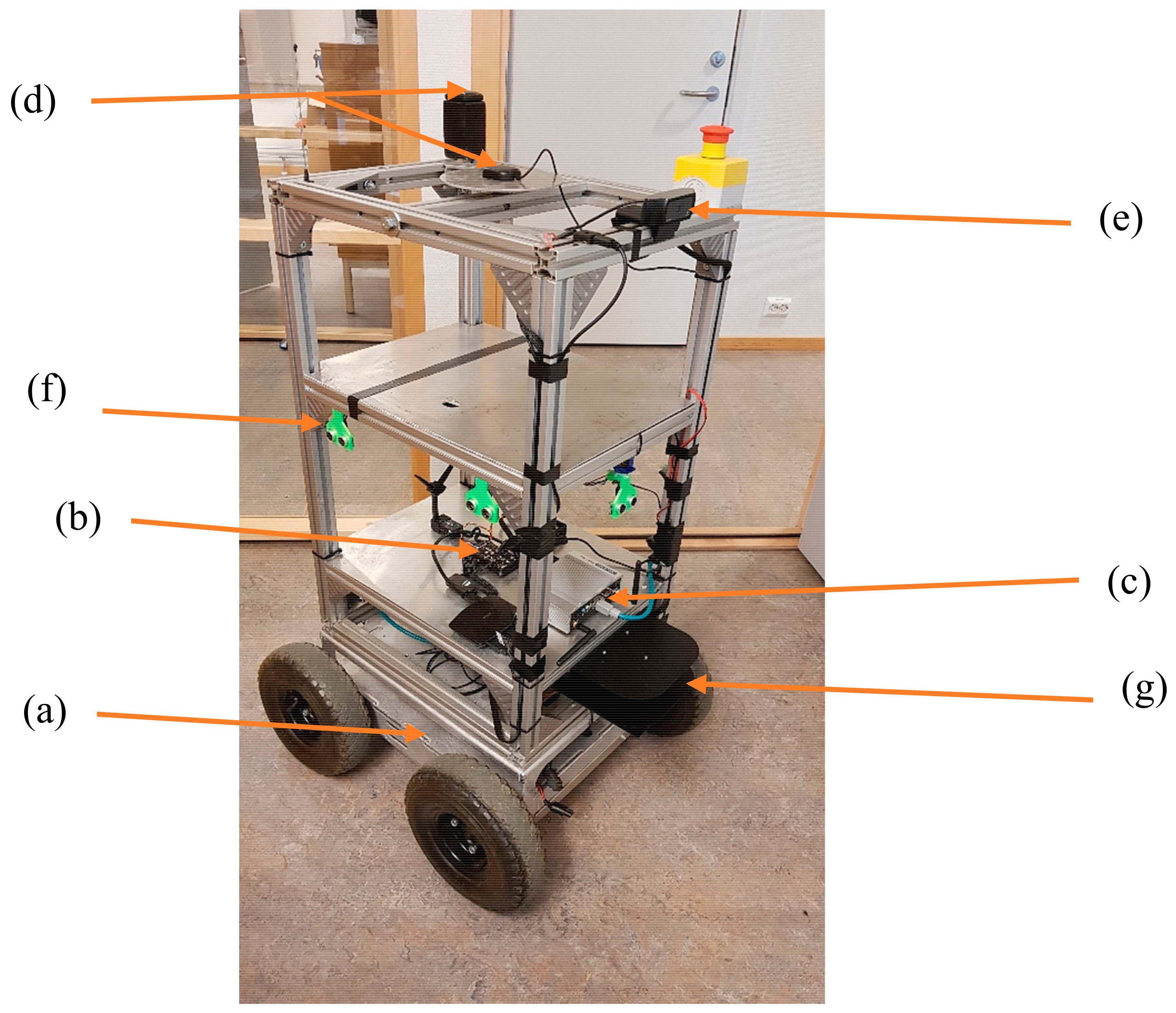
The mobile robot platform we selected as a starting point for this study is a combination of off-the-shelf components and structures developed at our center. The robot has an aluminum frame enabling sensors and actuators modularity, and its shape was designed for narrow places navigation (Figure 1).
The mobile carrying platform (IG52-DB4, Superdroid Robots, Fuquay-Varina, North Carolina, USA) is a 4 Wheels Drive platform (Figure 1a). It has four motors (one per wheel) with a maximum of 285 Rotations Per Minutes (RPM), and with 10 inches pneumatic wheels allowing a velocity up to 12 m/s. The steering mode for the platform is differential drive, where the linear and angular trajectories are obtained by changing the velocities of the motors (i.e., the rate of rotation of the wheels) on one side, relative to the velocities of the motors on the other side. The platform comes with two 12 V batteries, having a capacity of 18 Ah that allows for 2–5 h of operation time, depending on the payload and velocity. The motors drives are controlled using a pulse width modulation (PWM) signal coming from the autopilot board.
The autopilot board (Pixhaw Autopilot; Figure 1b) is the main bridge between the mobile carrying platform and the high level computer. It has a 168 MHz Cortex-M4F processor allowing 252 Million Instructions Per Seconds (MIPS). The board can be configured to control 14 PWM outputs, and it includes various communication interfaces: Inter-Integrated Circuit (I2C), Controller Area Network (CAN), and Universal Asynchronous Receiver/Transmitter (UART). The autopilot is linked to the high-level computer through a USB communication. The autopilot can be programmed independently of the high-level computer, using Mission Planner software (running on the base station). Manual control of the mobile robot is possible by means of a Taranis X9D remote controller, utilizing 2.4 GHz Radio Frequency (RF) communication.
The high level computer consists of an industrial grade embedded computer (ARK-1123H; Figure 1c). The computer has a quad core 2.0 GHz processor from Intel, coupled with 8 GB of RAM and 64 GB SSD storage. It is equipped with 2 Ethernet ports, 3 USB 2.0 inputs, 1 COM port (RS 232/422/485), and 1 HDMI output. Communication between the base station and the high-level computer is performed through WIFI communication, using a Secure Shell (SSH) network protocol.
For outdoor navigation, a GNSS receiver (uBlox, 3DR) was placed on top of the platform (Figure 1d). The GNSS has an update rate of 5 Hz, and the module also includes also a HMC5883L digital compass. For more accuracy, a Real Time Kinematic (RTK) GNSS receiver (Piksi, Swift Navigation) was added to the mobile robot. While the compass on the UBlox GNSS uses I2C bus, the GNSS receivers communicate with the low-level autopilot (Pixhawk board) through serial communication.
A RGB camera (C920, Logitech, Lausanne, Switzerland) was mounted on the upper front of the mobile robot (Figure 1e) for visual target tracking. The camera has a full HD 1080p resolution with an automatic low light correction and autofocus. The monocular camera was linked to the high-level computer through USB communication.
We equipped the mobile robot with six Ultra Sound (US) sensors (HC-SR04, Sparkfun, Boulder, CO, USA); two were mounted on each side, one on the front, and one on the back of the robot (Figure 1f). Since the sensors have analog output, we used an Arduino board (ARDUINO MEGA 2560, Arduino) for Analog to Digital Conversion (ADC). The Arduino board communicated with the high-level computer through USB communication.
A light detection and ranging (LIDAR) sensor (TiM 561, SICK, Waldkirch, Germany) was mounted on the lower front of the mobile robot (Figure 1g). The sensor has a planar aperture of 270° and a resolution of 0.33°. The scanning detection is up to 10 m at a frequency of 15 Hz. The LIDAR send the range readings through an Ethernet communication to the high-level computer.
An overview of the global architecture of the experimental platform as well as the communication type between each entity in the system is illustrated in Figure 2.
2.2. Software Architecture
In our setup, the high level computer is running a Linux distribution (Ubuntu 16.04). The robot operating system (ROS) [37] is the middleware that ensured communication between the different entities of the mobile robot through various nodes. An existing framework on ROS that allow the autonomous navigation of a mobile robot in an indoor environment is the move_base [38] framework. The main differences between the proposed scheme in this paper and this framework resides in that the latest requires odometry messages, AMCL (another framework to estimate the robots pose), the occupancy grid (a priori knowledge of the environment), and a map server in addition to the laser scans (or point clouds when using an RGBD or stereo vision camera). The work in this paper used the map only to define the navigation waypoints and for visualization purposes, while the laser scans are used for estimating the robot’s position (using the Hector SLAM), and extracting the obstacles’ locations. Thus, the simplicity of the present scheme is reflected in that the user needs to run two nodes in order to obtain the autonomous navigation scheme: the /hector_mapping node, and the /superdroid_nav node (/map_server on Figure 3 is used only for visualization purposes); more details on these two nodes will be explained further.
The communication between the low-level autopilot and the high-level computer was performed through the Mavros package, which is an adoption of Mavlink protocol used by the Pixhawk to ROS. The ROS Serial node allowed for the communication between the Arduino board and the high-level computer, in order to transmit the readings from the six US sensors. The LIDAR readings were obtained from the Sick_tim node, and the usb_cam node published the images gathered from the C920 camera (for visualization purposes in this work).
In addition to the localization and the autonomous navigation nodes, a launch file was created to start the aforementioned nodes. Figure 3 shows the active nodes running on the mobile robot during the execution of the autonomous navigation scheme that is explained in next section.
The /superdroid_nav node ran the autonomous navigation controller. This node subscribed to different topics:
- -
- /serial_node ran on the Arduino board. It published the readings obtained from the six US sensors mounted on the mobile robot.
- -
- /scan topic was the LIDAR readings published from /sick_tim551 node (the tim551 is compatible with the tim561 mounted of the mobile robot).
- -
- /hector_mapping subscribed to /scan topic and published the /slam_out_pose topic which is the relative pose (position and orientation) of the mobile robot.
The /superdroid_nav published the linear and angular velocities issued from the autonomous navigation controller to the following node:
- -
- /mavros/rc/override received velocity commands from /superdroid_nav, and emulated a generated signal from an RF controller, which was then turned by the Pixhawk board into PWM signals for the motors of the mobile carrying platform.
Other topics were not directly needed by the /superdroid_nav node, but their inclusion was for visualization purposes on Rviz:
- -
- /map_server published the map of the environment, which was used for the a priori selection of navigation waypoints, as well as for overlaying the current position of the mobile robot upon the prebuilt map.
- -
- /usb_cam published the images captured by the C920 camera mounted on the front of the mobile robot.
2.3. Simulation Software
The robot model and its environment were simulated on ROS using Gazebo and RViz. Figure 4 shows the 3D model of the mobile robot previously presented within the simulated greenhouse environment. The robots’ model was written using a unified robot description format (URDF), while Gazebo was used directly to simulate a greenhouse environment containing three rows of small plants and a wall surrounding them.
2.4. Experimental Environment
Experiments on the real platform were carried out in an office-like environment on the second floor of our research facility building, since the greenhouses had been dismantled for the winter when we performed this task. An office-like environment provides, however, a GNSS denied environment with row like structures (the corridors) not very unlike greenhouse conditions. Although the office-like environment did not provide any changes in the conditions due to plant growth, the frequency of human interference (colleagues passing by in the corridor) was higher than that expected in a greenhouse. All in all, we find that the test on the real platform was a valuable addition to the simulations, in order to validate our proposed approach.
3. Autonomous Navigation
Based on the work in [12], our mobile robot was designed to use a single LIDAR sensor in order to obtain the planar pose within a given environment (2D position and orientation). The used scheme was based on the comparison of the successive laser scans, where the resulting vector defined the movements of the platform. This technique is more robust compared to the conventional odometry, since it is not prone to slippage of the wheels. Nevertheless, since it is based on feature detection, a mismatch may result in an outlier localization when the surroundings has no features (moving inside a featureless corridor). However, we did not face such problems in our present study, since the navigation environment was rich with features, thus the probability of having outlier positioning was low as reflected in our experimental results (see Section 3.4).
To physically move the platform from its current position to its destination, we created a navigation scheme based on waypoints (i.e., a list of predefined locations was provided prior to the mission). The scheme allowed for a human operator to select waypoints on-the-go, as well as gaining back manual control of the mobile robot at any time, which is a necessary implementation to meet real world requirements.
We designed a control law that allowed the mobile robot to navigate through the given waypoints, while at the same time avoiding collision with static and dynamic obstacles. Our mobile robot was a non-holonomic platform (i.e., no lateral movements possible), and the kinematic model of the mobile robot is thus given by:
where and are the linear velocities in the mobile robots’ frame (Xr, Yr) respectively, while is its angular velocity. is the orientation of the mobile robot in the world frame (X, Y), while u and r are to be considered as the control inputs.
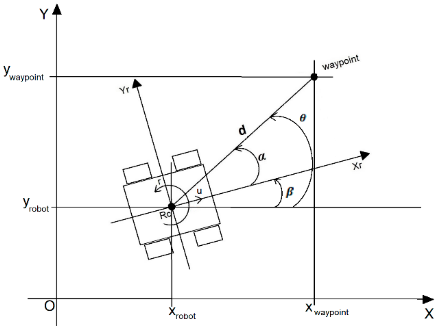
The coordinates of the waypoint were used in order to extract the distance d and angle α that separates the mobile robot from its goal (Figure 5), and generate the necessary linear u and angular r velocities. These entities are defined in the mobile robots’ frame (Xr, Yr), where Rc is the center of the platform.
Both the robots and the waypoints’ coordinates are represented in the world frame (X, Y). The robots’ coordinates were obtained from the ROS node /slam_out_pose previously explained, while the waypoints’ coordinates were extracted from the predefined list of desired trajectory, or by clicking on the desired location where the operator wants the mobile robot to reach.
The distance d is the Euclidian distance that separates the mobile robots’ position () from its destination (). It is expressed as:
The orientation α is given by:
where (the orientations of the mobile robot) is directly obtained from the /slam_out_pose node, and can be written as:
The results given by (atan) for a given angle are from the first and the fourth quadrant, regardless the origin of (tan) function. In our case we need to know in which quadrant the angle is located in order to send the correct information to the mobile robot, and this motivates the usage of the function (atan2) instead of (atan).
In order to move the mobile robot from its current position to its destination, the objective of the developed control law is to regulate the distance d and angle α as follows [39]:
The distance d and angle α are considered as the position and angular errors that separates the mobile robot to its platform. These errors need to be regulated in order to reach the given waypoint, however the control law will not depend only on them, but also on the obstacles that may come across the robot’s path. In the next section, our new controller for navigation and obstacle avoidance using artificial potential field (APF) application is presented.
3.1. Artificial Potential Field
Initially introduced for the control of robotic manipulators in [19], the application of APF for mobile robot’s navigation has been adapted, and since then widely used within the mobile robots research community. The main idea behind APF is to consider the mobile robot as a charged particle, while each point of the space is a field vector with a given intensity and direction. The initial position of the robot has the highest intensity with a vector pointing to the goal, which has the lowest one. In other words, the goal is considered as an attractive force that attracts the charged particle (the mobile robot) towards it, while static and dynamic obstacles within the environment are considered as repulsive forces that repulse the charged particle away from them.
The path of the mobile robot is defined by the force that results from the summation of the attractive and repulsive forces. We denote respectively and as the attractive and repulsive forces, while is the total force written by ( is the gradiant, and is the potential energy):
where:
The attractive force can be considered as the proportional term [19] related to the distance error between the robot and its waypoint, where is the positive attractive gain:
From (7) and (8), the expression of the attractive potential field can be written as follows:
The repulsive potential field of a given obstacle can be written as follows [40], where is the positive repulsive gain:
is the distance that separates the mobile robot from its obstacles. This distance is taken into consideration only when the obstacle is detected within a threshold , otherwise the obstacle is ignored, and is considered infinite:
The application of APF allows the mobile robot to avoid existing obstacles present in its path by contouring them. In constrained environments, such as greenhouses, contouring an obstacle present on the trajectory of the robot is a challenging task, because the rows are narrow, and no room is available for safe obstacle contouring. The map of the environment is predefined, thus the trajectory of the robots (the given waypoints) are supposed to be obstacle free (the static ones). This implies that the only possible obstacle is a moving one, which most likely would be a human worker. If such an obstacle approaches the area in front of the robot, the robot enters into a passive motion safety [41], which means that the robot simply stops then steps back a few centimeters and waits until the human passes to resume its trajectory. Thus, an assumption is that the repulsive potential field taken into consideration is the one present on the sides of the robots, where it will be used to keep a safe distance when moving in a constrained environment, allowing the robot to adapt to the dynamic changes inside the greenhouse due to the crops growth.
Based on the aforementioned assumption, the linear motion of the robot is directly related to the distance between the robot and its waypoints (the attractive force). The rotational motion is related to the angle between the mobile robot and its waypoint, and additionally to the repulsive force presents on the sides of the robot. Hence, the controller for steering the mobile robot towards its goal including the attractive and repulsive forces is written as follows, where is the positive angular gain:
From (12), we can see that both a long distance and a big angle induce high values of and , which results in high linear and angular velocities that lead to undesirable behavior of the physical robot and may damage its actuators. We have therefore included a saturation to limit the speed to an allowable upper bound for linear velocities (dmax). The linear velocity may thus be expressed as:
As for the angular velocities, similar approach has been followed when dealing with big angles (when , ):
The values of , ,, and are to be defined experimentally.
3.2. Simulation Results
To visualize the readings from the robots’ sensors (LIDAR), and to display its pose (2D position and orientation) within the environment, we used RViz on ROS (Figure 6).
The mapping of the environment has been performed prior to the waypoints mission. The enumerated dots on Figure 6 indicate the predefined waypoints for the robots’ navigation, and the direction of movement was from the lower number to the higher one. Once the mobile robot reached waypoint number 7, it navigated back to its starting point (waypoint 0).
The variation in distance d and angle α over time are illustrated in Figure 7 and Figure 8, respectively. The peaks on both graphs represent the moment when the robot initiated a new waypoint, which means that a new distance d and angle α were introduced to the controller. The robot was considered to have reached its waypoint when it was located when ( = 30) Equation (13). This effectively prevented the robot from roaming around a waypoint, mainly in cases when the robot couldn’t perfectly align its orientation to its target. The distance that separated the robot and its waypoint decreased over time (Figure 7). Similarly, the angle α also decreased over time (Figure 8). The small variations in angles observed between the major shifts (Figure 8) are due to the leaves that are considered as repulsive forces. The trajectory of the robot within the simulated greenhouse can be seen in Figure 9.
The simulation results showed that the proposed controller was efficient Equation (12), and that the control objective Equation (5) has been satisfied.
3.3. Dynamic Plant Development Simulation
In order to simulate the navigation scheme taking in consideration plan developments, a new simulated greenhouse with different trees position has been simulated. The waypoints list as well as the initial position of the mobile robot are the same as previously described.
Figure 10 shows the grid map of the new simulated environment.
The trajectory of the robot can be seen in Figure 11, while Figure 12 gives an overview of the robots’ pose within the greenhouse rows in the 3D simulated model.
Even though the passage between the rows was narrow (Figure 12), the controller developed allowed the robot to navigate safely between the trees, which confirms the efficiency of the proposed controller.
3.4. Experimental Results
As in the simulation, a first step consisted in mapping the environment using the /hector_mapping node previously presented. The processed map was then used to define the navigation waypoints within the environment (Figure 13).
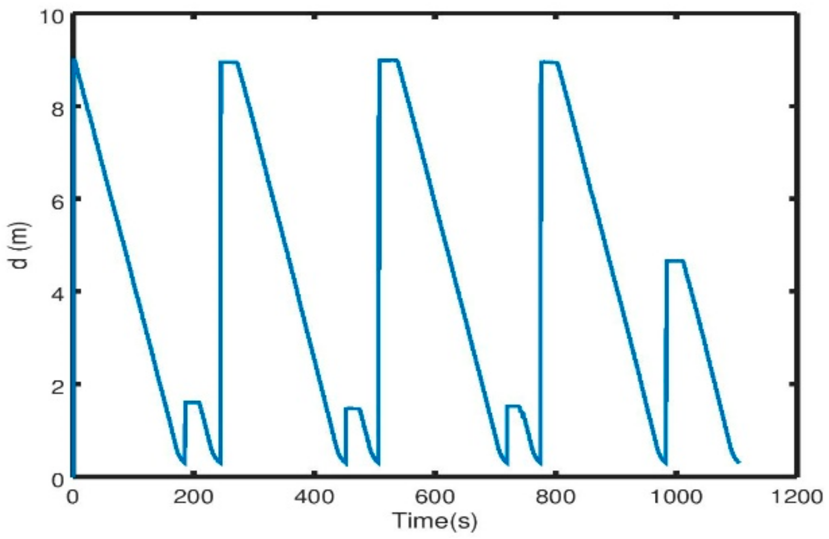
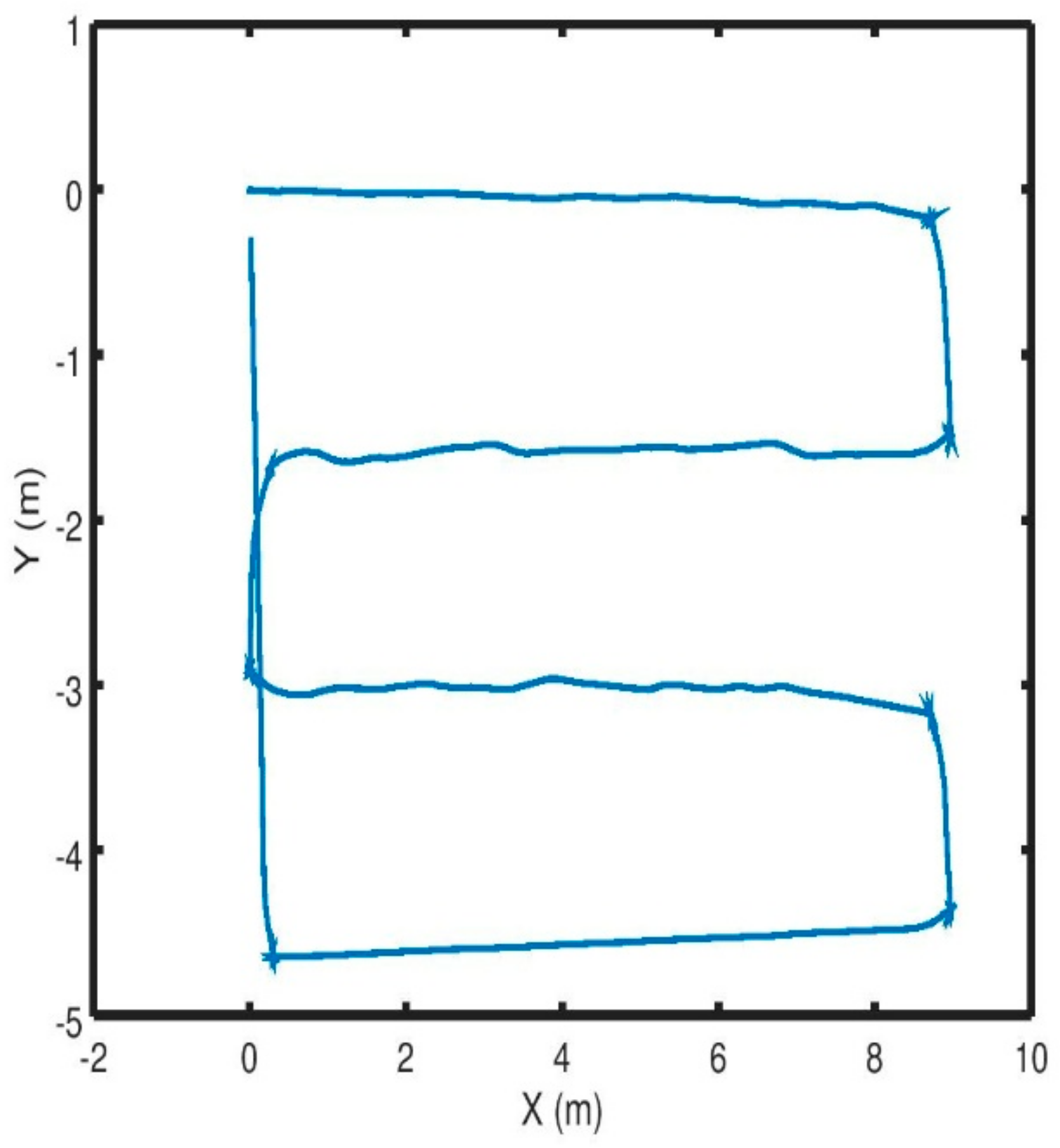
Waypoint navigation was performed so that the robot moved between the waypoints in the following order: 0 => 1 => 2 => 3 => 2 => 0. The variation over time of both d (Figure 14) and α (Figure 15) was observed in order to evaluate the performance of the proposed controller on the real platform. The trajectory of the robot is shown in Figure 16.
The waypoints distribution implied that at waypoint 1 and 3 the robot needed to turn 180°. In tight environments as the corridors (or between plant rows in a greenhouse), the robot is facing the wall after turning 90°, and the front obstacle detection is thereby triggered. As we previously stated, the robot enters in an idle state (or actually steps back a few centimeters) waiting for the supposed obstacle (human) to be collaborative and free the path. This slight step back movement allows the robot to keep turning slowly until the front is headed towards a free space again, where the robot resumes its normal trajectory. This can be clearly seen in Figure 14, where upon the reception of the second waypoint, the robot finds itself facing a 180° turn, which explains that the distance between the robot and its next waypoint is almost constant while the angle α as we can see in Figure 15 is decreasing. The same thing happens when the robot arrives to waypoint 3 and turns to waypoint 4.
The experimental results confirmed the findings from the simulations. The proposed controller appeared to work efficiently on the real platform, and the tests showed that the condition Equation (5) of the proposed controller Equation (12) has been met.
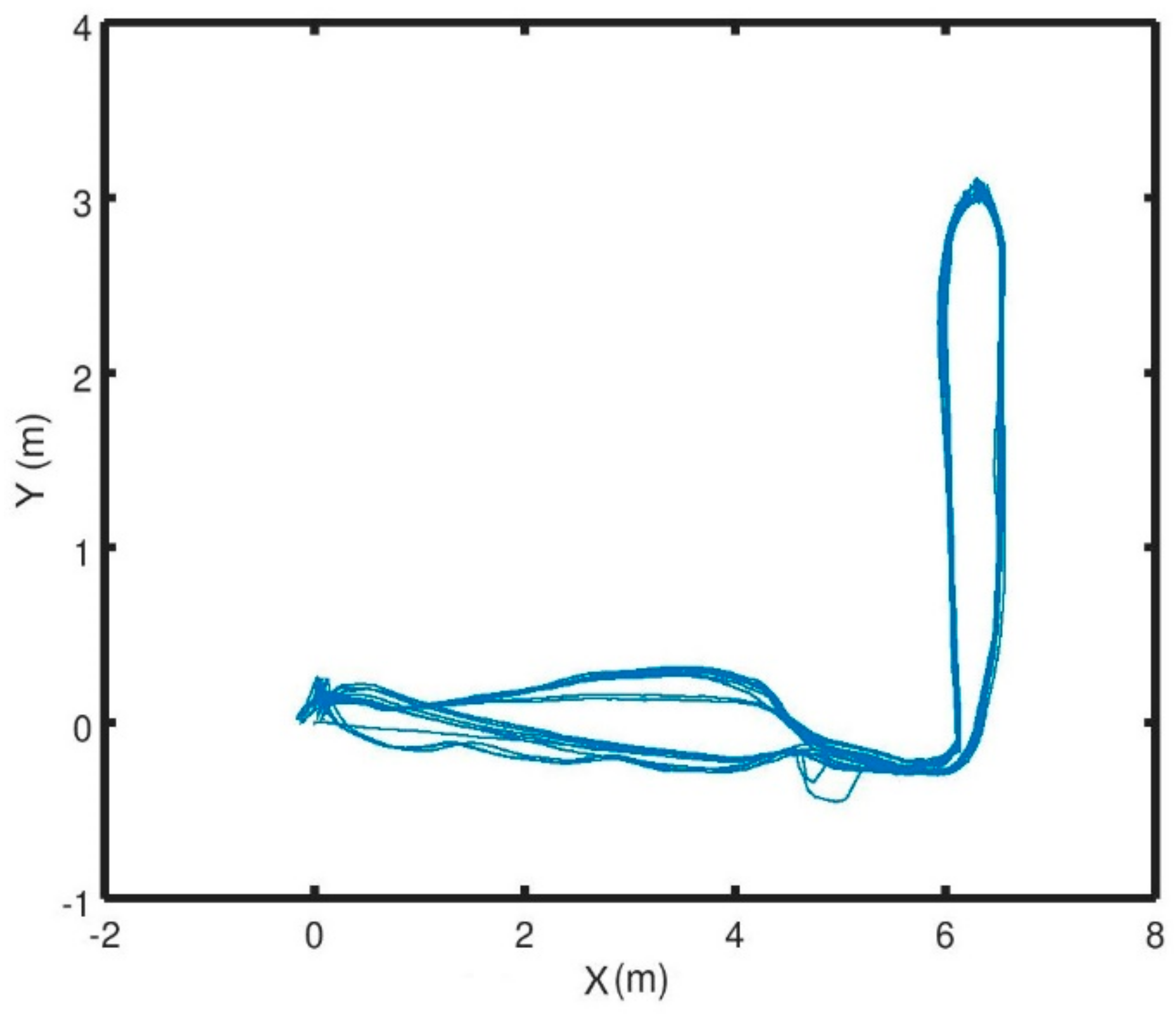
3.5. Robustness: Experimental Analysis
In order to check the robustness of the proposed scheme experimentally, we performed the same experimental setup with waypoints (0 => 2 => 3 => 4 => 0) repeatedly (see Figure 13 for waypoints positions). This meant that each time the robot had driven through one cycle, it started again without any intervention to recalibrate its position. We performed 10 cycles, and the trajectory of the robot can be seen in Figure 17.
The repetitive experimenting was conducted during working hours. This implied that some colleagues passed close to the robot during driving, and some of them even “teased it” by standing on its way to check its reaction. This explains some of the deviation from one trajectory to another. However, this also confirms the robustness of the proposed scheme to real conditions and to repeatability.
4. Conclusions
In this paper we presented a novel solution for indoor navigation of a mobile robot (i.e., in a GNSS-denied environment typical for a greenhouse). The robot can freely move inside the greenhouse without any physical guidance system mounted on the ground. The localization of the robot was obtained using a single LIDAR sensor mounted on the front of the robot using the open source Hector SLAM for pose estimation, and the autonomous navigation is ensured thanks to the APF controller developed. We showed that the robot is able to adapt to the structural changes due to the growth of the crops while being safe to operate in the presence of humans. We illustrated in this paper the hardware and software setup of the mobile robot. The proposed scheme was validated through simulation and real experiments, showing promising results, especially for repeatability without external rectifiers. Future work will comprise testing the proposed controller more thoroughly in a greenhouse, including experiments performed over longer periods.
Author Contributions
El Houssein Chouaib Harik conceived, designed and performed the experiments, analyzed the data, and wrote with Audun Korsæth the paper.
Funding
The development of the robots’ hardware as well as the navigation scheme presented in this paper is funded by the Center for Precision Agriculture at the Norwegian Institute of Bioeconomy (NIBIO) in Norway.
Acknowledgments
The authors would like to thank Maximilian Pircher for his help in the hardware development of the presented platform.
Conflicts of Interest
The authors declare no conflict of interest.
References
- Vakilian, K.A.; Massah, J. A farmer-assistant robot for nitrogen fertilizing management of greenhouse crops. Comput. Electron. Agric. 2017, 139, 153–163. [Google Scholar] [CrossRef]
- Durmuş, E.O.G.; Kırcı, M. Data acquisition from greenhouses by using autonomous mobile robot. In Proceedings of the 2016 Fifth International Conference on Agro-Geoinformatics (Agro-Geoinformatics), Tianjin, China, 18–20 July 2016. [Google Scholar]
- Schor, N.; Bechar, A.; Ignat, T.; Dombrovsky, A.; Elad, Y.; Berman, S. Robotic disease detection in greenhouses: Combined detection of powdery mildew and tomato spotted wilt virus. IEEE Robot. Autom. Lett. 2016, 1, 354–360. [Google Scholar] [CrossRef]
- Van Henten, E.J.; Hemming, J.; Van Tuijl, B.A.J.; Kornet, J.G.; Meuleman, J.; Bontsema, J.; Van Os, E.A. An autonomous robot for harvesting cucumbers in greenhouses. Auton. Robot. 2002, 13, 241–258. [Google Scholar] [CrossRef]
- Gat, G.; Gan-Mor, S.; Degani, A. Stable and robust vehicle steering control using an overhead guide in greenhouse tasks. Comput. Electron. Agric. 2016, 121, 234–244. [Google Scholar] [CrossRef]
- Grimstad, L.; From, P.J. The Thorvald II Agricultural Robotic System. Robotics 2017, 6, 24. [Google Scholar] [CrossRef]
- Nakao, N.; Suzuki, H.; Kitajima, T.; Kuwahara, A.; Yasuno, T. Path Planning and Traveling Control for Pesticide-Spraying Robot in Greenhouse. J. Signal Process. 2017, 21, 175–178. [Google Scholar] [CrossRef]
- González, R.; Rodríguez, F.; Sánchez-Hermosilla, J.; Donaire, J.G. Navigation techniques for mobile robots in greenhouses. Appl. Eng. Agric. 2009, 25, 153–165. [Google Scholar] [CrossRef]
- Thrun, S. Robotic mapping: A survey. In Exploring Artificial Intelligence in the New Millennium; Morgan Kaufmann: Burlington, MA, USA, 2002; Volume 1, pp. 1–35. [Google Scholar]
- Xue, J.; Fan, B.; Zhang, X.; Feng, Y. An Agricultural Robot for Multipurpose Operations in a Greenhouse. DEStech Trans. Eng. Technol. Res. 2017. [Google Scholar] [CrossRef]
- Reiser, D.; Miguel, G.; Arellano, M.V.; Griepentrog, H.W.; Paraforos, D.S. Crop row detection in maize for developing navigation algorithms under changing plant growth stages. In Robot 2015: Second Iberian Robotics Conference; Springer: Cham, Switzerland, 2016. [Google Scholar]
- Kohlbrecher, S.; Meyer, J.; Graber, T.; Petersen, K.; Klingauf, U.; Stryk, O. Hector open source modules for autonomous mapping and navigation with rescue robots. In Proceedings of the Robot Soccer World Cup, Eindhoven, The Netherlands, 24–30 June 2013. [Google Scholar]
- Kohlbrecher, S.; Meyer, J.; Graber, T.; Petersen, K.; Von Stryk, O.; Klingauf, U. Robocuprescue 2014-robot league team hector Darmstadt. In Proceedings of the RoboCupRescue 2014, João Pessoa, Brazil, 20–24 July 2014. [Google Scholar]
- Hoy, M.; Matveev, A.S.; Savkin, A.V. Algorithms for collision-free navigation of mobile robots in complex cluttered environments: A survey. Robotica 2015, 33, 463–497. [Google Scholar] [CrossRef]
- Valbuena, L.; Tanner, H.G. Hybrid potential field based control of differential drive mobile robots. J. Intell. Robot. Syst. 2012, 68, 307–322. [Google Scholar] [CrossRef]
- Zhu, Y.; Özgüner, Ü. Constrained model predictive control for nonholonomic vehicle regulation problem. IFAC Proc. Vol. 2008, 41, 9552–9557. [Google Scholar] [CrossRef]
- Yang, K.; Moon, S.; Yoo, S.; Kang, J.; Doh, N.L.; Kim, H.B.; Joo, S. Spline-based RRT path planner for non-holonomic robots. J. Intell. Robot. Syst. 2014, 73, 763–782. [Google Scholar] [CrossRef]
- Arismendi, C.; Álvarez, D.; Garrido, S.; Moreno, L. Nonholonomic motion planning using the fast marching square method. Int. J. Adv. Robot. Syst. 2015, 12, 56. [Google Scholar] [CrossRef]
- Khatib, O. Real-time obstacle avoidance for manipulators and mobile robots. Int. J. Robot. Res. 1986, 5, 90–98. [Google Scholar] [CrossRef]
- Iswanto, I.; Wahyunggoro, O.; Cahyadi, A.I. Path Planning Based on Fuzzy Decision Trees and Potential Field. Int. J. Electr. Comput. Eng. 2016, 6, 212. [Google Scholar] [CrossRef]
- Sgorbissa, A.; Zaccaria, R. Planning and obstacle avoidance in mobile robotics. Robot. Auton. Syst. 2012, 60, 628–638. [Google Scholar] [CrossRef]
- Masoud, A.A.; Ahmed, M.; Al-Shaikhi, A. Servo-level, sensor-based navigation using harmonic potential fields. In Proceedings of the 2015 European Control Conference (ECC), Linz, Austria, 15–17 July 2015. [Google Scholar]
- Rodrigues, R.T.; Basiri, M.; Aguiar, A.P.; Miraldo, P. Low-level Active Visual Navigation Increasing robustness of vision-based localization using potential fields. IEEE Robot. Autom. Lett. 2018, 3, 2079–2086. [Google Scholar] [CrossRef]
- Rodrigues, R.T.; Basiri, M.; Aguiar, A.P.; Miraldo, P. Feature Based Potential Field for Low-level Active Visual Navigation. In Proceedings of the Iberian Robotics Conference, Sevilla, Spain, 22–24 November 2017. [Google Scholar]
- Mur-artal, R.; Montiel, J.M.M.; Tardos, J.D. ORB-SLAM: A versatile and accurate monocular SLAM system. IEEE Trans. Robot. 2015, 31, 1147–1163. [Google Scholar] [CrossRef]
- Li, W.; Yang, C.; Jiang, Y.; Liu, X.; Su, C.-Y. Motion planning for omnidirectional wheeled mobile robot by potential field method. J. Adv. Transp. 2017, 2017, 4961383. [Google Scholar] [CrossRef]
- Lee, M.C.; Park, M.G. Artificial potential field based path planning for mobile robots using a virtual obstacle concept. In Proceedings of the 2003 IEEE/ASME International Conference on Advanced Intelligent Mechatronics (AIM 2003), Kobe, Japan, 20–24 July 2003. [Google Scholar]
- Kuo, P.-L.; Wang, C.-H.; Chou, H.-J.; Liu, J.-S. A real-time streamline-based obstacle avoidance system for curvature-constrained nonholonomic mobile robots. In Proceedings of the 2017 6th International Symposium on Advanced Control of Industrial Processes (AdCONIP), Taipei, Taiwan, 28–31 May 2017. [Google Scholar]
- Urakubo, T. Stability analysis and control of nonholonomic systems with potential fields. J. Intell. Robot. Syst. 2018, 89, 121–137. [Google Scholar] [CrossRef]
- Poonawala, H.A.; Satici, A.C.; Eckert, H.; Spong, M.W. Collision-free formation control with decentralized connectivity preservation for nonholonomic-wheeled mobile robots. IEEE Trans. Control Netw. Syst. 2015, 2, 122–130. [Google Scholar] [CrossRef]
- Shimoda, S.; Kuroda, Y.; Iagnemma, K. Potential field navigation of high speed unmanned ground vehicles on uneven terrain. In Proceedings of the 2005 IEEE International Conference on Robotics and Automation (ICRA 2005), Barcelona, Spain, 18–22 April 2005. [Google Scholar]
- Zhu, Q.; Yan, Y.; Xing, Z. Robot path planning based on artificial potential field approach with simulated annealing. In Proceedings of the Sixth International Conference on Intelligent Systems Design and Applications (ISDA’06), Jinan, China, 16–18 October 2006. [Google Scholar]
- Yun, X.; Tan, K.-C. A wall-following method for escaping local minima in potential field based motion planning. In Proceedings of the 8th International Conference on Advanced Robotics (ICAR’97), Monterey, CA, USA, 7–9 July 1997. [Google Scholar]
- Guerra, M.; Efimov, D.; Zheng, G.; Perruquetti, W. Avoiding local minima in the potential field method using input-to-state stability. Control Eng. Pract. 2016, 55, 174–184. [Google Scholar] [CrossRef]
- Warren, C.W. Global path planning using artificial potential fields. In Proceedings of the 1989 IEEE International Conference on Robotics and Automation, Scottsdale, AZ, USA, 14–19 May 1989. [Google Scholar]
- Siegwart, R.; Nourbakhsh, I.R.; Scaramuzza, D. Introduction to Autonomous Mobile Robots; MIT Press: Cambridge, MA, USA, 2011. [Google Scholar]
- Quigley, M.; Conley, K.; Gerkey, B.; Faust, J.; Foote, T.; Leibs, J.; Wheeler, R.; Ng, A.Y. ROS: An open-source Robot Operating System. In Proceedings of the ICRA Workshop on Open Source Software, Kobe, Japan, 12–17 May 2009. [Google Scholar]
- Move_base Package. Available online: http://wiki.ros.org/move_base (accessed on 16 April 2018).
- Harik, E.H.C.; Guerin, F.; Guinand, F.; Brethe, J.-F.; Pelvillain, H. A decentralized interactive architecture for aerial and ground mobile robots cooperation. In Proceedings of the IEEE International Conference on Control, Automation and Robotics (ICCAR 2015), Singapore, 20–22 May 2015. [Google Scholar]
- Triharminto, H.H.; Wahyunggoro, O.; Adji, T.B.; Cahyadi, A.I. An Integrated Artificial Potential Field Path Planning with Kinematic Control for Nonholonomic Mobile Robot. Int. J. Adv. Sci. Eng. Inf. Technol. 2016, 6, 410–418. [Google Scholar] [CrossRef]
- Bouraine, S.; Fraichard, T.; Salhi, H. Provably safe navigation for mobile robots with limited field-of-views in dynamic environments. Auton. Robot. 2012, 32, 267–283. [Google Scholar] [CrossRef]
Figure 1.
The mobile robot consisting of: (a) a mobile platform (IG52-DB4 Superdroidrobots), (b) an autopilot (Pixhaw), (c) an embedded computer (ARK-1123H), (d) a GNSS-receiver (uBlox, 3DR), (e) a camera (C920, Logitech), (f) an ultrasound sensor (HC-SR04), and (g) a light detection and ranging (LIDAR) sensor (TiM 561, SICK).

Figure 2.
Hardware architecture of the mobile robot.
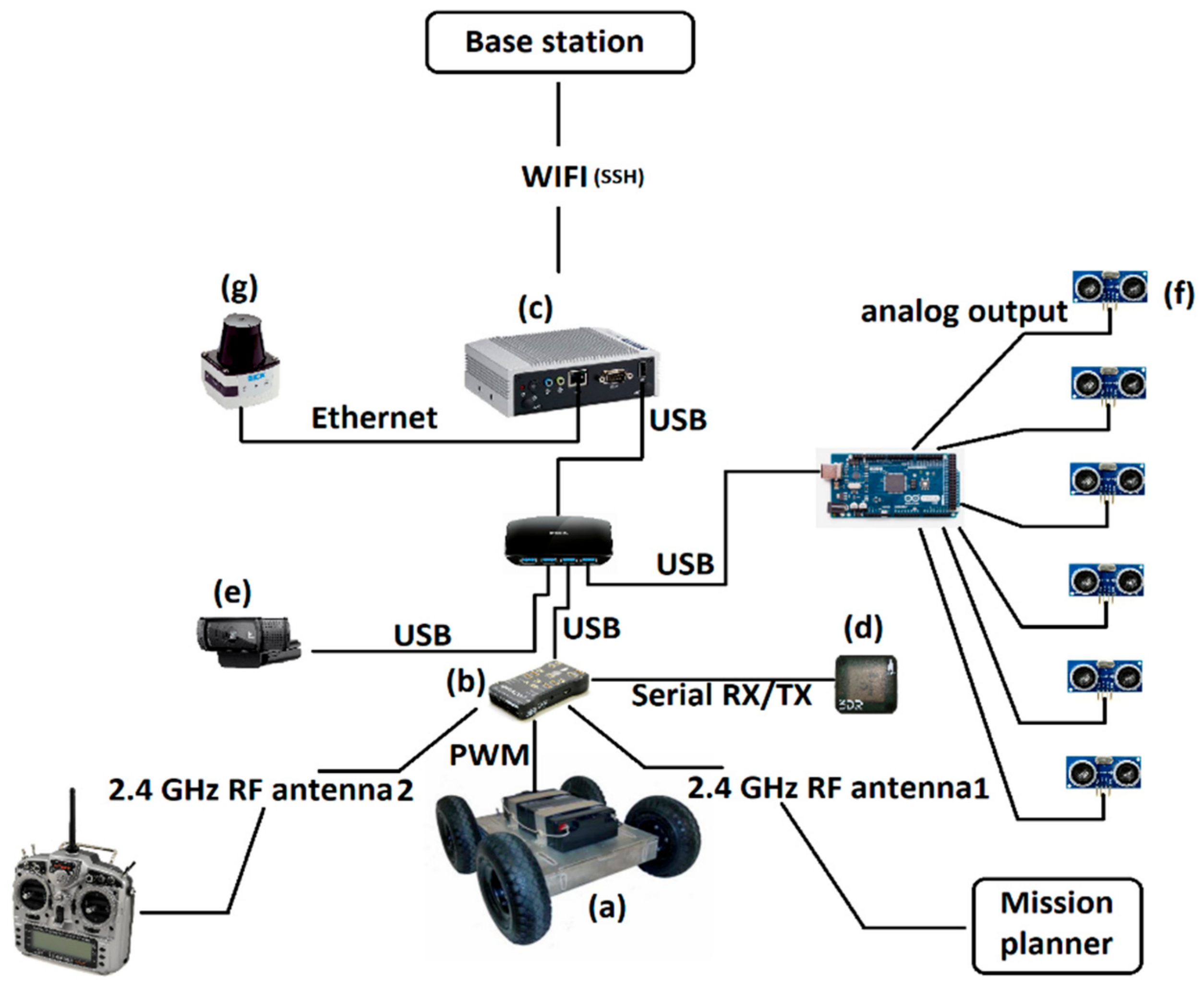
Figure 3.
Software architecture: running nodes on the robot operating system (ROS).
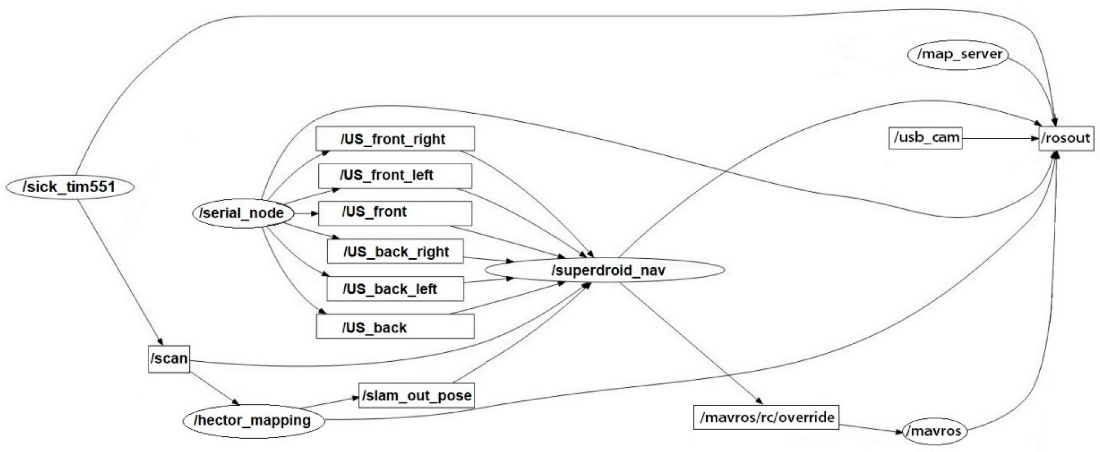
Figure 4.
The simulated models of the mobile robot and the greenhouse.
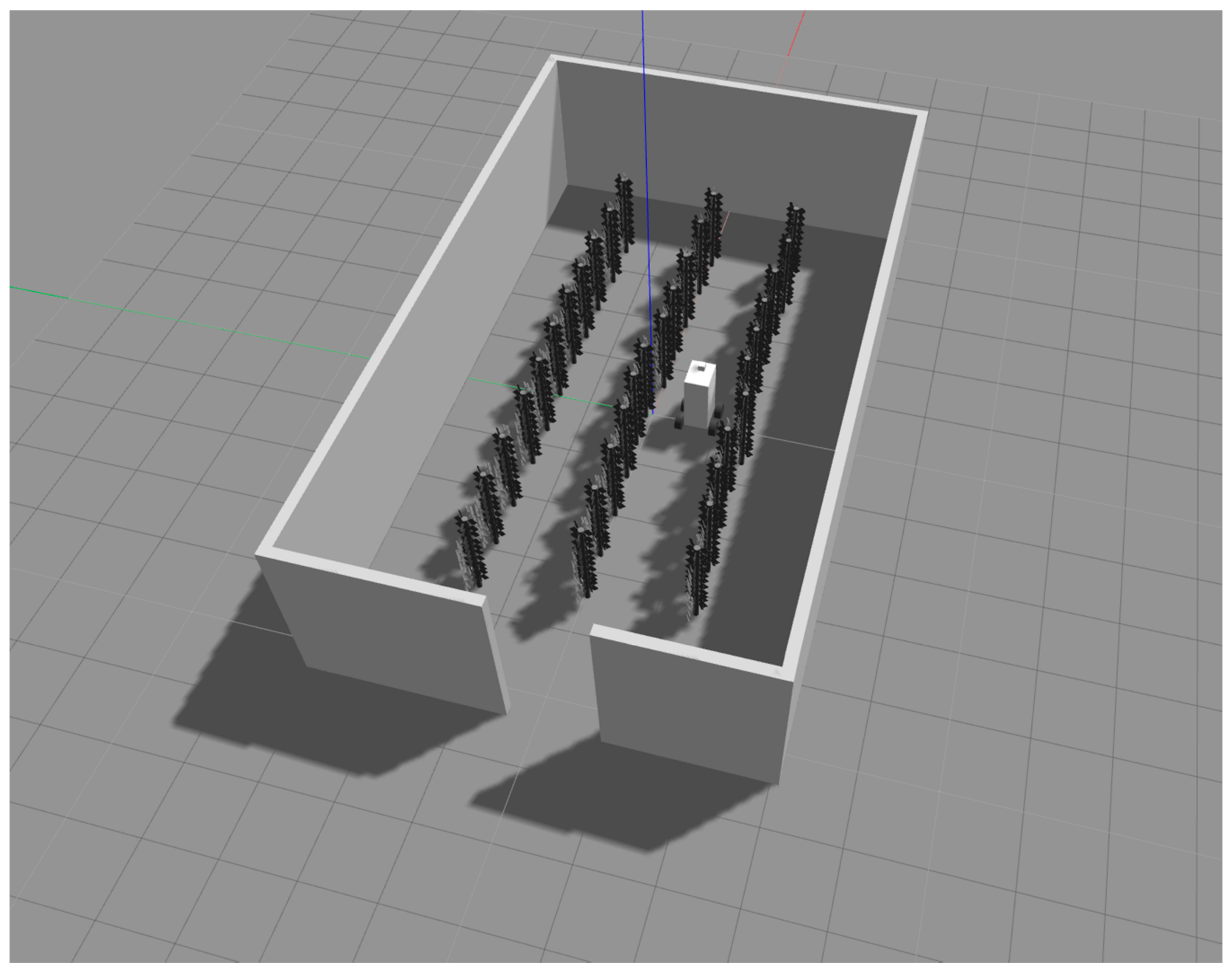
Figure 5.
Design of the mobile robots’ control law.

Figure 6.
Robots’ state visualization on RViz from the greenhouse simulated environment. Waypoints are represented by red dots, and enumerated by their passage order. Free space is represented by white color, known obstacles are represented by black color, and unknown space is represented by grey color.
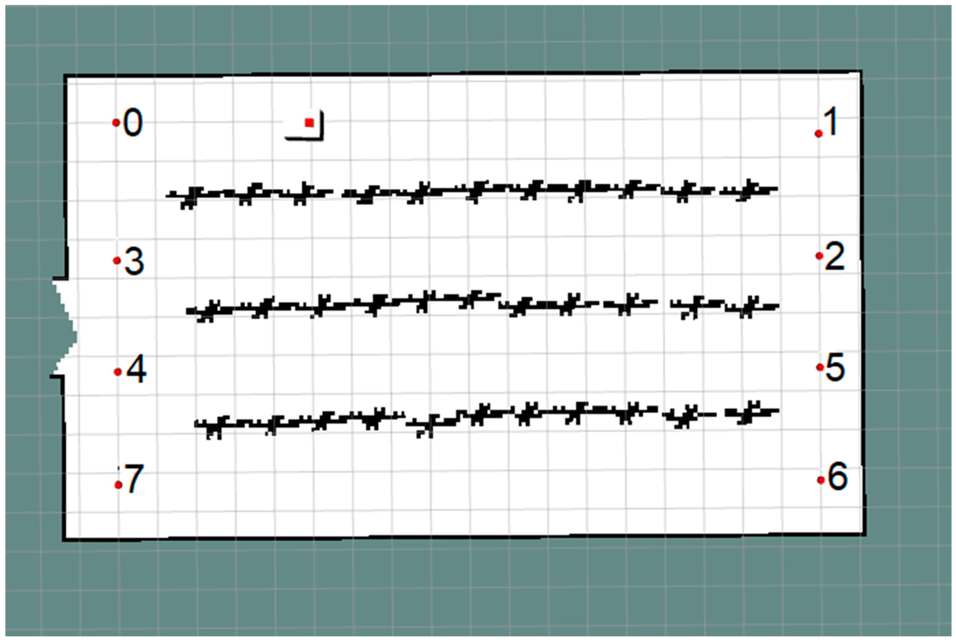
Figure 7.
Distance variation between the robot and the next waypoint in simulation.

Figure 8.
Angle variation between the robot and the next waypoint in simulation.
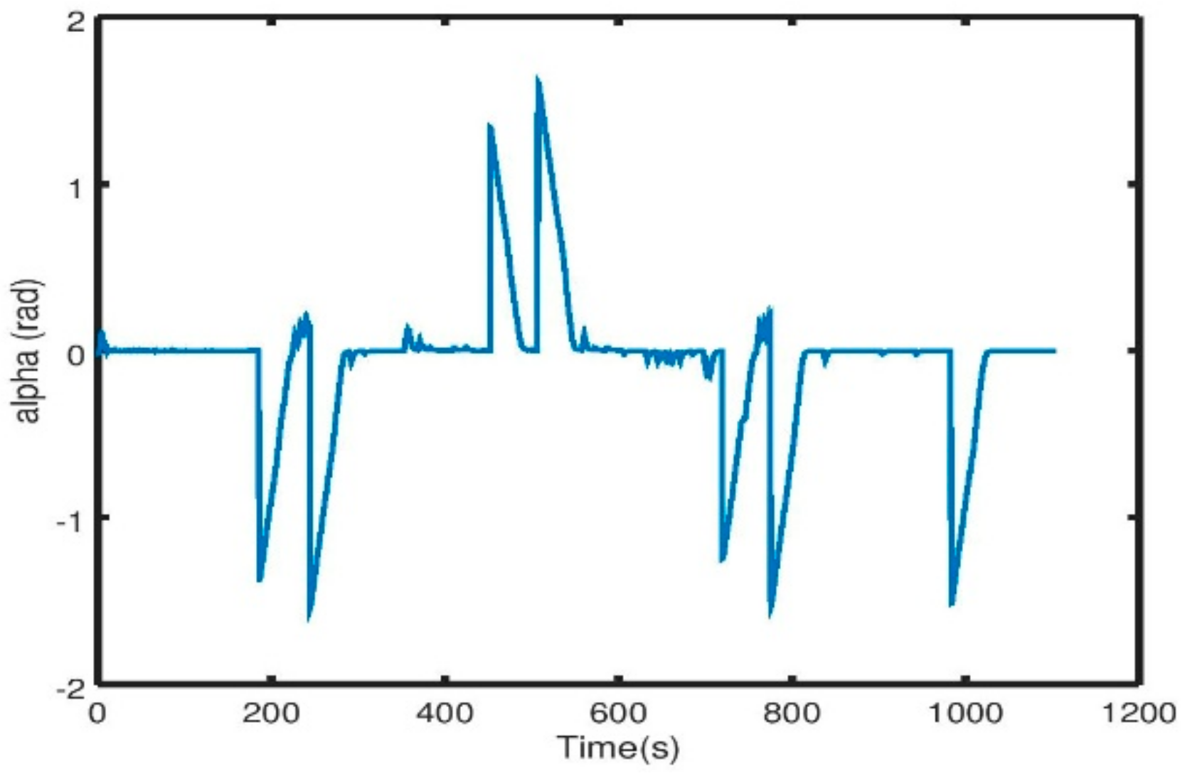
Figure 9.
The trajectory of the robot in simulation.
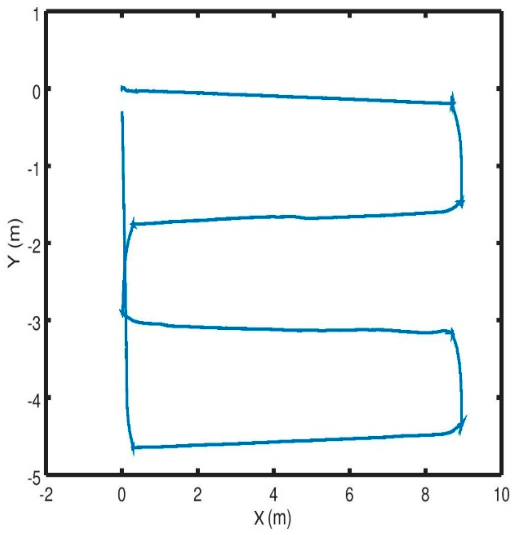
Figure 10.
The grid map of the new simulated environment.
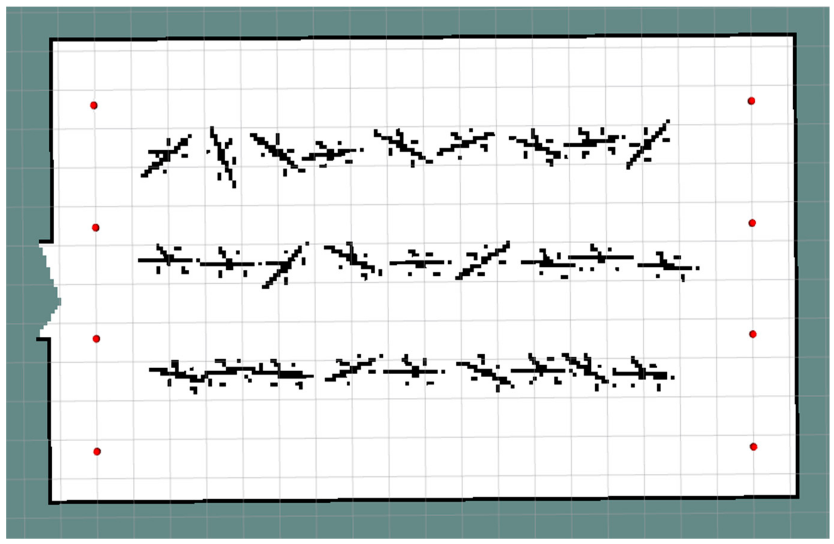
Figure 11.
The trajectory of the robot in simulation.

Figure 12.
The robots’ pose within the new simulated environment.
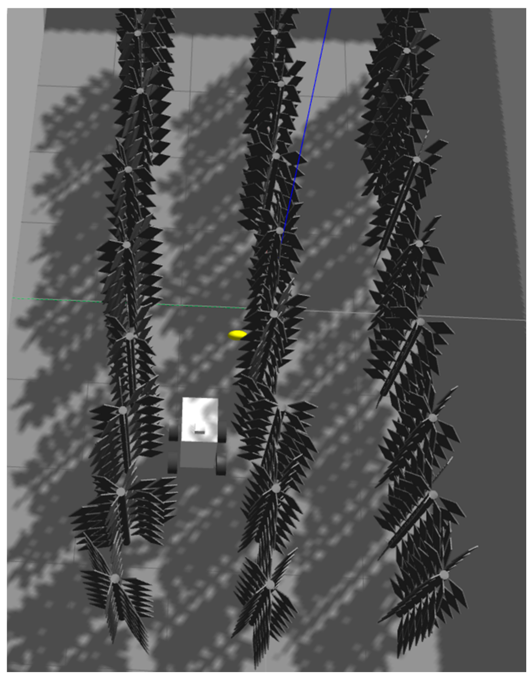
Figure 13.
Indoor waypoints navigation. Waypoints are represented by red dots, and enumerated by their passage order. Free space is represented by white color, known obstacles are represented by black color, and unknown space is represented by grey color.
Figure 13.
Indoor waypoints navigation. Waypoints are represented by red dots, and enumerated by their passage order. Free space is represented by white color, known obstacles are represented by black color, and unknown space is represented by grey color.
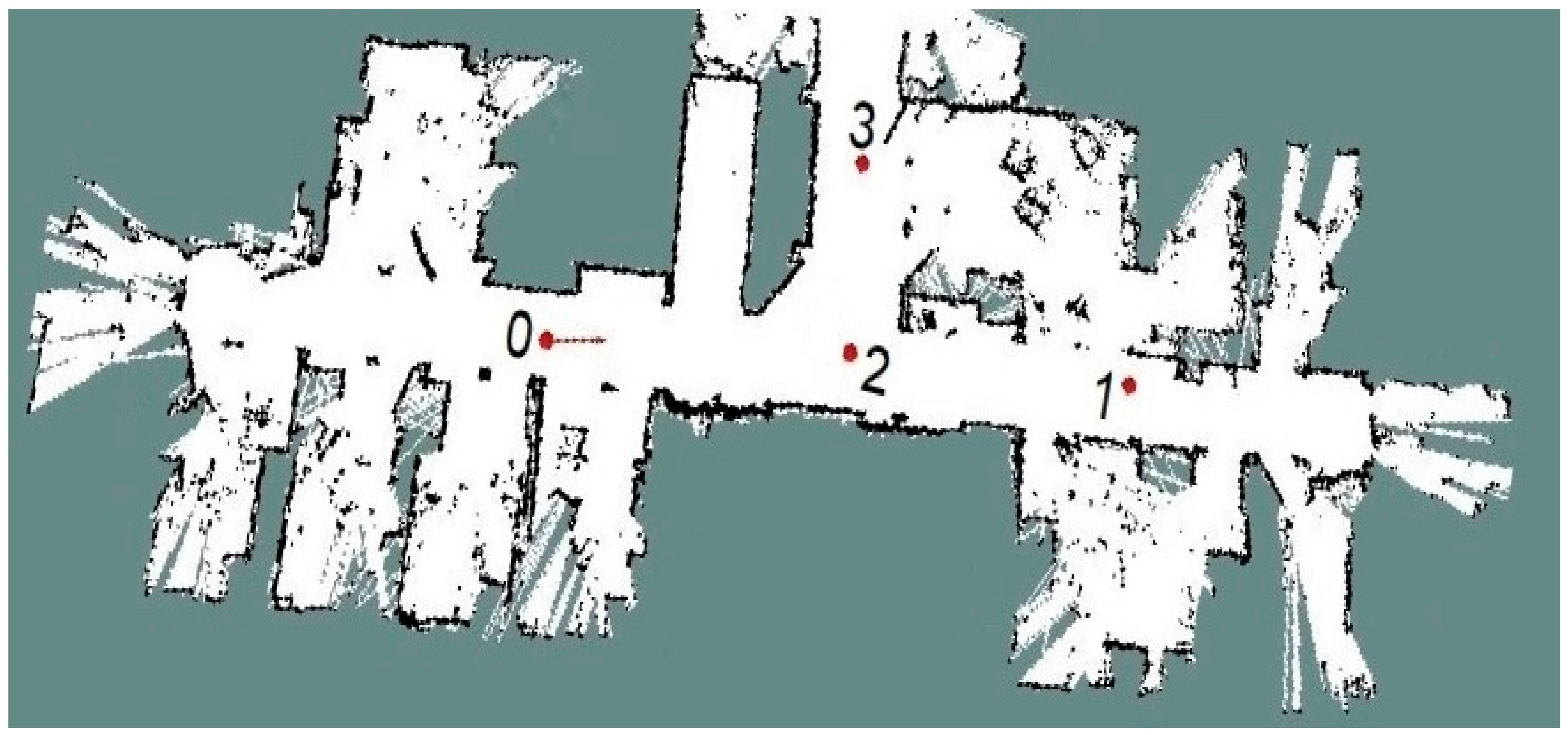
Figure 14.
Distance variation between the robot and the next waypoint in experiments.
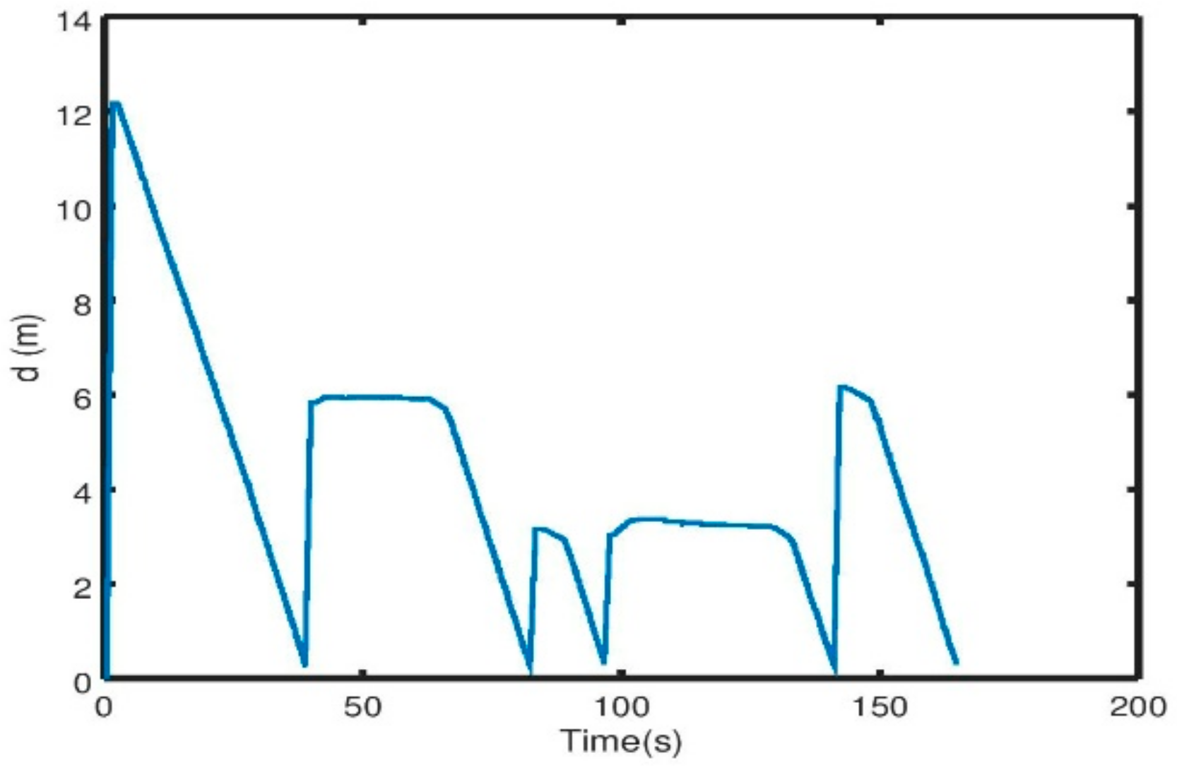
Figure 15.
Angle variation between the robot and the next waypoint in experiments.
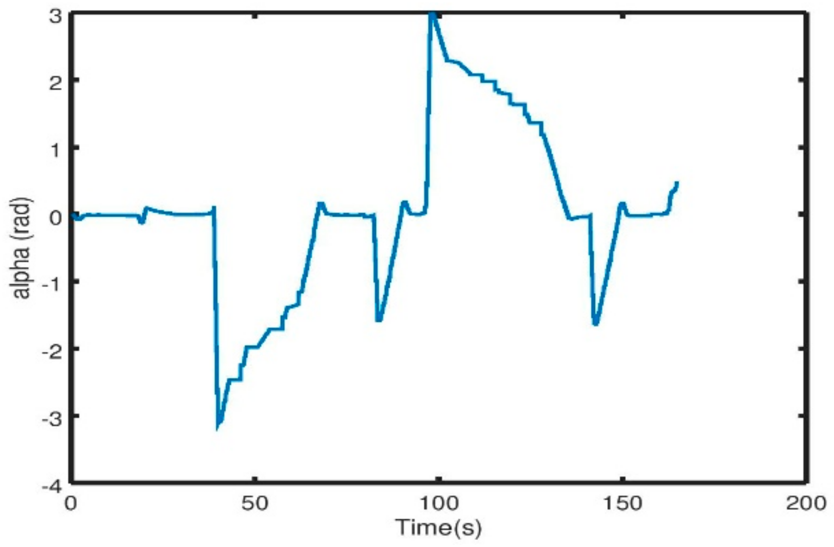
Figure 16.
The trajectory of the robot in experiments.
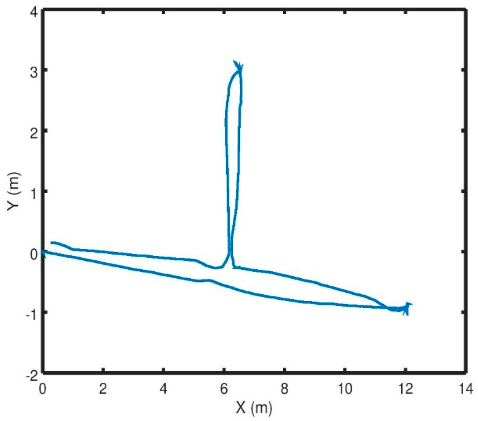
Figure 17.
Repetitive trajectory.

© 2018 by the authors. Licensee MDPI, Basel, Switzerland. This article is an open access article distributed under the terms and conditions of the Creative Commons Attribution (CC BY) license (http://creativecommons.org/licenses/by/4.0/).
Share and Cite
MDPI and ACS Style
Harik, E.H.C.; Korsaeth, A. Combining Hector SLAM and Artificial Potential Field for Autonomous Navigation Inside a Greenhouse. Robotics 2018, 7, 22. https://doi.org/10.3390/robotics7020022
AMA Style
Harik EHC, Korsaeth A. Combining Hector SLAM and Artificial Potential Field for Autonomous Navigation Inside a Greenhouse. Robotics. 2018; 7(2):22. https://doi.org/10.3390/robotics7020022
Chicago/Turabian StyleHarik, El Houssein Chouaib, and Audun Korsaeth. 2018. "Combining Hector SLAM and Artificial Potential Field for Autonomous Navigation Inside a Greenhouse" Robotics 7, no. 2: 22. https://doi.org/10.3390/robotics7020022
Note that from the first issue of 2016, this journal uses article numbers instead of page numbers. See further details here.