1. Introduction
Robot technology is focused on increasing the quality of life by the creation of new machines and methods. This paper reports on the development of a snow-removal robot called
SnowEater. The concept for this robot is the creation of a safe, slow, small, light, low-powered and inexpensive autonomous snow-removal machine for home use. In essence,
SnowEater can be compared with autonomous vacuum cleaner robots [
1], but instead of working inside homes, it is designed to operate on house walkways, and around front doors or garages. A number of attempts to automate commercial snow-blower machines have being made [
2,
3], but such attempts have been delayed out of concerns over safety.
The basic
SnowEater model is derived from the heavy snow-removal robot named Yukitaro [
4], which was equipped with a high-resolution laser rangefinder for the navigation system. In contrast to the Yukitaro robot, which weights 400 kg, the
SnowEater robot is planned to weigh 50 kg or less. In 2010, a snow-intake system was fitted to
SnowEater [
5] that enables snow removal using low auger and traveling speeds while following a line path. In 2012, a navigation system based on a low-cost camera was introduced [
6]. The control system was designed using linear feedback to ensure paths were followed accurately. However, due to the reduced localization accuracy, the system did not prove to be reliable. Among the many challenges in the realization of autonomous snow-removal robots, is the navigation and localization issue, which currently remains unsolved.
An early work on autonomous motion on snow is presented in [
7]; in which four cameras and a scan laser were used for simultaneous localization and mapping (SLAM); and long routes in polar environments were successfully traversed. The mobility of several small tracked vehicles moving in natural and deep-snow environments is discussed in [
8,
9]. The terramechanics theory for motion on snow presented in [
10] can be applied to improve the performance of robots moving on snow.
The basic motion models presented in [
11,
12,
13,
14,
15,
16,
17,
18] can be used for motion control. In addition, Gonzalez
et al. [
19] presented a model for off-road conditions. Also, the motion of a tracked mobile robot (TMR) on snow is notably affected by slip disturbance. In order to ensure the performance of path tracking or path following control against disturbances, robust controllers [
20,
21] and controllers based on advanced sensors [
22] exist. However, advanced feedback compensation based on precise motion modeling is not necessary for this application because strict tracking is not required in our snow-removal robot.
One of the goals of this study is to develop a simple controller without the need for precise motion modeling. Another goal is to use a low-cost vision-based navigation system that does not require a large budget or an elaborate setup in the working environment. In contrast to other existing navigation strategies that use advanced sensors, we use only one low-cost USB camera and one marker for motion controlling.
This paper presents an effective method of utilizing a simple directional controller based on a camera-marker combination. In addition, a path-following method to enhance the reliability of navigation is proposed. Although the directional controller itself does not provide asymptotic stability of the path to follow, the simplicity of the system is a significant merit.
The rest of this paper is organized as follows. The task overview and prototype robot are presented in
Section 2. The control law, motion and mathematical model are shown in
Section 3. The experimental results are shown in
Section 4 and our conclusions are given in
Section 5.
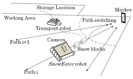
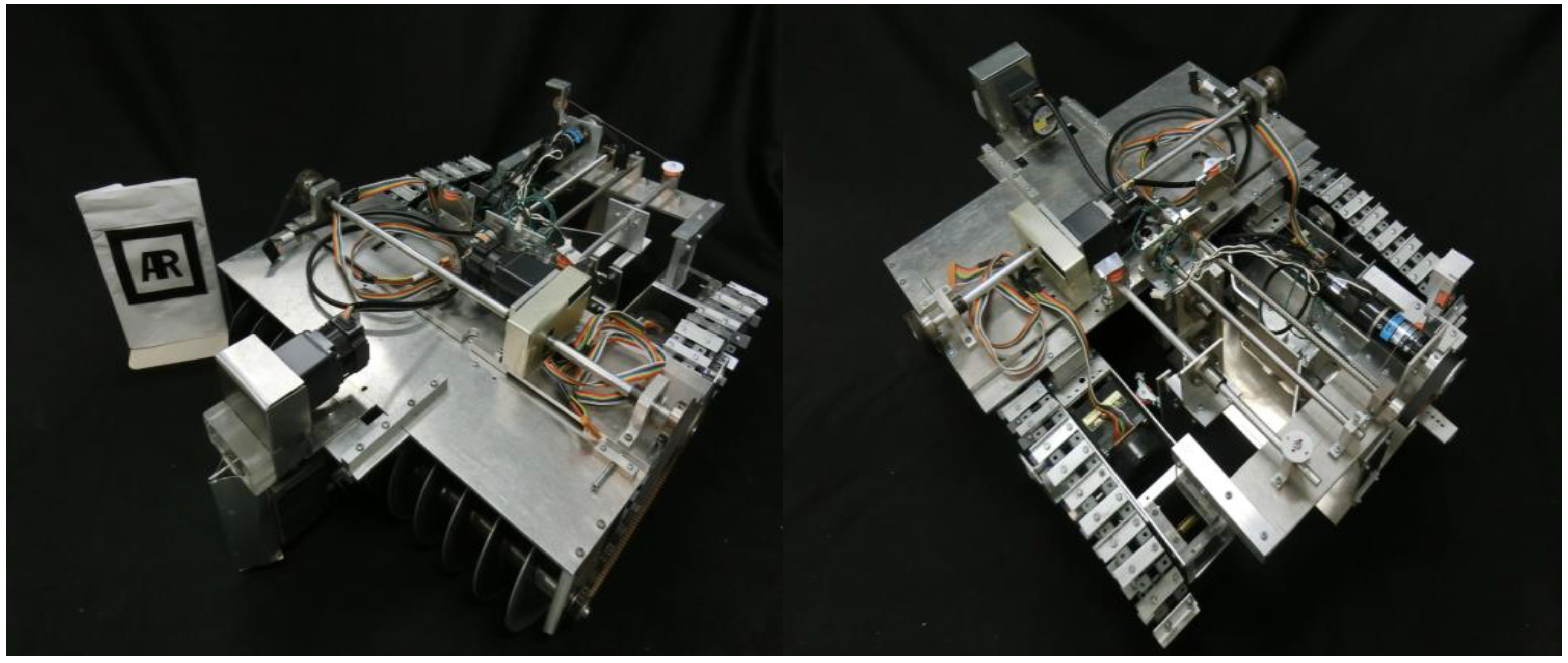
2. Task Overview and Prototype Robots
The SnowEater robot prototype was developed in our laboratory. The prototype is a tracked mobile robot (TMR). Its weight currently is 26 kg, and the size is 540 mm × 740 mm × 420 mm. The main body is made of aluminum and has a flat shape for stability on irregular terrain. The intake system consists of steel and aluminum conveying screws that collect and compact snow at a low rotation speed. Two 10 W DC motors are used for the tracks, and two 15 W DC motors are used for the screws.
The front screw collects snow when the robot is moving with slow linear motion. The two internal screws compact the snow into blocks for easy transportation. Once the snow is compacted, the blocks are dropped out from the rear of the robot. In addition, the intake system compacts the snow in front of the robot reducing the influence of the track sinkage. Since the robot requires a linear motion to collect snow [
5], the path to follow consists of line segments that cover the working area. In our plan, another robot carries the snow blocks to a storage location.
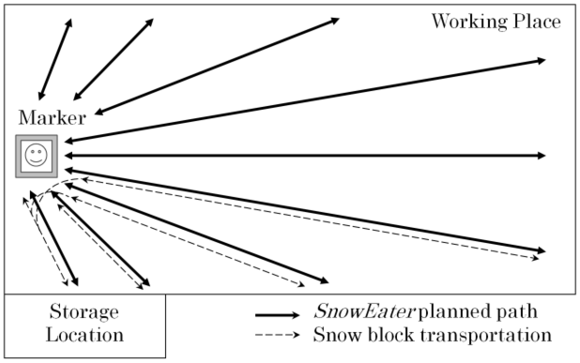
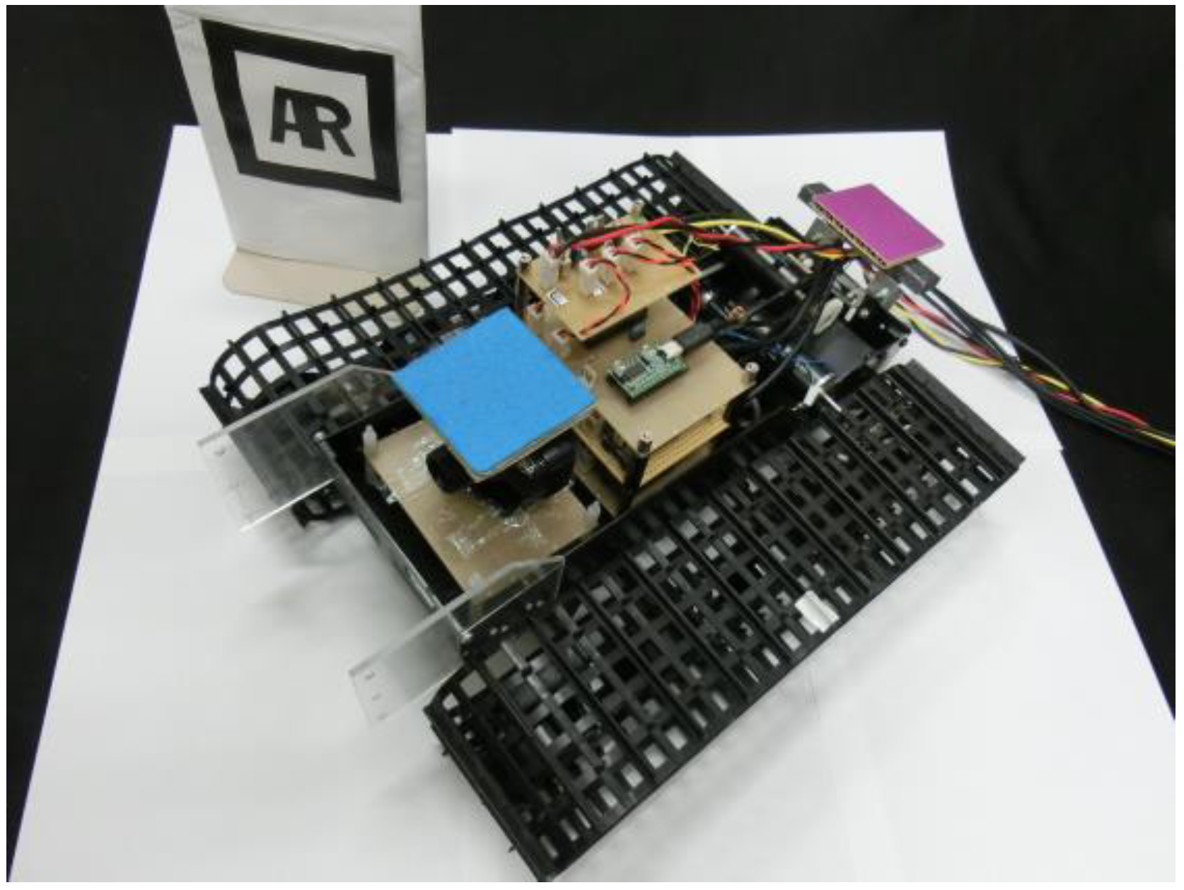
Figure 1 shows the prototype
SnowEater robot, and
Figure 2 shows the line arrangement of the path-following method.
Figure 1.
SnowEater robot prototype.
Figure 1.
SnowEater robot prototype.
Figure 2.
Line paths that cover the snow-removal area.
Figure 2.
Line paths that cover the snow-removal area.
3. Image-Based Navigation System
One of the objectives of the
SnowEater project is to use a low-resolution camera as the sole navigation sensor. In our strategy, a square marker is placed in the center of the working area, so as to be visible from any direction, and a camera is mounted on the robot. Robot camera-marker position/orientation is obtained by using the ARToolKit library [
23]. This library uses the marker four corners position in the camera image and the information given
a priori (camera calibration file and marker size) to calculate the transformation matrix between the camera and marker coordinate systems. Later the transformation matrix is used to estimate the translation components [
24]. However, with low-resolution cameras, the accuracy and reliability of the measurement vary significantly, depending on the camera-marker distance. This is one of the problems associated with localization when using only vision. Gonzales
et al. [
25] discusses this issue and provides an innovative solution using two cameras. A solution for the localization problem using stereoscopic vision is given in [
26,
27], while [
28] presents a solution using rotational stereo cameras. In [
29], a trajectory-tracking method using an inexpensive camera without direct position measurement is presented.
Some studies have utilized different sensors such as a laser scanner to map outdoor environments [
30]. Our study places a high priority on keeping the system as a whole inexpensive and simple; hence the challenge is to exploit robot performance using a low-resolution camera.
In this section, the term “recognized marker position” refers to the marker blob in the captured image, and the term “localization” means identification of the robot location with respect to the marker coordinate system.
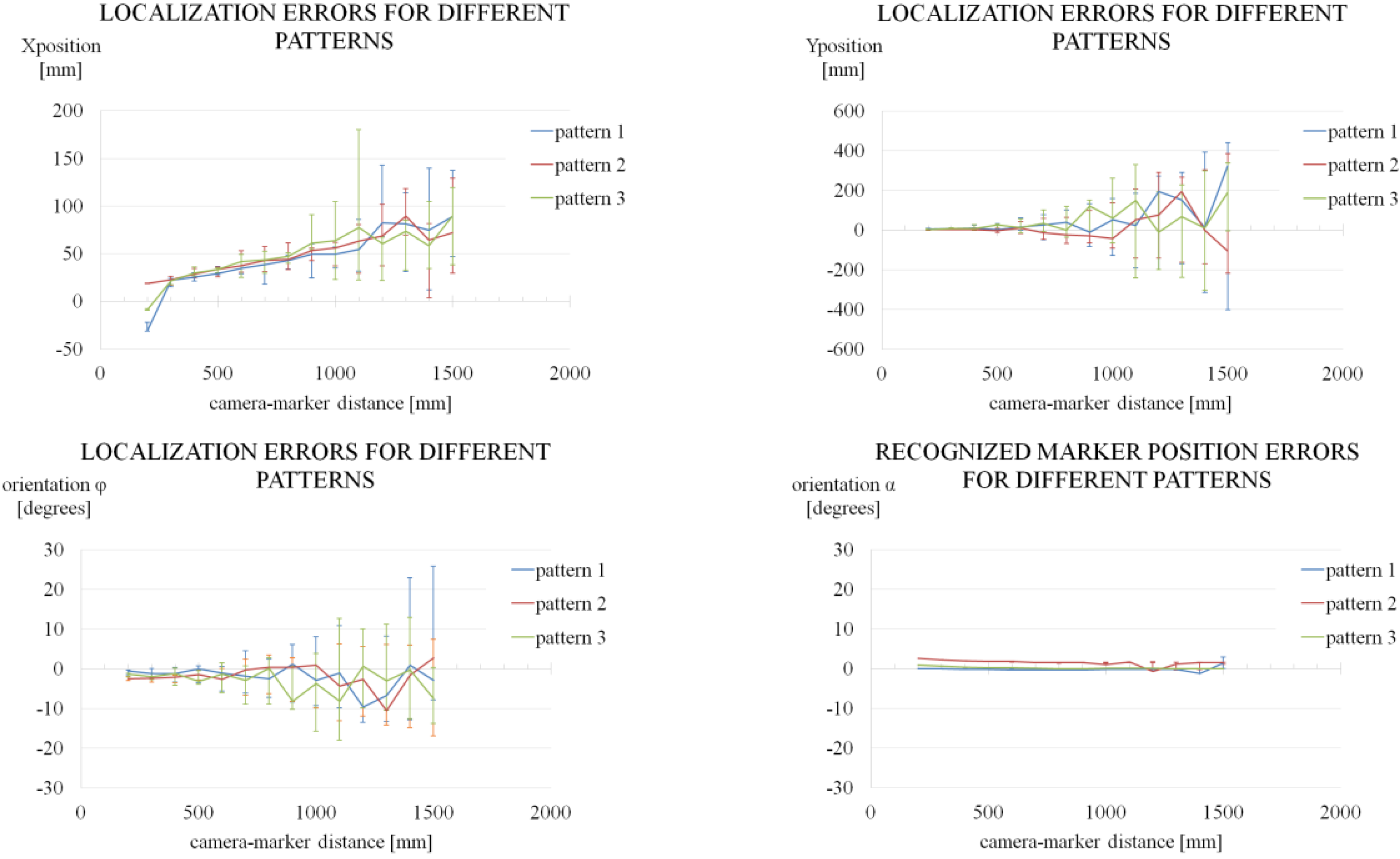
3.1. Localization Performance Evaluation
To evaluate localization performance, outdoor and indoor experiments were carried out using a low-cost USB camera (Sony, PlayStation Eye 640 × 480 pixels) mounted on a small version of the
SnowEater robot. Results with different cameras can be seen in
Appendix A. The dimensions and weight of the small version are 420 mm × 310 mm × 190 mm and 2.28 kg, respectively. Because only a path-following strategy with visual feedback is considered, both robots (
SnowEater and the small version) behave similarly.
Figure 3 shows the small version of the
SnowEater robot.
Figure 3.
Monochromatic square marker and small version of the SnowEater robot.
Figure 3.
Monochromatic square marker and small version of the SnowEater robot.
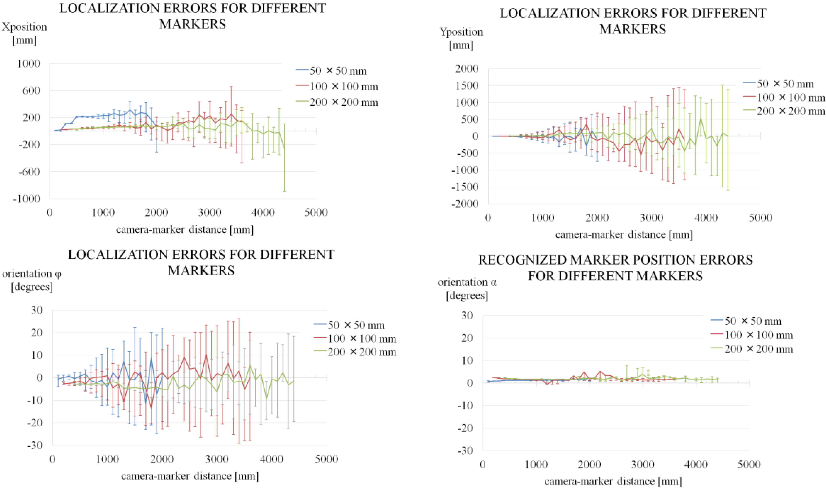
The ARToolKit library uses monochromatic square markers to calculate the camera-marker distance and orientation, and the system can be used under poor lighting conditions [
31]. Our objective is to exploit the library localization merits and performance with low-resolution cameras. Localization control calculations and track commands are completed every 300 ms. Following the results presented in [
6] and
Appendix A, a monochromatic square marker measuring 100 × 100 mm provides enough accuracy to be used in our application; hence the following experiments are done with this marker.
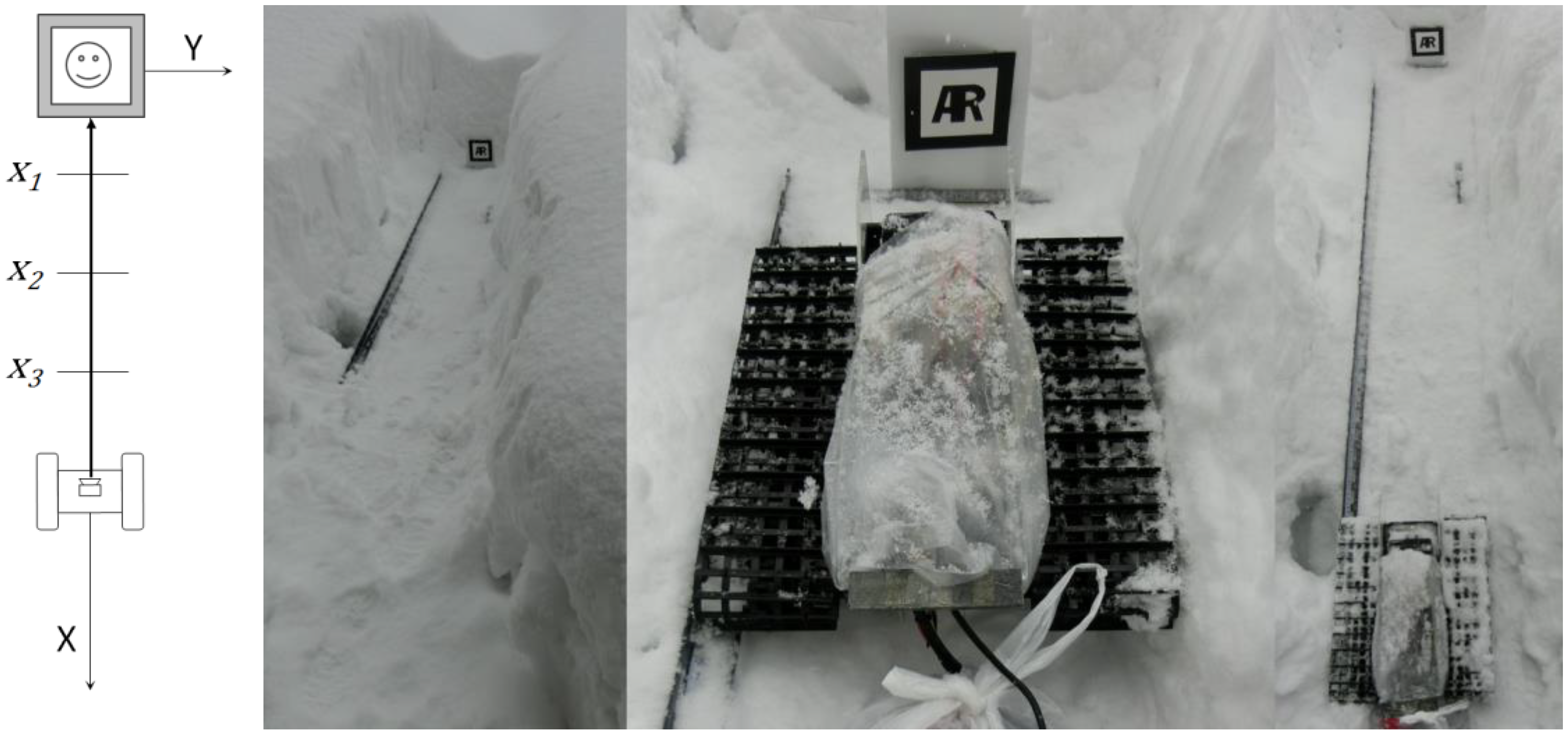
The camera is mounted on the robot facing toward the marker. The robot was placed above the X-axis of the marker-based coordinate system at different
xn positions for 1 min. The outdoor experiment was carried out in snow environments; with air and snow temperatures of −5 °C and −1 °C, respectively.
Figure 4 shows the experimental setup.
Figure 4.
Experimental setup and different camera-marker position during the outdoor experiments.
Figure 4.
Experimental setup and different camera-marker position during the outdoor experiments.
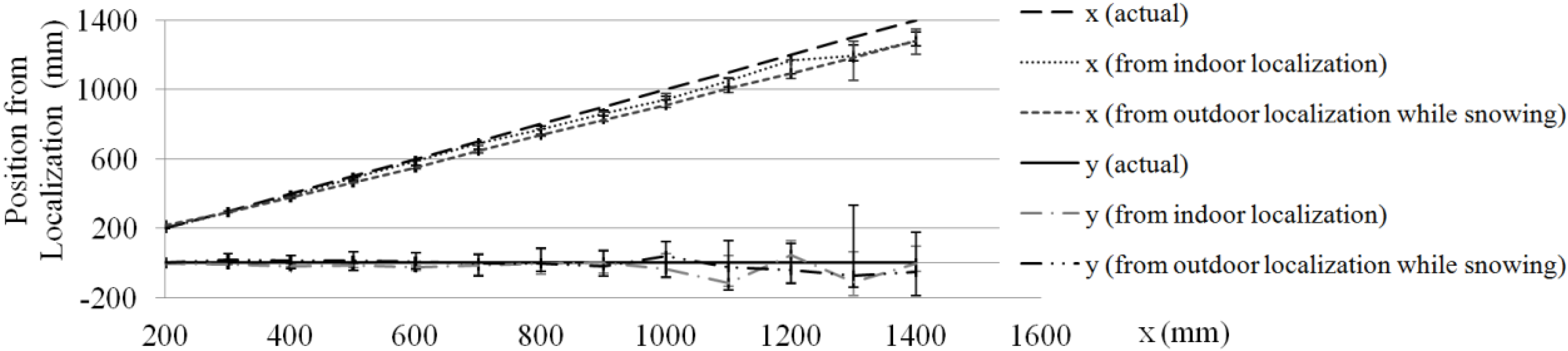
Figure 5 shows the results for the robot position.
Figure 5.
Localization position vs. actual robot-marker distance.
Figure 5.
Localization position vs. actual robot-marker distance.
The results show that the robot x-coordinate is more reliable compared to the y-coordinate. The average values are stable within 800 mm. However, to use the average value the robot must remain in a static state. For motion-state applications, the x-value (camera-marker distance) is more reliable because its variance is smaller than the y-value.
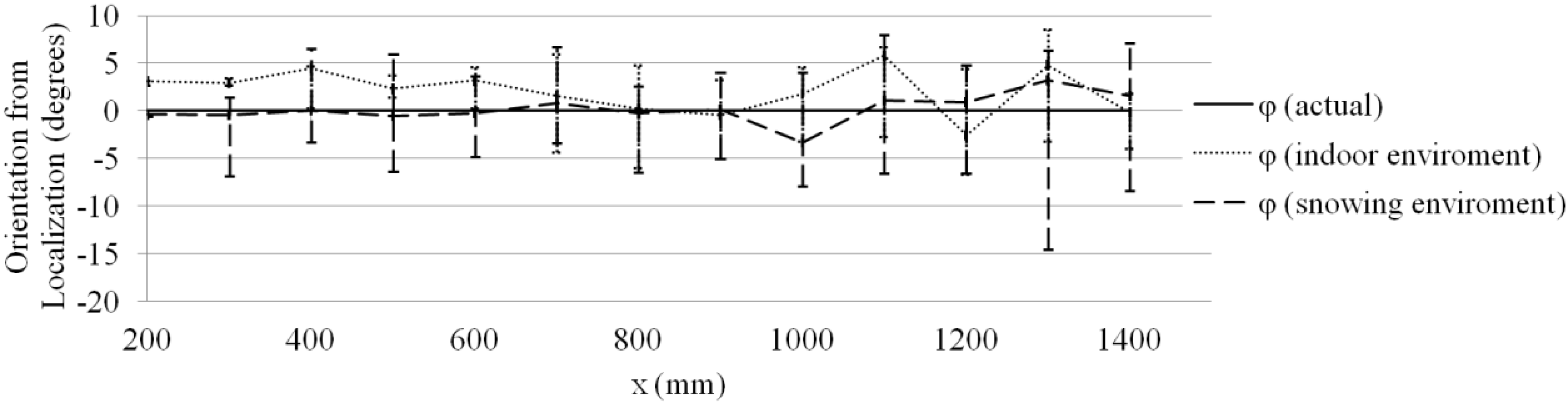
Figure 6 shows the orientation angle experimental results. Since the robot was oriented toward the marker, the angle is 0°.
Figure 6.
Orientation angle vs. robot-marker distance.
Figure 6.
Orientation angle vs. robot-marker distance.
The orientation angle variance increases with the camera-marker distance, and its application is limited to the marker proximity (x < 300 mm) when using a 100 × 100 mm marker.
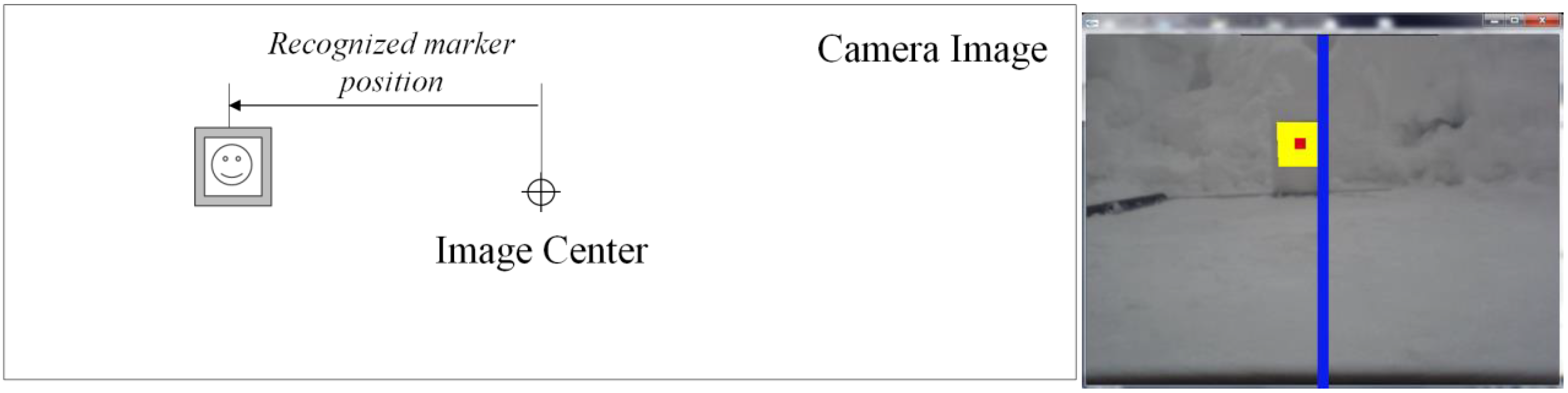
A simple way to obtain the camera-marker direction is to count the number of pixels between the center of the marker blob and the image center in the camera image. These pixel counts are converted into degrees by a simple pixel-degrees relation. This relation is found by finding the number of pixel counts related to a fixed angle.
Figure 7 and
Figure 8 show the results.
Figure 7.
Recognized marker position in the camera image.
Figure 7.
Recognized marker position in the camera image.
Figure 8.
Recognized marker position vs. robot-marker distance.
Figure 8.
Recognized marker position vs. robot-marker distance.
Figure 8 shows the results for the recognized marker position and, as can be seen, there is not a large variance, even when x = 1400 mm. Therefore, the data are reliable and can be used during motion.
In contrast to the orientation results shown in
Figure 6, as the camera-marker distance becomes larger, the recognized marker position error becomes smaller. This characteristic is very useful for our research because the relative angle between the marker direction and robot forward direction can be obtained directly from the image.
In summary, from the controlling perspective, the recognized marker position is reliable when the camera-marker distance is large. When the camera-marker distance is small, localization data can be used. The x-coordinate of the camera-marker distance can be obtained more accurate than the y-coordinate. Based on these properties, a navigation method for distant and vicinity regions can be created.
Section 3.2 describes a novel navigation algorithm based on these properties.
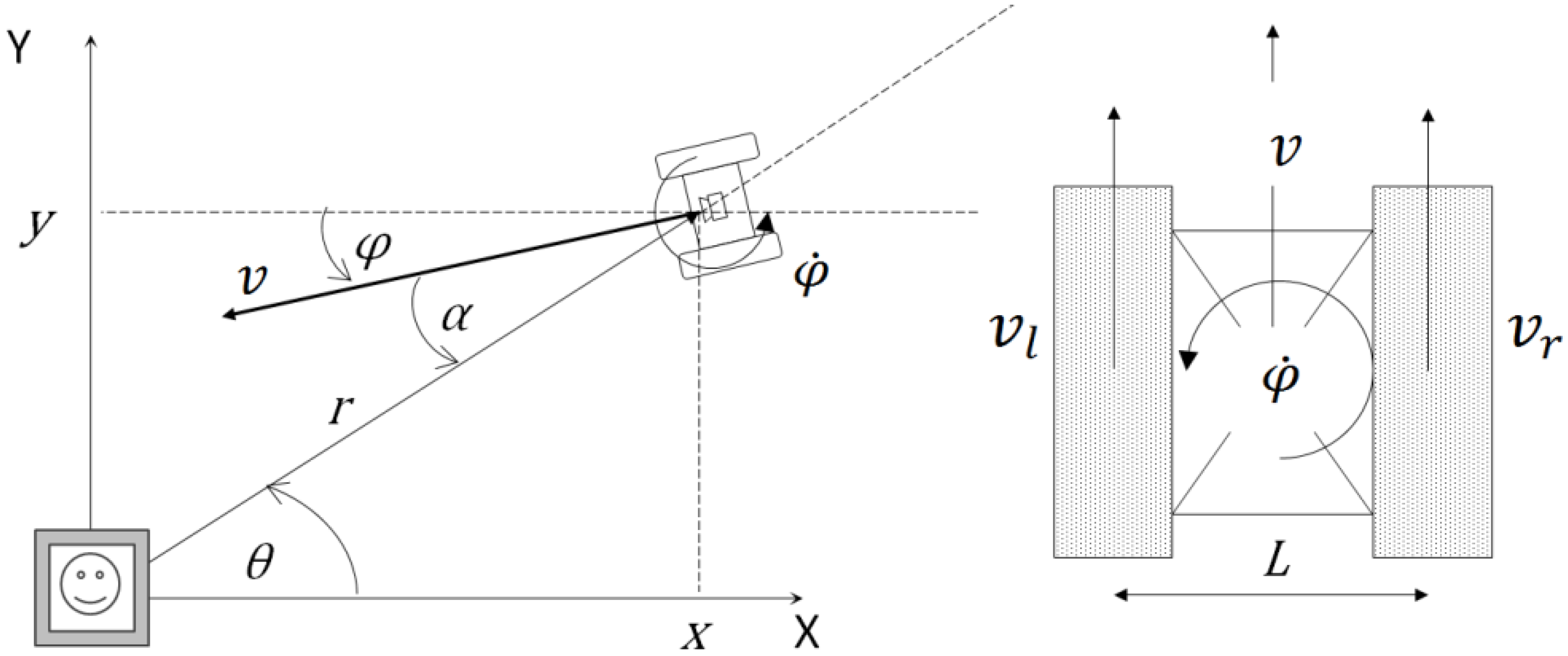
3.2. Motion Model
Although the
SnowEater is a TMR, a differential-drive robot model [
11,
12,
13,
14,
15,
16,
17,
18] is used in the motion algorithm.
Figure 9.
Motion model of the tracked robot.
Figure 9.
Motion model of the tracked robot.
Using the marker coordinate system, the robot coordinates are defined as shown in
Figure 9. The longitudinal and angular velocities of the robot,
and
, are related to the right and left track velocities
and
, respectively, by:
where
represents the distance between the left and right tracks. Among these values,
is used as the control input signal for path following. Velocity
is selected in relation to the snow-processing mechanism of the
SnowEater robot [
5].
Using the robot orientation angle
, the robot velocity in the Cartesian coordinates is expressed as
By differentiating
,
and using Equation (3), the velocity in polar coordinates is expressed as:
where
is the distance from the marker. The relative angle
corresponds to the recognized marker position, and it is used in the motion controller described below.
3.3. Recursive Back-Forward Motion
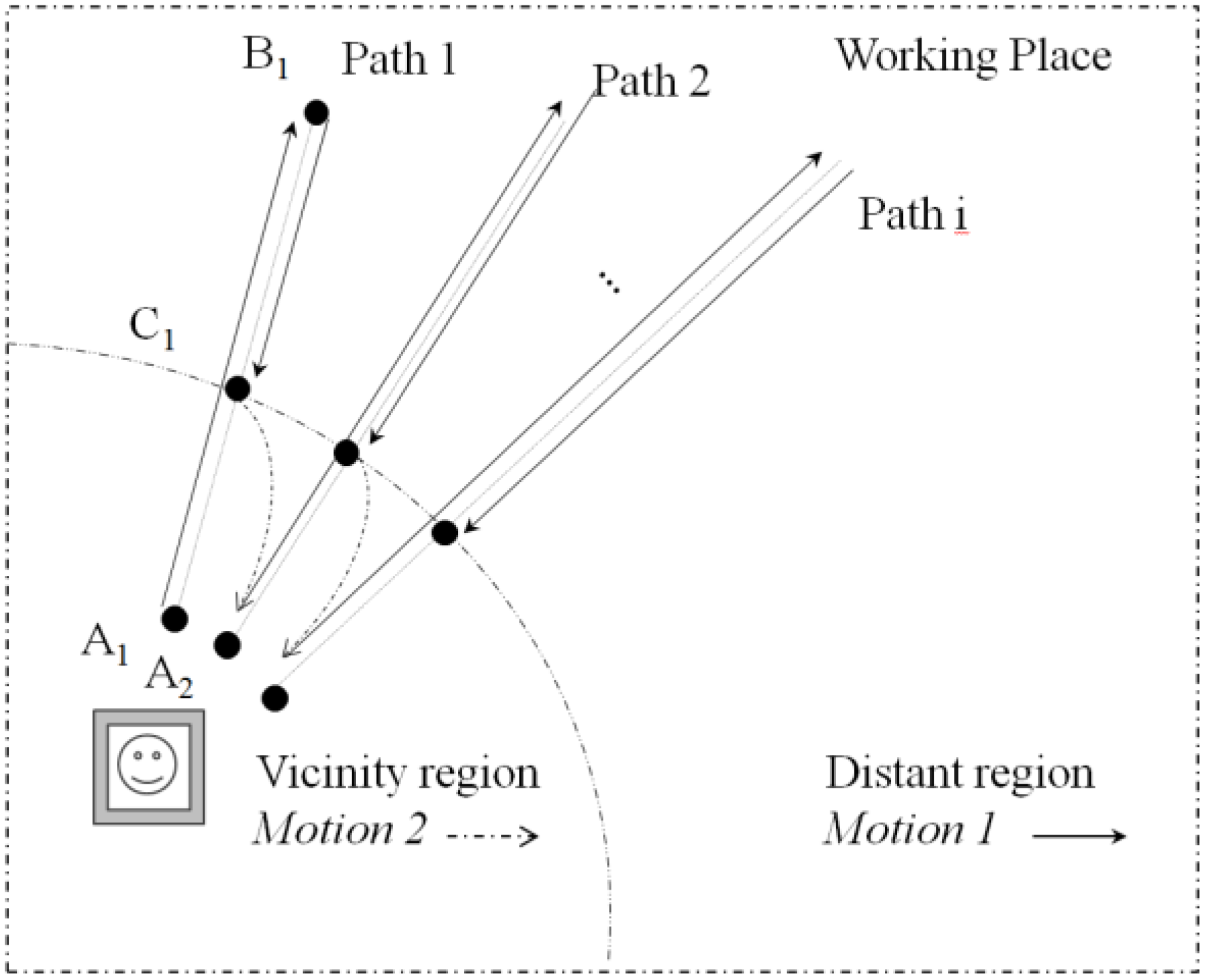
A recursive back-forward motion was created to cover the working area.
Figure 10 shows the travel route of the robot. The robot trajectory consists of two motions:
Motion 1 follows a linear path, while
Motion 2 is used to connect two consecutive linear paths through a curved motion in the vicinity region.
Figure 10.
Recursive back-forward algorithm.
Figure 10.
Recursive back-forward algorithm.
Point A1 is the initial point of the task. The robot moves in the line segment from A1 to B1 using a straight motion (Motion 1). Point B1 is in the limit of the working area in the distant region. After reaching B1, the robot approaches point C1 in the vicinity region using a straight motion (Motion 1). Later, the robot travels to point A2 using a curve motion (Motion 2). Then, the robot embarks upon a new linear path.
Motion 1 control is executed using only the recognized marker position, while Motion 2 uses the distance from the marker in addition to the recognized marker position. With this combined motion, the low-resolution limitation is overcome.
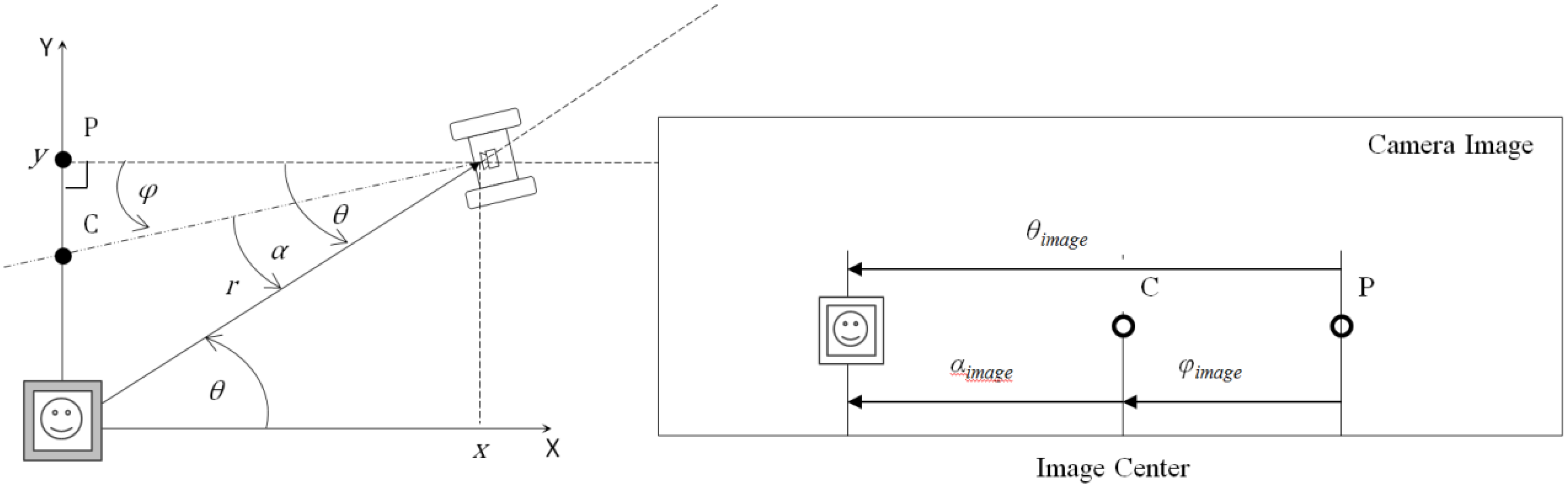
The camera-marker direction is obtained from the information in the image using a geometric relation.
Figure 11 show this relation, where
,
,
are the distance in the camera image corresponding to
α,
θ and
φ.
Figure 11.
Orientation angle of the robot in the marker coordinate system and in the camera image.
Figure 11.
Orientation angle of the robot in the marker coordinate system and in the camera image.
Point C is the image center, which is on a straight heading in front of the robot. Since point P (the projective point of the robot onto the Y axis) is not recognized in the image, the orientation angle is not detected directly in the camera image. Hence the angles and are unknown, even in terms of pixels ( or ) .
However, the relative angle between the marker location and robot direction is available in terms of pixels (). In the following discussion, and are not distinguished.
3.4. Control in Distant Region (Motion 1)
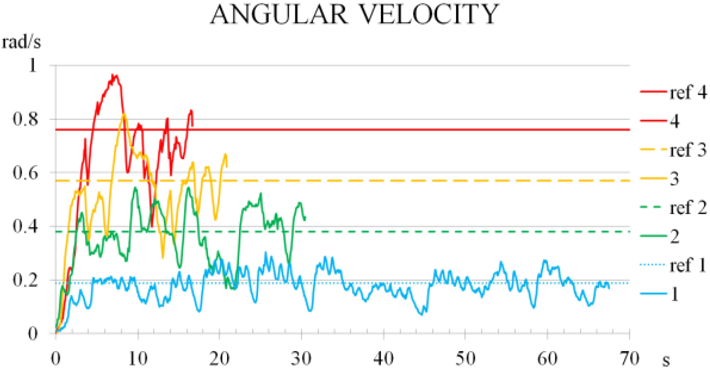
Assuming the track speeds and can be manipulated, the feedback controller is expressed using the angular velocity as the input signal. Throughout the travel, accurate localization can be expected at points A1, C1, A2, C2,…, because of the camera-marker distance.
Motion 1 navigation is executed by a simple direction controller using only the relative angle
in the feedback law.
where
is positive feedback gain. A linear path can be executed when the marker is set to the image center (
). Note this control does not provide asymptotic stability of the target path itself, because the tracking error from the target path cannot be included in control Equation (5) without accurate localization. The path-following error depends on the initial robot position. For this reason, the initial positioning is executed in the vicinity region.
Motion 2 control is described later.
Considering the snow-removal task, this method is a reasonable solution because strict tracking is not required. Moreover, the certainty of returning to the marker position is a good advantage.
The basic property of the direction control used in
Motion 1 is described below. The control purpose is to converge the relative angle
to zero. This convergence can be checked by a Lyapunov function [
32].
By differentiating Equation (6) along the solution of Equations (4) and (5),
A sufficient condition for the negative definiteness of
is:
When the distance
becomes small, the condition is not satisfied. One solution for this issue is to change the velocity as the distance gets smaller to
. Under this condition, Equation (7) becomes:
If there exist
such that
, then:
Therefore, for any
, there exists a time
T such that for all
The reachability of the vehicle to the marker can be understood directly from Equation (4) because the robot is oriented to the marker. The distance
decreases when
. In
appendix C, the behavior of this controller and the conventional PI controller using the available signals is shown.
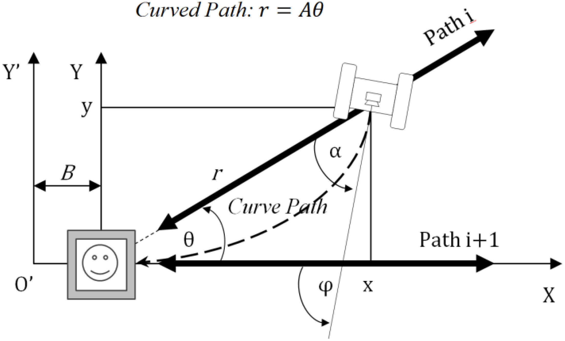
3.5. Control for Switching the Target Line (Motion 2)
In
Motion 2, the robot changes the target path from the current target line (path i) to the next line (path i + 1). During this phase, the robot trajectory is a curve convergent to the next straight target line (path i + 1). To achieve this, a modification is made to feedback Equation (5).
where
is added to change the robot direction. The value of
must be designed to move the robot onto the next target line. We define the value of
as a function of the camera-marker distance (
) as described below.
Considering a polar coordinate system oriented to the next target line (path i + 1), the curved path is defined to satisfy the relation
, where
is a constant. This path smoothly converges to the origin of the O-YX coordinate system. Relying on the good accuracy of the camera localization within the vicinity region, the initial position is assumed to be known.
Figure 12 shows this path.
Figure 12.
Curved path to reach the marker.
Figure 12.
Curved path to reach the marker.
The
A value is selected to create the curved path. Because the initial position is known,
A can be determined. Next,
is related to
by:
Since the robot motion follows Equation (3), the angle
can be expressed as:
if the motion satisfies the relation
Then,
is defined by substituting
and
into Equation (12)
The parameter A has to be selected to satisfy
, because the marker must remain within the camera vision range. In this particular case the vision range is limited and
(because the
y value is small compared to
x). This approximation makes the implementation much easier. Then Equation (16) can be approximated as:
Additionally, the minimum marker recognition distance (
B) must be considered. The coordinate system is shifted from O-YX to O’-Y’X’; hence Equation (17) becomes:
In this method, the asymptotic stability of the path itself is not provided. The stability of the direction control used in
Motion 2 is checked by using a Lyapunov-like function:
By differentiating along the solution of Equation (4) and the feedback equation:
Since for , the error will settle in the region . Hence the expectable accuracy is less than . Note that the error can be suppressed by selecting the correct parameter . The velocity must be small when the robot is closer to the marker to avoid the growth of .
4. Experimental Results
Experimental verification was carried out using the small version of the
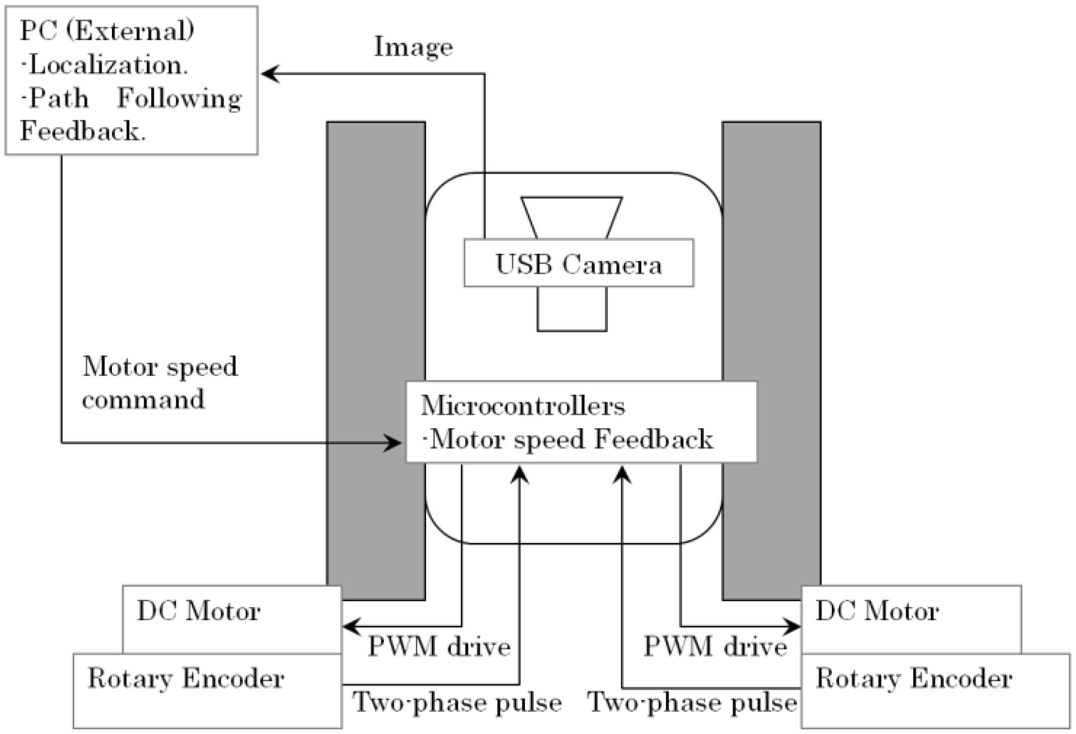
SnowEater robot. The track motors of the small version are Maxon RE25 20 W motors. Each track speed is PI feedback controlled by using 500 ppr rotary encoders (Copal, RE30E) with 10 ms of sampling period. The control signals are sent through a USB-serial connection between an external PC and the robot microcontrollers (dsPIC30F4012). The PC has an Intel Celeron CPU B830 (1.8 GHz) processor with 4 GB of RAM. The interface is made via Microsoft Visual Studio 2010.
Figure 13 shows the system diagram. The track response to different robot angular velocity commands (
) can be seen in
Appendix B.
Figure 13.
Control system diagram for the SnowEater robot.
Figure 13.
Control system diagram for the SnowEater robot.
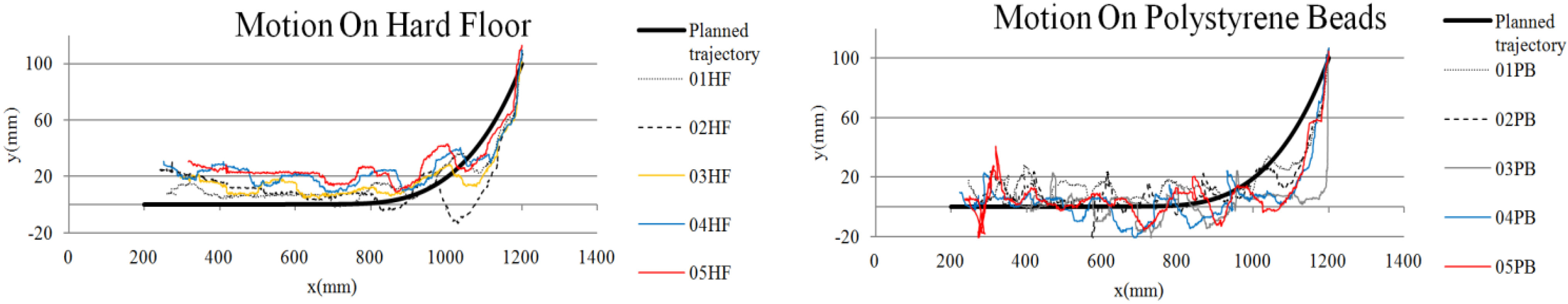
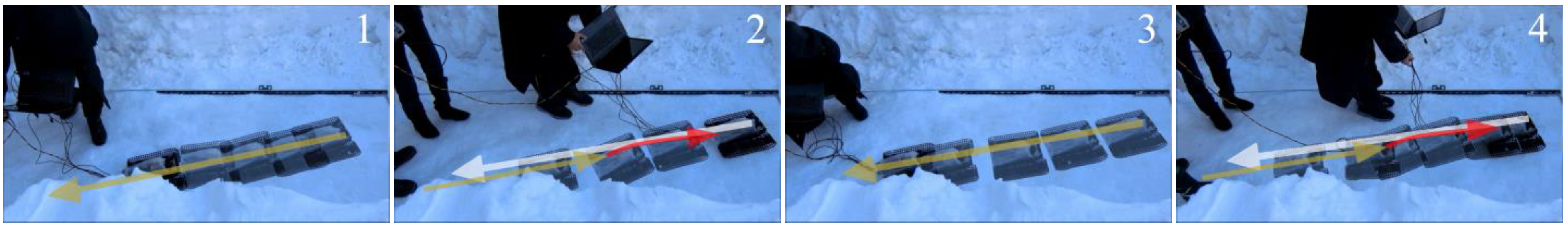
4.1. Motion 2
In this experiment,
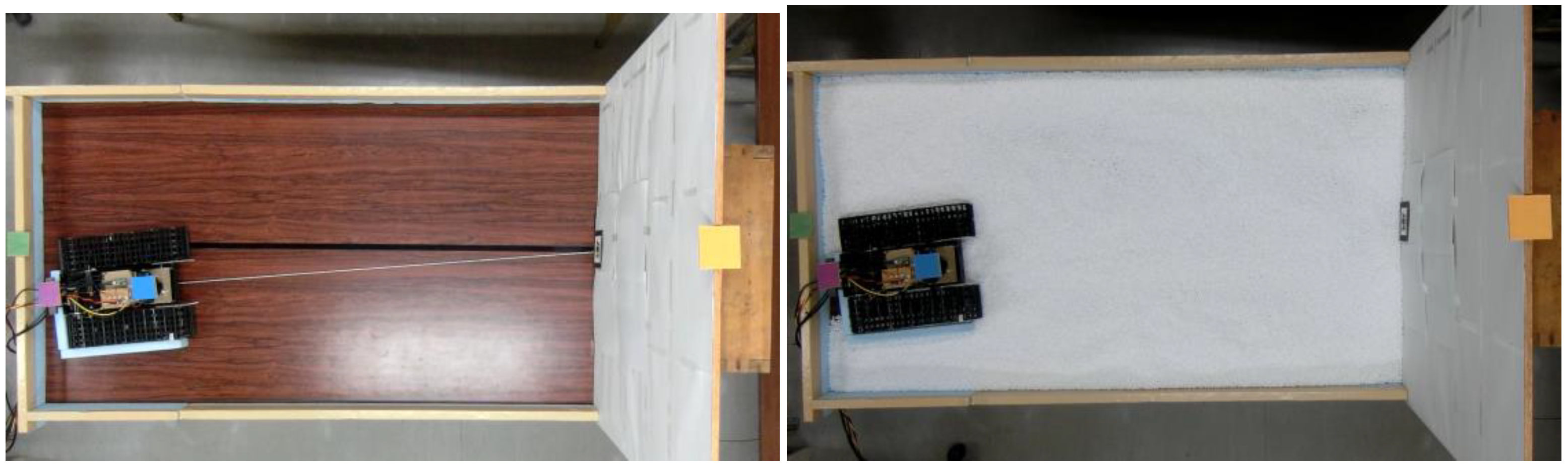
Motion 2 navigation is tested. The control objective is to move the robot to the target line. The experiment is carried out using two different conditions: (1) a hard floor, and (2) a slippery floor of 6 mm polystyrene beads.
Figure 14 shows the experimental setups.
Figure 14.
Motion 2 experimental setup on a hard floor, and on a slippery floor of polystyrene beads.
Figure 14.
Motion 2 experimental setup on a hard floor, and on a slippery floor of polystyrene beads.
The robot position results are obtained using a high-resolution camera mounted on the top of the robot. The robot and marker locations are generated by processing the captured image. The initial position was
xo = 1200 mm,
yo = 100 mm.
Figure 15 and
Figure 16 show the experimental results.
Figure 15.
Robot position throughout the experiment.
Figure 15.
Robot position throughout the experiment.
Figure 16.
experimental results when Motion 2 is executed.
Figure 16.
experimental results when Motion 2 is executed.
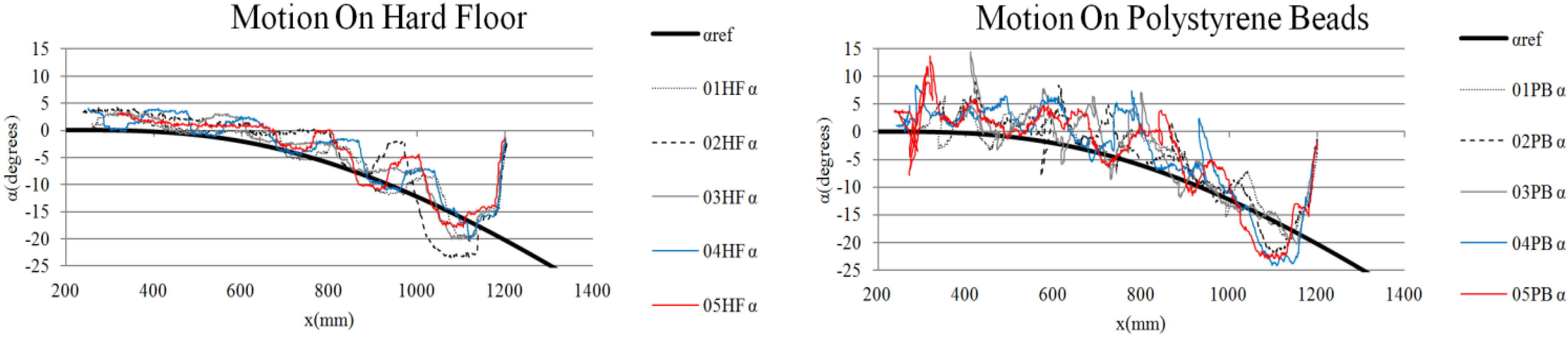
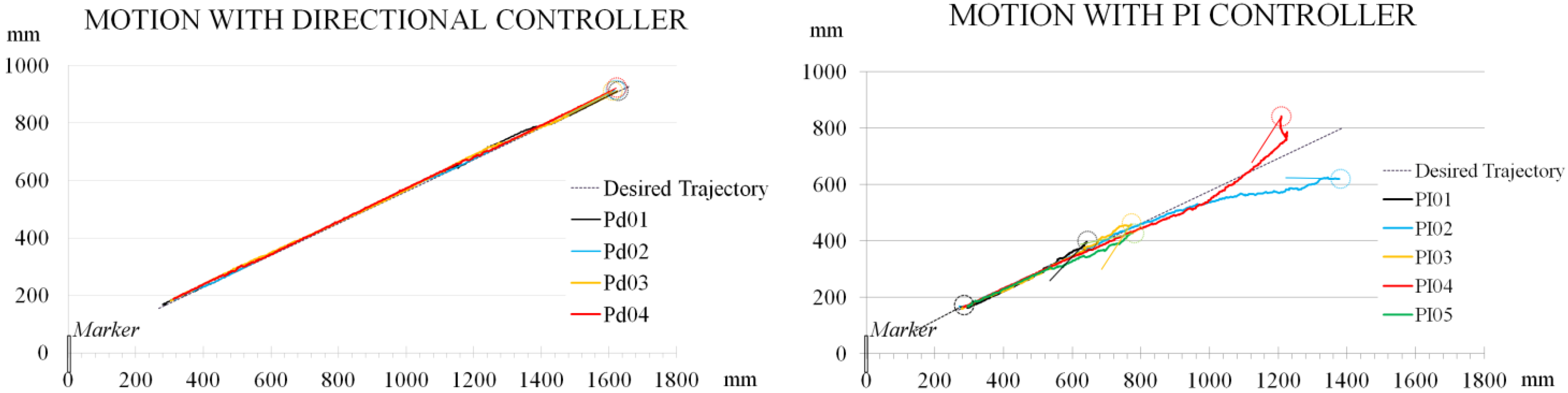
Figure 15 shows a comparison of the
Motion 2 experiment on a hard floor and on polystyrene beads repeated five times.
As
Figure 16 shows, direction control for the angle
is accomplished.
Because the feedback does not provide asymptotic stability of the path to follow, deviations occur in each experiment. If the final position is not accurate, tracking of the path generated by Motion 1 cannot be achieved. If the final error is outside the allowable range, a new curve using the Motion 2 control needs to be generated again. Due to the marker proximity, tracking of the new path is more accurate.
4.2. Motion 1 in Outdoor Conditions
To confirm the applicability in snow environments of this path-following strategy, outdoor experiments were carried out. These experiments were conducted at different times of the day under different lighting conditions.
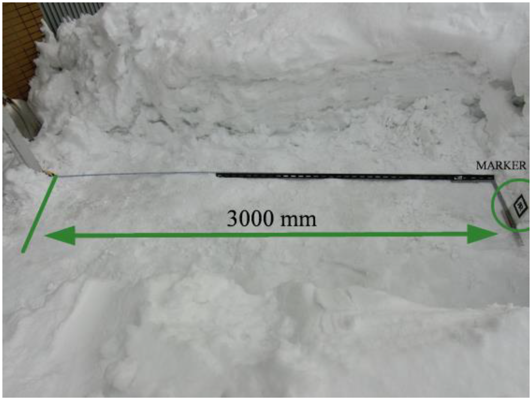
Figure 17 shows the setup of the test area.
Figure 17.
Test area setup.
Figure 17.
Test area setup.
The test area measured 3000 mm × 1500 mm. The snow on the ground was lightly compacted, the terrain was irregular, and conditions were slippery. For the first experiment, the snow temperature was −1.0 °C and the air temperature is −2.4 °C with good lighting conditions.
Figure 18 shows the experimental results for
Motion 1 in outdoor conditions. In both experiments, the robot was oriented toward the marker and the path to follow was 3000 mm long. The color lines in the figures highlight the path followed.
Figure 18.
Motion 1 experimental results on snow in outdoor conditions.
Figure 18.
Motion 1 experimental results on snow in outdoor conditions.
As can be seen in
Figure 18, the robot follows a straight-line path while using
Motion 1.
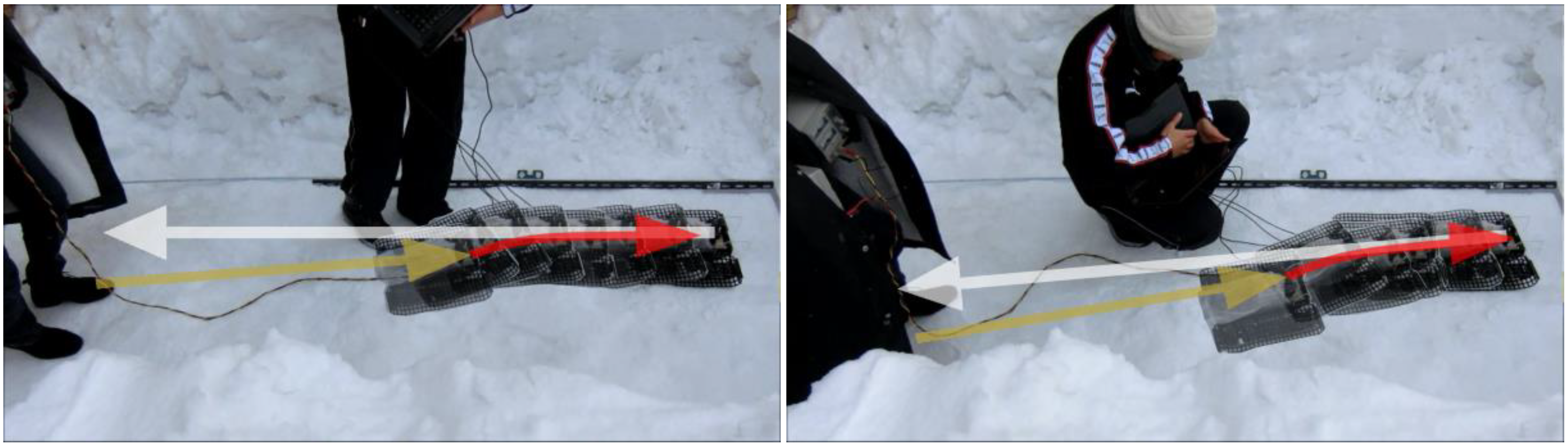
4.3. Motion 2 in Outdoor Conditions
Figure 19 shows the results for the
Motion 2 experiment conducted under the same experimental conditions as for the
Motion 1 experiment. The color lines highlight the previous path (brown), the path followed (red), and the next path (white).
In the left-hand photograph in
Figure 19, the next path is in front of the marker. In the right-hand photograph, the next path has an angle with respect to the marker.
Figure 19.
Motion 2 on snow.
Figure 19.
Motion 2 on snow.
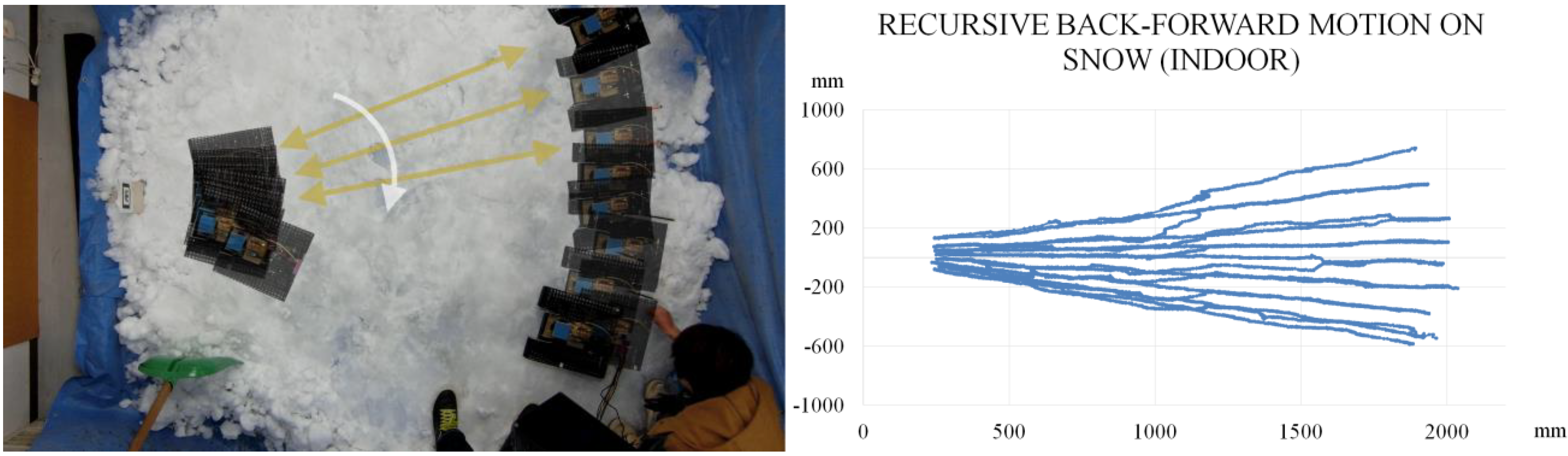
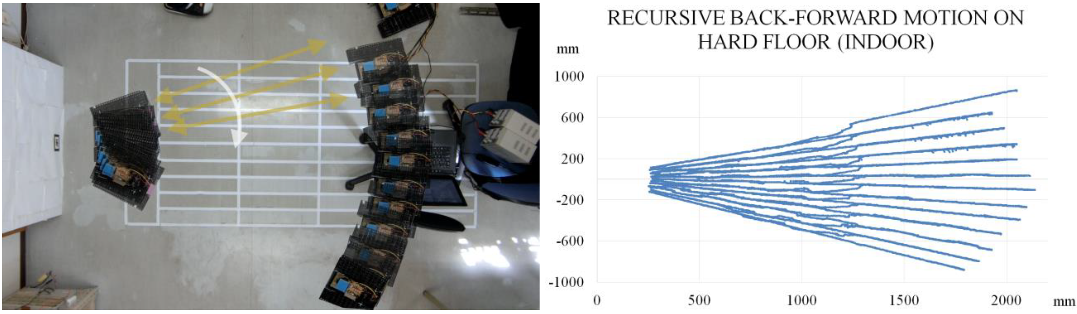
4.4. Recursive Back-Forward Motion
Figure 20 shows the results for the recursive back-forward motion in indoor conditions on a hard floor and on snow. The
Motion 2 region is 1200 mm. The test travelled distance is 2000 mm.
Figure 20.
Recursive back-forward motion experimental results in indoor conditions.
Figure 20.
Recursive back-forward motion experimental results in indoor conditions.
Table 1.
Recursive back-forward motion experimental results in indoor conditions.
Table 1.
Recursive back-forward motion experimental results in indoor conditions.
| | On Hard Floor | On Snow |
|---|
| Reference angle between paths | 4.5° | 4.5° |
| Mean angle between paths | 4.0° | 4.8° |
| Max. angle between paths | 4.6 ° | 6.9 ° |
| Min. angle between paths | 3 ° | 1.6 ° |
| Angle between paths deviation | 0.49° | 1.54° |
The robot covered the testing area using the recursive back-forward motion. For a reference angle of 4.5° between line paths, the average results are: 4° for motion on hard floor and 4.8° for motion on compacted snow. The number of paths in the experiment on snow is different because the test area on snow is smaller than the test area on hard floor. Although the motion performance on snow is reduced (compared to the motion on a hard floor), the robot returned to the marker and covered the area.
Table 1 shows the results of
Figure 20.
In snow removal and cleaning applications, full area coverage rather than strict path-following is required. Therefore, this method can be applied for such tasks.
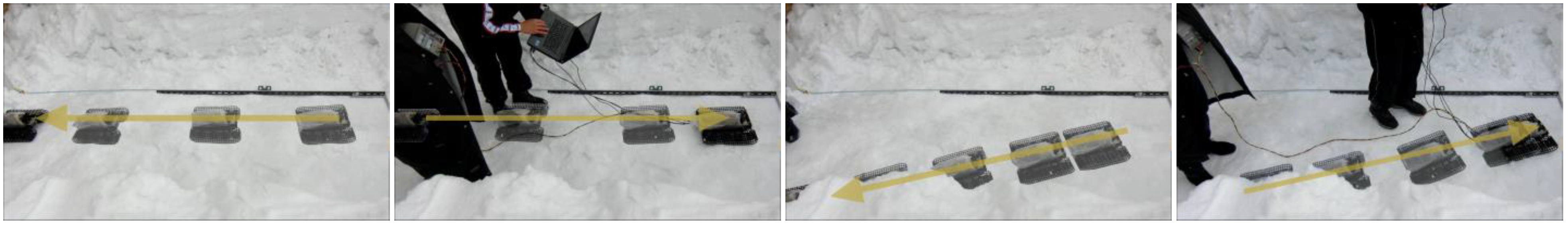
Figure 21 shows the recursive back-forward motion experiment on snow in outdoor conditions. The snow temperature was −1.0 °C and the air temperature was −1.3 °C.
Figure 21.
Recursive back-forward motion experimental results in outdoor conditions.
Figure 21.
Recursive back-forward motion experimental results in outdoor conditions.
Figure 21 results confirm the applicability of the method under outdoor snow conditions. Due to poor lighting, the longest distance traveled was 1500 mm. For longer routes, a bigger marker is required and to improve the library performance in poor lighting conditions, the luminous markers shown in [
31] can be used.
5. Conclusions
In this paper, we presented a new approach for a snow-removal robot utilizing a path-following strategy based on a low-cost camera. Using only a simple direction controller, an area with radially arranged line segments was swept. The advantages of the proposed controller are its simplicity and reliability.
The required localization values, as measured by the camera, are the position and orientation of the robot. These values are measured in the marker vicinity in a stationary condition. During motion or in the marker distant region, only the position of the marker blob in the captured image is used.
With 100 mm × 100 mm square monochromatic marker, a low-cost USB camera (640 × 480 pixels), and the ARToolKit library, the robot followed the radially arranged line paths. For a reference angle of 4.5° between line paths, the average results are: 4° for motion on hard floor and 4.8° for motion on compacted snow. With good lighting conditions, 3000 mm long paths were traveled. We believe with this method our intended goal area can be covered.
Although the asymptotic stability of the path is not provided, our method presents a simple and convenient solution for SnowEater motion in small areas. The results showed that the robot can cover all the area using just one landmark. Finally, because the algorithm grants area coverage, it can be applied not only to snow-removal but also to other tasks such as cleaning.
In the future, the method will be evaluated by using the SnowEater prototype in outdoor snow environments. Also, the use of natural passive markers (e.g., houses and trees) will be considered.


