Development of an Effective Docking System for Modular Mobile Self-Reconfigurable Robots Using Extended Kalman Filter and Particle Filter

Abstract

This paper presents an autonomous docking system with novel integrated algorithms for mobile self-reconfigurable robots equipped with inexpensive sensors. A novel docking algorithm was developed to determine the initial distance and orientation of the two modules, and sensor models were established through experiments. Both Extended Kalman filter (EKF) and particle filter (PF) were deployed to fuse the measurements from IR and encoders and provide accurate estimates of orientation and distance. Simulation experiments were carried out first and then real experiments were conducted to verify the feasibility and good performance of the proposed docking algorithm and system. The proposed system provides a robust and reliable docking solution using low cost sensors.

1. Introduction

Modular and reconfigurable robots (MRR) consist of several modules enabling them to connect to each other to form various configurations. These robots can connect to each other autonomously to form a larger architecture that can perform tasks that one module cannot perform in terms of mobility, power, and functionality [1,2,3,4]. In order to autonomously connect two modules, the docking mechanism usually includes a mechanical system for connecting two modules and a sensing system that estimates the distance and orientations of the two modules.

Various docking mechanisms have been developed, including male-female, gripper, permanent magnet, and electromagnet. For successful autonomous docking, a distance or orientation sensing system is essential. An ultrasonic emitters and receivers have been used in determining the distance and orientation in [5,6]. Ultrasonic sensors are reliable and offer a wide range of measurement distances, but they require a line-of-sight [5]. Also, since they are vulnerable to sound noise, they cannot be used in noisy environments. Kim et al. in [7] estimated distance using RF and used a Kalman Filter (KF) for estimating the position and heading angle. However, authors concluded that extra sensors are required for this sensing system due to its inaccuracy. A camera is used to detect a target using scale-invariant feature transform (SIFT) method [8]. Although SIFT does not need any additional hardware, it has a high computational cost. In [9], a camera and LED lights are used to measure the distance and the orientation of the other module. A vision can also be used to differentiate modules based on color markers on each module [10]. A vision system with color markers does not require high computational power, but light condition and background object color may introduce errors.

Many reconfigurable robots use infrared (IR) emitter-receiver pairs to align their modules for docking due to its low-cost, small size, and low power consumption. The signal strength measurements depend on emitter angle, receiver angle, and the distance [11,12]. The signal strength is the maximum at a given distance when the IR emitter and receiver are aligned. In [13], this property of IR sensor was used to align two modules. However, due to the inaccuracy of the IR sensor, each module keeps rotating for alignment every time the module moves forward a short distance. In [14], the distance between two modules is measured using IR sensors while the orientation of each module is measured using magnetic sensors. However, magnetic sensors must be well calibrated and magnetic field distortion due to the presence of electric devices and ferromagnetic material is also a source of error.

Although accurate sensors are needed for successful docking, they are typically expensive and bulky. Therefore, development of an effective docking algorithm that uses low-cost small size sensors that can provide reliable data is desirable.

This paper presents a novel and robust autonomous docking system that uses EKF to estimate reliable distance and orientation data using low-cost IR emitters, IR receivers, and encoders. In most papers, IR sensors are used to estimate the distance assuming that emitter and receiver angles are close to zero, which often becomes a source of error. This paper presents IR sensor signal strength model based on distance, emitter angle, and receiver angle. Based on the IR sensor model and encoder measurements, an EKF is developed to accurately estimate the distance and angles of the two modules. In addition, an intelligent docking algorithm is developed to align two modules for a successful docking. A permanent magnet and electromagnet connector pair is proposed so that two modules can be docked successfully even with the presence of small offset and misalignment errors. The contributions of this paper lie in: (1) development of EKF and PF algorithms for estimating the position and orientation of autonomous modules; (2) development of a robust docking algorithm for mobile robots; and (3) experimental validation of the proposed system for different case studies, experiments were repeated several times to ensure robustness as well.

The rest of the paper is organized as follows: Section 2 describes the mechanical docking system as well as the sensing system including IR sensor modeling. Section 3 describes the proposed docking algorithm and the proposed EKF and PF algorithms. Section 4 discusses experimental results, while conclusions are provided in Section 5.

2. Docking System

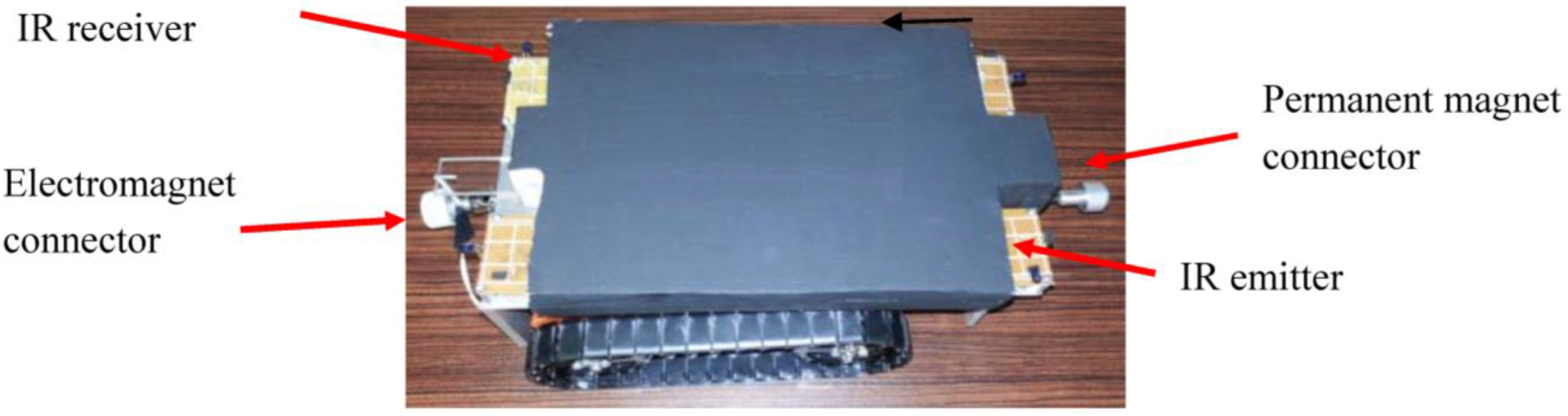
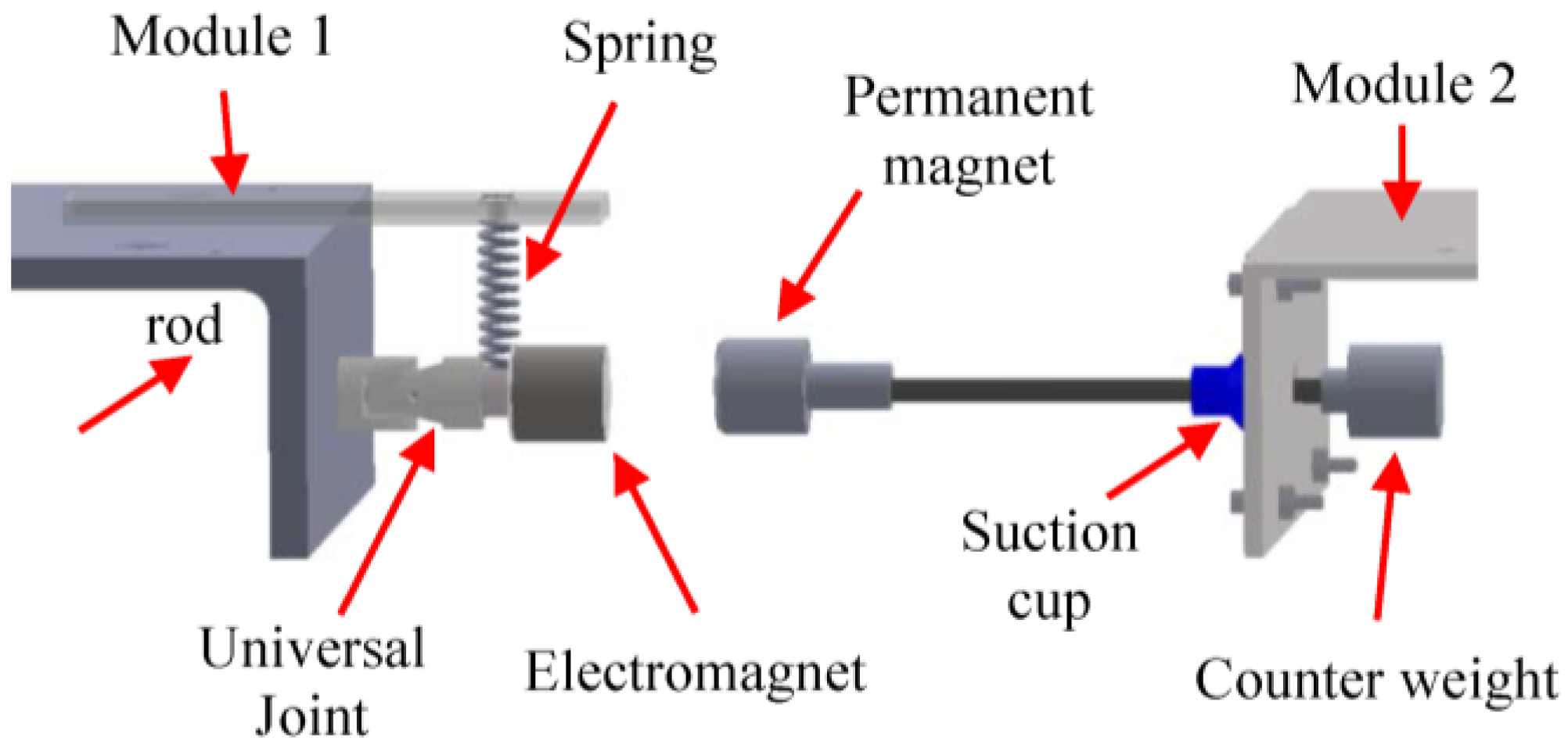
This section discusses the proposed docking mechanism and the associated measurement system. For proper docking, sensors need to be accurately modeled; the sensory data will be used later in the docking algorithm. We first begin this section with introducing the docking mechanism. Next, we present models for the sensors used in this research. Figure 1 shows the proposed modular mobile self-reconfigurable robot. Each module is mobile and equipped with IR emitters and receivers, and encoders. As the docking mechanism, electromagnet and permanent magnet connectors are used.

Figure 1. Proposed modular mobile self-reconfigurable robot with sensing system.

Figure 1. Proposed modular mobile self-reconfigurable robot with sensing system.

2.1. Docking Mechanism

The reliability of the docking mechanism depends on several factors such as rigidity of the connections, error tolerance, and ease of connection/disconnection. To satisfy all the aforementioned factors, electromagnetic solution is considered the most effective mechanism. That is because the magnetic force self-aligns the magnets and also the connection between the modules is rigid. It should be noted that when two permanent magnets are used for docking, it is difficult to disconnect the two modules. Therefore, for easy disconnection, we use a permanent magnet for one side of a connector, and an electromagnet for the other side. This way the modules can be connected or disconnected.

Figure 2 shows our proposed electromagnet and permanent magnet connectors. On the first module (Module 1), a permanent magnet is connected to one side of a module via a long rod supported by a suction cup like a spring. Therefore, the suction cup allows the rod to move freely in two directions allowing the magnet to self-align for docking; the suction cup is also used to center the rod when it is not docked. A long rod is connected to a permanent magnet to compensate large offset errors when the modules are connecting. In order to center the magnet, a counterweight is connected at the other end of the rod. On the other module (Module 2), an electromagnet is connected to a universal joint so that the electromagnet can also move freely in two directions. When permanent magnet and electromagnet are close to each other, can be easily connected even if there is some misalignment and offset.

Figure 2. Proposed magnetic connector.

Figure 2. Proposed magnetic connector.

When the two modules are docked, the electromagnet is powered off, but the two modules stay connected because the permanent magnet attracts the electromagnet. To undock the modules, the polarity of the electromagnet is reversed so that it repels the permanent magnet. Therefore, the electromagnet is only powered during docking and undocking process resulting in small power consumption.

The proposed docking system could adjust up to 25 mm of offset error and 3° of misalignment error. These tolerances can be easily adjusted by changing the permanent magnet or input power to the electromagnet. The next subsection is devoted to the modeling of sensors; these models are used later in the docking algorithm.

2.2. IR Sensor Equation

The IR signal strength depends on the emitter and receiver angles as well as the distance to object. In [12] the IR signal strength was modeled as a function of the distance between emitter and receiver when the two are aligned, i.e.,

$$S\left(L\right)=\frac{a}{L^2}+\mathrm{\beta }$$

(1)

where S is the signal strength, L is the distance between the emitter and the receiver, a is gain, and β is an offset. This offset includes ambient light and can be calculated by taking measurement when the emitter is off. The gain a can be found using a least-square fit method. In [15], both emitter and receiver are placed on the same side to measure the distance between the IR sensor and the object. The IR signal strength with respect to distance and angle was modeled as follows:

$$S\left(L,\mathrm{\theta }\right)=\frac{a}{L^2}\text{cos}\mathrm{\theta }+\mathrm{\beta }$$

(2)

where θ is the incident angle, and β is offset.

Equations (1) and (2) show that IR signal strength diminishes quadratically as the distance between the emitter and the receiver increases. Also, assuming that signal strength is a function of both emitter and receiver angles, the signal strength, $S$, can be modeled as [16]

$$S\left(L,{\mathrm{\theta }}_e,{\mathrm{\theta }}_r\right)=\frac{a}{L^2}\times f\left({\mathrm{\theta }}_e\right)\times f\left({\mathrm{\theta }}_r\right)+\mathrm{\beta }$$

(3)

where $f\left({\mathrm{\theta }}_e\right)$ is a function of emitter angle and $f\left({\mathrm{\theta }}_r\right)$ is a function of receiver angle; emitter and receiver angles are illustrated in Figure 10a. For a successful docking, one needs to accurately measure the distance and orientation between emitter and receiver.

When the connectors are docked successfully, the distance between IR emitter and receiver become 12 cm due to the length of the rod and the universal joint (Figure 2).

Therefore, the IR sensor should have high sensitivity from 12 cm to 20 cm to accurately measure the distance and orientation for docking. To achieve a high sensitivity between 12 cm and 20 cm, the IR emitters should provide high radiant intensity. Also, it is desirable that the intensity measurement changes sharply as emitter or receiver angle changes. To satisfy these two conditions, a TSAL6200 emitter is chosen because it provides high radiant intensity and the angle of half intensity is only 17°. For the receiver, TCRT1000 is used. To model the signal strength as a function of three variables, two variables are kept constants and one variable is changed at a time. Also, the noise of the IR sensor is investigated to evaluate the reliability of the sensor and to incorporate it into the EKF.

2.2.1. Distance Equation

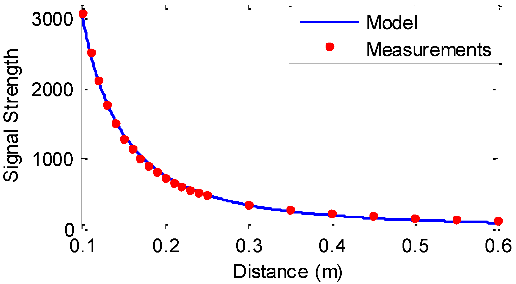
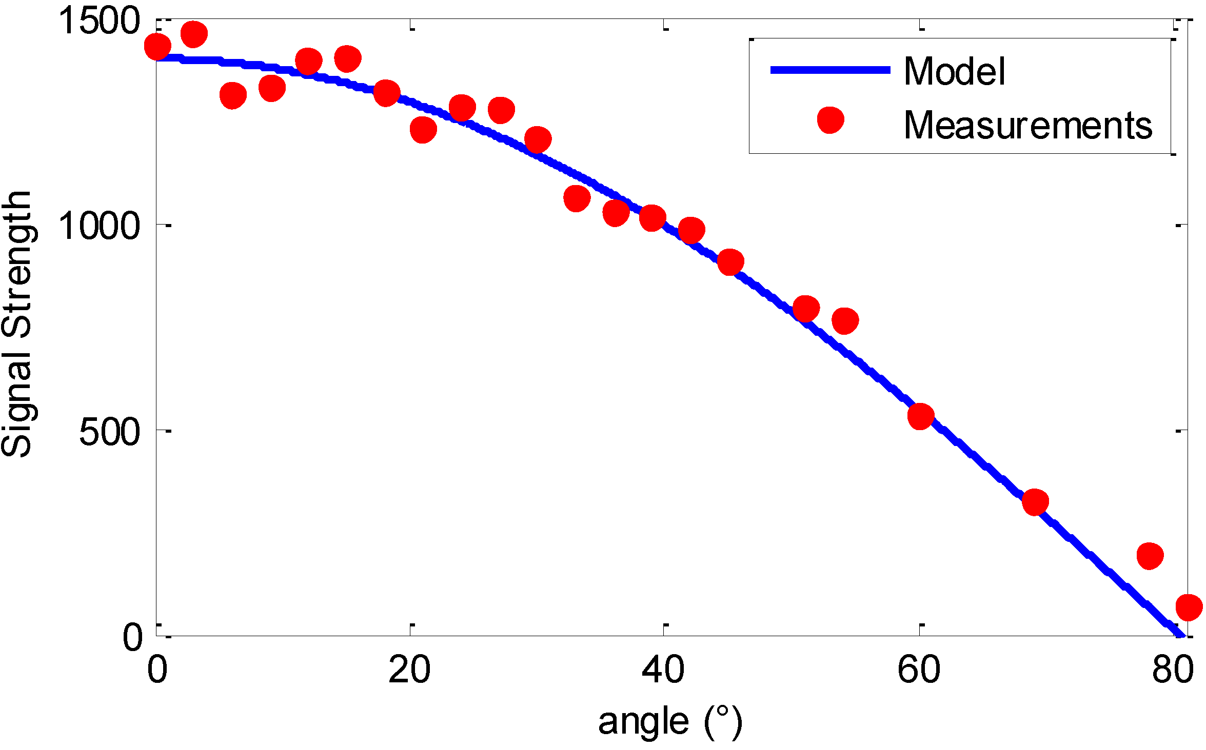
In this section, a model for the distance of IR sensor is developed. To do so, the IR measurements are taken at various distances while the emitter and the receiver are aligned (emitter and the receiver angles at 0°). Then, the signal strength becomes a function of only the distance between the emitter and the receiver. Figure 3 shows the signal strength measurements of the experiment at various distances and the developed distance model using a least square curve fitting.

Figure 3. Signal strength measurements with respect to the distance between IR emitter and receiver and the distance equation when the emitter and receiver angles are 0°.

Figure 3. Signal strength measurements with respect to the distance between IR emitter and receiver and the distance equation when the emitter and receiver angles are 0°.

After compensating for the offset (β), our experimental results verify that the relationship between the distance and signal strength is:

$$S(L)=\frac{31.5}{L^2}$$

(4)

The signal strength is digital measurement (from 0 to 4095), thus does not have any unit. As can be seen in Figure 3, the equation matches the measurements very well.

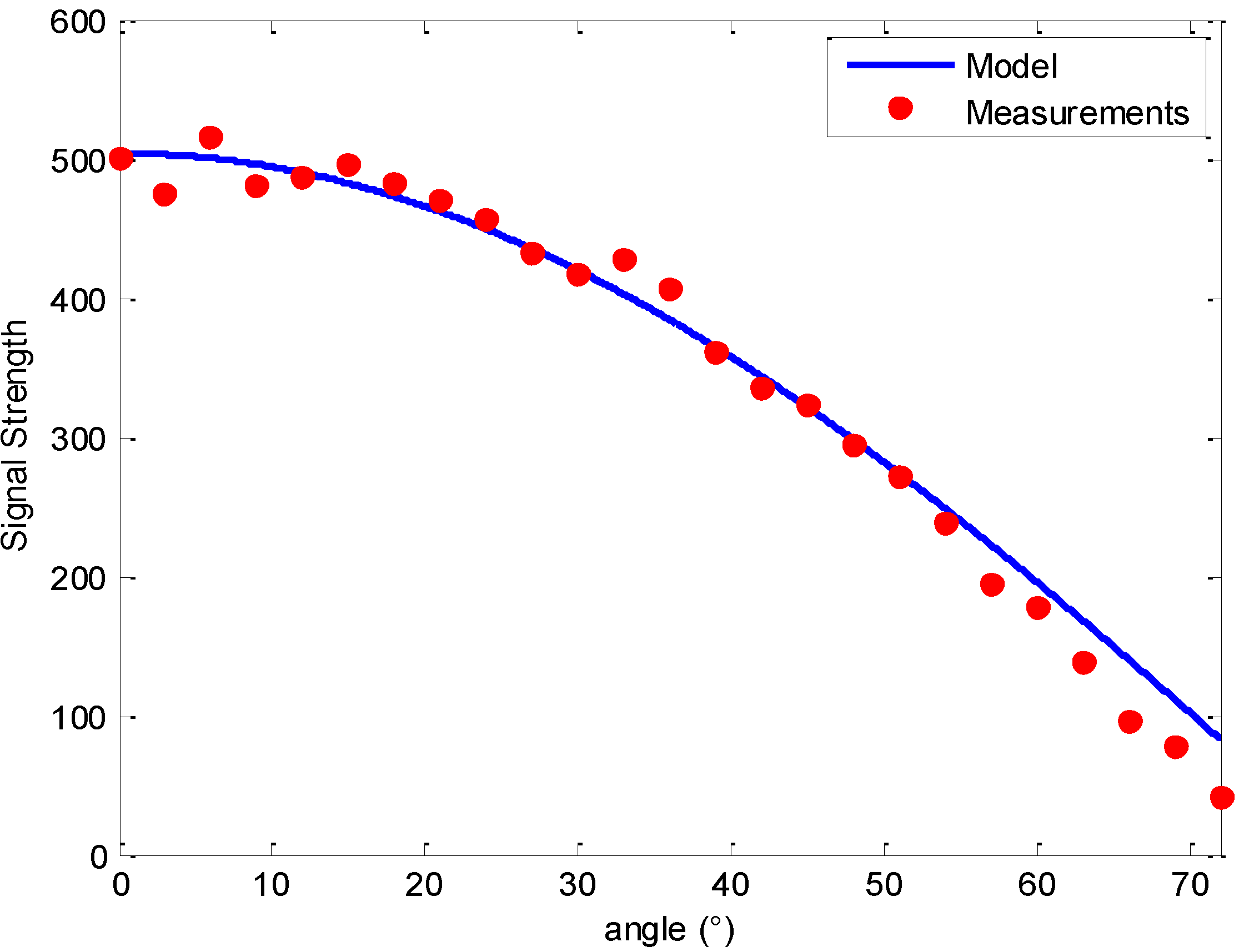
2.2.2. Receiver Angle Equation

This section discusses the modeling of the receiver angle. For this purpose, the emitter angle is fixed at 0° and the distance is fixed at 15 cm and 25 cm. The measurements and the model with different distance are shown in Figure 4 and Figure 5.

The distance equation was also incorporated into the equation of the signal strength as a function of the receiver angle. The relationship between the receiver angle (${\mathrm{\theta }}_r$), distance (L), and signal strength (S) measurement is obtained as

$$S(L,{\mathrm{\theta }}_r)=\frac{31.5}{L^2}\times \cos (1.12{\mathrm{\theta }}_r)$$

(5)

where ${\mathrm{\theta }}_r$ is the receiver angle (radian). Both Figure 4 and Figure 5 show that the measurements match well with the equation given in Equation (5).

Figure 4. Signal strength with respect to the receiver angle measurements and the receiver at the distance of 15 cm.

Figure 4. Signal strength with respect to the receiver angle measurements and the receiver at the distance of 15 cm.

Figure 5. Signal strength with respect to the receiver angle measurements and the receiver at the distance of 25 cm.

Figure 5. Signal strength with respect to the receiver angle measurements and the receiver at the distance of 25 cm.

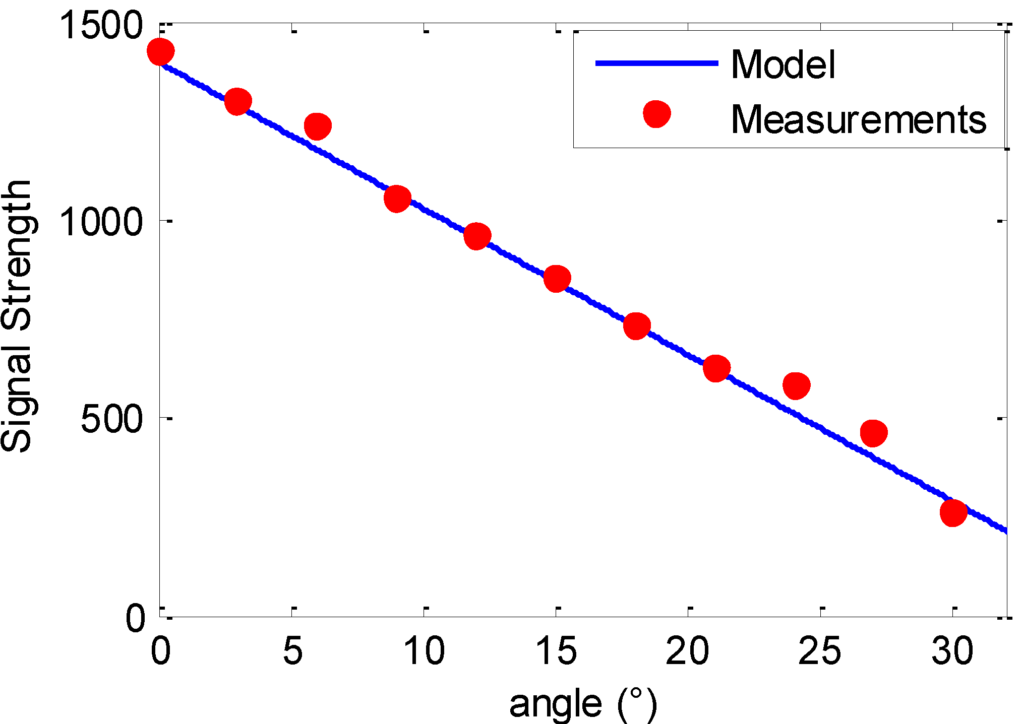
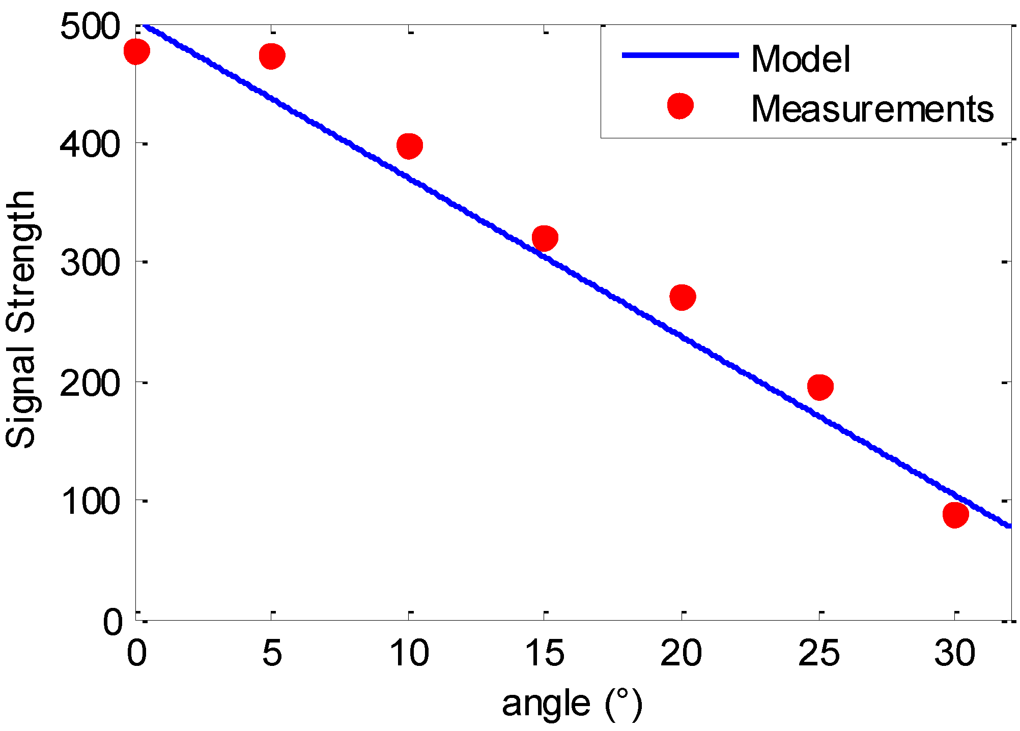
2.2.3. Emitter Angle Equation

In this section, the signal strength is modeled with respect to the emitter angle. To do so, the receiver angle is fixed at 0° and the distance is fixed at 15 cm and 25 cm. The experiment results show that signal strength decreases linearly as the emitter angle increases. The relationship between the emitter angle (${\mathrm{\theta }}_e$) and signal strength (S) measurement used for the model is obtained as

$$S(L,{\mathrm{\theta }}_e)=\frac{47.7}{L^2}(0.66-{\mathrm{\theta }}_e)$$

(6)

where ${\mathrm{\theta }}_e$ is emitter angle in radian. Since a linear equation with an offset is used, the estimated constant value is changed from 31.5 to 47.7, which is 31.5/0.66. The signal strength measurements and the model obtained are shown in Figure 6 and Figure 7.

Figure 6. Signal strength with respect to the emitter angle measurements and the emitter model at the distance of 15 cm.

Figure 6. Signal strength with respect to the emitter angle measurements and the emitter model at the distance of 15 cm.

Figure 7. Signal strength with respect to the emitter angle measurements and the emitter at distance of 25 cm.

Figure 7. Signal strength with respect to the emitter angle measurements and the emitter at distance of 25 cm.

Equations (4)–(6) are now combined to model the signal strength as a function of distance, emitter angle, and receiver angle as:

$$S(L,{\mathrm{\theta }}_r,{\mathrm{\theta }}_e)=\frac{47.7}{L^2}\cos (1.12{\mathrm{\theta }}_r)(0.66-{\mathrm{\theta }}_e)$$

(7)

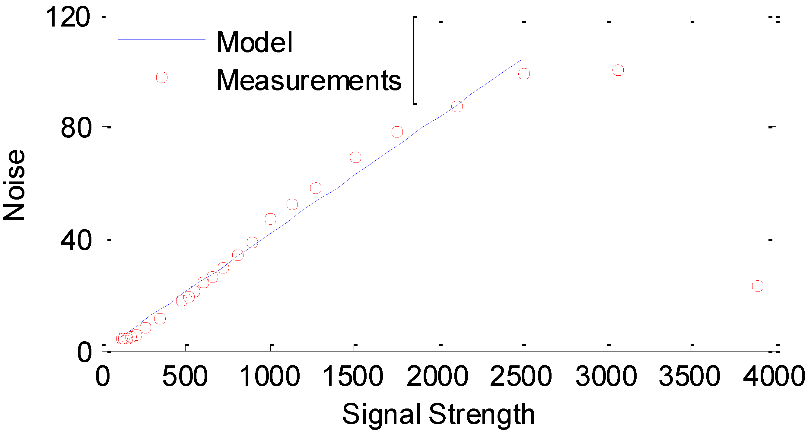
2.2.4. Noise

We need to measure the IR sensor noise to evaluate the reliability of the sensor. We performed experiments where the results are shown in Figure 8. The measurements show that the noise increases almost linearly until signal strength is increased to 2500. Thus, the noise up to this region is modelled linearly. The noise measurements also show that when the signal is greater than 2500, the signal noise does not increase significantly and decreases when signal strength increases even further. For this application, the maximum signal strength measurement is 2200, which is measured when the IR emitter and receiver are 120 mm apart with 0° misalignment (Figure 3). Thus, we use a linear model for the noise.

Figure 8. Root Mean Square (RMS) noise measurements.

Figure 8. Root Mean Square (RMS) noise measurements.

3. Development of Docking Algorithm and State Estimators

In this section, we present a docking algorithm for two robot modules. To perform a successful docking our algorithm requires accessing the distance and angles of modules with respect to each other. Using “direct” sensory data is not possible because of inherent noise in sensors. We therefore, design estimators to estimate the required states (distance and orientation) for docking. Thus, we present our docking algorithm in Section 3.1. Next, we present the state estimators in Section 3.2.

3.1. Docking Algorithm

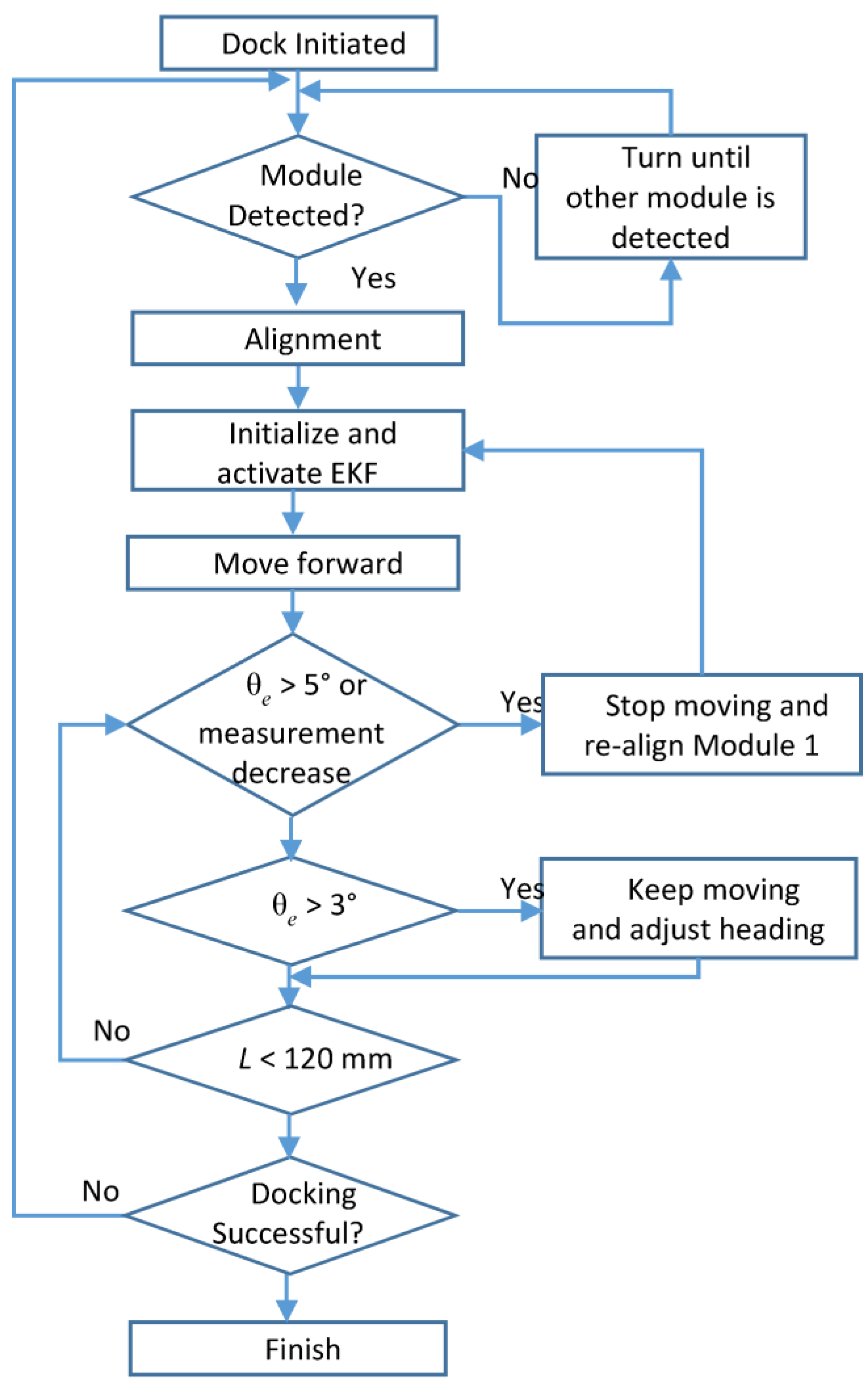
The proposed docking algorithm aligns two modules, determines the initial state, and check if the docking is successfully achieved (without using any extra sensors such as a limit switch). The docking algorithm is illustrated in Figure 9. The details of the algorithms are as follows:

• When the docking is initiated, each module sends the IR signals to search for the other module.
• Module 1 keeps rotating until it is approximately aligned with Module 2. To check for the alignment, the system detects if the signal strength decreases four consecutive times or it is 80% of the maximum measured signal strength. When Module 1 is approximately aligned, Module 1 rotates in the opposite direction to compensate for the overshoot. Then, Module 1 stops and sends signals to Module 2 using the IR emitter to indicate its approximate alignment with Module 2.
• For a fine alignment, IR measurements of Module 2 are used instead of Module 1 because signal strength decrease due to emitter angle changes (Figure 5) is much steeper compared to the receiver angle change (Figure 4) especially for small angles. When the IR signal strength of Module 2 decreases four consecutive times or the signal strength is 90% of the maximum measured signal strength, Module 2 signals Module 1 to stop rotating because Module 1 is now aligned with a small overshoot. Then, Module 1 rotates in the opposite direction for a short period of time to compensate for the overshoot.
• After Module 1 is aligned, Module 2 is aligned using the same procedure (Step 2 to 3).
• After modules are aligned, the distance between the two modules can be estimated using Equation (7).
• Module 1 keeps moving forward. The state estimator is activated every time the encoder count exceeds a certain threshold.
• If the emitter angle (θ_e) > 5° or IR measurement decreases, the initial estimation is most likely incorrect. In these cases, Module 1 stops moving forward and re-aligns. Then, the initial state is recalculated.
• When the estimation of the emitter angle is 3° < θ_e < 5°, Module 1 adjusts the heading angle so that θ_e < 3° while moving forward.
• If the distance, L, is less than 120 mm, which is the length of the docking part, Module 1 moves backwards for 3 seconds to check if docking is successful. If docking is successful, IR signal strength is high. Otherwise, IR signal strength is low because only Module 1 is moved backwards, which results in longer distance between the two modules. In this case, the docking procedure is repeated from Step 2.

State Estimators

Since the IR signal strength is a function of three different variables, it is difficult to accurately estimate distance between two modules especially from noisy measurements. Encoders can also be used to estimate the travelled distance and heading angle of a module, but it is not accurate due to wheels slippage, which accumulates the error over time especially for a mobile robot using a skid-steering system. To estimate distance and orientation more accurately from noisy IR sensor and inaccurate encoder measurements, an EKF and a PF are developed to estimate the required states. This section presents the development of the EKF and PF to estimate the distance and orientations of the modules using IR sensors and encoders. To use the state estimators more effectively, an efficient docking algorithm that aligns the two modules are proposed.

KF and EKF are widely used to estimate the position and orientation [17,18]. They combine multiple sensor measurements to achieve higher accuracy than using single sensor measurements. A KF is used to estimate states of linear models, and an EKF is used for nonlinear models. Since Equation (7) is nonlinear, an EKF should be used.

Figure 9. The Flow chart of the docking algorithm.

Figure 9. The Flow chart of the docking algorithm.

An EKF has two stages, prediction and update. Prediction stage predicts the next state using previous state estimate, input to the system, and the system model. Update stage corrects the prediction using measurements. Consider the following nonlinear state space model in a discrete time:

$$x_k=f_k\left(x_{k-1},u_{k-1}\right)+w_{k-1}$$

(8)

$$z_k=h_k\left(x_k\right)+v_k$$

(9)

where subscript k represents iteration count, $x_k$ is the state, ${\mathrm{f}}_{\mathrm{k}}$ is a state transition function from time ${\mathrm{t}}_{\mathrm{k}-1}$ to time ${\mathrm{t}}_{\mathrm{k}}$, ${\mathrm{u}}_{\mathrm{k}-1}$ is the deterministic input, ${\mathrm{w}}_{\mathrm{k}-1}$ is the process noise, ${\mathrm{z}}_{\mathrm{k}}$ is the measurement, ${\mathrm{h}}_{\mathrm{k}}$ is a measurement function, and ${\mathrm{v}}_{\mathrm{k}}$ is the measurement noise. In order to use an EKF, the system models should be linearized using the first order Taylor series expansion. Let the first order Taylor series expansion of the nonlinear function ${\mathrm{f}}_{\mathrm{k}}\left({\mathrm{x}}_{\mathrm{k}-1},{\mathrm{u}}_{\mathrm{k}-1}\right)$ and ${\mathrm{h}}_{\mathrm{k}}\left({\mathrm{x}}_{\mathrm{k}}\right)$ be ${\mathrm{A}}_{\mathrm{k}}$ and ${\mathrm{C}}_{\mathrm{k}}$, respectively. Then, ${\mathrm{A}}_{\mathrm{k}}$ and ${\mathrm{C}}_{\mathrm{k}}$ become

$$A_k={f_k}^{\prime }\left(x_{k-1},u_{k-1}\right)=\frac{\partial f_k(x_{k-1},u_{k-1})}{\partial x_{k-1}}$$

(10)

$$C_k=h_k^{\prime }\left(x_k\right)=\frac{\partial h_k\left(x_k\right)}{\partial x_k}$$

(11)

Then, the state can be estimated as follows:

Prediction:

$${\widehat{x}}_k^{-}=f_k({\widehat{x}}_{k-1}^{+},u_{k-1})$$

(12)

$$P_k^{-}=A_k\cdot P_{k-1}^{+}\cdot A_k^T+Q_{k-1}$$

(13)

Update:

$$K_k=P_k^{-}\cdot C_k^T\cdot {[C_k\cdot P_k^{-}\cdot C_k^T+R_k]}^{-1}$$

(14)

$$P_k^{+}=[I-K_k\cdot C_k]\cdot P_k^{-}$$

(15)

$${\widehat{x}}_k^{+}={\widehat{x}}_k^{-}+K_k\cdot (z_k-h({\widehat{x}}_k^{-}))$$

(16)

where $Q_{k-1}$ is the covariance of the system noise ($w_{k-1})$, $R_k$ is the covariance of measurement noise ($v_k$), $P_k^{-}$ is the predicted error covariance, and $P_k^{+}$ is the estimated error covariance after measurement. In order to use an EKF, the initial state ($x_0$) needs to be estimated with a good accuracy.

3.2. EKF Model

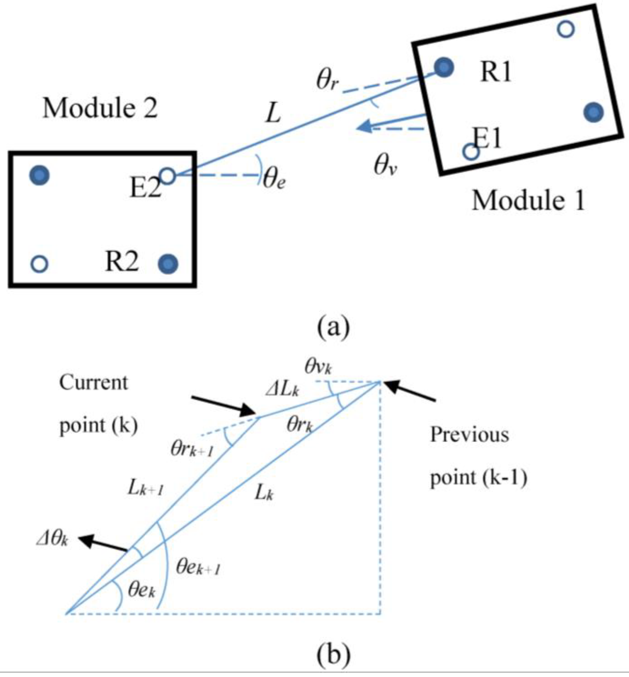
To develop an EKF, the movement of the robot is studied. After the initial alignment, Module 2 should face the rear of Module 1 with some offset and misalignment error as shown in Figure 10a. After the alignment, Module 2 is stationary and only Module 1 moves forwards and rotates for docking. Thus, the positions of emitter (E2) and receiver (R2) do not change. From Figure 10a, the relationship among the Module 1 heading direction (θv), emitter angle (θe), and receiver angle (θr) is

$$\mathrm{\theta }e=\left|\mathrm{\theta }v+\mathrm{\theta }r\right|$$

(17)

The emitter angle and receiver angle cannot be negative because the maximum IR strength is at 0°, and whether the angle increase clockwise or counter clockwise, IR strength measurement decreases That is why emitter and receiver angles should be absolute values.

From Figure 10b, when Module 2 moves forwards, current distance, L_k, with the heading angle at θv changes by ΔL_k, resulting in a new distance L_k+1. Therefore, the distances at step k + 1 can be estimated using a cosine law as follows:

$${L_{k+1}}^2={L_k}^2+\mathrm{\Delta }{L_k}^2-2\times L_k\times \mathrm{\Delta }{L}_k\times \text{cos}\mathrm{\theta }{r}_k$$

(18)

Under the assumption that θv is kept constant. For this application, θv can be assumed constant because the module heading angle change (Δθv) is small for each KF iteration step.

The distance change of Equation (19) is calculated as [19]:

$$\mathrm{\Delta }{L}_k=\frac{\mathrm{\Delta }D{R}_k+\mathrm{\Delta }D{L}_k}{2}$$

(19)

where $\mathrm{\Delta }D{R}_k$ and $\mathrm{\Delta }D{L}_k$ are the travelled distance of the right wheel and the left wheel during the time step, respectively, which are used as deterministic input, $u_k$, in Equation (12).

Figure 10. Schematics of the distances between IR sensors, and emitter and receiver angles. R1 and R2 represent receivers and E1 and E2 represent emitters. (a) Schematic of two modules and (b) relationship between receiver 1 (R1) and emitter 2 (E2) at time k.

Figure 10. Schematics of the distances between IR sensors, and emitter and receiver angles. R1 and R2 represent receivers and E1 and E2 represent emitters. (a) Schematic of two modules and (b) relationship between receiver 1 (R1) and emitter 2 (E2) at time k.

The heading angle change due to the rotation of Module 1 can be calculated as:

$$\mathrm{\theta }{v}_{k+1}=\mathrm{\theta }{v}_k+\mathrm{\Delta }\mathrm{\theta }{v}_k=\mathrm{\theta }{v}_k+\frac{\mathrm{\Delta }D{R}_k-\mathrm{\Delta }D{L}_k}{2w}$$

(20)

where w is the width of the vehicle (length between the two wheels). The orientation change ($\mathrm{\Delta }\theta v_k)$ calculation is shown in [19]. After Module 2 moves by ΔL_k, the emitter angle and the receiver angle are changed to

$$\theta e_{k+1}=\theta e_k+\mathrm{\Delta }{\theta }_k$$

(21)

$$\mathrm{\theta }{r}_{k+1}=\mathrm{\theta }{r}_k+\mathrm{\Delta }{\mathrm{\theta }}_k$$

(22)

where

$$\begin{gathered} \mathrm{\Delta }{\mathrm{\theta }}_k=\text{acos}\left(\frac{{L_k}^2+d^2-\mathrm{\Delta }{L_k}^2}{2d\times L_k}\right)=\text{acos}\left(\frac{2{L_k}^2-2L_k\mathrm{\Delta }{L}_k\text{cos}\mathrm{\theta }{r}_k}{2d\times L_k}\right) \\ =\text{acos}\left(\frac{L_k-\mathrm{\Delta }{L}_k\text{cos}\mathrm{\theta }{r}_k}{d}\right) \end{gathered}$$

(23)

Distance squared, heading angle and receiver angle are used as the state variables as:

$$x_k={[L_k^2\theta v_k\theta r_k]}^T$$

(24)

Then, the system matrix, $A_k$, can be expressed as

$$A_k={\left[\begin{array}{ccc}\frac{\partial f_{L^2}}{\partial L^2}& \frac{\partial f_{L^2}}{\partial {\mathrm{\theta }}_v}& \frac{\partial f_{L^2}}{\partial \mathrm{\theta }r}\\ \frac{\partial f_{\mathrm{\theta }v}}{\partial L^2}& \frac{\partial f_{\mathrm{\theta }v}}{\partial {\mathrm{\theta }}_v}& \frac{\partial f_{\mathrm{\theta }v}}{\partial \mathrm{\theta }r}\\ \frac{\partial f_{\mathrm{\theta }r}}{\partial L^2}& \frac{\partial f_{\mathrm{\theta }r}}{\partial {\mathrm{\theta }}_v}& \frac{\partial f_{\mathrm{\theta }r}}{\partial \mathrm{\theta }r}\end{array}\right]}_{x_k}={\left[\begin{array}{ccc}1-\frac{\mathrm{\Delta }{L}_k\times \text{cos}\mathrm{\theta }{r}_k}{L_k}& 0& 2\times L_k\times \mathrm{\Delta }{L}_k\times \text{sin}\theta r_k\\ 0& 1& 0\\ \frac{-\mathrm{\Delta }{L}_k\times \text{sin}\mathrm{\theta }{r}_k}{2L_k\times d^2}& 0& 1\end{array}\right]}_{x_k}$$

(25)

where

$$d^2={L_k}^2+\mathrm{\Delta }{L_k}^2-2\times L_k\times \mathrm{\Delta }{L}_k\times \text{cosθ}{r}_k$$

(26)

For the measurement model, $h_k\left(x_k\right)$, Equation (7) is used. In a general form, the signal strength is given by

$$S_k=\frac{a}{{L_{k+1}}^2}\times \cos (c\times \mathrm{\theta }{r}_k) \times (b-\mathrm{\theta }{e}_k)=\frac{a}{{L_{k+1}}^2}\times \cos (c\times \mathrm{\theta }{r}_k)\mathrm{ }\times (b-\left|\mathrm{\theta }{r}_k+\mathrm{\theta }{v}_k\right|)$$

(27)

Then, the linearized measurement matrix can be determined from Equation (27) as

$$\begin{gathered} C_k=[\begin{array}{cc}\frac{-a\times (b-\mathrm{abs}(\theta r_k+\theta v_k))\times \cos (c\times \theta r_k)}{{L_{k+1}}^4}& -\frac{a\times \cos (c\times \theta r_k)}{{L_{k+1}}^2}\end{array} \\ \frac{-a\times \cos (c\times \theta r_k)}{{L_{k+1}}^2}-\frac{a\times c\times (\mathrm{b}-\left|\theta r_k+\theta v_k\right|)\times \sin (c\times \theta r_k)}{{L_{k+1}}^2}] \end{gathered}$$

when $\left(\theta r_k+\theta v_k\right)>0$ and

$$C_k=[\begin{array}{cc}\frac{-a\times (b-\mathrm{abs}(\mathrm{\theta }{r}_k+\mathrm{\theta }{v}_k))\times \cos (c\times \mathrm{\theta }{r}_k)}{{L_{k+1}}^4}& -\frac{a\times \cos (c\times \mathrm{\theta }{r}_k)}{{L_{k+1}}^2}\end{array}\frac{a\times \cos (c\times \mathrm{\theta }{r}_k)}{{L_{k+1}}^2}-\frac{a\times c\times (\mathrm{b}-\left|\mathrm{\theta }{r}_k+\mathrm{\theta }{v}_k\right|)\times \sin (c\times \mathrm{\theta }{r}_k)}{{L_{k+1}}^2}]$$

(28)

when $\left(\mathrm{\theta }{r}_k+\mathrm{\theta }{v}_k\right)<0$.

3.3. Particle Filter

PF [20,21] approximates posterior using state samples, called particles, with the corresponding weights. First, the PF places a finite number of states (particles) based on the previous posterior. Then, the next state of the particle is predicted using the dynamic model. Using the predicted states and the measurements, the weight of each particle is determined as:

$$w_k^i\propto p(z_k|x_k^i)$$

(29)

where $x_k^i$ represents i^th particle of k^th iteration and $w_k^i$ represents the corresponding weight of particle $x_k^i$.

When the weights of all particles are determined, they are normalized. Then, the state is estimated based on the states and their corresponding weights as:

$$x_k={\displaystyle \sum }{w}_k^i\times x_k^i$$

(30)

Then, new particles are resampled based on the weights and the covariance of the system noise.

To achieve high accuracy, the number of particles should be large enough to represent the posterior distribution. Although PF does not require calculating error covariance, Kalman gain, and inverse of matrices, it requires higher computational power than an EKF due to the requirement of a large number of particles for accurate state estimation.

For the proposed PF, the same states as EKF are used as shown in Equation (24). For the initial state distribution, the receiver angle and heading angle of the particles are spread evenly, and the distance of each particle is calculated based on measurement, receiver angle and heading angle using Equation (7).

For the prediction model, Equations (18), (20) and (22) are used, and for the measurement model, Equation (27) is used.

4. Simulation and Experiments

In this section, we provide simulation and experimental results to validate the performance of developed estimators. In addition, in the experiments, we demonstrate the docking performance for two mobile modules and repeat the experiments several times to prove its robustness as well.

4.1. Simulations

Both EKF and PF were simulated to determine which state estimator offers a better solution for this application. For the simulations of PF, the initial heading angle and receiver is spread from −0.05 radian to 0.05 radian (2.9°). Our PF uses 121 particles, because after several simulations we found out increasing the number of particles beyond 121 will not improve the results considerably and instead will add to the computational cost. Therefore, for the PF we keep the number of particles to be 121, which is optimum, both in terms of accuracy and computational cost.

Two different case studies are considered and the results of EKF and PF were compared. These two case studies are: 1) when the initial estimations are accurate, and 2) when initial estimations are not accurate.

It was assumed that the encoders have standard deviation errors of 10% due to slippage of the robot tires, and the IR sensor has a standard deviation error of 4% of the IR signal strength.

4.1.1. Using Correct Initial Position and Orientations

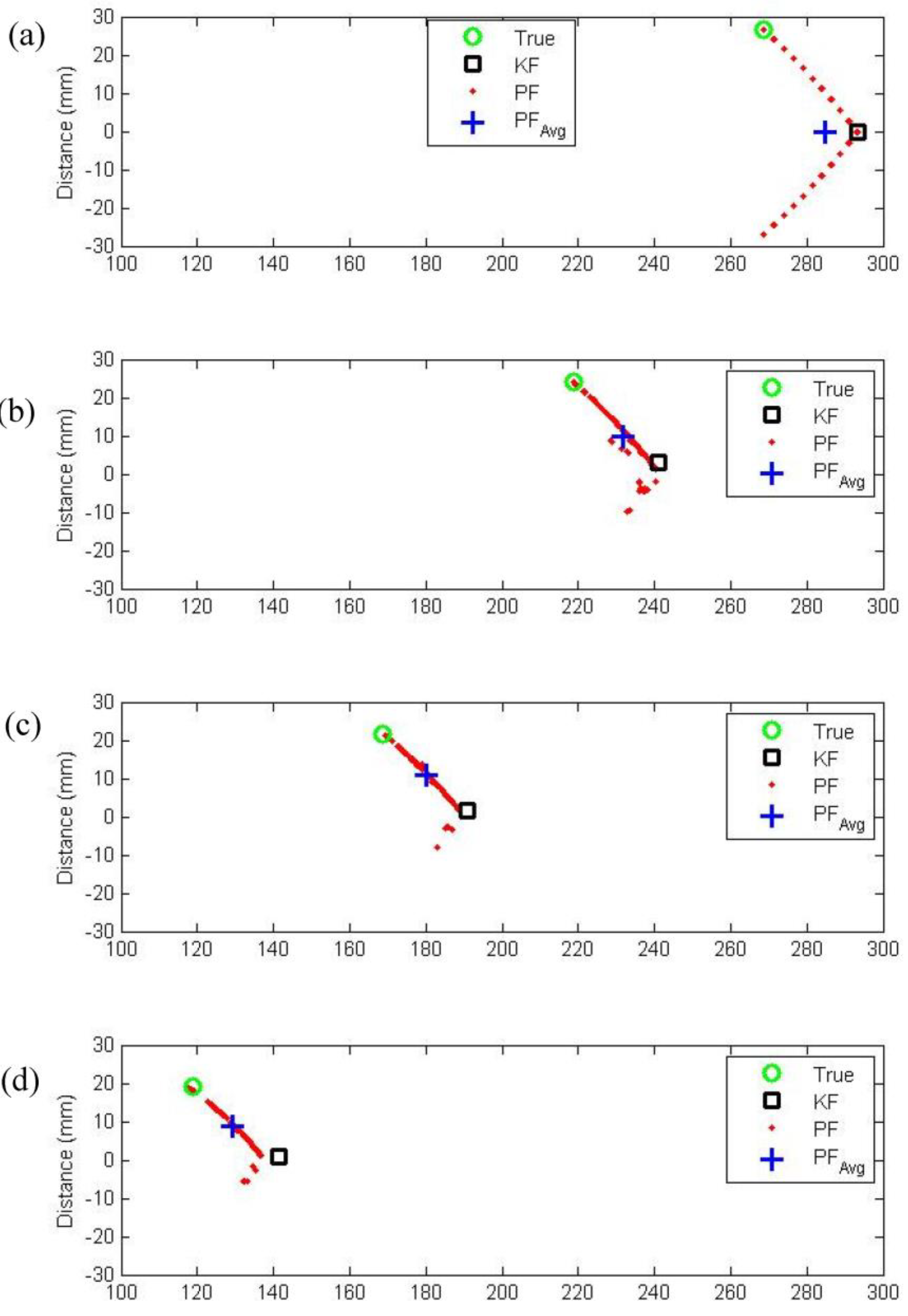
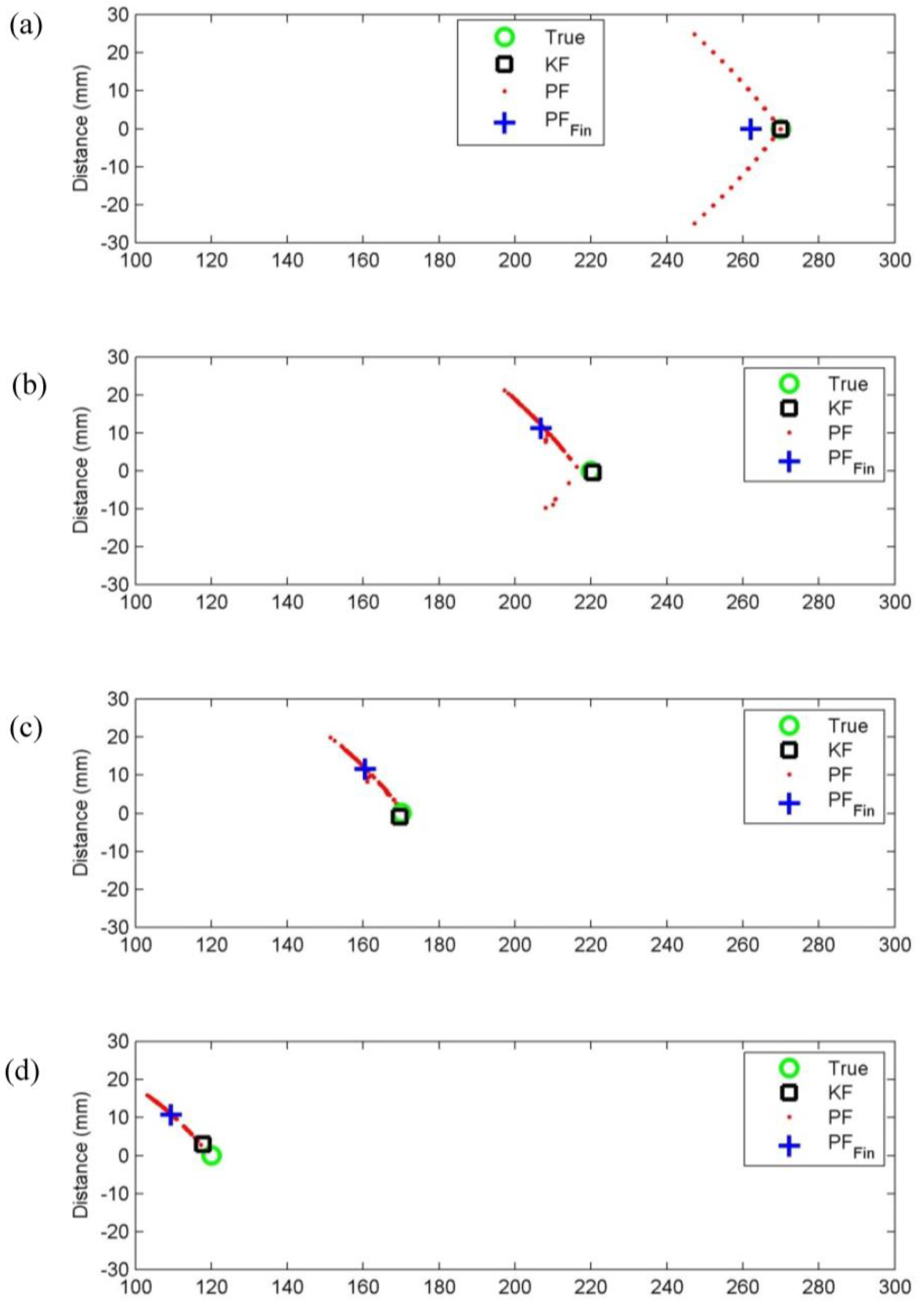
The initial position and orientations of the two modules are accurately estimated for the first simulation. The emitter and the receiver are 270 mm apart, and the two modules are perfectly aligned, meaning both heading angle and receiver angle are 0°. The positions of Module 1 at different time steps of simulation are shown in Figure 11. The green circle represents true position of the Module 1, the black rectangle represents position estimation using the EKF, red “x” marks represents particles of the PF, and “+” represents the final states which is the average of the PF states.

Figure 11. Position comparison of truth, EKF, and PF when the initial estimation is accurate. (a) initial position, (b) after moving 50 mm, (c) after moving 100 mm, and (d) after moving 150 mm, which represents docking position

Figure 11. Position comparison of truth, EKF, and PF when the initial estimation is accurate. (a) initial position, (b) after moving 50 mm, (c) after moving 100 mm, and (d) after moving 150 mm, which represents docking position

Figure 11a shows that the EKF position matches the true position because the initial estimation is known. The particles of PF are spread evenly from 0° as well. Figure 11b shows the states after Module 1 moves 50 mm forward. It shows that particles are more condensed than Figure 11a because all the particles with high errors are eliminated. The EKF position estimation has some error compared to the true value. As iteration continues, particles get closer to the true value. On the other hand, the EKF error tends to increase as time proceeds, but shows better accuracy than PF. The state estimations of this simulation are shown in Table 1. The table shows that estimations of EKF are more accurate than PF.

Table 1. Position comparison when initial estimation of EKF is correct.

	Position (mm)	Heading Angle (°)	Receiver Angle (°)
True	120.4	0	0
EKF	117.8	0.83	0.66
PF	110.0	1.78	3.89

Table 1. Position comparison when initial estimation of EKF is correct.

	Position (mm)	Heading Angle (°)	Receiver Angle (°)
True	120.4	0	0
EKF	117.8	0.83	0.66
PF	110.0	1.78	3.89

In order to quantify the error more accurately, the simulation is repeated 200 times and the average error of EKF and PF are evaluated (Table 2). Table 2 demonstrates that the EKF has much lower error than the PF for this application.

Table 2. Average state estimation error with 200 simulations.

	Position (mm)	Position δ	Heading angle (°)	Heading δ	Emitter angle (°)	Emitter δ
EKF	2.2	1.7	1.10	1.40	0.57	0.74
PF	8.7	5.0	1.03	0.93	4.32	2.82

Table 2. Average state estimation error with 200 simulations.

	Position (mm)	Position δ	Heading angle (°)	Heading δ	Emitter angle (°)	Emitter δ
EKF	2.2	1.7	1.10	1.40	0.57	0.74
PF	8.7	5.0	1.03	0.93	4.32	2.82

4.1.2. Using Incorrect Initial Position and Orientations

The simulation was repeated with the same condition as previous simulation but the true heading angle of Module 1 is set to 0.05 radian (2.86°) and emitter angle is set to 0.05 radian. The simulation results are shown in Figure 12. Figure 12a shows that the EKF position does not match the true position due to the initial estimation error. Since it was assumed that the two modules are aligned, Figure 12a shows that the initial states of EKF is far behind the true position. Although the iteration continues, EKF position estimation does not converge to the correct position due to the incorrect initial estimation. On the other hand, PF converges to the true estimation as the iteration continues.

Table 3 shows the comparison between PF, EKF, and true state estimations after two modules are docked. Table 3 shows that the PF estimation converges to the correct states, but EKF estimation does not.

The simulations were repeated 200 times to study the average error of EKF and PF as shown in Table 4. Estimation errors of PF of two different simulations (Table 2 and Table 4) are not significantly different. However, the state estimation error of EKF increased significantly when the initial estimation error is not accurate.

The simulations show that EKF is more accurate when the initial estimation is known, but when the initial estimation is not accurately estimated, EKF does not converge to the correct value. However, PF converges to the correct state because the fittest particles survive. It should be noted that the EKF iteration was 130 times faster than the PF iteration with 121 particles in this simulation. Also, even though it is not shown on this simulation, the estimation error of PF increases if the initial error is far away from the initial samples of PF (i.e., receiver angle = 0.15 rad). Thus, EKF is considered as a better solution if the initial state is correctly estimated especially for an application that uses autonomous robots with limited on-board CPU computational power.

Figure 12. Position comparison of truth, EKF, and PF when the initial estimation is not correct. (a) initial position, (b) after moving 50 mm, (c) after moving 100 mm, and (d) after moving 150 mm, which represents docking position

Figure 12. Position comparison of truth, EKF, and PF when the initial estimation is not correct. (a) initial position, (b) after moving 50 mm, (c) after moving 100 mm, and (d) after moving 150 mm, which represents docking position

Table 3. Position comparison when initial estimation of EKF is not correct.

	Position (mm)	Heading Angle (°)	Receiver Angle (°)
True	120.4	2.86	6.43
EKF	141.5	0.42	0.01
PF	129.7	0.85	3.18

Table 3. Position comparison when initial estimation of EKF is not correct.

	Position (mm)	Heading Angle (°)	Receiver Angle (°)
True	120.4	2.86	6.43
EKF	141.5	0.42	0.01
PF	129.7	0.85	3.18

Table 4. Average state estimation error with 200 simulations.

	Position (mm)	Position δ	Heading angle (°)	Heading δ	Emitter angle (°)	Emitter δ
EKF	23.1	3.0	4.50	1.57	6.22	0.39
PF	9.9	5.4	3.16	1.09	2.62	2.40

Table 4. Average state estimation error with 200 simulations.

	Position (mm)	Position δ	Heading angle (°)	Heading δ	Emitter angle (°)	Emitter δ
EKF	23.1	3.0	4.50	1.57	6.22	0.39
PF	9.9	5.4	3.16	1.09	2.62	2.40

4.2. Experiments

Two modules were built and docking experiments were conducted to test the robot’s docking ability and the accuracy of the proposed EKF. In order to quantify the accuracy of the EKF, the true positions of each module and connector are measured using an ultrasonic position sensor (CMS10, Zebris) whose positional error is typically less than 2 mm. Two ultrasonic emitters are attached to the body of the module to find the orientation of the module and one ultrasonic emitter is attached to the connector.

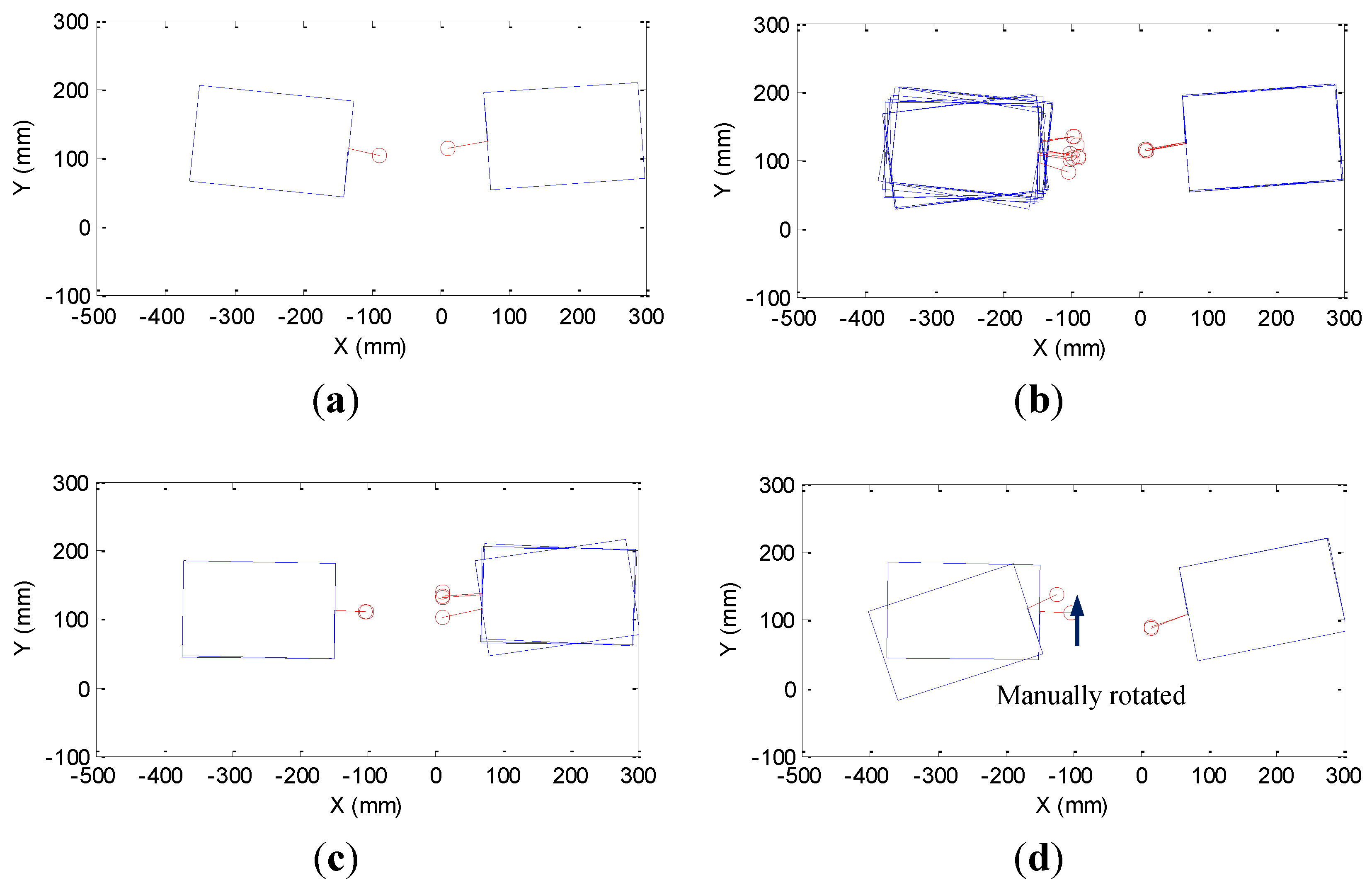
Three different docking experiments were conducted. In the first case, two modules are initially facing each other. For the second case, the modules are initially misaligned by 90°. Finally, in the third case, orientation error is introduced by manually rotating one module before the EKF is applied.

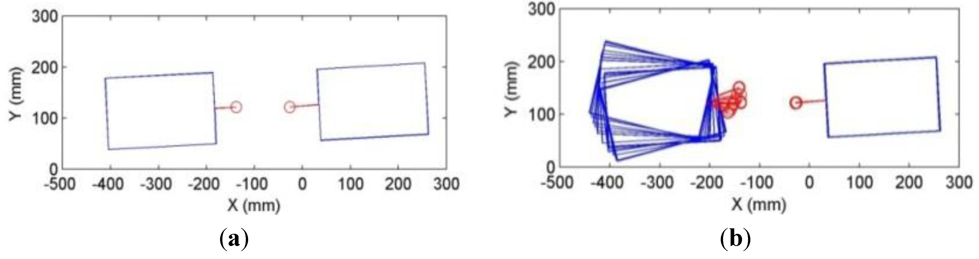
Modules Facing Each Other

The two modules are initially orientated so that they are facing each other, and then the docking process is performed. Figure 13 shows the experiment progression. Red circles represent the ultrasonic sensor attached to the connector and each blue box represents the module obtained from two ultrasonic sensors. Initially, the two modules are facing each other as shown in Figure 13a. When docking is initiated, Module 1 rotates to align with Module 2 (Figure 13b). After Module 1 is aligned, Module 2 is aligned (Figure 13c). Once both modules are aligned, Module 1 moves forward until the distance estimation from EKF becomes 120 mm (Figure 13d), which is the length of the two connectors. While Module 1 moves forward, the EKF is activated to estimate the distance between the two modules. When the estimated distance is less than 120 mm, Module 1 moves backwards to check if the modules are docked. If docking is successful, Module 1 will drag Module 2, and the distance between the two modules remains 120 mm. In this case, IR receiver will measure high signal strength. Otherwise, only Module 1 moves backward, and the IR signal strength measurements will be low. Figure 13e shows that Module 1 moves backwards with Module 2 because docking was successful. Therefore, the IR signal strength is high, and the system concludes that the two modules are successfully docked, and the modules stop (Figure 13f). A video of experiments can be found in the supplementary file.

Figure 13. Experimental results when two modules are initially facing each other. (a) initial state, (b) Alignment of Module 1, (c) Alignment of Module 2, (d) Module 1 moves forwards for docking, (e) Module 1 moves backwards for checking successful docking, and (f) Docking process completed.

Figure 13. Experimental results when two modules are initially facing each other. (a) initial state, (b) Alignment of Module 1, (c) Alignment of Module 2, (d) Module 1 moves forwards for docking, (e) Module 1 moves backwards for checking successful docking, and (f) Docking process completed.

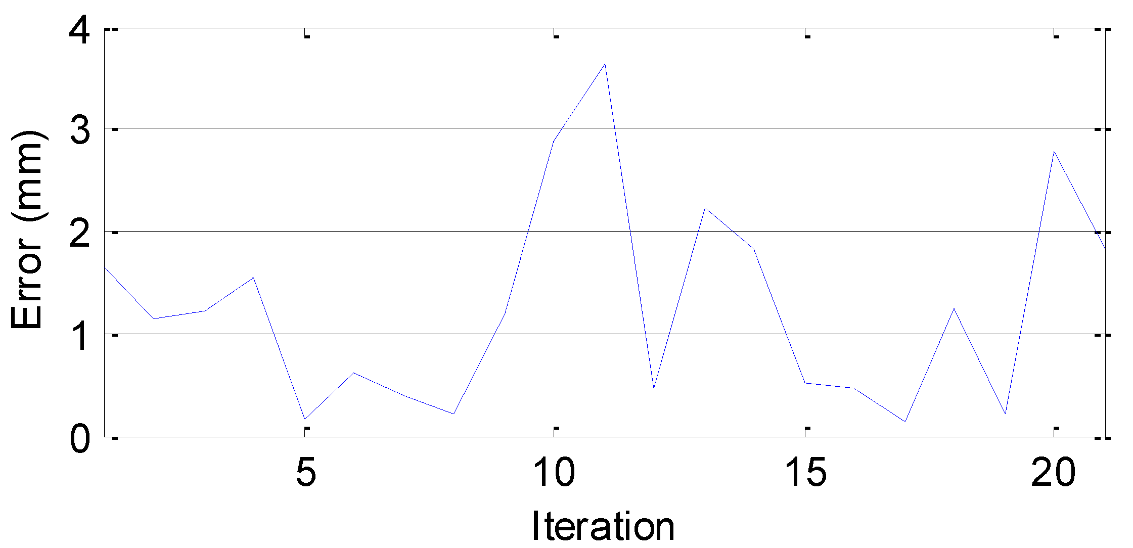
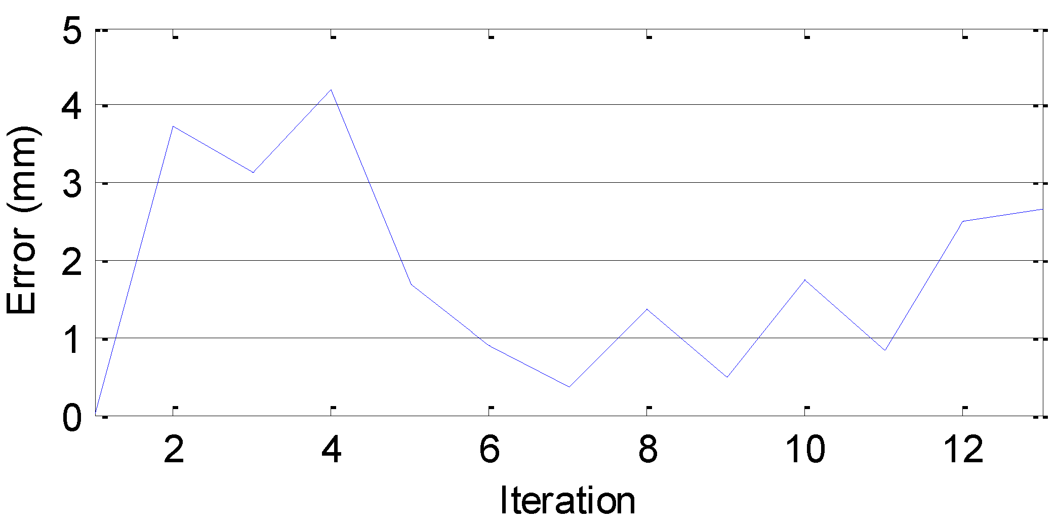
The EKF is activated when Module 1 starts moving towards Module 2 (Figure 13d) and is deactivated when the distance, L, is less than 120 mm. The distance estimation error of EKF is shown in Figure 14. The error graph shows that the distance estimation error is less than 4 mm while Module 1 is moving forward for docking. The magnitude of the distance error is within the tolerance of the magnetic connector.

Figure 14. EKF distance error of when two modules are facing each other.

Figure 14. EKF distance error of when two modules are facing each other.

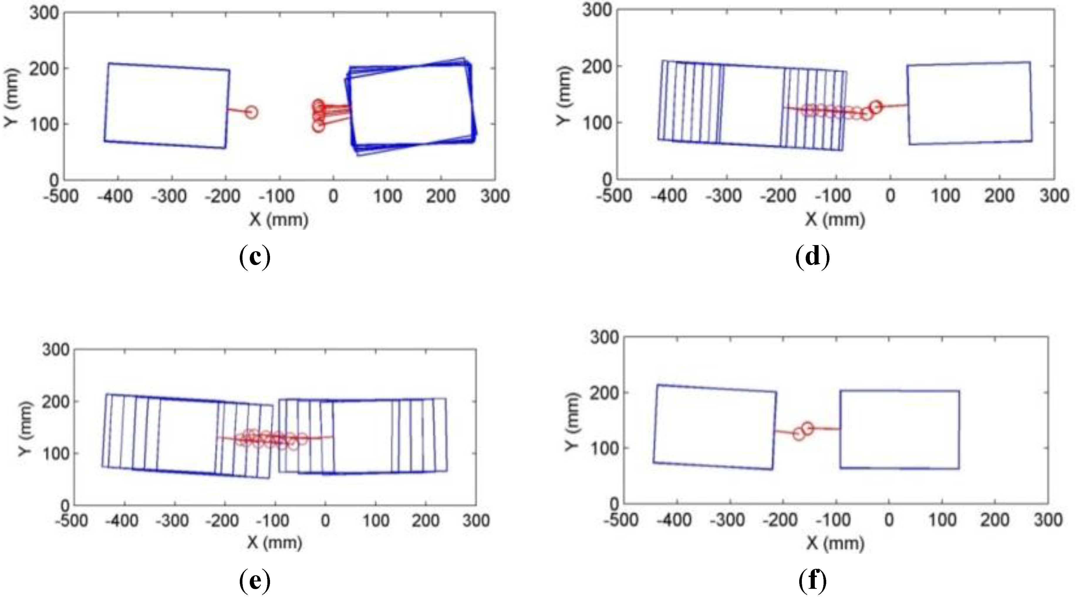
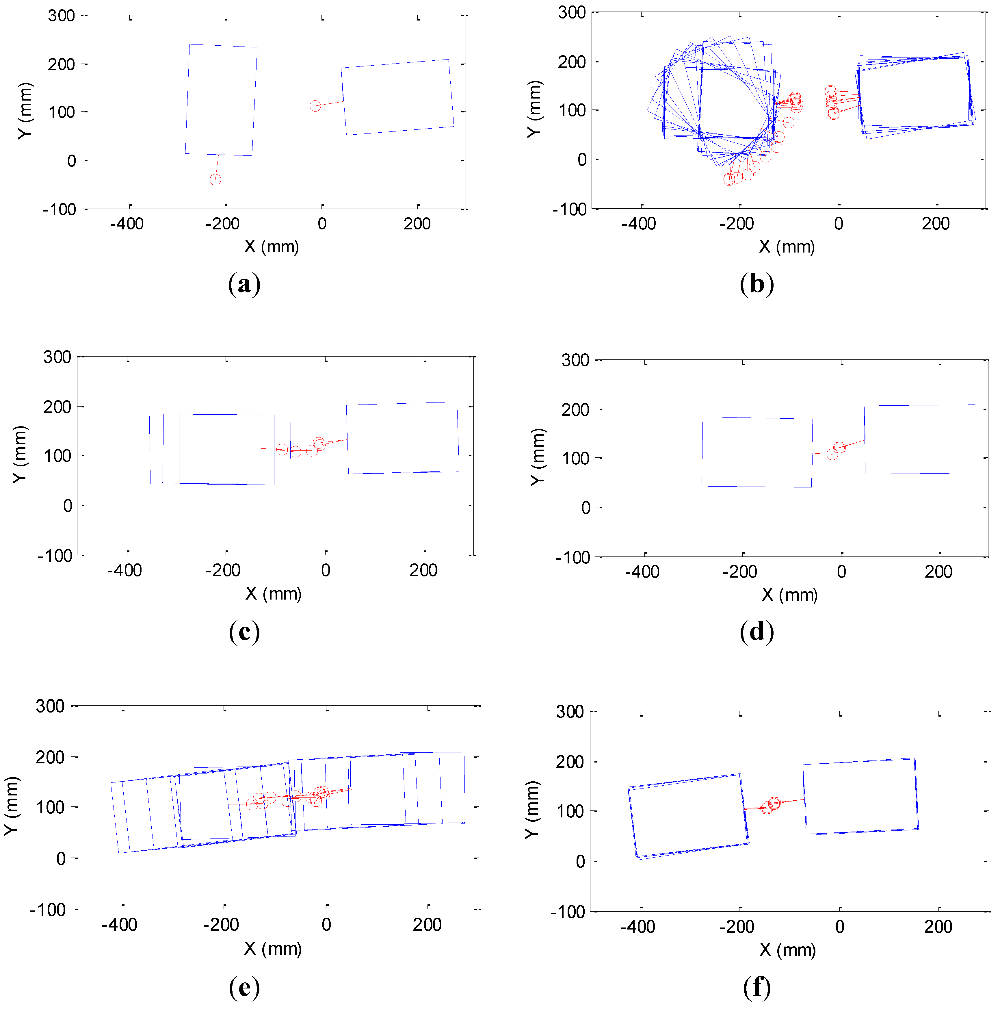
4.3. Docking Modules at 90° Angle

Initially, Module 1 faces Module 2 with an angle of 90° as shown in Figure 15a. First, Module 1 keeps rotating until it roughly aligns with Module 2. Then, Module 1 rotates for the fine-alignments (Figure 15b). Next, Module 2 is aligned. After the alignments, Module 1 moves forward for docking (Figure 15c). However, Figure 15c shows offset between two modules, which means there is some error in emitter angle (θe) and receiver angle (θr). This also results in distance error. Therefore, even when Module 1 docks with Module 2 successfully as shown in Figure 15c, it keeps moving forward and pushes the connector of Module 2. Thus, the connector of Module 2 is tilted a bit further in Figure 15d compared to Figure 15c. When distance estimation is 120 mm, Module 1 moves back to check if docking is successful (Figure 15e). Since docking is completed successfully, Module 1 stops (Figure 15f). This experiment shows that magnets pull each other and successfully dock even with a small offset error because the universal joint and suction cup (Figure 2) make the magnets move freely. The error analysis in Figure 16 shows that the error is similar as the previous case.

Figure 15. Experimental results when two modules are misaligned roughly 90°. (a) Initial state, (b) Alignment of Module 1and Module 2, (c) Module 1 moves forwards for docking, (d) Tow modules dock, (e) Module 1 moves backwards for checking successful docking, and (f) Docking process completed.

Figure 15. Experimental results when two modules are misaligned roughly 90°. (a) Initial state, (b) Alignment of Module 1and Module 2, (c) Module 1 moves forwards for docking, (d) Tow modules dock, (e) Module 1 moves backwards for checking successful docking, and (f) Docking process completed.

Figure 16. EKF distance error when misalignment is 90°.

Figure 16. EKF distance error when misalignment is 90°.

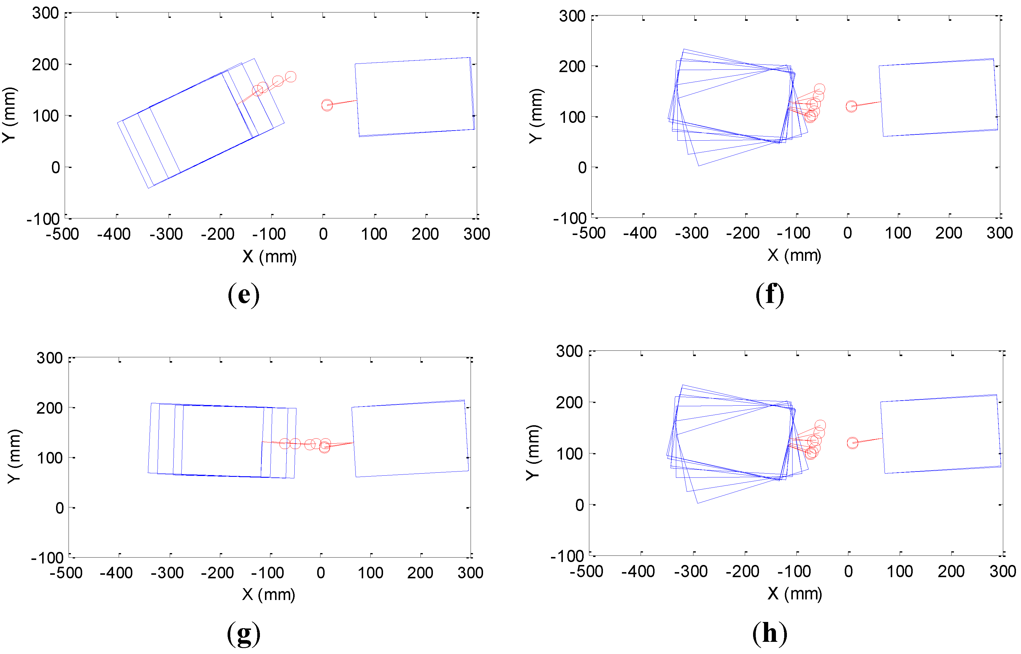
Incorrect Initial State Estimation

The performance of the docking algorithm is evaluated in the presence of the initial state estimation errors. For this experiment, Module 1 is lifted up and manually rotated before EKF is applied. Therefore, errors are introduced to the initial state estimations. Figure 17 shows the progress of this experiment. The initial states of the two modules are shown in Figure 17a. First, Module 1 is aligned (Figure 17b) and then Module 2 is rotated to be aligned (Figure 17c). Before Module 2 is completely aligned, Module 1 is manually rotated to introduce errors. 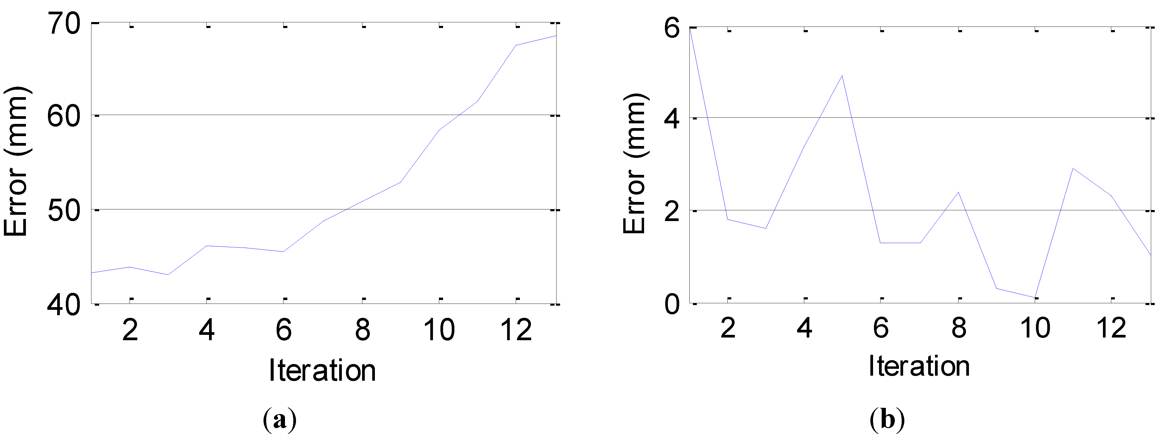Figure 17d shows that Module 1 was initially aligned with Module 2, but manually rotated. Then, Module 1 moves forward as shown in Figure 17e. The distance estimation error during this step is shown in Figure 18a. The figure shows that the initial distance error is greater than 40 mm due to incorrect initial estimation.

Figure 17. Experimental results: Module 1 is manually rotated just before KF is initialized so that initial estimations of distance and emitter and receiver angles are incorrect. (a) Initial state, (b) Alignment of Module 1, (c) Alignment of Module 2, (d) Module 1 was rotated manually to introduce orientation error, (e) Module 1 moves forwards for docking, (f) Module 1 rotates again for realignment, (g) Module 1 moves forwards for docking, and (h) Module 1 moves backwards for checking successful docking.

Figure 17. Experimental results: Module 1 is manually rotated just before KF is initialized so that initial estimations of distance and emitter and receiver angles are incorrect. (a) Initial state, (b) Alignment of Module 1, (c) Alignment of Module 2, (d) Module 1 was rotated manually to introduce orientation error, (e) Module 1 moves forwards for docking, (f) Module 1 rotates again for realignment, (g) Module 1 moves forwards for docking, and (h) Module 1 moves backwards for checking successful docking.

Figure 18. EKF distance error with incorrect initial state estimation (a) before re-initialization (b) after re-initialization.

Figure 18. EKF distance error with incorrect initial state estimation (a) before re-initialization (b) after re-initialization.

Also, as Module 1 moves forwards, the distance error keeps increasing. Figure 17f shows that Module 1 stops and rotates for realignment because the algorithm identified that initial estimations were not correct. After Module 1 is realigned, EKF is initialized again and Module 1 moves forward for docking, as shown in Figure 17g.

Figure 17g is shown in Figure 18b. The error graph shows that the distance error after realignment is reduced to the level of previous two scenarios. Figure 17h shows that Module 1 drags Module 2 to check for successful docking. This experiment shows that the proposed algorithm is robust enough to dock two modules even if high initial estimation error exists.

4.4. Repeatability

To prove the repeatability of the experimental results, the above three experiments were repeated five times each and the average distance errors at docking were found. These results have been tabulated in Table 5. Table 5 shows that the errors are small in all three cases, and the error difference of the three cases is insignificant. The results demonstrate that the EKF accurately estimates the distance between the two robots in all three cases with a small error.

Table 5. Average state estimation distance error of three different scenarios.

	Facing Each Other	90° Misalignment	With Error
Distance error (mm)	2.11	1.53	1.89

Table 5. Average state estimation distance error of three different scenarios.

	Facing Each Other	90° Misalignment	With Error
Distance error (mm)	2.11	1.53	1.89

5. Conclusions

This paper presents a novel docking system for modular mobile self-reconfigurable robots using low cost sensors. Low cost IR sensors and encoders are utilized to estimate the distance and the orientation of the modules. The signal strength of the IR sensor was modeled using emitter and receiver angles as well as the distance. Based on the IR sensor and motion models, an EKF and a PF were developed to estimate the distance and orientation more accurately. Both state estimators were simulated to compare their performance in this application.

Simulation results showed that EKF yields higher accuracy when the initial state is correctly estimated, but PF results in a better accuracy when the initial estimation is not correct. Since the EKF is accurate when the initial estimation is correct and is much faster than PF, EKF was considered a better estimator for this application, which uses autonomous robots with limited CPU power. To make the EKF work even with high initial state estimation error, an efficient docking algorithm was developed. The proposed docking algorithm can estimate the initial state, detect if docking is completed, and detect if the EKF state estimation is incorrect. In case the initial estimation is not correct, the algorithm detects the error and aligns the module again. If docking is not successful, the algorithm re-initiates to achieve successful docking.

The proposed system with the EKF was experimentally tested in three different case studies. When the initial estimation is correctly identified, the EKF can correctly estimate the position, which allows successful docking. When the initial state is not correctly estimated, the distance estimation diverges from the true values. However, the proposed algorithm can identify the error, and make the modules re-align. After the re-alignment, the distance estimation of EKF is accurate and docking can be successfully completed. These experiments demonstrate the robustness of the proposed docking system.

The experimental results demonstrate that the proposed system can accurately estimate the distance between the two modules, and make the robots dock successfully even when the initial distance between robots is not calculated correctly. Therefore, our contribution of this work lies in the development of a robust, cost-effective, and reliable docking mechanism with accurate distance estimations.

IR sensors present a challenge for long range docking system because the signal strength decreases quadratically over distance. IR sensors can be used for a long range, but they require high power consumption. Thus, for long-range applications, another sensing system such as RF can be exploited to steer the modules closer to each other and then IR sensing system can be used for docking when the modules are in close proximity.