
Vision-Based Cooperative Pose Estimation for Localization in Multi-Robot Systems Equipped with RGB-D Cameras

Abstract
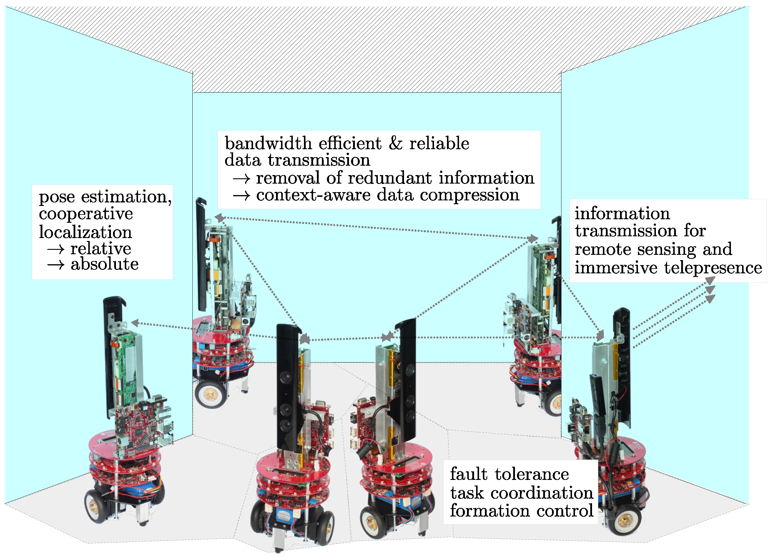
:1. Introduction
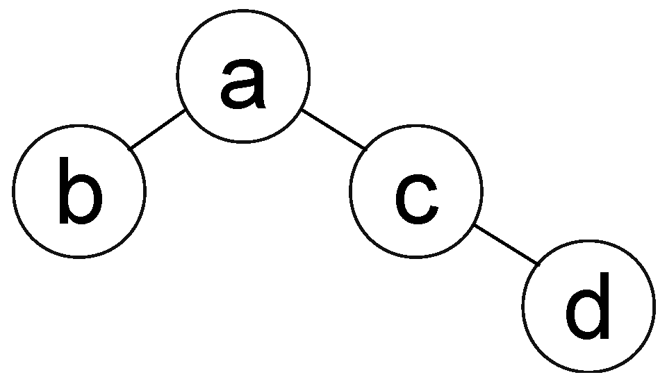
- Construction of a robot dependency graph based on the overlapping ratio between neighboring robots.
- Development of a procedure to determine the relative pose of multiple RGB-D camera equipped robots.
- By contrast to the conventional approaches that only utilize color information, our approach takes the advantages of the combination of RGB and depth information.
- The locations and orientations of robots are determined up to the real world scale directly without involving scale ambiguity problem.
- Extensive experiments using synthetic and real world data were conducted to evaluate the performance of our algorithms in various environments.
2. A Multi-Robot System Using RGB-D Cameras As Visual Sensors
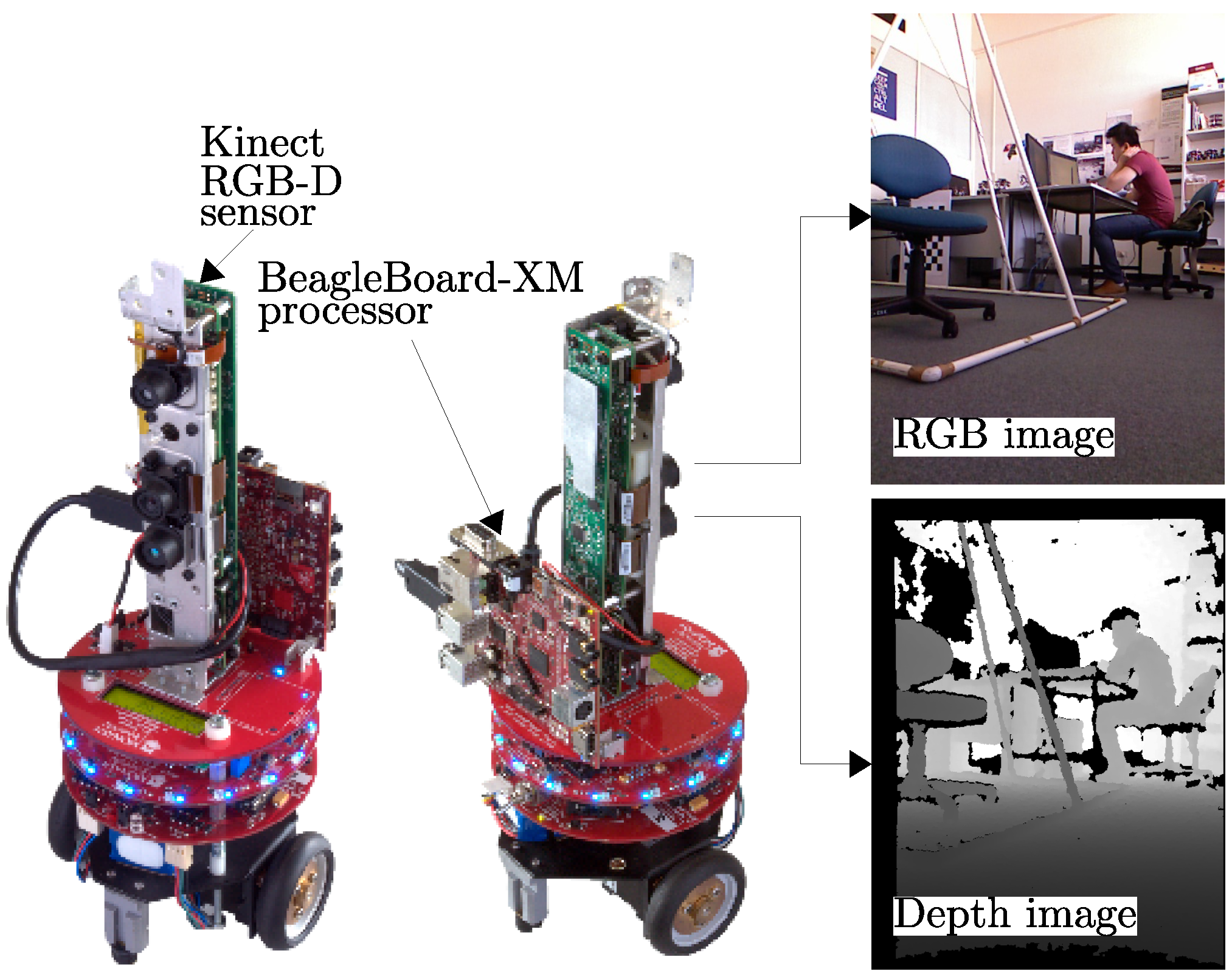
2.1. eyeBug: A Robot Equipped with RGB-D Camera

2.2. Characteristics of RGB-D Camera
3. Self-Calibration Cooperative Pose Estimation
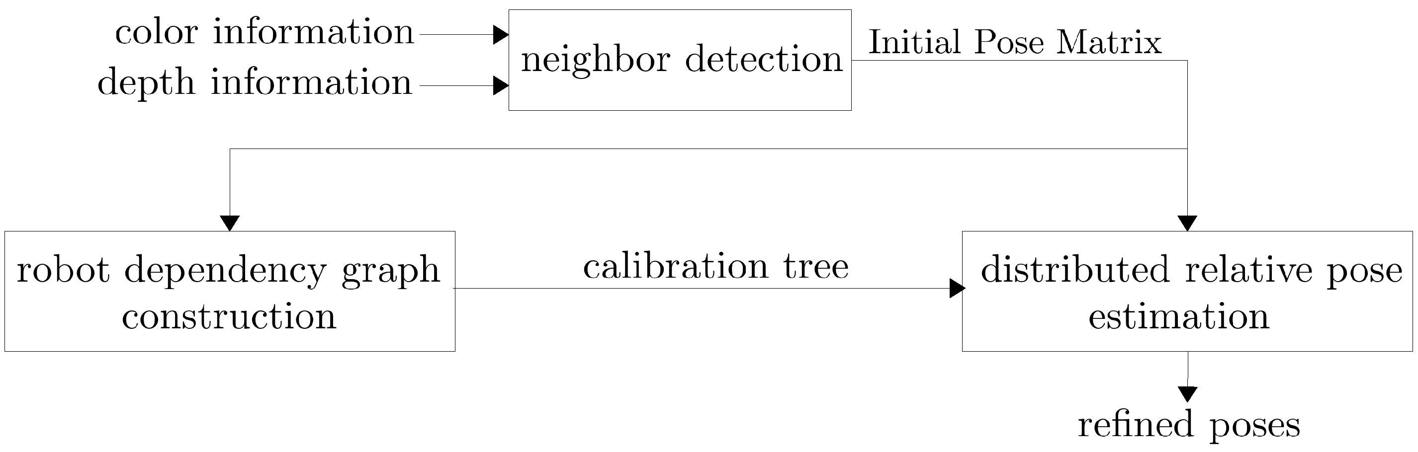
3.1. Overview

| Notation | Description |
|---|---|
| Depth image captured by robot a. | |
| Vector representing a real world point in Euclidean space. | |
| Principal point coordinates of the pinhole camera model. | |
| Focal length of the camera in horizontal and vertical axes. | |
| Transformation matrix describing the relative pose between robots a and b. | |
| Sampled points on the depth image captured by robot a. | |
| Corresponding points of on the depth image captured by robot b. | |
| Number of sampled points on . | |
| Set of sample points on . | |
| Set of corresponding points of on . | |
| Surface normal at point . | |
| Weight parameter for correspondence established between and . | |
| Update transformation matrix in each iteration. | |
| An element of a 6D motion vector. | |
| 6D motion generator matrices. |
3.2. Assumptions
- Intrinsic parameters of the RGB-D camera on each robot are calibrated prior to deployment,
- At least two robots in the system have overlapping FoVs;
- The scene is static and the robots do not move during the localization process, and
- The robots can form an ad-hoc network and directly communicate with each other.
3.3. Neighbor Detection and Initial Relative Pose Estimation
| No. | 1 | 2 | 3 | 4 | No. | 1 | 2 | 3 | 4 |
| 1 | × | 1 | × | w12 | w13 | w14 | |||
| 2 | × | 2 | w21 | × | w23 | w24 | |||
| 3 | × | 3 | w31 | w32 | × | w34 | |||
| 4 | × | 4 | w41 | w42 | w43 | × |
3.4. Selection of Relative Pose
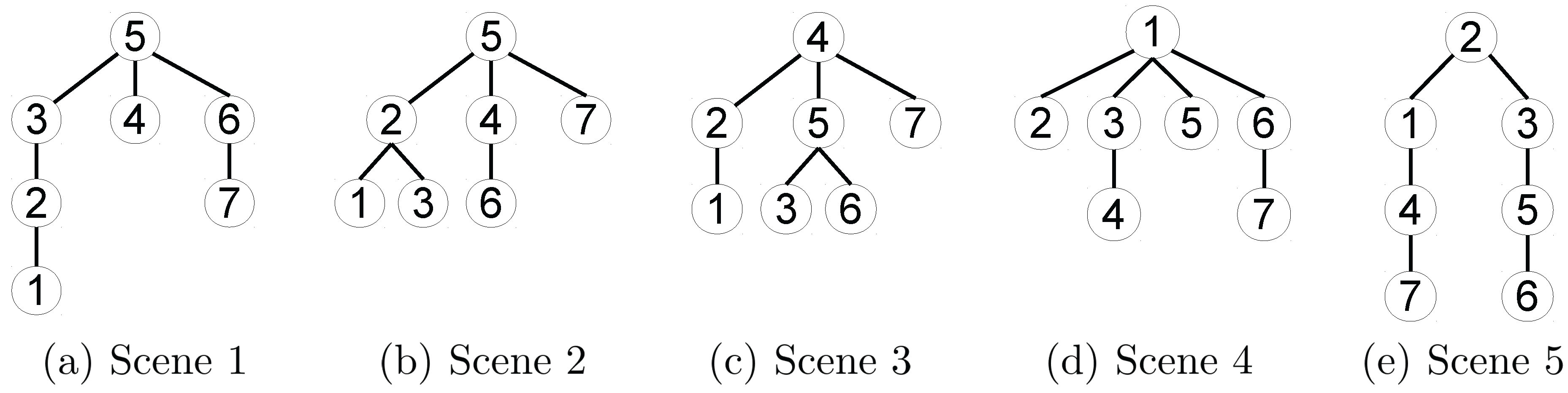
3.4.1. Robot Dependency Graph Construction
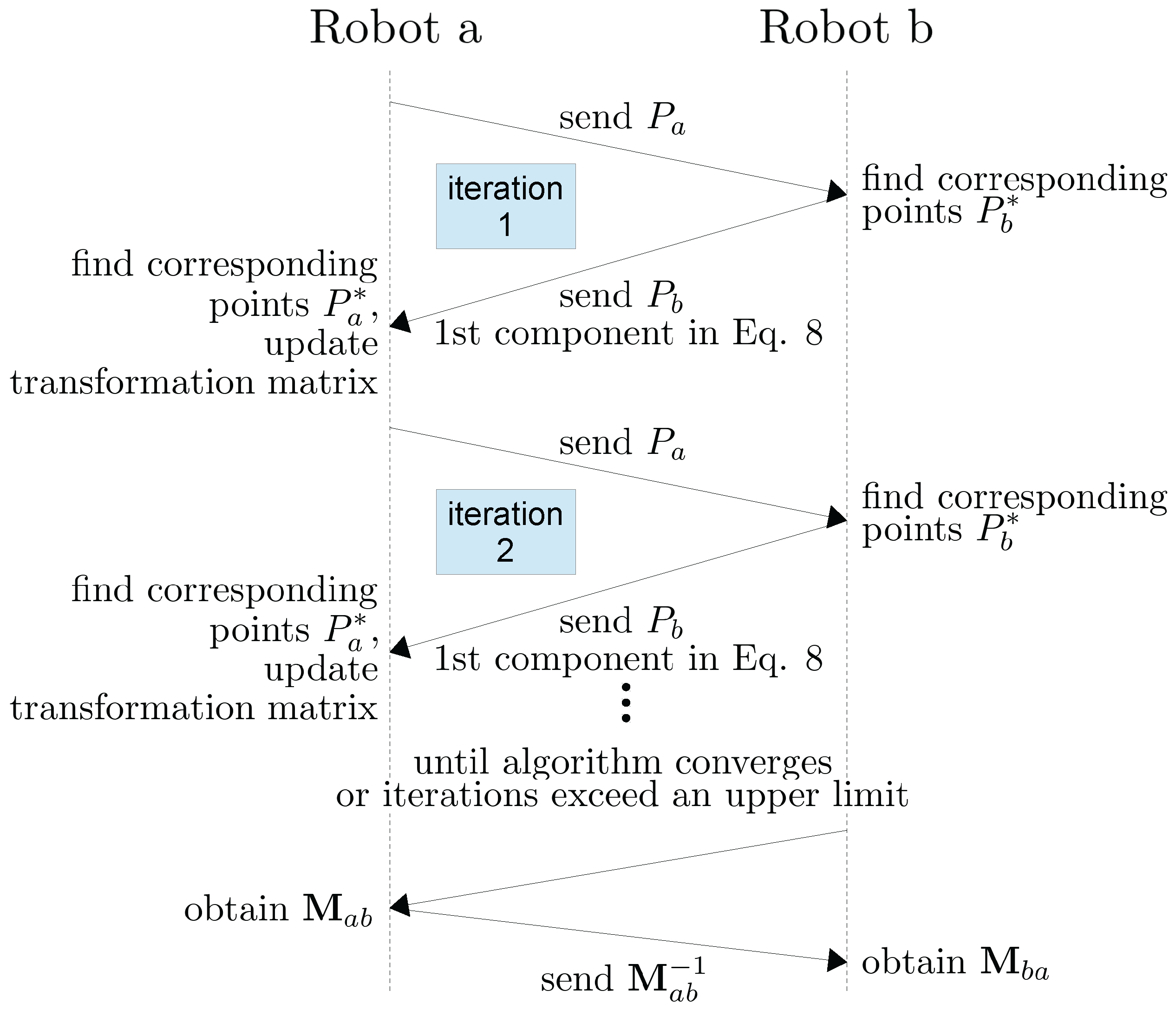
3.5. Distributed Relative Pose Estimation Algorithm
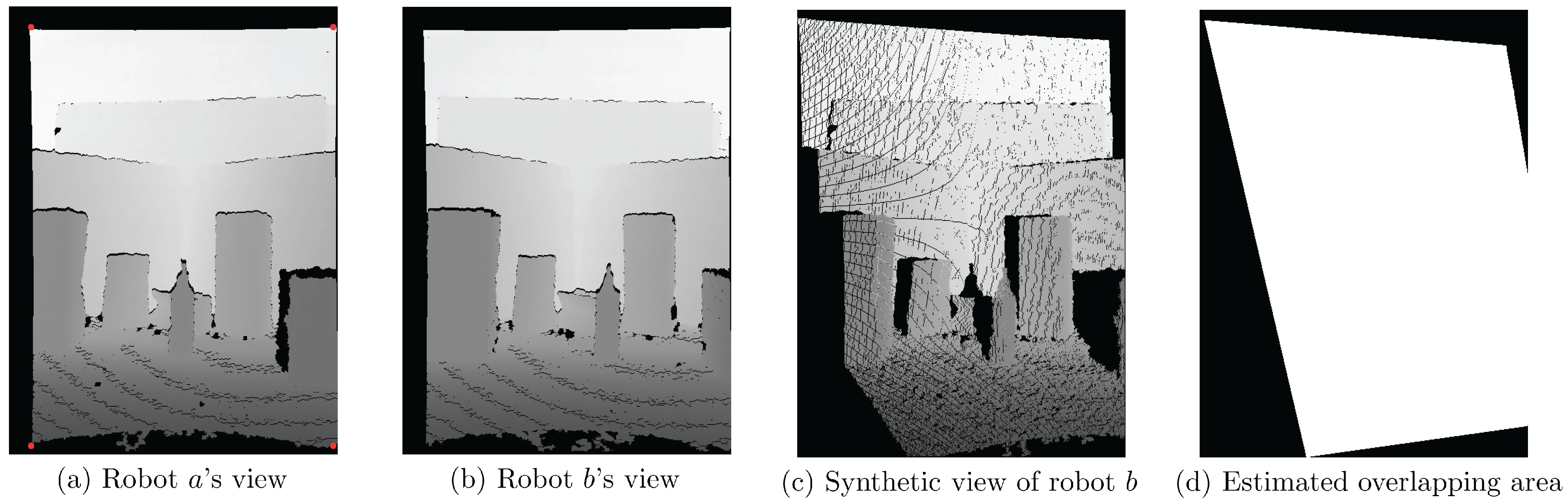
- the sum of squared distances in the forward direction from depth images to , and
- the sum of square distances in the backward direction from to .
| Algorithm 1 Relative pose refinement procedure | |
| 1: | Capture a depth image, Za, on robot a, and capture a depth image, Zb, on robot b. |
| 2: | Initialize the transformation matrix, Mab, by the initial relative pose. |
| 3: | procedure REPEAT UNTIL CONVERGENCE |
| 4: | Update depth frame Za according to transformation matrix. |
| 5: | Randomly sample points from to form set , |
| , | |
| 6: | Randomly sample points from to form set , |
| . | |
| 7: | Find the corresponding point set, , of in , |
| ; | |
| Find the corresponding point set, , of in , | |
| . | |
| ⊳ The correspondences are established using the project and walk method with a neighborhood size of 3x3 based on the nearest neighbor criteria | |
| 8: | Apply the weight function bidirectionally, |
| , | |
| 9: | Compute and update transformation matrix based on current bidirectionally weighted correspondences |
| 10: | end procedure |

4. Experimental Results and Discussion
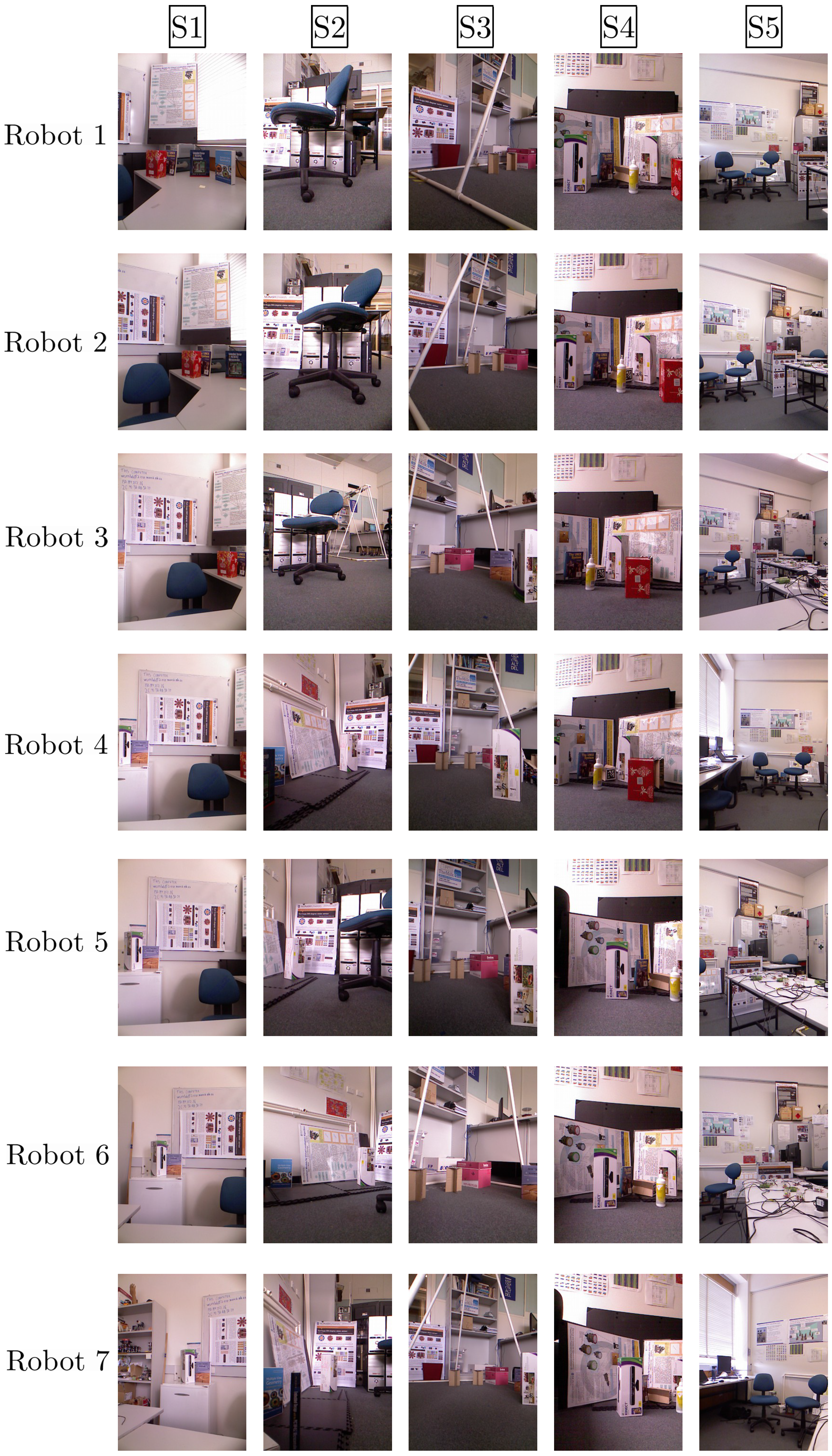
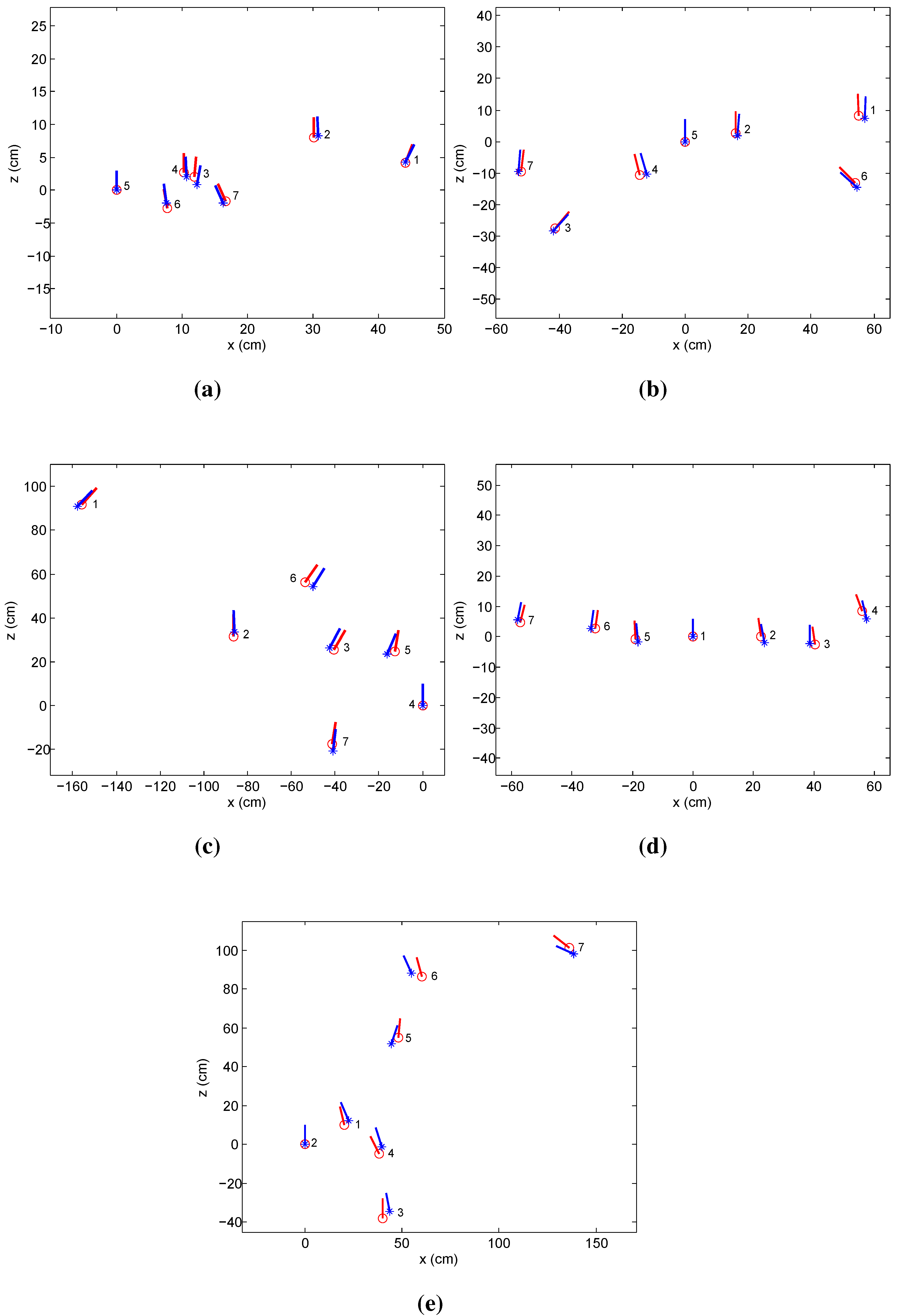
4.1. Indoor Experiments


| Data Set | Sensing Range | Average Absolute Error | Localization Average Relative Error | ||
|---|---|---|---|---|---|
| Max (m) | Average (m) | Location (mm) | Orientation (∘) | ||
| 1 | 1.92 | 1.47 | 10.0 | 1.6 | 2.26% |
| 2 | 6.23 | 1.72 | 14.8 | 2.3 | 1.36% |
| 3 | 3.95 | 1.86 | 25.1 | 2.7 | 1.39% |
| 4 | 1.79 | 1.41 | 12.6 | 2.1 | 1.12% |
| 5 | 6.02 | 4.14 | 64.7 | 6.2 | 3.81% |
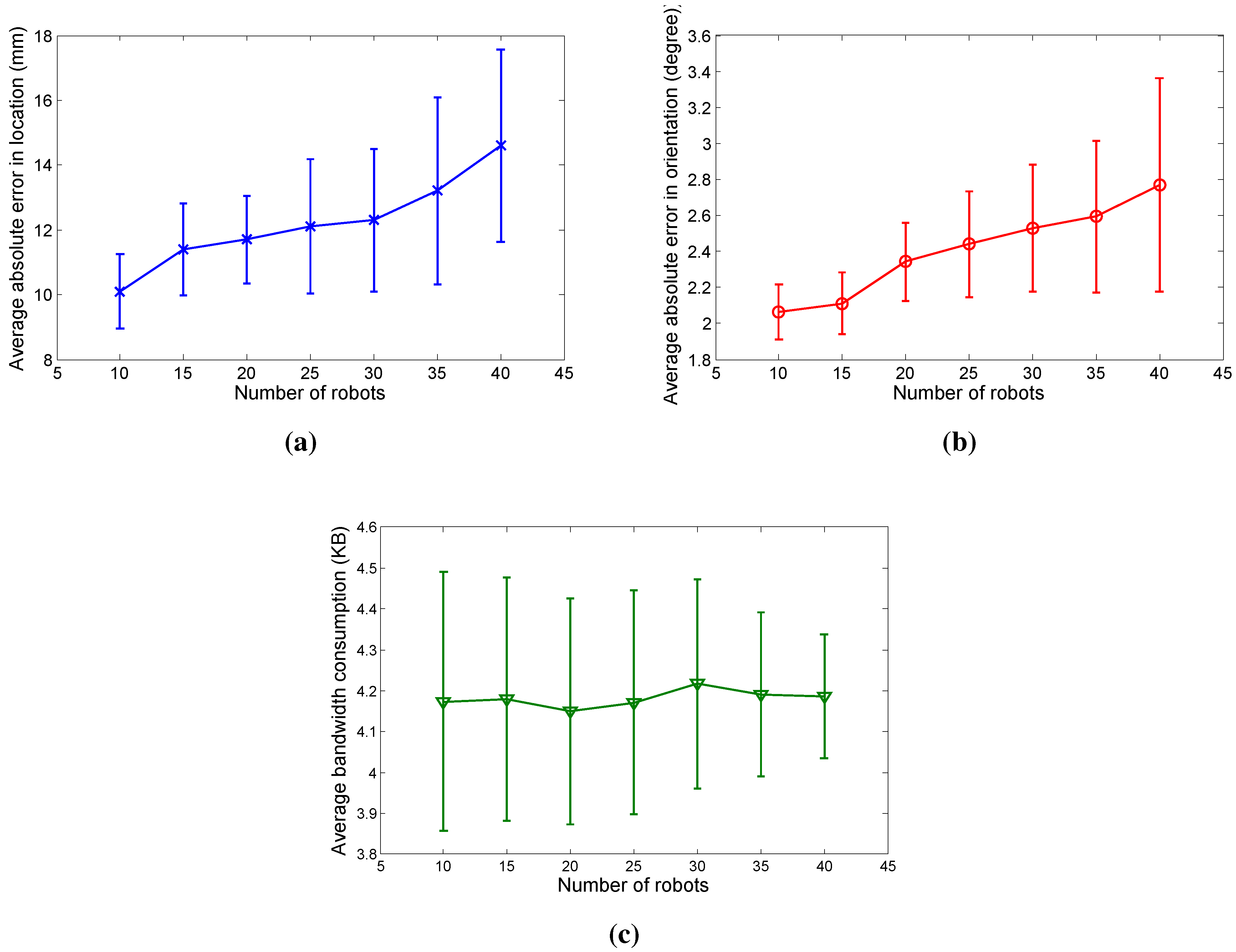
4.2. Simulation Experiments

5. Conclusions
Author Contributions
Conflicts of Interest
References
- Oyekan, J.; Hu, H. Ant Robotic Swarm for Visualizing Invisible Hazardous Substances. Robotics 2013, 2, 1–18. [Google Scholar] [CrossRef]
- Parker, L.E. Distributed Algorithms for Multi-Robot Observation of Multiple Moving Targets. Auton. Robots 2002, 12, 231–255. [Google Scholar] [CrossRef]
- Delle Fave, F.; Canu, S.; Iocchi, L.; Nardi, D.; Ziparo, V. Multi-Objective Multi-Robot Surveillance. In Proceedings of the 4th International Conference on Autonomous Robots and Agents, Wellington, New Zealand, 10–12 February 2009; pp. 68–73.
- Karakaya, M.; Qi, H. Collaborative Localization in Visual Sensor Networks. ACM Trans. Sens. Netw. 2014, 10, 18:1–18:24. [Google Scholar] [CrossRef]
- Stroupe, A.W.; Martin, M.C.; Balch, T. Distributed Sensor Fusion for Object Position Estimation by Multi-Robot Systems. In Proceedings of the IEEE International Conference on Robotics and Automation, Seoul, Korea, 21-26 May 2001; Volume 2, pp. 1092–1098.
- Soto, C.; Song, B.; Roy-Chowdhury, A.K. Distributed Multi-Target Tracking in a Self-Configuring Camera Network. In Proceedings of the IEEE Conference on Computer Vision and Pattern Recognition, Miami, FL, USA, 20–25 June 2009; pp. 1486–1493.
- Xu, Y.; Qi, H. Mobile Agent Migration Modeling and Design for Target Tracking in Wireless Sensor Networks. Ad Hoc Netw. 2008, 6, 1–16. [Google Scholar] [CrossRef]
- Dong, W. Tracking Control of Multiple-Wheeled Mobile Robots With Limited Information of a Desired Trajectory. IEEE Trans. Robot. 2012, 28, 262–268. [Google Scholar] [CrossRef]
- Dong, W.; Chen, C.; Xing, Y. Distributed estimation-based tracking control of multiple uncertain non-linear systems. Int. J. Syst. Sci. 2014, 45, 2088–2099. [Google Scholar] [CrossRef]
- Dong, W.; Djapic, V. Leader-following control of multiple nonholonomic systems over directed communication graphs. Int. J. Syst. Sci. 2014. [Google Scholar] [CrossRef]
- Samperio, R.; Hu, H. Real-Time Landmark Modelling for Visual-Guided Walking Robots. Int. J. Comput. Appl. Technol. 2011, 41, 253–261. [Google Scholar] [CrossRef]
- Gil, A.; Reinoso, Ó.; Ballesta, M.; Juliá, M. Multi-Robot Visual SLAM Using a Rao-Blackwellized Particle Filter. Robot. Auton. Syst. 2010, 58, 68–80. [Google Scholar] [CrossRef]
- Chow, J.C.; Lichti, D.D.; Hol, J.D.; Bellusci, G.; Luinge, H. IMU and Multiple RGB-D Camera Fusion for Assisting Indoor Stop-and-Go 3D Terrestrial Laser Scanning. Robotics 2014, 3, 247–280. [Google Scholar] [CrossRef]
- Zhang, Z. A Flexible New Technique for Camera Calibration. IEEE Trans. Pattern Anal. Mach. Intell. 2000, 22, 1330–1334. [Google Scholar] [CrossRef]
- Kitahara, I.; Saito, H.; Akimichi, S.; Ono, T.; Ohta, Y.; Kanade, T. Large-scale virtualized reality. In Proceedings of the International Conference on Computer Vision and Pattern Recognition, Kauai, HI, USA, 8–14 December 2001.
- Chen, X.; Davis, J.; Slusallek, P. Wide Area Camera Calibration Using Virtual Calibration Objects. In Proceedings of the IEEE Conference on Computer Vision and Pattern Recognition, Hilton Head, SC, USA, 13–15 June 2000; Volume 2, pp. 520–527.
- Svoboda, T.; Hug, H.; Gool, L.J.V. ViRoom-Low Cost Synchronized Multicamera System and Its Self-calibration. In Proceedings of the 24th DAGM Symposium on Pattern Recognition, Zurich, Switzerland, 16–18 September 2002; pp. 515–522.
- Svoboda, T.; Martinec, D.; Pajdla, T. A Convenient Multi-Camera Self-Calibration for Virtual Environments. Teleoperators Virtual Environ. 2005, 14, 407–422. [Google Scholar] [CrossRef]
- Hörster, E.; Lienhart, R. Calibrating and Optimizing Poses of Visual Sensors in Distributed Platforms. Multimed. Syst. 2006, 12, 195–210. [Google Scholar] [CrossRef]
- Läbe, T.; Förstner, W. Automatic Relative Orientation of Images. In Proceedings of the 5th Turkish-German Joint Geodetic Days, Berlin, Germany, 28–31 March 2006; Volume 29, p. 31.
- Rodehorst, V.; Heinrichs, M.; Hellwich, O. Evaluation of Relative Pose Estimation Methods for Multi-Camera Setups. Int. Arch. Photogram. Remote Sens. 2008, 135–140. [Google Scholar]
- Jaspers, H.; Schauerte, B.; Fink, G.A. Sift-Based Camera Localization Using Reference Objects for Application in Multi-camera Environments and Robotics. In Proceedings of the International Conference on Pattern Recognition Applications and Methods, vilamoura, portugal, 6–8 February 2012; pp. 330–336.
- Aslan, C.T.; Bernardin, K.; Stiefelhagen, R.; others. Automatic Calibration of Camera Networks Based on Local Motion Features. In Proceedings of the Workshop on Multi-Camera and Multi-Modal Sensor Fusion Algorithms and Applications, Marseille, France, October 2008.
- Devarajan, D.; Radke, R.J. Distributed Metric Calibration of Large Camera Networks. In Proceedings of the First Workshop on Broadband Advanced Sensor Networks (BASENETS), San Jose, CA, USA, 25 October 2004; Volume 3, pp. 5–24.
- Kurillo, G.; Li, Z.; Bajcsy, R. Wide-Area External Multi-Camera Calibration Using Vision Graphs and Virtual Calibration Object. In Proceedings of the Second ACM/IEEE International Conference on Distributed Smart Cameras, Stanford, CA, USA, 7–11 September 2008; pp. 1–9.
- Cheng, Z.; Devarajan, D.; Radke, R.J. Determining Vision Graphs for Distributed Camera Networks Using Feature Digests. EURASIP J. Appl. Signal Process. 2007, 2007, 220–220. [Google Scholar] [CrossRef]
- Vergés-Llahı, J.; Moldovan, D.; Wada, T. A New Reliability Measure for Essential Matrices Suitable in Multiple View Calibration. In Proceedings of the International Joint Conference on Computer Vision, Imaging and Computer Graphics Theory and Applications, Funchal, Portugal, 22–25 January 2008; pp. 114–121.
- Bajramovic, F.; Denzler, J. Global Uncertainty-based Selection of Relative Poses for Multi Camera Calibration. In Proceedings of the British Machine Vision Conference, Leeds, UK, 1–4 September 2008; pp. 1–10.
- Bajramovic, F.; Brückner, M.; Denzler, J. An Efficient Shortest Triangle Paths Algorithm Applied to Multi-Camera Self-Calibration. J. Math. Imaging Vis. 2012, 43, 89–102. [Google Scholar] [CrossRef]
- Brückner, M.; Bajramovic, F.; Denzler, J. Intrinsic and Extrinsic Active Self-Calibration of Multi-Camera Systems. Mach. Vis. Appl. 2014, 25, 389–403. [Google Scholar] [CrossRef]
- Wireless Sensor and Robot Networks Laboratory (WSRNLab). Available online: http://wsrnlab.ecse.monash.edu.au (accessed on 1 December 2014).
- Beagleboard-xM System Reference Manual. Available online: http://beagleboard.org/static/ (accessed on 1 December 2014).
- Ubuntu Server for ARM Processor Family. Available online: http://www.ubuntu.com/download/server/arm (accessed on 1 December 2014).
- OpenKinect Library. Available online: http://openkinect.org (accessed on 1 December 2014).
- OpenCV: Open Source Computer Vision Library. Available online: http://opencv.org (accessed on 1 December 2014).
- libCVD-Computer Vision Library. Available online: http://www.edwardrosten.com/cvd/ (accessed on 1 December 2014).
- Arieli, Y.; Freedman, B.; Machline, M.; Shpunt, A. Depth Mapping Using Projected Patterns. U.S. Patent 8,150,142, 2012. [Google Scholar]
- Butler, D.A.; Izadi, S.; Hilliges, O.; Molyneaux, D.; Hodges, S.; Kim, D. Shake’n’Sense: Reducing Interference for Overlapping Structured Light Depth Cameras. In Proceedings of the SIGCHI Conference on Human Factors in Computing Systems, ACM, Austin, Texas, 5–10 May 2012; pp. 1933–1936.
- Khoshelham, K. Accuracy Analysis of Kinect Depth Data. In Proceedings of the ISPRS Workshop Laser Scanning, Calgary, Canada, 29–31 August 2011; Volume 38, p. W12.
- Stowers, J.; Hayes, M.; Bainbridge-Smith, A. Altitude Control of a Quadrotor Helicopter Using Depth Map from Microsoft Kinect Sensor. In Proceedings of the 2011 IEEE International Conference on Mechatronics, Istanbul, Turkey, 13–15 April 2011; pp. 358–362.
- Khoshelham, K.; Elberink, S.O. Accuracy and Resolution of Kinect Depth Data for Indoor Mapping Applications. Sensors 2012, 12, 1437–1454. [Google Scholar] [CrossRef] [PubMed]
- Rosten, E.; Drummond, T. Machine Learning for High-Speed Corner Detection. In Computer Vision–ECCV 2006; Springer: Berlin/Heidelberg, Germany, 2006; pp. 430–443. [Google Scholar]
- Rosten, E.; Porter, R.; Drummond, T. Faster and Better: A Machine Learning Approach to Corner Detection. IEEE Trans. Pattern Anal. Mach. Intell. 2010, 32, 105–119. [Google Scholar] [CrossRef] [PubMed]
- Rublee, E.; Rabaud, V.; Konolige, K.; Bradski, G. ORB: An Efficient Alternative to SIFT or SURF. In Proceedings of the 2011 IEEE International Conference on Computer Vision, Barcelona, Spain, 6–13 November 2011; pp. 2564–2571.
- Izadi, S.; Kim, D.; Hilliges, O.; Molyneaux, D.; Newcombe, R.; Kohli, P.; Shotton, J.; Hodges, S.; Freeman, D.; Davison, A.; Fitzgibbon, A. Kinectfusion: Real-Time 3D Reconstruction and Interaction Using a Moving Depth Camera. In Proceedings of the UIST, Santa Barbara, CA, USA, 16–19 October 2011; pp. 559–568.
- Lui, W.; Tang, T.; Drummond, T.; Li, W.H. Robust Egomotion Estimation Using ICP in Inverse Depth Coordinates. In Proceedings of the 2012 IEEE International Conference on Robotics and Automation (ICRA), Saint Paul, MN, USA, 14–18 May 2012; pp. 1671–1678.
- Wang, X.; Şekercioğlu, Y.A.; Drummond, T. A Real-Time Distributed Relative Pose Estimation Algorithm for RGB-D Camera Equipped Visual Sensor Networks. In Proceedings of the 7th ACM/IEEE International Conference on Distributed Smart Cameras (ICDSC 2013), Palm Springs, CA, USA, 29 October–1 November 2013.
- Zou, Y.; Chen, W.; Wu, X.; Liu, Z. Indoor Localization and 3D Scene Reconstruction for Mobile Robots Using the Microsoft Kinect Sensor. In Proceedings of the 10th IEEE International Conference on Industrial Informatics, Beijing, China, 25–27 July 2012; pp. 1182–1187.
- Wang, H.; Mou, W.; Ly, M.H.; Lau, M.; Seet, G.; Wang, D. Mobile Robot Egomotion Estimation Using RANSAC-Based Ceiling Vision. In Proceedings of the 24th Chinese Control and Decision Conference, Taiyuan, China, 23–25 May 2012; pp. 1939–1943.
- Henry, P.; Krainin, M.; Herbst, E.; Ren, X.; Fox, D. RGB-D Mapping: Using Kinect-Style Depth Cameras for Dense 3D Modeling of Indoor Environments. Int. J. Robot. Res. 2012, 31, 647–663. [Google Scholar] [CrossRef]
- Endres, F.; Hess, J.; Engelhard, N.; Sturm, J.; Cremers, D.; Burgard, W. An Evaluation of the RGB-D SLAM System. In Proceedings of the IEEE International Conference on Robotics and Automation (ICRA 2012), Saint Paul, MN, USA, 14–18 May 2012; pp. 1691–1696.
- Holland, P.W.; Welsch, R.E. Robust regression using iteratively reweighted least-squares. Commun. Stat.-Theory Meth. 1977, 6, 813–827. [Google Scholar] [CrossRef]
- Mori, Y.; Fukushima, N.; Fujii, T.; Tanimoto, M. View Generation with 3D Warping Using Depth Information for FTV. In Proceedings of the 3DTV Conference: The True Vision-Capture, Transmission and Display of 3D Video, Potsdam, Germany, 4–6 May 2008; pp. 229–232.
© 2014 by the authors; licensee MDPI, Basel, Switzerland. This article is an open access article distributed under the terms and conditions of the Creative Commons Attribution license (http://creativecommons.org/licenses/by/4.0/).
Share and Cite
Wang, X.; Şekercioğlu, Y.A.; Drummond, T. Vision-Based Cooperative Pose Estimation for Localization in Multi-Robot Systems Equipped with RGB-D Cameras. Robotics 2015, 4, 1-22. https://doi.org/10.3390/robotics4010001
Wang X, Şekercioğlu YA, Drummond T. Vision-Based Cooperative Pose Estimation for Localization in Multi-Robot Systems Equipped with RGB-D Cameras. Robotics. 2015; 4(1):1-22. https://doi.org/10.3390/robotics4010001
Chicago/Turabian StyleWang, Xiaoqin, Y. Ahmet Şekercioğlu, and Tom Drummond. 2015. "Vision-Based Cooperative Pose Estimation for Localization in Multi-Robot Systems Equipped with RGB-D Cameras" Robotics 4, no. 1: 1-22. https://doi.org/10.3390/robotics4010001