Robust Nonlinear Regulation of Limit Cycle Oscillations in UAVs Using Synthetic Jet Actuators

Abstract

In this paper, a synthetic jet actuators (SJA)-based nonlinear robust controller is developed, which is capable of completely suppressing limit cycle oscillations (LCO) in UAV systems with parametric uncertainty in the SJA dynamics and unmodeled external disturbances. Specifically, the control law compensates for uncertainty in an input gain matrix, which results from the unknown airflow dynamics generated by the SJA. Challenges in the control design include compensation for input-multiplicative parametric uncertainty in the actuator dynamic model. The result was achieved via innovative algebraic manipulation in the error system development, along with a Lyapunov-based robust control law. A rigorous Lyapunov-based stability analysis is utilized to prove asymptotic LCO suppression, considering a detailed dynamic model of the pitching and plunging dynamics. Numerical simulation results are provided to demonstrate the robustness and practical performance of the proposed control law.

1. Introduction

There has recently been a surge of interest in the design and application of unmanned aerial vehicles (UAVs). These UAVs can be used in numerous civilian applications, such as urban reconnaissance, package delivery, and area mapping. Besides, UAVs are utilized in various military applications as well. One of the biggest challenges involved in the autonomous operation of UAVs is in the design of flight tracking controllers for UAVs operating in uncertain and possibly adverse conditions. In particular, suppression of limit cycle oscillations (LCO) (or flutter) is an important concern in UAV tracking control design. This is especially true for applications involving smaller, lightweight UAV systems, where the aircraft wings are more susceptible to LCO. These engineering challenges necessitate the utilization of UAV flight controllers, which achieve accurate flight tracking in the presence of dynamic uncertainty while simultaneously suppressing LCO. Moreover, as practical considerations motivate the implementation of smaller UAVs, there is a growing need for UAV flight control designs that do not require heavy mechanical deflection surfaces.

LCO refer to “flutter” behaviors in UAV wings that manifest themselves as constant-amplitude oscillations [1], which result from nonlinearities inherent in the aeroelastic dynamics of the UAV system [2]. Due to these behaviors, the LCO would surpass the limiting safe flight boundaries of an aircraft [3] and could potentially lead to structural damage and catastrophes. Control applications for LCO suppression are often developed (e.g., see [4,5,6]) using mechanical deflection surfaces (e.g. flaps, ailerons, rudders, and elevators). However, when dealing with small UAVs, practical engineering considerations and physical constraints can preclude the addition of the large, heavy moving parts that are required for the installation of deflection surfaces. To address this challenge, the use of synthetic jet actuators (SJA) in UAV flight control systems is becoming popular as a practical alternative to mechanical deflection surfaces.

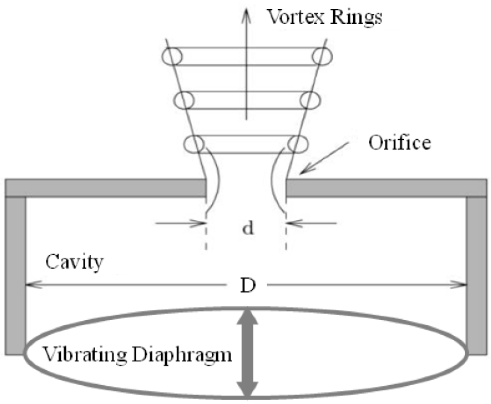
The design and application of SJA has recently increased by virtue of their capability to achieve momentum transfer with zero-net mass-flux. This beneficial feature eliminates the need for an external fuel supply, since the working substance is simply the gas (i.e., air) that is already present in the environment of operation [7]. This makes SJA an attractive option in UAV applications, because of the significant reduction in the size of the required equipment. The SJA synthesize the jet flow through the alternating suction and ejection of fluid through an aperture, which is produced via pressure oscillations in a cavity [8] as shown in Figure 1. The pressure oscillations can be generated using various methods, including pistons in the SJA orifices [3] or piezoelectric diaphragms [7,9]. SJA can achieve boundary-layer flow control near the surface of a UAV wing [10], since they can provide instant actuation, unlike conventional mechanical control surfaces. In addition, SJA can expand the usable range of angle of attack, resulting in improved UAV maneuverability [11].

Recently developed nonlinear control methods using SJA typically utilize neural networks and/or complex fluid dynamics computations in the feedback loop (e.g., see [9,10,12,13,14,15,16,17,18,19,20,21]). While such approaches have been shown to yield good SJA-based control performance, they can require increased computational resources, which might not be available in small UAV applications. Adaptive control approaches have been applied to linear time-invariant (LTI) dynamic models to compensate for SJA nonlinearities and external disturbances [13]. Adaptive inverse control schemes are another popularly utilized method to compensate for the actuator nonlinearity inherent in SJA [9,14,15,16,17]. A robust tracking control method is proposed in [7], which builds on results similar to [9,14,15,16,17], to compensate for the SJA nonlinearity at a reduced computational cost. The aforementioned approaches have been shown to achieve good flight tracking performance using SJA; however, nonlinear control approaches have not as often been applied to SJA-based LCO suppression.

Figure 1. Schematic layout of a synthetic jet actuator.

Figure 1. Schematic layout of a synthetic jet actuator.

In this paper, an SJA-based nonlinear robust controller is developed, which is capable of completely suppressing LCO in UAV systems with uncertain dynamics. This difficulty was handled via innovative algebraic manipulation in the error system development, along with a Lyapunov-based robust control law. A salient feature about this robust control law is that its structure is continuous, and so bounded disturbances can be asymptotically rejected without the need for infinite bandwidth. A rigorous Lyapunov-based stability analysis is utilized to prove asymptotic pitching and plunging regulation, considering a detailed dynamic model of the pitching and plunging dynamics. Numerical simulation results are provided to demonstrate the performance of the proposed control law.

2. Dynamic Model and Properties

The equation describing LCO in an airfoil approximated as a 2-dimensional thin plate can be expressed as

$$M_s\ddot{p}+C_s\dot{p}+F\left(p\right)p=\left[\begin{array}{c}-Lift\hfill \\ Moment\hfill \end{array}\right]$$

(1)

where the coefficients $M_s$, $C_s\in {\mathbb{R}}^{2\times 2}$ denote the structural mass and damping matrices, $F\left(p\right)\in {\mathbb{R}}^{2\times 2}$ is a nonlinear stiffness matrix, and $p\left(t\right)\in {\mathbb{R}}^2$ denotes the state vector. In Equation (1), $p\left(t\right)$ is explicitly defined as

$$p=\left[\begin{array}{c}h\hfill \\ \alpha \hfill \end{array}\right]$$

(2)

where $h\left(t\right)$, $\alpha \left(t\right)\in \mathbb{R}$ denote the plunging [meters] and pitching [radians] displacements describing the LCO effects. Also in Equation (1), the structural linear mass matrix $M_s$ [22]

$$M_s=\left[\begin{array}{cc}m& S_{\alpha }\\ S_{\alpha }& I_{\alpha }\end{array}\right]$$

(3)

where the parameters $S_{\alpha },$ $I_{\alpha }\in \mathbb{R}$ are the static moment and moment of inertia, respectively. The structural linear damping matrix is described as

$$C_s=2\left[\begin{array}{cc}{\zeta }_h\sqrt{k_{h}m}& 0\\ 0& {\zeta }_a\sqrt{k_{\alpha }{I}_{\alpha }}\end{array}\right]$$

(4)

where the parameters ${\zeta }_h$, ${\zeta }_{\alpha }\in \mathbb{R}$ are the damping logarithmic decrements for plunging and pitching, and $m\in \mathbb{R}$ is the mass of the wing, or in this case, a flat plate. The nonlinear stiffness matrix utilized in this study is

$$F\left(p\right)=\left[\begin{array}{cc}{k}_h& 0\\ 0& k_{\alpha }+k_{{\alpha }^3}{\alpha }^2\end{array}\right]$$

(5)

where $k_{\alpha },$ $k_{{\alpha }^3}\in \mathbb{R}$ denote structural resistances to pitching (linear and nonlinear) and $k_h\in \mathbb{R}$ is the structural resistance to plunging.

In Equation (1), the total lift and moment are explicitly defined as

$$\begin{array}{c}\left[\begin{array}{c}-Lift\\ Moment\end{array}\right]=\left[\begin{array}{c}-(L+L_{v_j})\\ (M+M_{v_j})\end{array}\right]\\ =M_a\ddot{p}+C_a\dot{p}+K_{a}p+L_{\eta }\eta +Bu\end{array}$$

(6)

where $L_{vj}\left(t\right),M_{vj}\left(t\right)\in \mathbb{R}$ denote the equivalent control force and moment generated by the jth SJA, and $L\left(t\right)$, $M\left(t\right)\in \mathbb{R}$ are the aerodynamic lift and moment due to the 2 degree-of-freedom motion [10]. In Equation (6), $\eta \left(t\right)\in {\mathbb{R}}^2$ denotes the aerodynamic state vector that relates the moment and lift to the structural modes. Also in Equation (6), $u\left(t\right)\in {\mathbb{R}}^2$ denotes the SJA-based control input (e.g., the SJA air velocity or acceleration), and $B\in {\mathbb{R}}^{2\times 2}$ is an uncertain constant input gain matrix that relates the control input $u\left(t\right)$ to the equivalent force and moment generated by the SJA. Also in Equation (6), the aerodynamic and mode matrices $M_a$, $C_a$, $K_a$, $L_{\eta }\in {\mathbb{R}}^{2\times 2}$ are described as

$$\begin{array}{c}{M}_a=\pi \rho b^2\left[\begin{array}{cc}-1& ba\\ ba& -b^2\left(\frac{1}{8}+a^2\right)\end{array}\right]\end{array}$$

(7)

$$\begin{array}{c}{C}_a=\pi \rho b^2\left[\begin{array}{cc}0& -U\\ 0& -Ub\left(\frac{1}{2}-a\right)\end{array}\right]\\ +2\pi \rho Ub\varphi \left(0\right)\left[\begin{array}{cc}-1& -b\left(\frac{1}{2}-a\right)\\ b\left(\frac{1}{2}+a\right)& b^2\left(\frac{1}{2}+a\right)\left(\frac{1}{2}-a\right)\end{array}\right]\end{array}$$

(8)

$$\begin{array}{c}{K}_a=2\pi \rho Ub\varphi \left(0\right)\left[\begin{array}{cc}0& -U\\ 0& b\left(\frac{1}{2}+a\right)U\end{array}\right]\end{array}$$

(9)

$$\begin{array}{c}{L}_{\eta }=2\pi \rho Ub\left[\begin{array}{cc}{a}_1{b}_1& a_2{b}_2\\ -b\left({\displaystyle \frac{1}{2}}+a\right)a_1{b}_1& -b\left({\displaystyle \frac{1}{2}}+a\right)a_2{b}_2\end{array}\right]\end{array}$$

(10)

where $\varphi \left(0\right)$ is the Wagner solution function at 0, and the parameters $a_1$, $b_1$, $a_2$, $b_2\in \mathbb{R}$ are the Wagner coefficients. In addition, $a,b\in \mathbb{R}$ denote the relative locations of the rotational axis from the mid-chord and the semi-chord, respectively. The aerodynamic state variables are governed by [22]

$$\dot{\eta }=C_{\eta }\dot{p}+K_{\eta }p+S_{\eta }\eta$$

(11)

The aerodynamic state matrices in Equation (11), $C_{\eta }$, $K_{\eta }$, $S_{\eta }\in {\mathbb{R}}^{2\times 2}$, are explicitly defined as

$$\begin{array}{c}{C}_{\eta }={\displaystyle \frac{U}{b}}\left[\begin{array}{cc}-1& -b\left({\displaystyle \frac{1}{2}}-a\right)\\ -1& -b\left({\displaystyle \frac{1}{2}}-a\right)\end{array}\right]\end{array}$$

(12)

$$\begin{array}{c}{K}_{\eta }={\displaystyle \frac{U}{b}}\left[\begin{array}{cc}0& -U\\ 0& -U\end{array}\right]\end{array}$$

(13)

$$\begin{array}{c}{S}_{\eta }={\displaystyle \frac{U}{b}}\left[\begin{array}{cc}-b_1& 0\\ 0& -b_2\end{array}\right].\end{array}$$

(14)

By substituting Equation (6) into Equation (1), the LCO dynamics can be expressed as

$$\ddot{p}=-M^{-1}C\dot{p}-M^{-1}Kp+M^{-1}{L}_{\eta }\eta +M^{-1}Bu$$

(15)

where $C=C_s-C_a$, $K=F\left(p\right)-K_a$, and $M=M_s-M_a$. By making the definitions $x_1\left(t\right)=h\left(t\right)$, $x_2\left(t\right)=\alpha \left(t\right)$, $x_3\left(t\right)=\dot{h}\left(t\right)$, $x_4\left(t\right)=\dot{\alpha }\left(t\right)$, $x_5\left(t\right)={\eta }_1\left(t\right)$, and $x_6\left(t\right)={\eta }_2\left(t\right)$, the dynamic equation in Equation (15) can be expressed in state form as

$$\dot{x}=A\left(x\right)x+\overline{B}u$$

(16)

where $x\left(t\right)\in {\mathbb{R}}^6$ is the state vector, $A\left(x\right)\in {\mathbb{R}}^{6\times 6}$ is the state matrix (state-dependent). In Equation (16), the input gain matrix $\overline{B}\in {\mathbb{R}}^{6\times 2}$ is defined as

$$\overline{B}=\left[\begin{array}{c}{0}_{2\times 2}\\ M^{-1}B\\ 0_{2\times 2}\end{array}\right]$$

(17)

where $0_{2\times 2}$ denotes a $2\times 2$ matrix of zeros. The structure of the input gain matrix in Equation (17) results from the fact that the control input $u\left(t\right)$ only directly affects $\ddot{h}\left(t\right)$ and $\ddot{\alpha }\left(t\right)$.

3. Control Development

The objective is to design the control signal $u\left(t\right)$ to regulate the plunge and pitching dynamics (i.e., $h\left(t\right),\alpha \left(t\right)$) to zero. To facilitate the control design, the expression in Equation (15) is rewritten as

$$M\ddot{p}=g(h,\alpha ,\eta )+Bu$$

(18)

where $g(h,\alpha ,\eta )$ is an unknown, unmeasurable auxiliary function.

Remark 1. Based on the open-loop error dynamics in Equation (18), one of the control design challenges is that the control input $u\left(t\right)$ is premultiplied by the uncertain matrix B. In the following control development and stability analysis, it will be assumed that the matrix B is uncertain, and the robust control law will be designed with a constant feedforward estimate of the uncertain matrix. The simulation results demonstrate the capability of the robust control law to compensate for the input matrix uncertainty without the need for online parameter estimation or function approximators.

To quantify the control objective, a regulation error $e_1\left(t\right)\in {\mathbb{R}}^2$ and auxiliary tracking error variables $e_2\left(t\right),$ $r\left(t\right)\in {\mathbb{R}}^2$ are defined as

$$\begin{array}{ccc}\hfill e_1& =& p-p_d\hfill \end{array}$$

(19)

$$\begin{array}{ccc}\hfill e_2& =& {\dot{e}}_1+{\alpha }_1{e}_1\hfill \end{array}$$

(20)

$$\begin{array}{ccc}\hfill r& =& {\dot{e}}_2+{\alpha }_2{e}_2\hfill \end{array}$$

(21)

where ${\alpha }_1,{\alpha }_2>0\in {\mathbb{R}}^{+}$ are user-defined control gains, and the desired plunging and pitching states $p_d={\left[h,a\right]}^T={\left[0,0\right]}^T$ for the plunging and pitching suppression objective. To facilitate the following analysis, Equation (21) is premultiplied by M and the time derivative is calculated as

$$M\dot{r}=M{\ddot{e}}_2+{\alpha }_{2}M{\dot{e}}_2$$

(22)

After using Equations (18)–(21), the open-loop error dynamics are obtained as

$$M\dot{r}=\tilde{N}+N_d+B\dot{u}-e_2$$

(23)

where the unknown, unmeasurable auxiliary functions $\tilde{N}\left(e_1,e_2,r\right)$, $N_d\left(p_d,{\stackrel{⃛}{p}}_d\right)\in {\mathbb{R}}^2$ are defined as

$$\begin{array}{ccc}\hfill \tilde{N}& \triangleq & \dot{g}(p,\eta )-\dot{g}\left(p_d,\eta \right)+{\alpha }_1\left(r-{\alpha }_2{e}_2-{\alpha }_1{e}_2+{\alpha }_1^2{e}_1\right)\hfill \\ & & +{\alpha }_{2}M\left(r-{\alpha }_2{e}_2\right)+e_2\hfill \end{array}$$

(24)

$$\begin{array}{ccc}\hfill N_d& \triangleq & -{\stackrel{⃛}{p}}_d+\dot{g}\left(p_d,\eta \right)\hfill \end{array}$$

(25)

The motivation for defining the auxiliary functions in Equations (24) and (25) is based on the fact that the following inequalities can be developed:

$$\parallel \tilde{N}\parallel \le {\rho }_0\parallel z\parallel ,\parallel N_d\parallel \le {\zeta }_{N_d},\parallel {\dot{N}}_d\parallel \le {\zeta }_{{\dot{N}}_d}$$

(26)

where ${\rho }_0$, ${\zeta }_{N_d}$, ${\zeta }_{{\dot{N}}_d}\in {\mathbb{R}}^{+}$ are known bounding constants, and $z\left(t\right)\in {\mathbb{R}}^6$ is defined as

$$z\triangleq {\left[\begin{array}{ccc}{e}_1^T& e_2^T& r^T\end{array}\right]}^T$$

(27)

Based on the open-loop error dynamics in Equation (23), the control input is designed via

$$\dot{u}={\widehat{B}}^{-1}(-(k_s+I_{2\times 2})r-\beta sgn\left(e_2\left(t\right)\right)$$

(28)

where $k_s$, $\beta \in {\mathbb{R}}^{2\times 2}$ denote constant, positive definite, diagonal control gain matrices, and $I_{2\times 2}$ denotes a $2\times 2$ identity matrix. In Equation (28), $\widehat{B}\in {\mathbb{R}}^{2\times 2}$ denotes a constant, feedforward “best guess” estimate of the uncertain input gain matrix B. Note that the control input $u\left(t\right)$ does not depend on the unmeasurable acceleration term $r\left(t\right)$, since Equation (28) can be directly integrated to show that $u\left(t\right)$ requires measurements of $e_1\left(t\right)$ and $e_2\left(t\right)$ only.

To facilitate the following stability proof, the control gain matrix β in Equation (28) is selected to satisfy the sufficient condition

$${\lambda }_{min}\left(\beta \right)>{\zeta }_{N_d}+\frac{1}{{\alpha }_2}{\zeta }_{{\dot{N}}_d}$$

(29)

where ${\lambda }_{min}\left(·\right)$ denotes the minimum eigenvalue of the argument. After substituting Equation (28) into Equation (23), the closed-loop error dynamics are obtained as

$$M\dot{r}=\tilde{N}+N_d-(k_s+I_{n\times n})r+\beta sgn\left(e_2\left(t\right)\right)-e_2$$

(30)

To reduce the complexity of the following stability analysis, it is assumed that the product $B{\widehat{B}}^{-1}$ is equal to identity. It can be proven that asymptotic regulation can be achieved for the case where the feedforward estimate $\widehat{B}$ is within some prescribed finite range of the actual matrix B. The proof including the uncertainty in B is lengthy and is omitted here for brevity. The complete proof can be found in [23,24]. The following simulation results demonstrate the performance of the controller in the presence of uncertainty in the input gain matrix $B.$

3.1. Stability Analysis

Theorem 1. The controller given in Equation (28) ensures asymptotic regulation of pitching and plunging displacements in the sense that

$$∥e_1\left(t\right)∥\to 0ast\to \infty$$

(31)

provided the control gain $k_s$ is selected sufficiently large, and β is selected according to the sufficient condition in Equation (29).

Lemma 1. To facilitate the following proof, let $\mathcal{D}\subset {\mathbb{R}}^7$ be a domain containing $w\left(t\right)=0$, where $w\left(t\right)\in {\mathbb{R}}^7$ is defined as

$$w\left(t\right)\triangleq {\left[\begin{array}{cc}{z}^T& \sqrt{P\left(t\right)}\end{array}\right]}^T$$

(32)

In Equation (32), the auxiliary function $P\left(t\right)\in \mathbb{R}$ is the generalized solution to the differential equation

$$\begin{array}{c}\dot{P}\left(t\right)=-L\left(t\right)\end{array}$$

(33)

$$\begin{array}{c}P\left(0\right)=\beta ∥e_2\left(0\right)∥-N_d^T\left(0\right)e_2\left(0\right)\end{array}$$

(34)

where the auxiliary function $L\left(t\right)\in \mathbb{R}$ is defined as

$$L\left(t\right)=r^T\left(N_d\left(t\right)-\beta sgn\left(e_2\right)\right)$$

(35)

Provided the sufficient condition in Equation (29) is satisfied, the following inequality can be obtained:

$${\int }_0^{t}L\left(\tau \right)d\tau \le \beta ∥e_2\left(0\right)∥-N_d^T\left(0\right)e_2\left(0\right)$$

(36)

Hence, Equation (36) can be used to conclude that $P\left(t\right)\ge 0$.

Proof 1. (See Theorem 1) Let $V(w,t):\mathcal{D}\times [0,\infty )\to \mathbb{R}$ be defined as the nonnegative function

$$V(w,t)\triangleq \frac{1}{2}{e}_1^T{e}_1+\frac{1}{2}{e}_2^T{e}_2+\frac{1}{2}{r}^{T}Mr+P$$

(37)

where $e_1\left(t\right)$, $e_2\left(t\right)$, and $r\left(t\right)$ are defined in Equations (19)–(21), respectively; and the positive definite function $P\left(t\right)$ is defined in Equation (33). The function $V(w,t)$ satisfies the inequality

$$U_1\left(w\right)\le V(w,t)\le U_2\left(w\right)$$

(38)

provided the sufficient condition introduced in Equation (29) is satisfied, where $U_1\left(w\right)$, $U_2\left(w\right)\in \mathbb{R}$ denote the positive definite functions

$$U_1\triangleq {\lambda }_1{∥w∥}^2,U_2\triangleq {\lambda }_2{∥w∥}^2$$

(39)

where ${\lambda }_1=min\left\{\frac{1}{2},{\lambda }_{min}\left(M\right)\right\}$ and ${\lambda }_2=max\left\{1,{\lambda }_{max}\left(M\right)\right\}$. After taking the time derivative of Equation (37) and utilizing Equation (20), Equation (21), Equation (30), and Equation (33), $\dot{V}(w,t)$ can be upper bounded as

$$\begin{array}{ccc}\hfill \dot{V}\left(w,t\right)& \le & -\left({\alpha }_1-\frac{1}{2}\right){∥e_1∥}^2-\left({\alpha }_2-\frac{1}{2}\right){∥e_2∥}^2-{∥r∥}^2\hfill \\ & & -k_s{∥r∥}^2+{\rho }_0∥z∥∥r∥\hfill \end{array}$$

(40)

where the bounds in Equation (26) were used, and the fact that $e_1^T{e}_2\le \frac{1}{2}{∥e_1∥}^2+\frac{1}{2}{∥e_2∥}^2$ (i.e., Young’s inequality) was utilized. After completing the squares in Equation (40), the upper bound on $\dot{V}\left(w,t\right)$ can be expressed as

$$\begin{array}{ccc}\hfill \dot{V}\left(w,t\right)& \le & -\left({\alpha }_1-\frac{1}{2}\right){∥e_1∥}^2-\left({\alpha }_2-\frac{1}{2}\right){∥e_2∥}^2-{∥r∥}^2\hfill \\ & & -k_s{\left(∥r∥-\frac{{\rho }_0}{2k_s}∥z∥\right)}^2+\frac{{\rho }_0^2}{4k_s}{∥z∥}^2\hfill \end{array}$$

(41)

Since $k_s>0$, the upper bound in Equation (41) can be expressed as

$$\dot{V}\left(w,t\right)\le -\left({\lambda }_0-\frac{{\rho }_0^2}{4k_s}\right){∥z∥}^2$$

(42)

where ${\lambda }_0\triangleq min\left\{{\alpha }_1-\frac{1}{2},{\alpha }_2-\frac{1}{2},1\right\}$.

The following expression can be obtained from Equation (42):

$$\dot{V}(w,t)\le -U\left(w\right)$$

(43)

where $U\left(w\right)=c{∥z∥}^2$, for some positive constant $c\in \mathbb{R}$, is a continuous, positive semi-definite function.

It follows directly from the Lyapunov analysis that $e_1\left(t\right),$ $e_2\left(t\right),$ $r\left(t\right)\in {\mathcal{L}}_{\infty }$. This implies that ${\dot{e}}_1\left(t\right),$ ${\dot{e}}_2\left(t\right)\in {\mathcal{L}}_{\infty }$from the definitions given in Equations (20) and (21). Given that ${\dot{e}}_1\left(t\right),$ $e_2\left(t\right)$, $r\left(t\right)\in {\mathcal{L}}_{\infty }$, it follows that ${\ddot{e}}_1\left(t\right)\in {\mathcal{L}}_{\infty }$ from Equation (21). Thus, Equation (19) can be used to prove that $p\left(t\right),$ $\dot{p}\left(t\right)$, $\ddot{p}\left(t\right)\in {\mathcal{L}}_{\infty }$. Since $p\left(t\right),$ $\dot{p}\left(t\right)$, $\ddot{p}\left(t\right)\in {\mathcal{L}}_{\infty }$, Equation (18) can be used to prove that $u\left(t\right)\in {\mathcal{L}}_{\infty }$. Since $r\left(t\right)$, $u\left(t\right)\in {\mathcal{L}}_{\infty }$, Equation (28) can be used to show that $\dot{u}\left(t\right)\in {\mathcal{L}}_{\infty }$. Given that $e_1\left(t\right),$ $e_2\left(t\right)$, $r\left(t\right),$ $\dot{u}\left(t\right)\in {\mathcal{L}}_{\infty }$, Equation (30) can be used along with Equation (26) to prove that $\dot{r}\left(t\right)\in {\mathcal{L}}_{\infty }$. Since ${\dot{e}}_1\left(t\right),{\dot{e}}_2\left(t\right),\dot{r}\left(t\right)\in {\mathcal{L}}_{\infty }$, $e_1\left(t\right),$ $e_2\left(t\right),$ $r\left(t\right)$, are uniformly continuous. Equation (27) can then be used to show that $z\left(t\right)$ is uniformly continuous. Given that $e_1\left(t\right),$ $e_2\left(t\right),$ $r\left(t\right)$ $\in {\mathcal{L}}_{\infty }$, Equation (37) and Equation (42) can be used to prove that $z\left(t\right)\in {\mathcal{L}}_{\infty }\cap {\mathcal{L}}_2$. Barbalat’s lemma [25] can now be invoked to prove that $\parallel z\left(t\right)\parallel \to 0$ as $t\to \infty$. Hence, $∥e_1\left(t\right)∥\to 0$ as $t\to \infty$ from Equation (27). Further, given that $V\left(w,t\right)$ in Equation (37) is radially unbounded, convergence of $e_1\left(t\right)$ is guaranteed, regardless of initial conditions—a global result.

4. Results and Discussion

A numerical simulation was created to demonstrate the performance of the control law developed in Equation (28). In order to develop a realistic stepping stone to high-fidelity numerical simulation results using detailed computational fluid dynamics models, the following simulation results are based on detailed dynamic parameters and specifications. The simulation is based on the dynamic model given in Equation (1) and Equation (11). The dynamic parameters utilized in the simulation are summarized in Table 1 and were obtained from [22].

Table 1. Constant simulation parameters.

$\rho =1.225\frac{kg}{m^3}$	$a=-0.24$	$U=18.25\frac{m}{s},19.5\frac{m}{s},20.5\frac{m}{s}$
$m=2.55kg$	$b=0.11m$	$v=18\frac{m}{s}$
$S_{\alpha }=10.4\times {10}^{-3}kg·m$	$a_1=0.1650$	$a_2=0.0455$
$I_{\alpha }=2.51\times {10}^{-3}kg·m$	$b_1=0.3350$	$b_2=0.3000$
$k_h=450\frac{N}{m}$	$k_{\alpha }=9.3\frac{N}{m}$	$k_{{\alpha }^3}=55\frac{N}{m}$
${\zeta }_h=5.5\times {10}^{-3}$	${\zeta }_{\alpha }=1.8\times {10}^{-2}$

Table 1. Constant simulation parameters.

$\rho =1.225\frac{kg}{m^3}$	$a=-0.24$	$U=18.25\frac{m}{s},19.5\frac{m}{s},20.5\frac{m}{s}$
$m=2.55kg$	$b=0.11m$	$v=18\frac{m}{s}$
$S_{\alpha }=10.4\times {10}^{-3}kg·m$	$a_1=0.1650$	$a_2=0.0455$
$I_{\alpha }=2.51\times {10}^{-3}kg·m$	$b_1=0.3350$	$b_2=0.3000$
$k_h=450\frac{N}{m}$	$k_{\alpha }=9.3\frac{N}{m}$	$k_{{\alpha }^3}=55\frac{N}{m}$
${\zeta }_h=5.5\times {10}^{-3}$	${\zeta }_{\alpha }=1.8\times {10}^{-2}$

The following simulation results were achieved using control gains defined as

$$\begin{array}{c}\beta =\left[\begin{array}{cc}0.001& 0\\ 0& 25\end{array}\right],k_s=\left[\begin{array}{cc}0.00001& 0\\ 0& 0.11\end{array}\right]\end{array}$$

(44)

$$\begin{array}{c}{\alpha }_1=\left[\begin{array}{cc}1& 0\\ 0& 35\end{array}\right],{\alpha }_2=\left[\begin{array}{cc}1& 0\\ 0& 35\end{array}\right]\end{array}$$

(45)

The control gains given in Equations (44) and (45) were selected based on achieving a desirable response in terms of settling time and required control effort. To test the case where the input gain matrix B is uncertain, it is assumed in the simulation that the actual value of B is the $2\times 2$ identity matrix, but the constant feedforward estimate $\widehat{B}$ used in the control law is given by

$$\widehat{B}=\left[\begin{array}{cc}0.9& 0.1\\ -0.1& 1.1\end{array}\right]$$

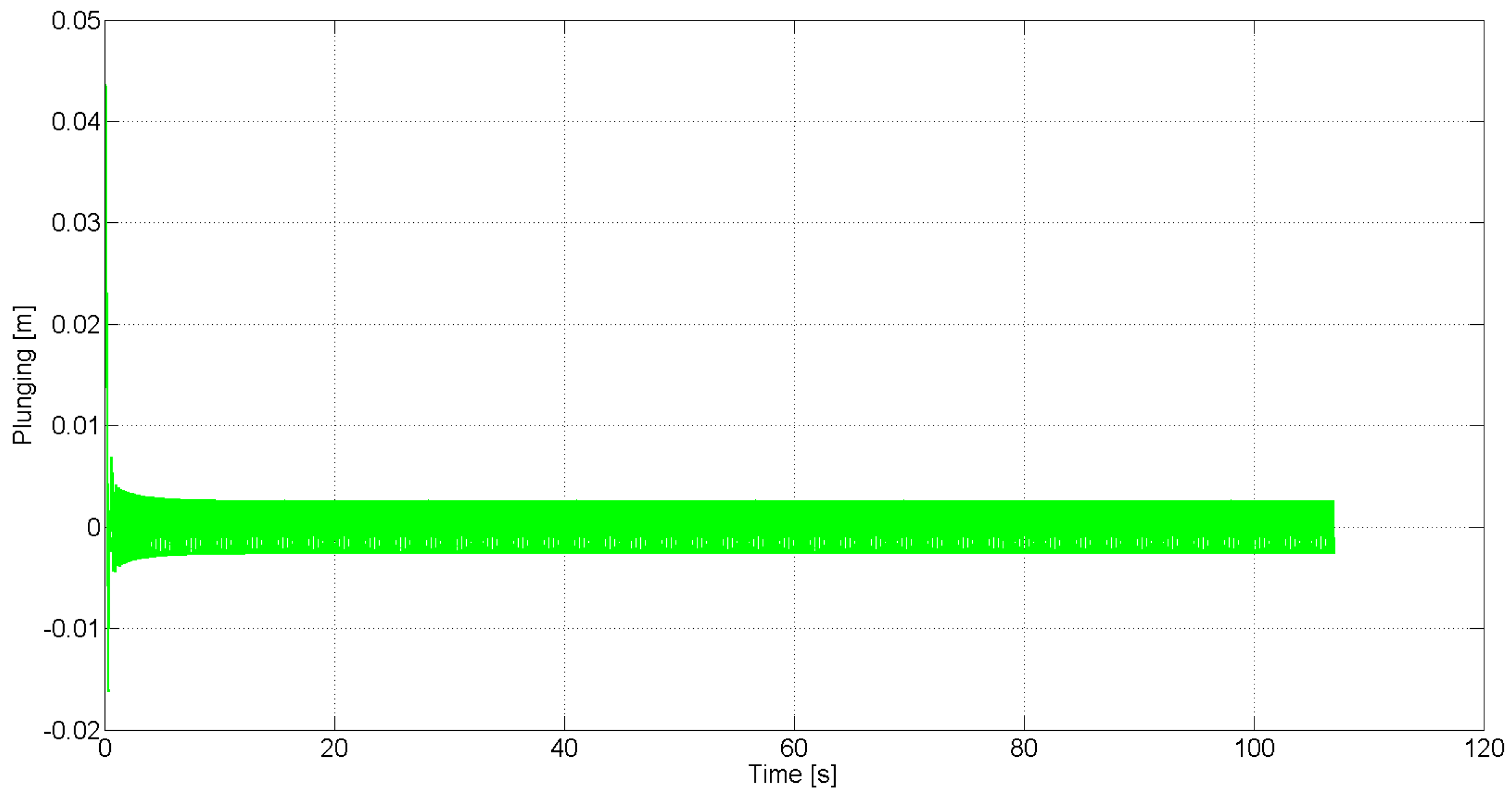
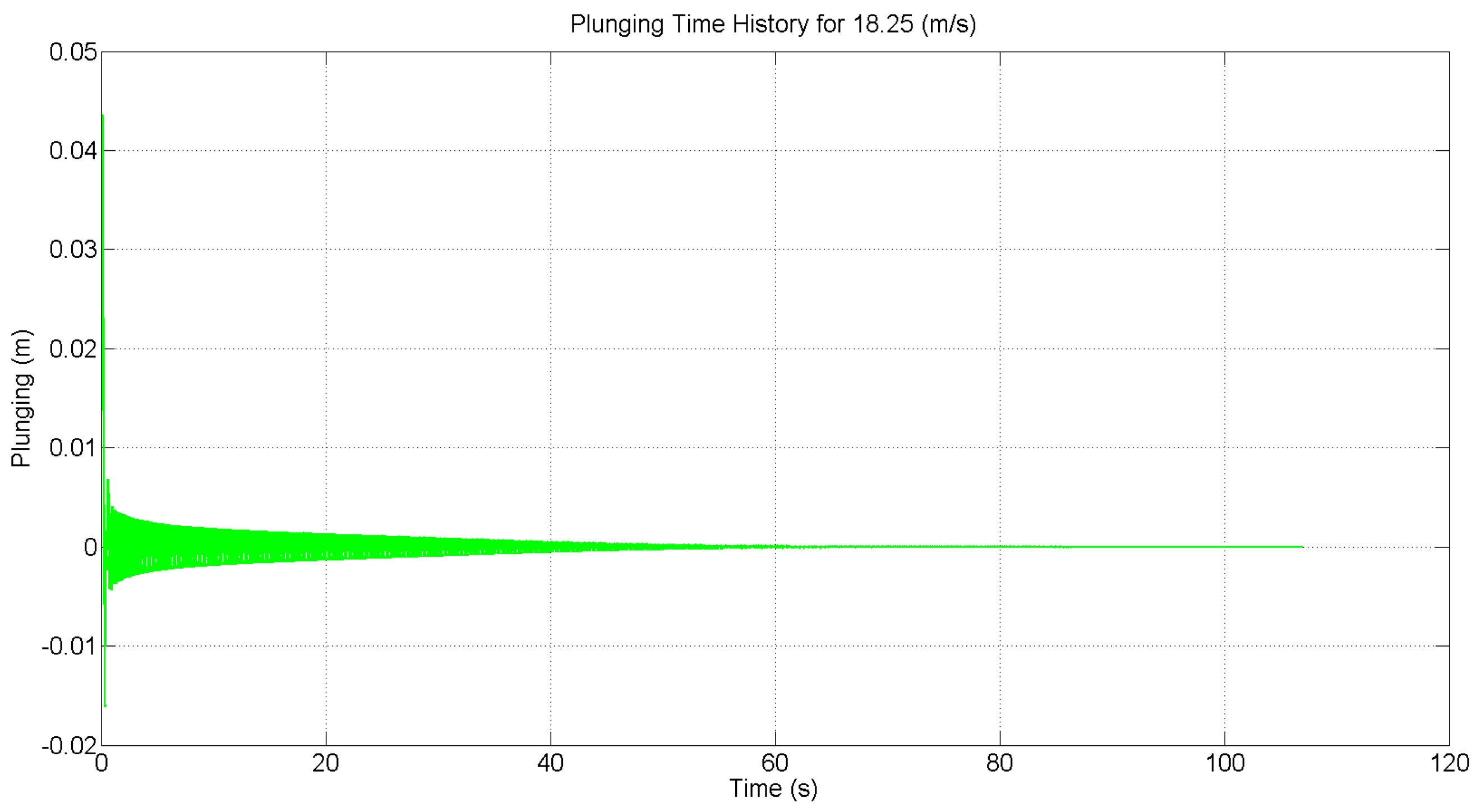
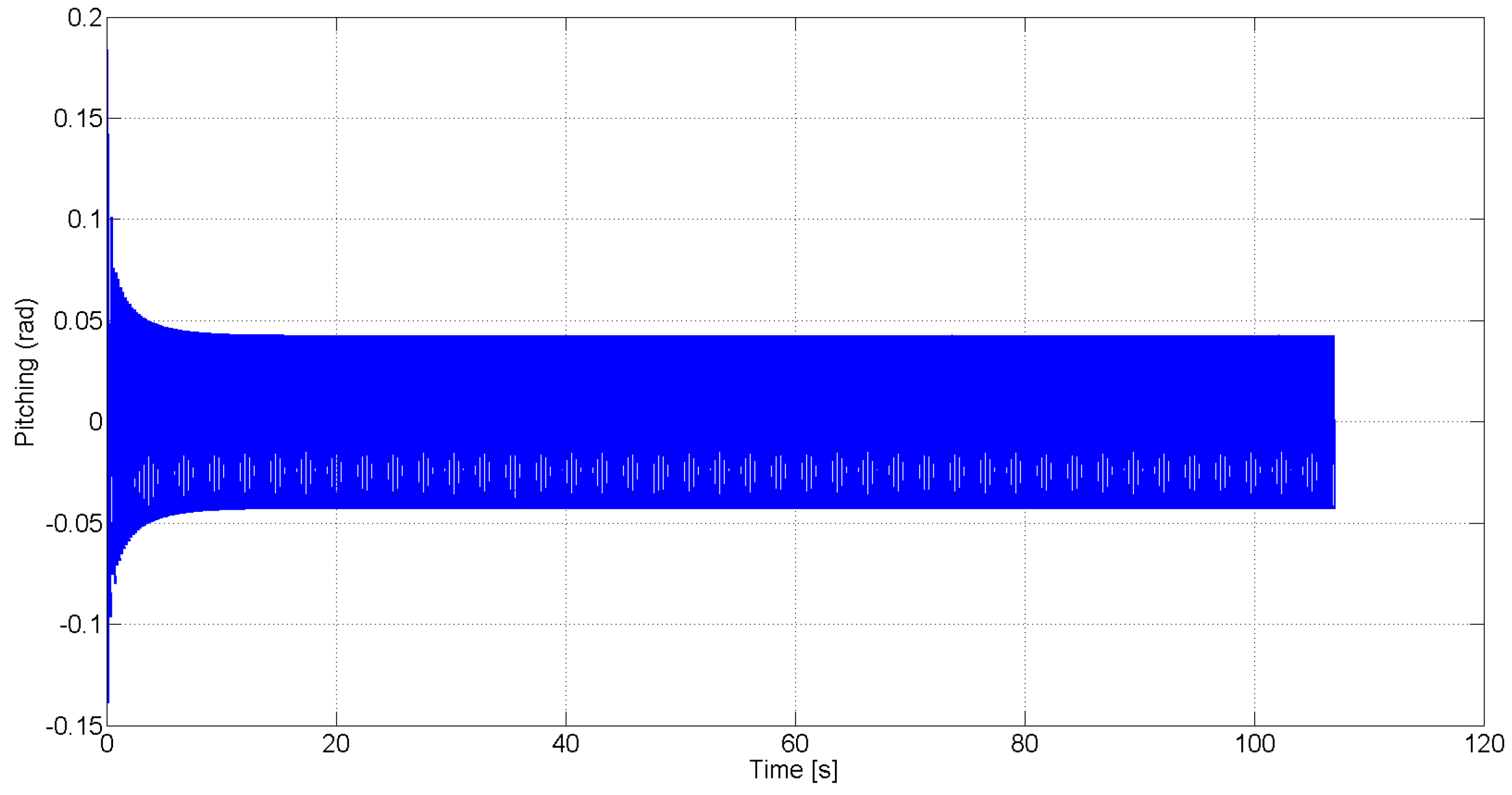
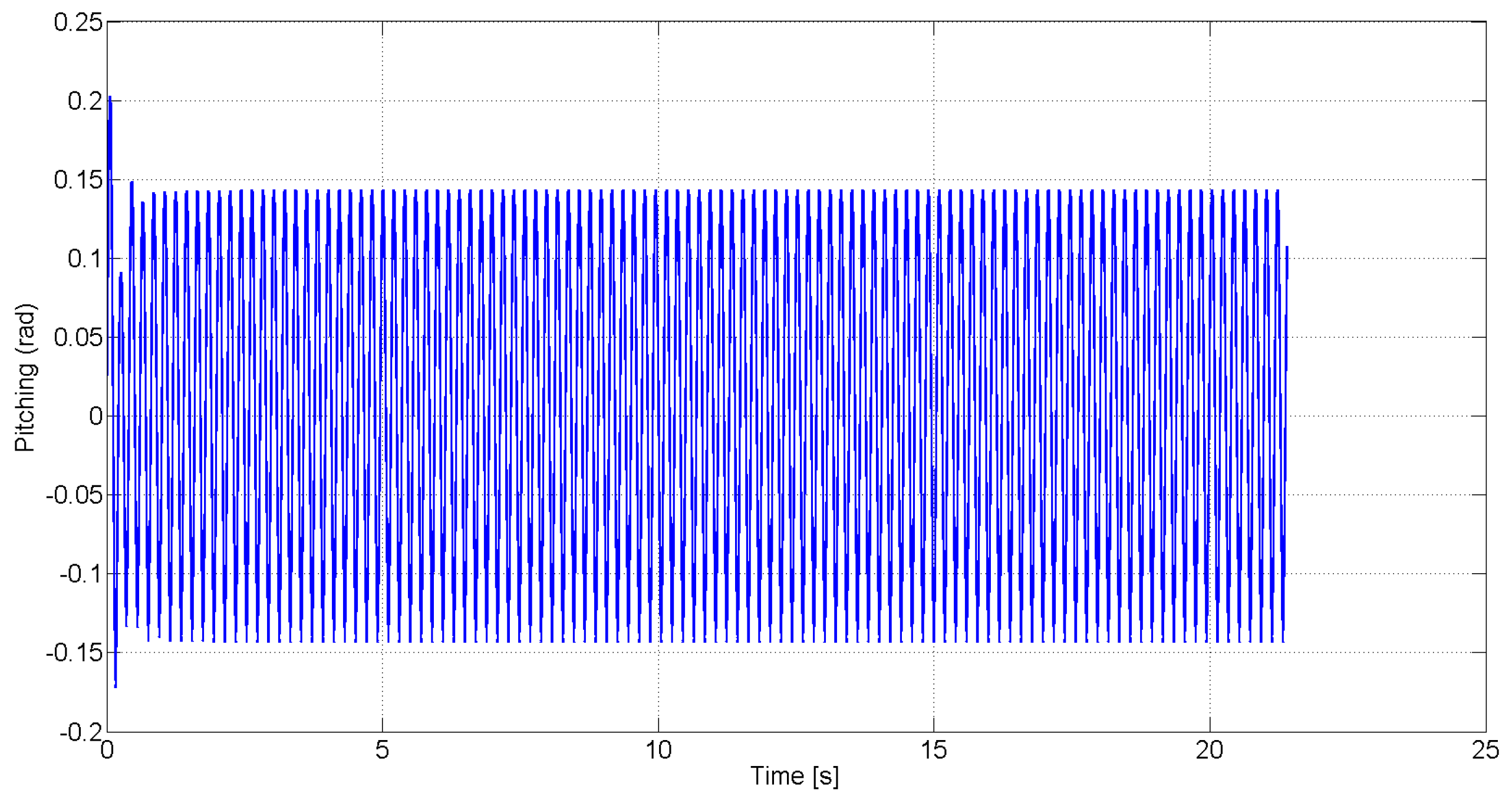
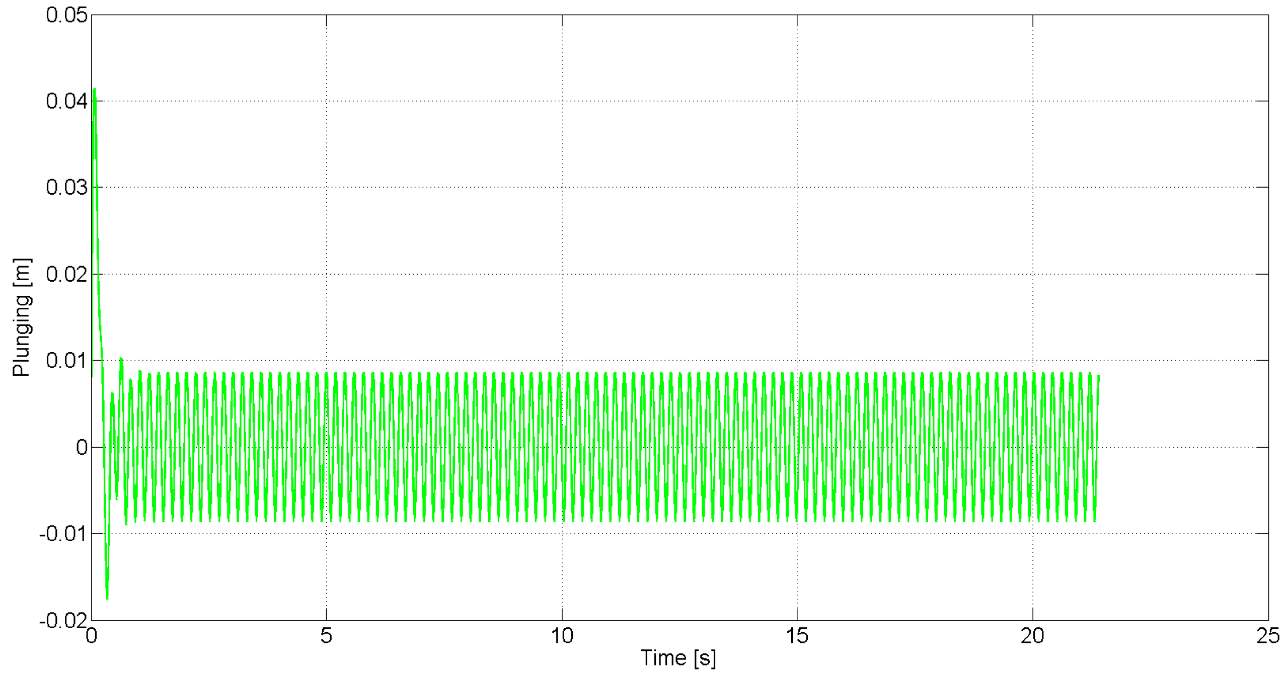
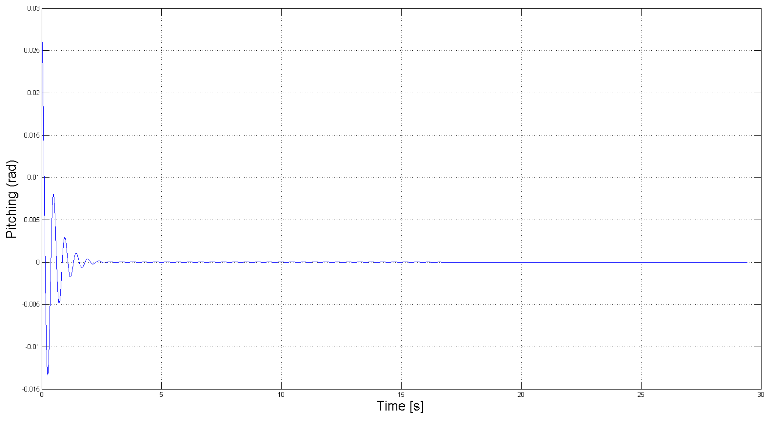
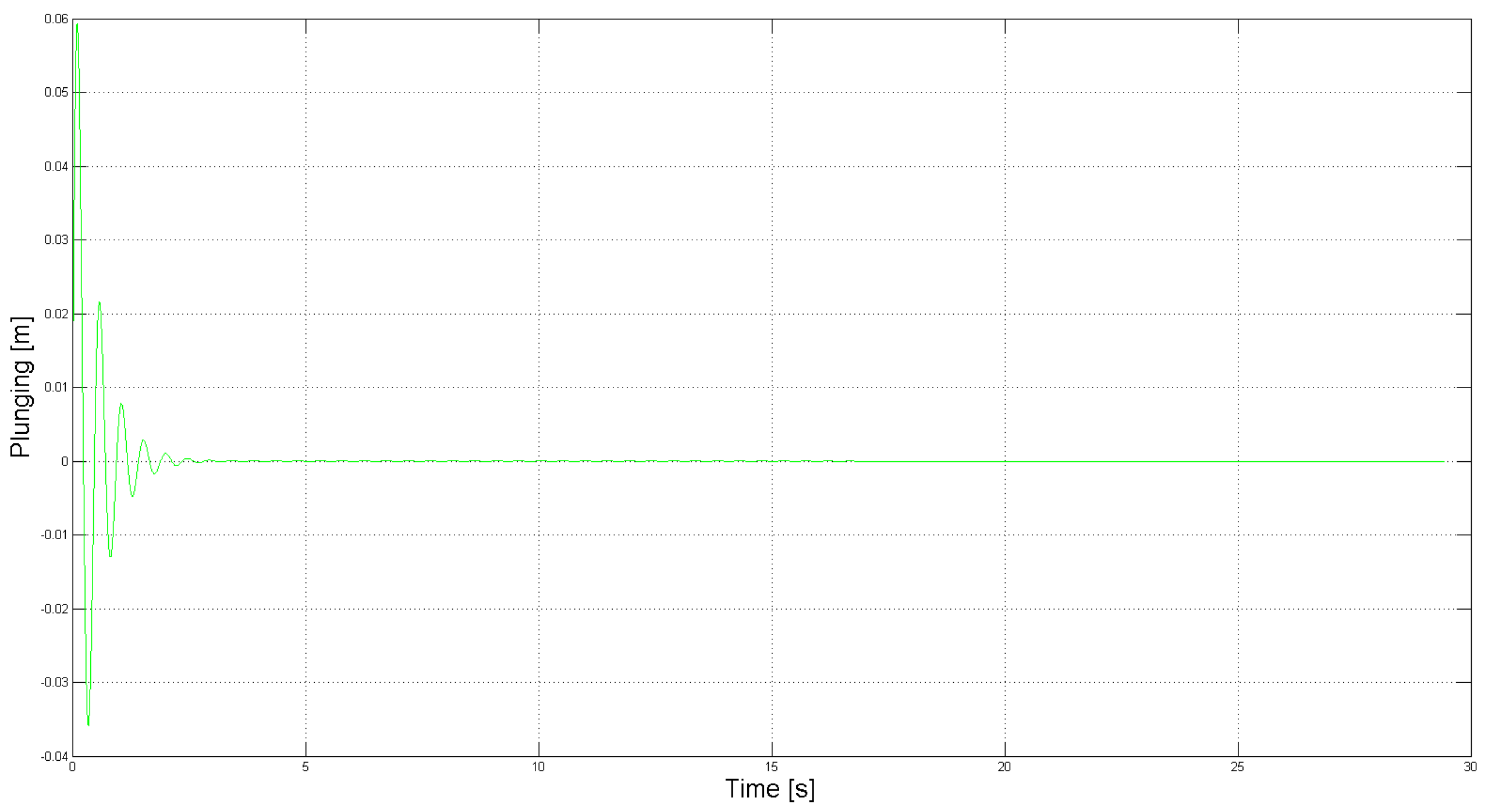
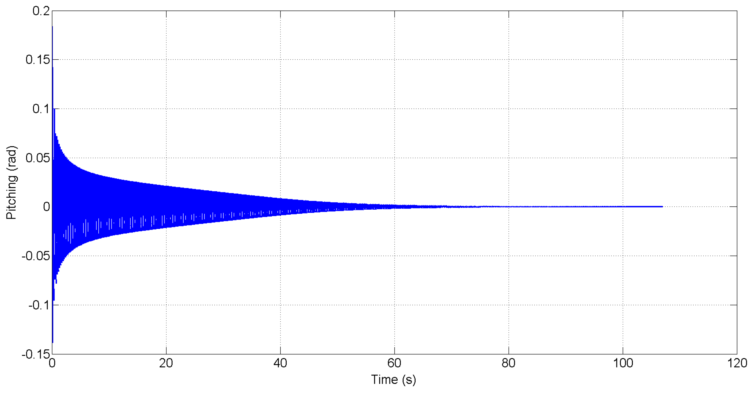
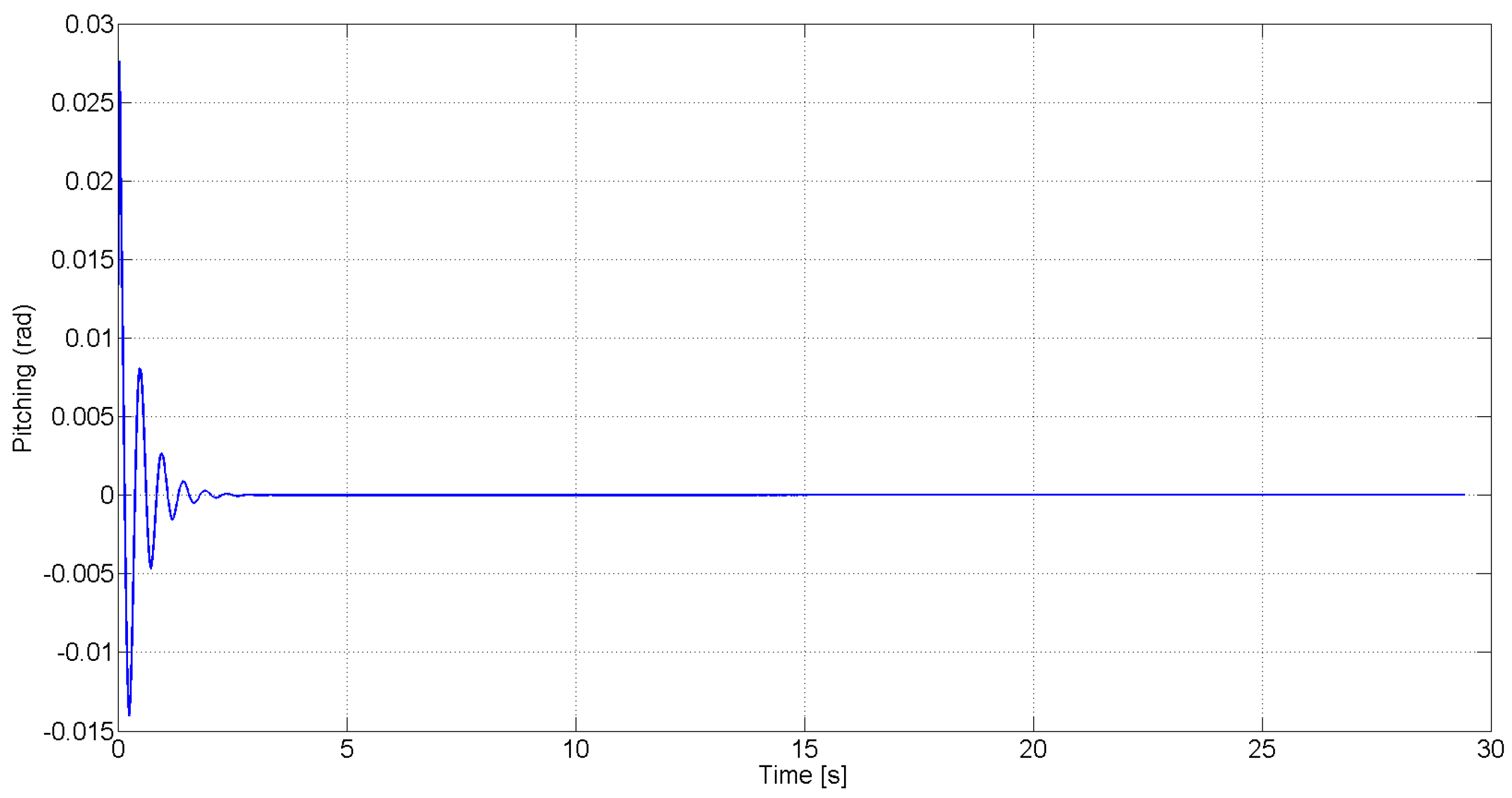
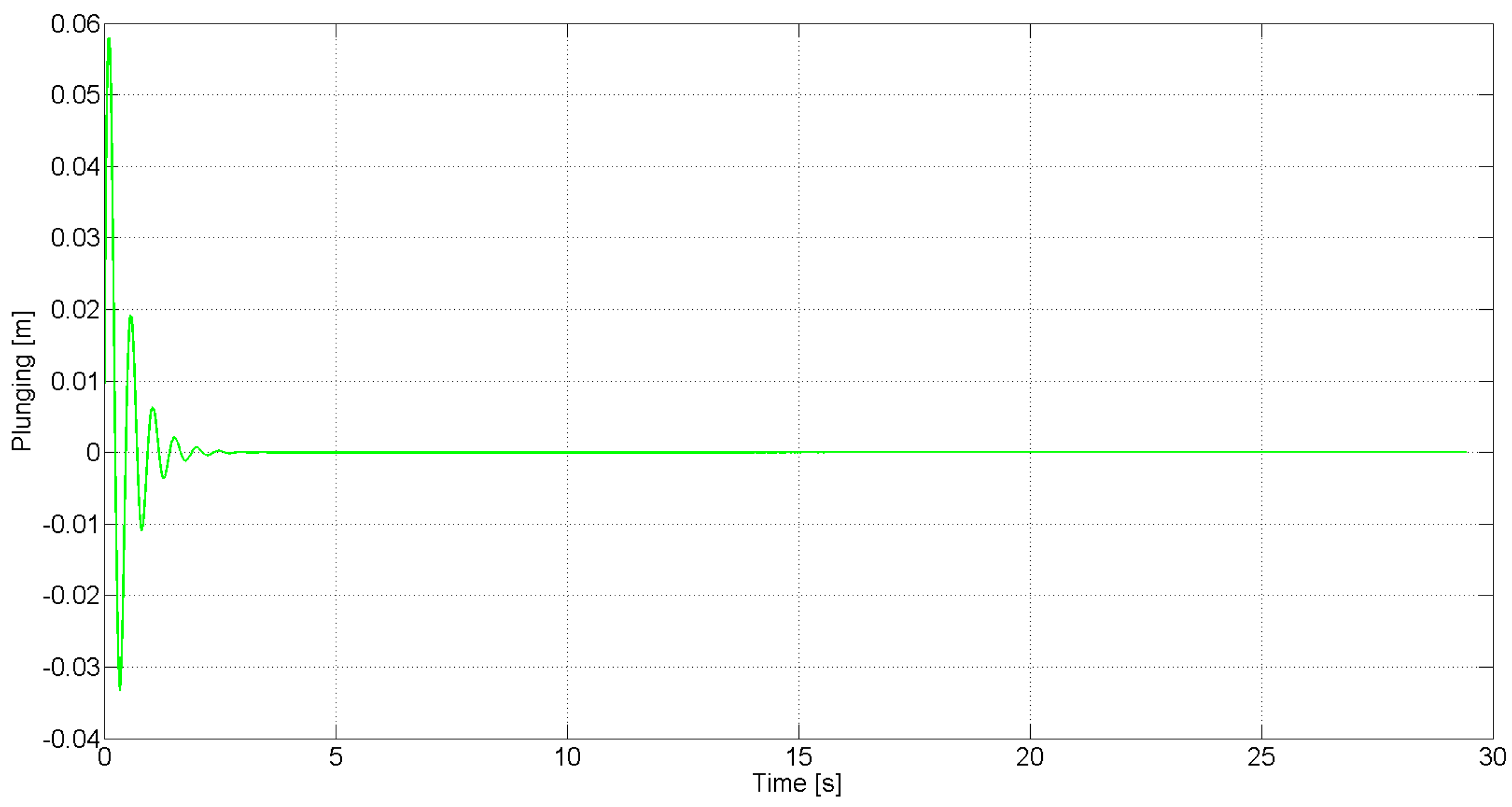
Figure 2, Figure 3 and Figure 4, Figure 5 show the open-loop pitching and plunging response of the simulated system for the case where the free stream velocity U is 18.25 $m/s$ and 19.5 $m/s$, respectively. These figures demonstrate that sustained LCO occur in the absence of feedback control. 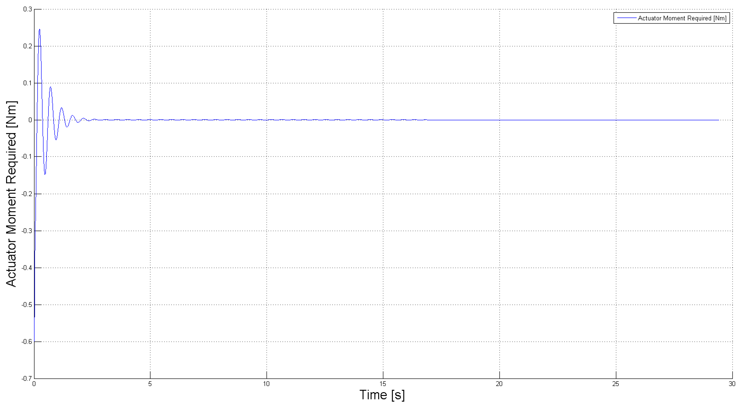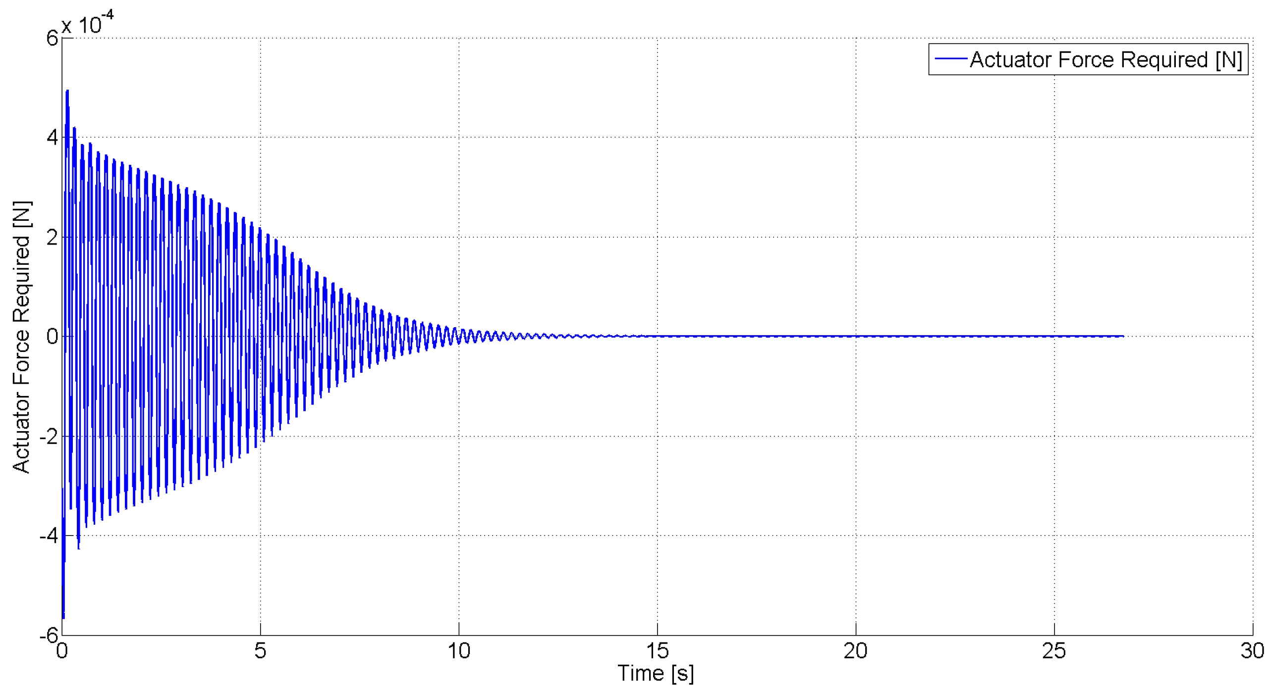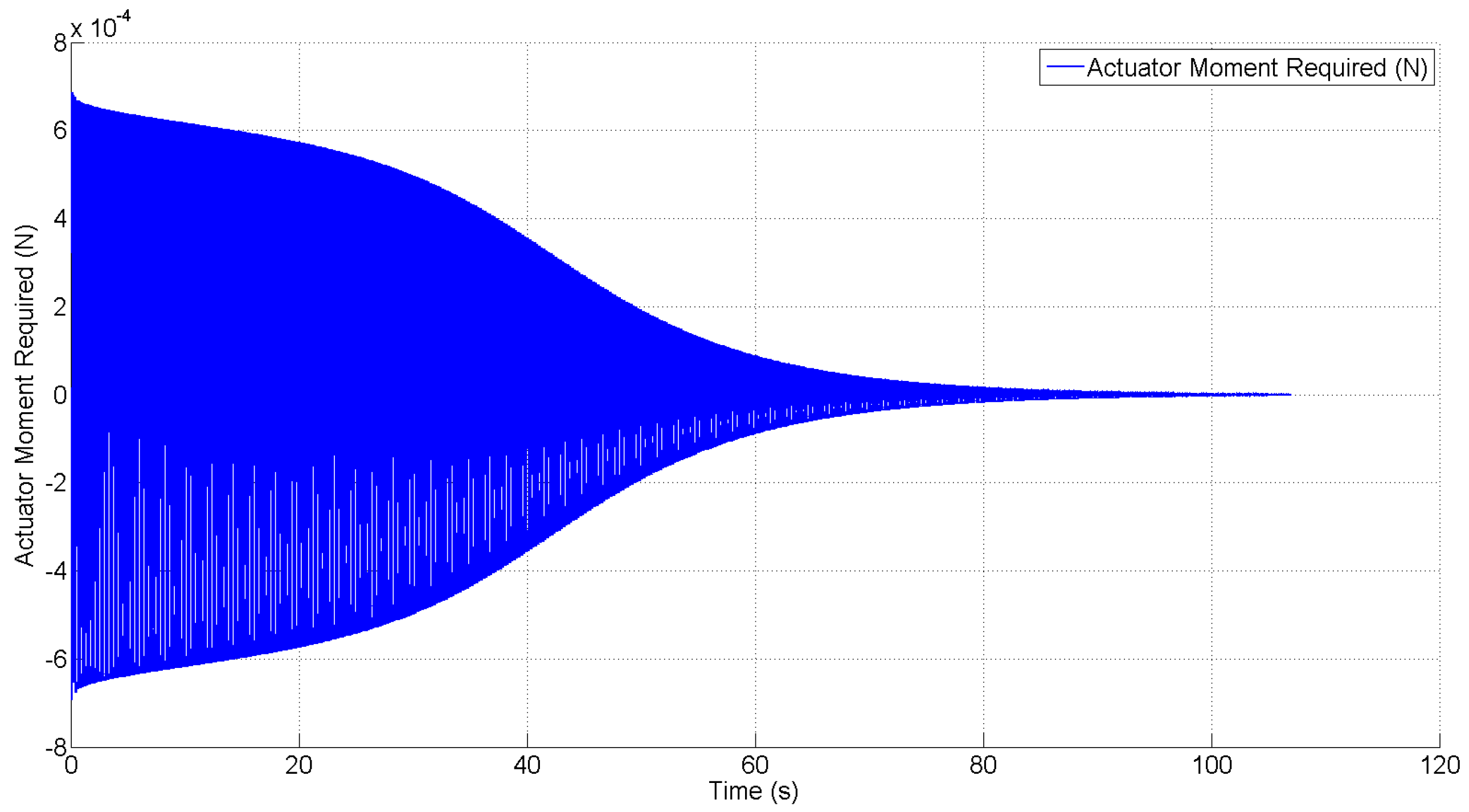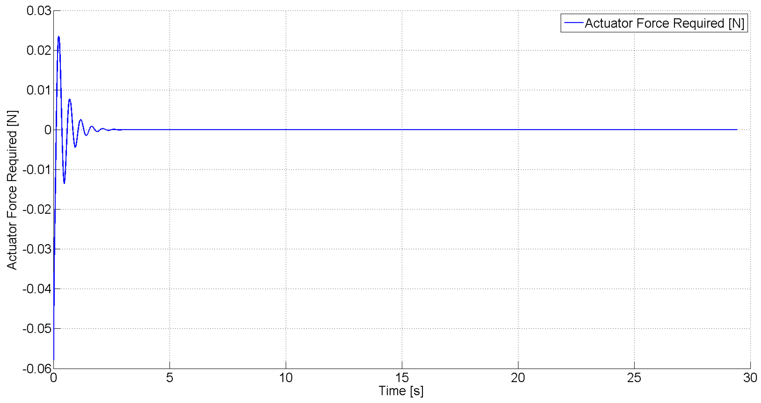Figure 6 and Figure 7 show the closed-loop pitching and plunging response for the case where $U=18.25$ $m/s$, and Figure 8 and Figure 9 show the required control force and moment, respectively, in this case. These simulation results demonstrate the capability of the robust control law to asymptotically suppress LCO using a control force and moment that are within reasonable limits. This demonstrates the practical efficacy of the control design to suppress LCO using the limited control authority that is available from the SJA. It should be noted, however, that in actual application, arrays consisting of several SJAs can be utilized to realize a greater overall control force and moment.

Figure 2. Uncontrolled pitching response for free stream velocity $U=18.25$ $m/s$.

Figure 2. Uncontrolled pitching response for free stream velocity $U=18.25$ $m/s$.

Figure 3. Uncontrolled plunging response for free stream velocity $U=18.25$ $m/s$.

Figure 3. Uncontrolled plunging response for free stream velocity $U=18.25$ $m/s$.

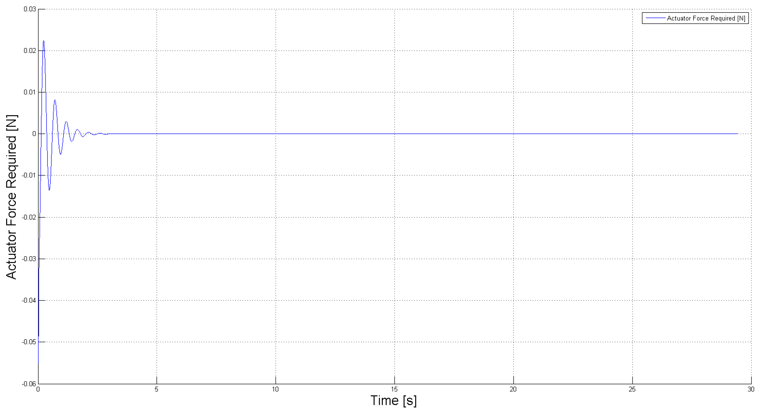
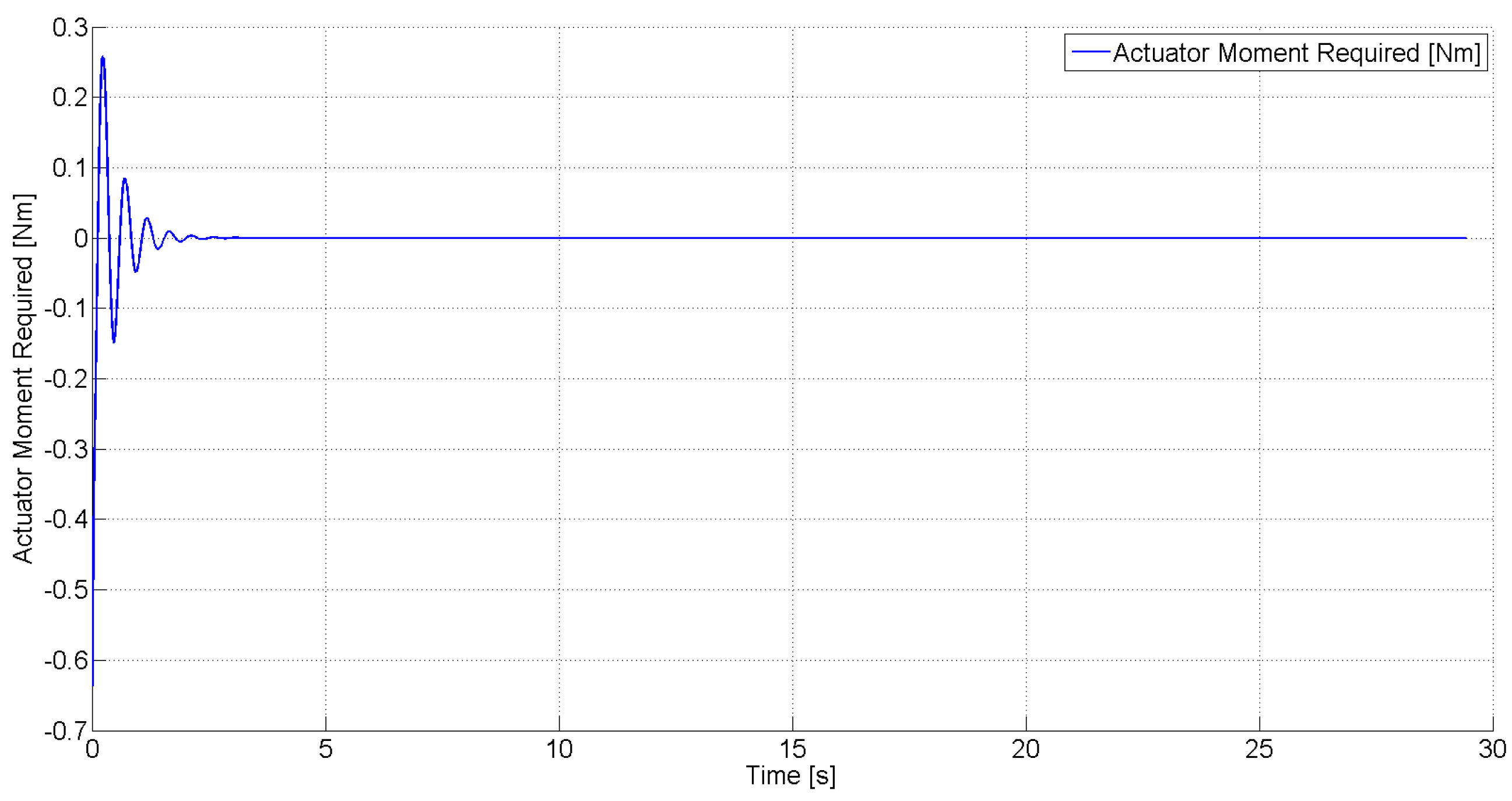
Figure 10, Figure 11 and Figure 12, Figure 13 show the closed-loop pitching and plunging response and the required control force and moment, respectively, for the case where the free stream velocity $U=19.5m/s$. Figure 14, Figure 15 and Figure 16, Figure 17 show the closed-loop pitching and plunging response and the required control moment and force for the case where $U=20.5m/s$. As shown in the figures, an increased control effort is required to suppress the LCO in the presence of the increased air velocity.

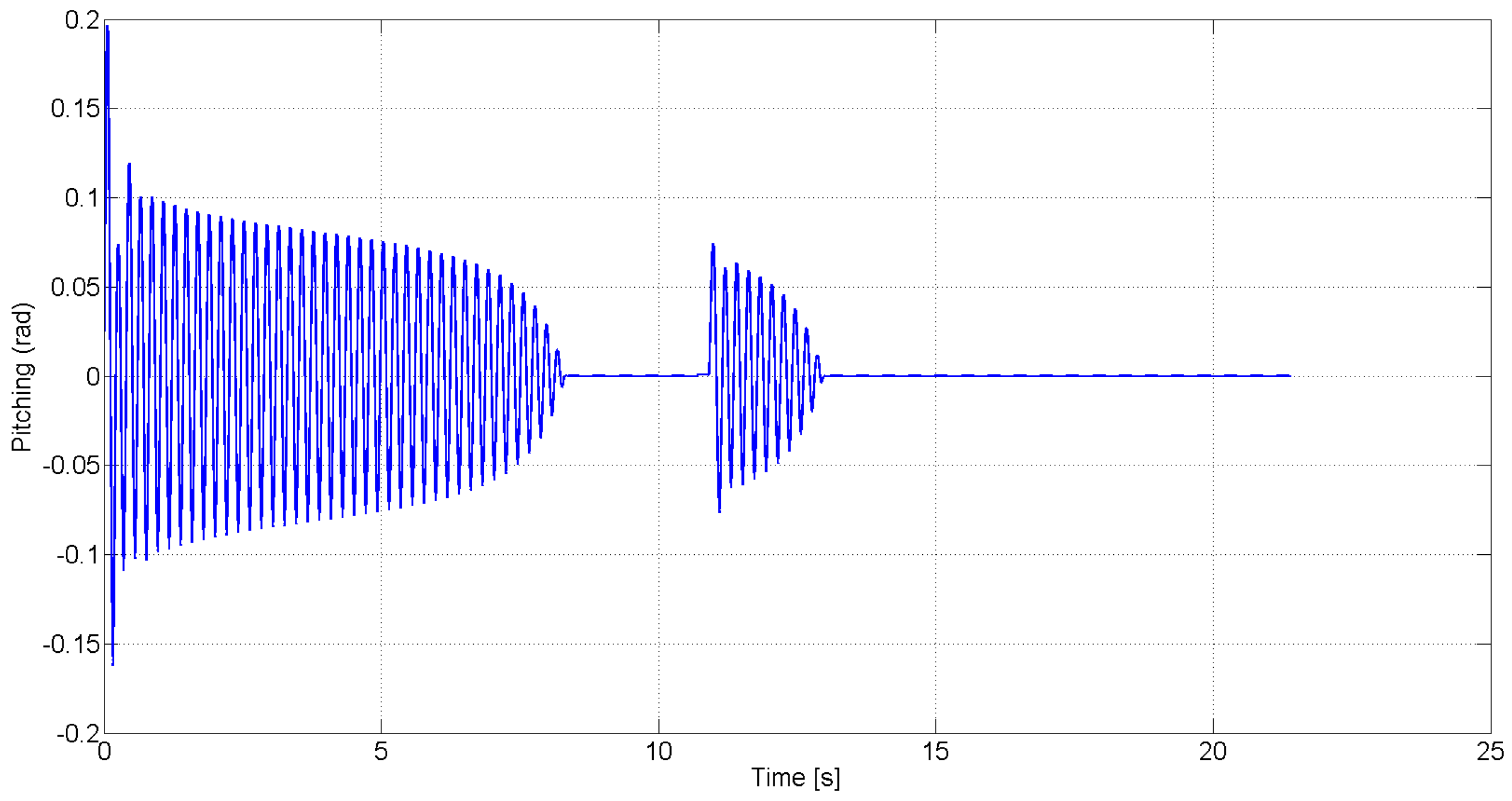
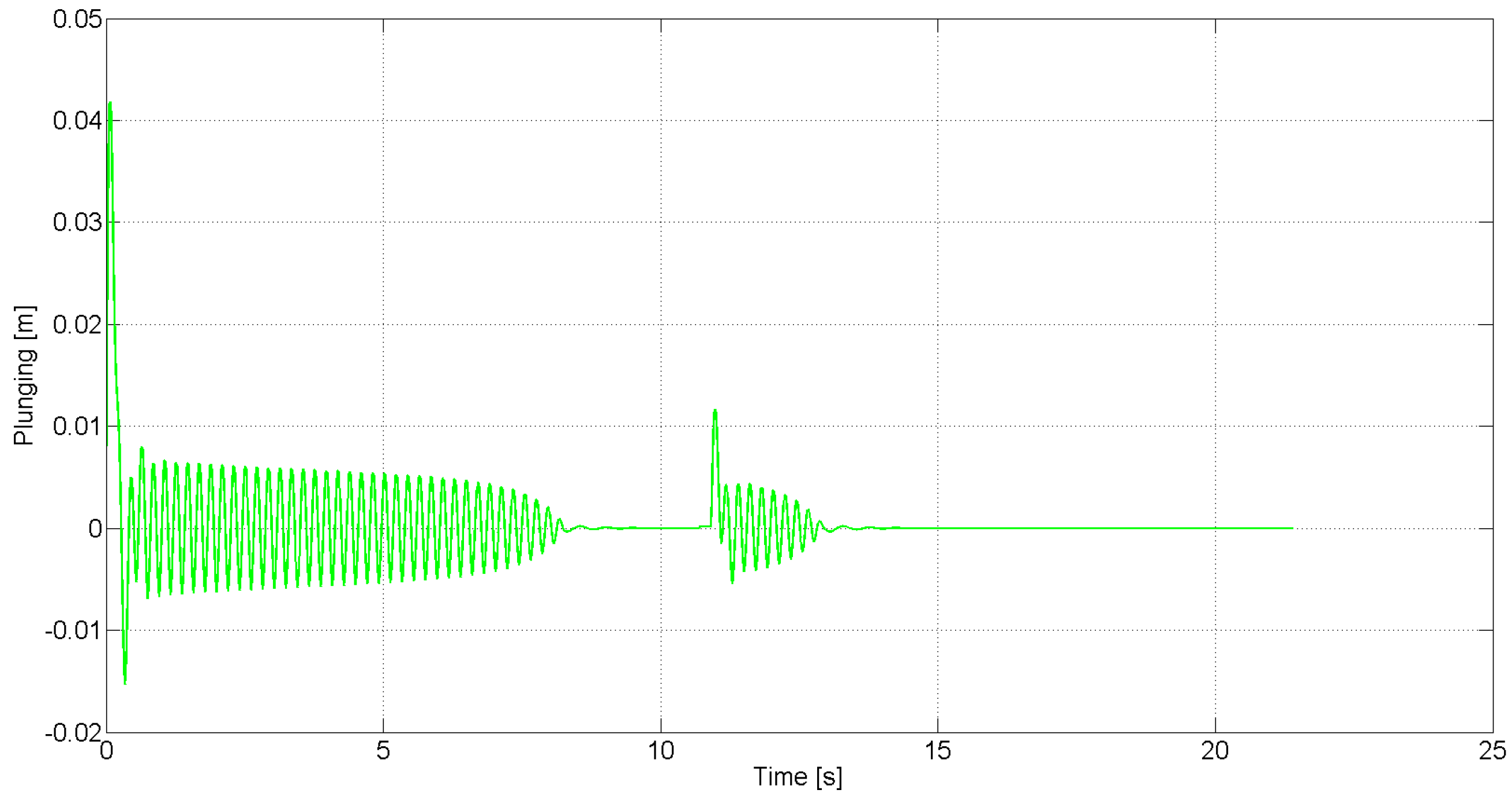
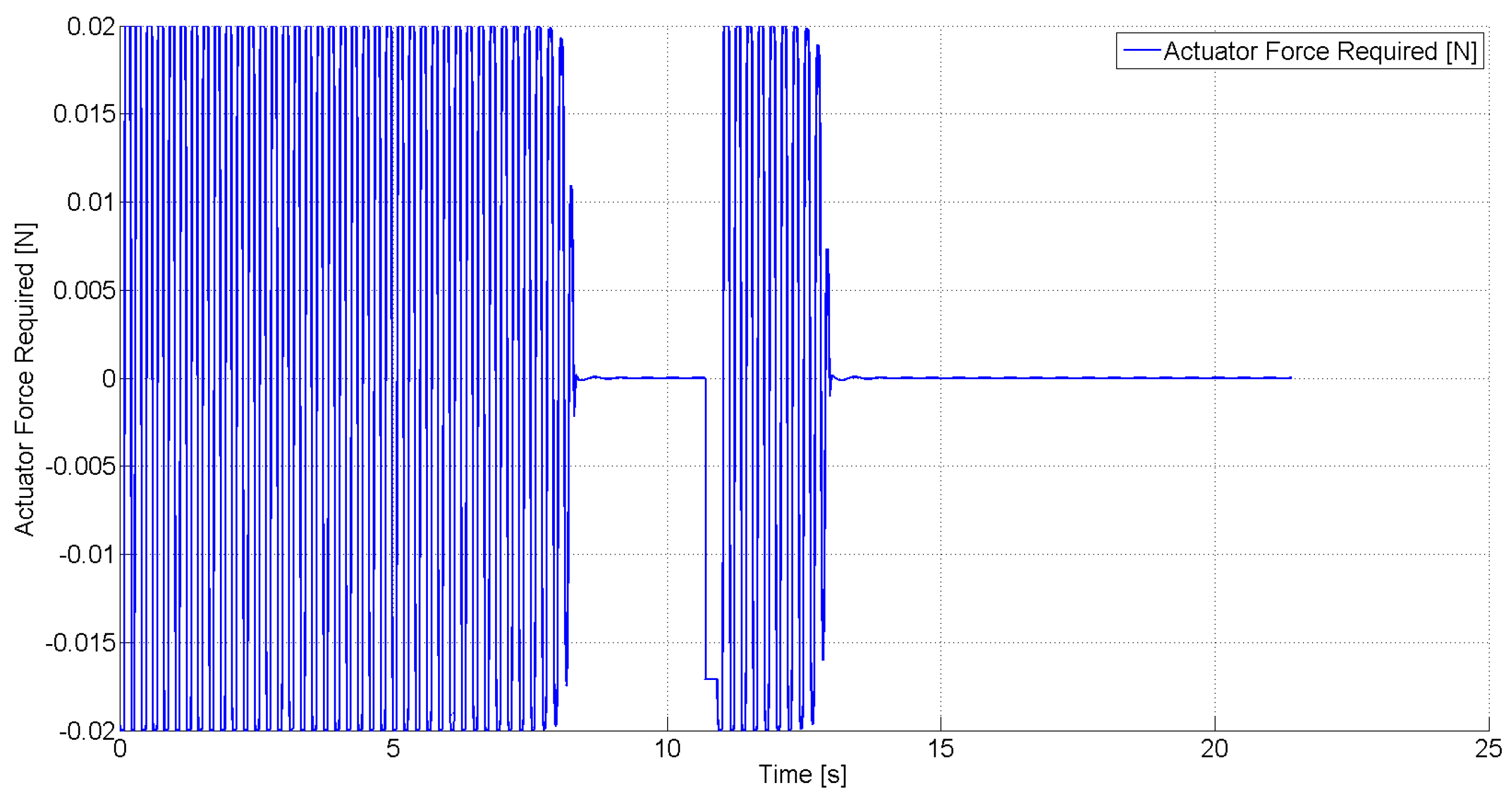
Figure 18 and Figure 19 show the robustness of the proposed controller in the event of sudden unmodeled disturbances. In these plots, a sudden increase (i.e., step function) in the pitching and plunging rates was programmed to occur at $10.9s$. Simultaneously, the free stream velocity U was increased from $19m/s$ to $25m/s$ for approximately 0.2 seconds to simulate a disturbance due to a wind gust. The pitching and plunging responses in Figure 18 and Figure 19 demonstrate the capability of the control law to compensate for the sudden and unexpected disturbances. 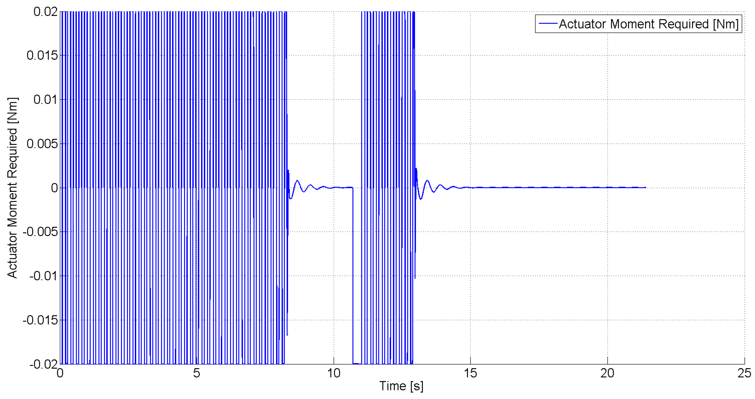Figure 20 and Figure 21 show the commanded control force and moment, respectively, of the closed-loop system in response to the disturbance.

Figure 4. Uncontrolled pitching response for free stream velocity $U=19.5$ $m/s$.

Figure 4. Uncontrolled pitching response for free stream velocity $U=19.5$ $m/s$.

Figure 5. Uncontrolled plunging response for free stream velocity $U=19.5$ $m/s$.

Figure 5. Uncontrolled plunging response for free stream velocity $U=19.5$ $m/s$.

Figure 6. Closed-loop pitching response for free stream velocity $U=18.25$ $m/s$.

Figure 6. Closed-loop pitching response for free stream velocity $U=18.25$ $m/s$.

Figure 7. Closed-loop plunging response for free stream velocity $U=18.25$ $m/s$.

Figure 7. Closed-loop plunging response for free stream velocity $U=18.25$ $m/s$.

Figure 8. Actuator force required for free stream velocity $U=18.25$ $m/s$.

Figure 8. Actuator force required for free stream velocity $U=18.25$ $m/s$.

Figure 9. Actuator moment required for free stream velocity $U=18.25$ $m/s$.

Figure 9. Actuator moment required for free stream velocity $U=18.25$ $m/s$.

Figure 10. Closed-loop pitching response for free stream velocity $U=19.5$ $m/s$.

Figure 10. Closed-loop pitching response for free stream velocity $U=19.5$ $m/s$.

Figure 11. Closed-loop plunging response required for free stream velocity $U=19.5$ $m/s$.

Figure 11. Closed-loop plunging response required for free stream velocity $U=19.5$ $m/s$.

Figure 12. Actuator force required for free stream velocity $U=19.5$ $m/s$.

Figure 12. Actuator force required for free stream velocity $U=19.5$ $m/s$.

Figure 13. Actuator moment required for free stream velocity $U=19.5$ $m/s$.

Figure 13. Actuator moment required for free stream velocity $U=19.5$ $m/s$.

Figure 14. Closed-loop pitching response for free stream velocity $U=20.5$ $m/s$.

Figure 14. Closed-loop pitching response for free stream velocity $U=20.5$ $m/s$.

Figure 15. Closed-loop plunging response for free stream velocity $U=20.5$ $m/s$.

Figure 15. Closed-loop plunging response for free stream velocity $U=20.5$ $m/s$.

Figure 16. Actuator force required for free stream velocity $U=20.5$ $m/s$.

Figure 16. Actuator force required for free stream velocity $U=20.5$ $m/s$.

Figure 17. Actuator moment required for free stream velocity $U=20.5$ $m/s$.

Figure 17. Actuator moment required for free stream velocity $U=20.5$ $m/s$.

Figure 18. Closed-loop pitching response in the presence of a disturbance.

Figure 18. Closed-loop pitching response in the presence of a disturbance.

Figure 19. Closed-loop plunging response in the presence of a disturbance.

Figure 19. Closed-loop plunging response in the presence of a disturbance.

Figure 20. Actuator force use in the presence of a disturbance.

Figure 20. Actuator force use in the presence of a disturbance.

Figure 21. Actuator moment response in the presence of a disturbance.

Figure 21. Actuator moment response in the presence of a disturbance.

5. Conclusions

A nonlinear robust control law for SJA-based LCO suppression in UAV wings is presented. The proposed control law is rigorously proven to achieve global asymptotic regulation of the pitching and plunging displacements to zero in the presence of dynamic model uncertainty and parametric actuator uncertainty. Furthermore, the proposed control law is shown via numerical simulation to compensate for unmodeled external disturbances (i.e., due to wind gusts and unmodeled effects). It is further shown that the robust control law can achieve suppression of LCO using minimal control effort. Future work will address LCO suppression control design, which can be proven to achieve simultaneous pitching and plunging regulation using only a scalar control input (i.e., the underactuated control problem). In addition, future work will target controller validation via high-fidelity computational fluid dynamics simulations.