Parametric Calculations of Radiative Decay Rates for Magnetic Dipole and Electric Quadrupole Transitions in Tm IV, Yb V, and Er IV

Abstract
:1. Introduction
2. Experimental and Theoretical Methods
3. Results and Discussion
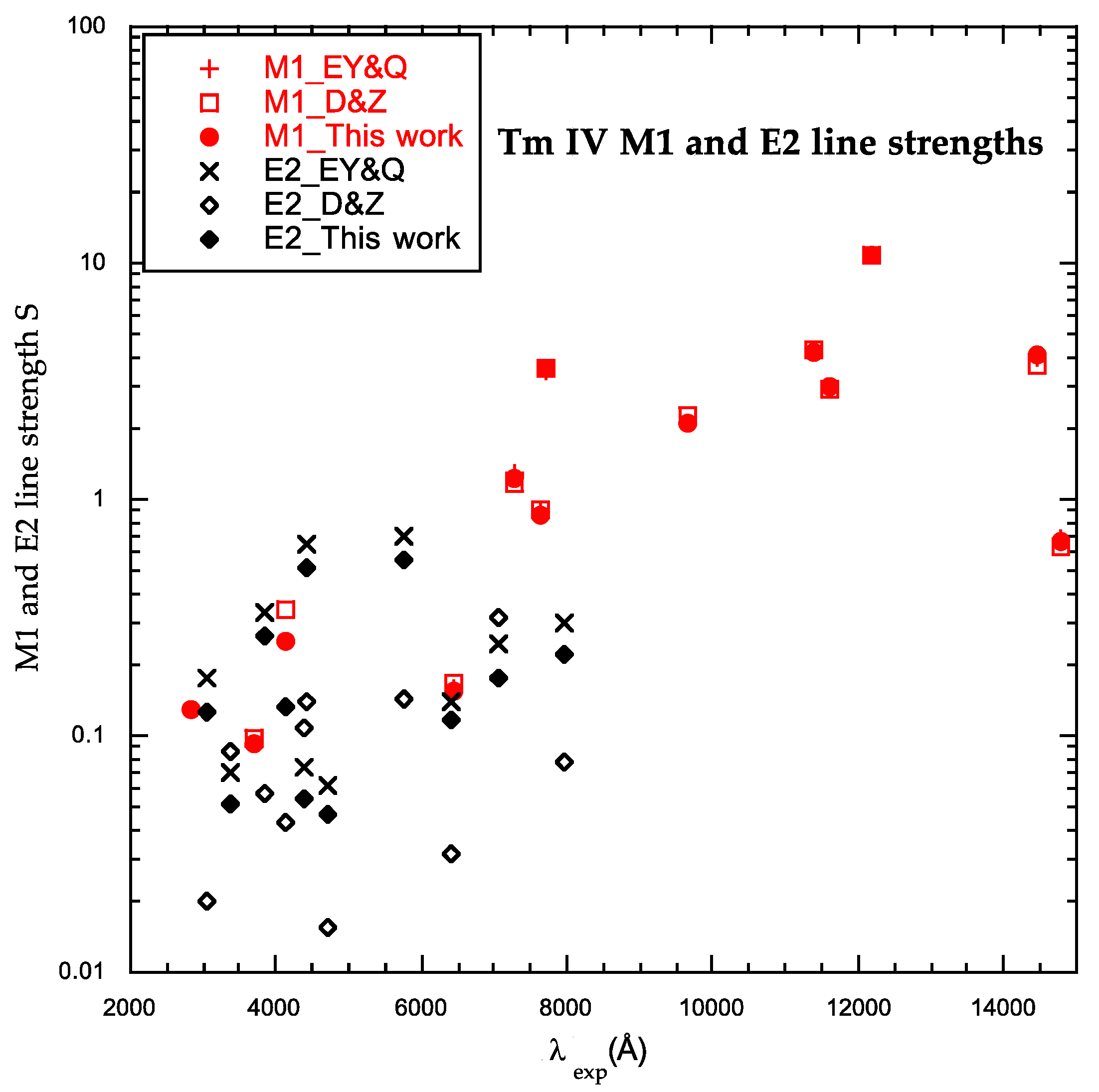
3.1. Tm IV
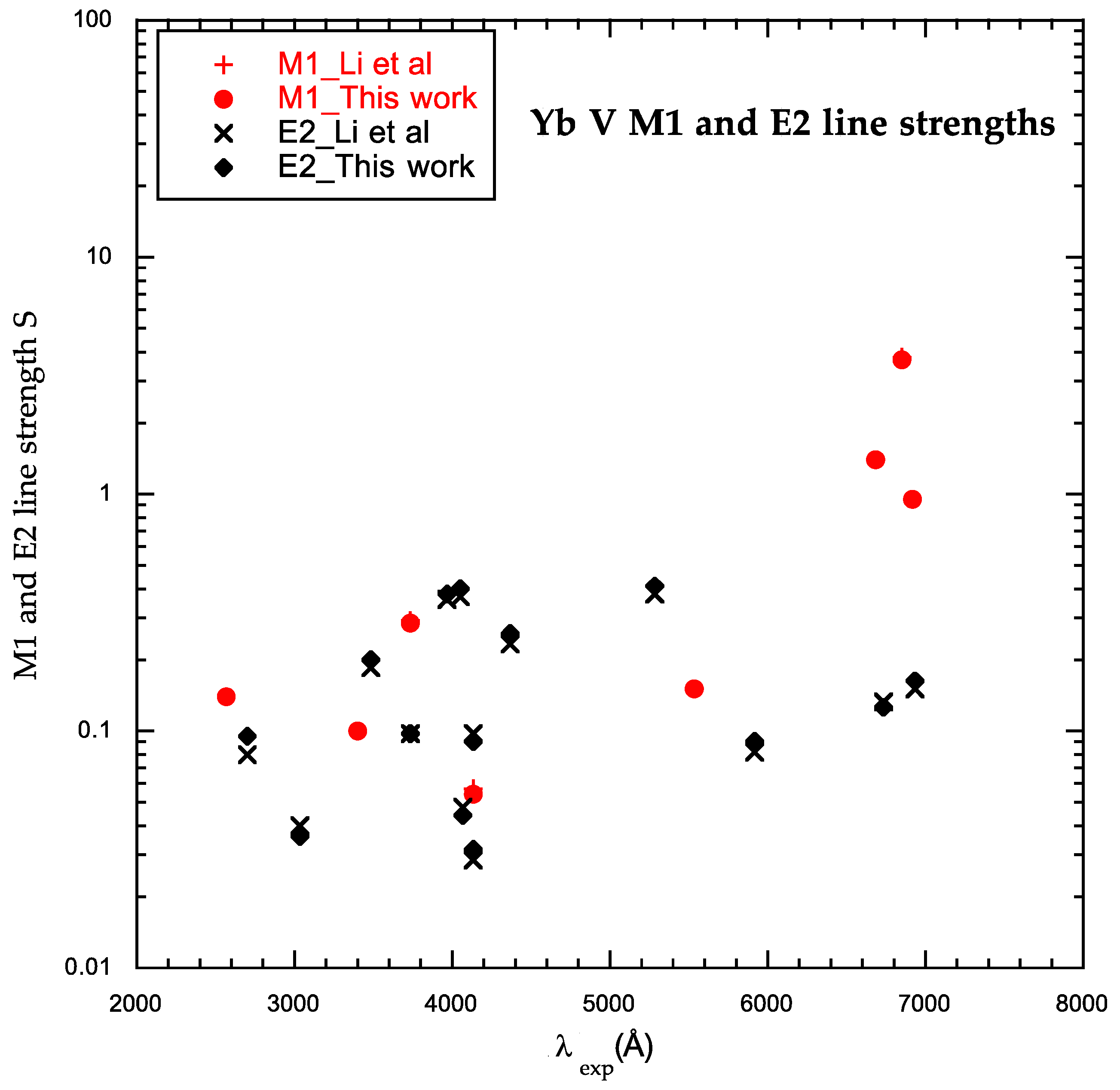
3.2. Yb V
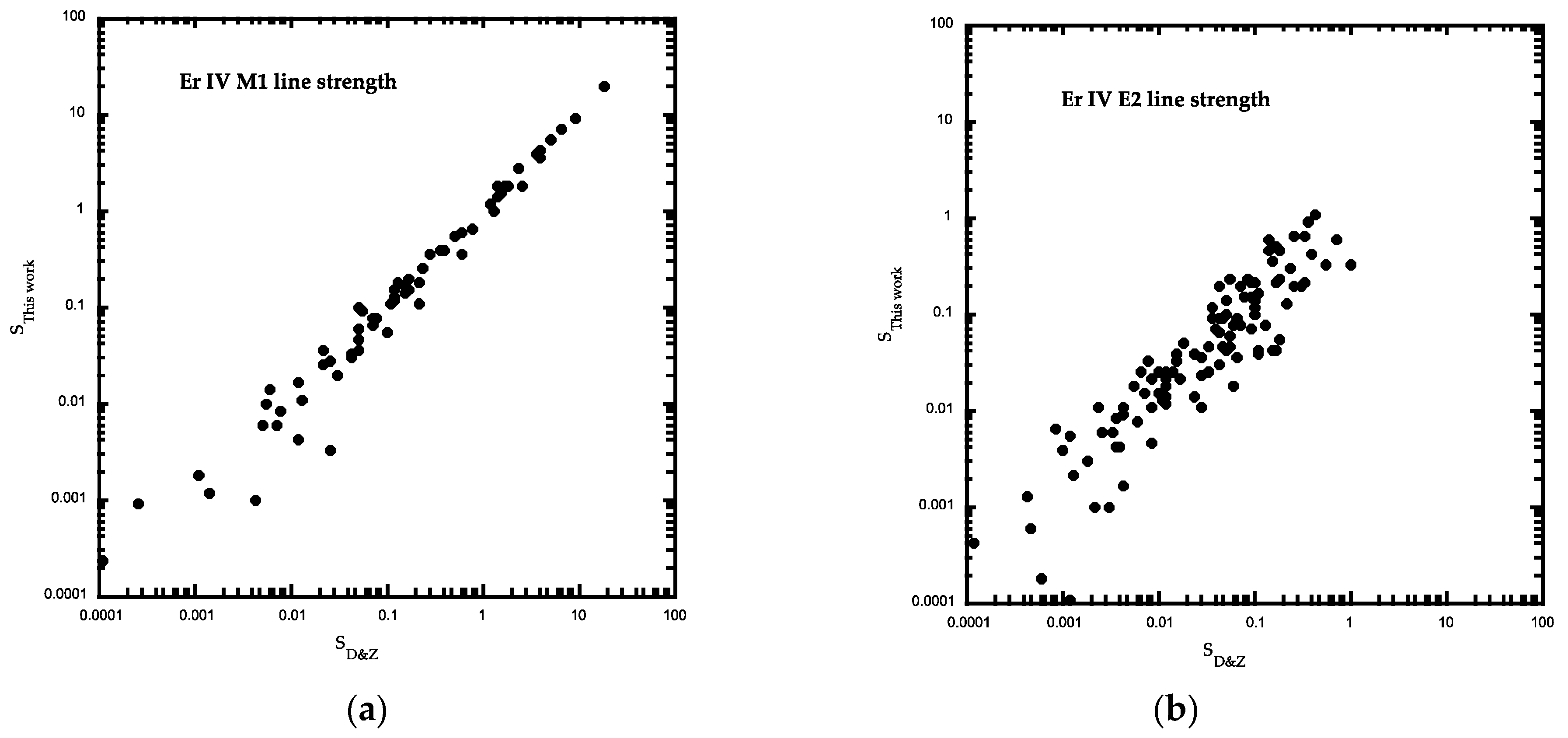
3.3. Er IV
3.4. Scaling Factors of Energy Parameters as Derived from Least-Squares Fits
4. Conclusions
Author Contributions
Funding
Acknowledgments
Conflicts of Interest
References
- Wybourne, B.G. The fascination of the rare earths—Then, now and in the future. J. Alloys Compd. 2004, 380, 96–100. [Google Scholar] [CrossRef]
- Carnall, W.T.; Fields, P.R.; Wybourne, B.G. Spectral intensities of the trivalent lanthanides and actinides in solution. I. Pr3+, Nd3+, Er3+, Tm3+, and Yb3+. J. Chem. Phys. 1965, 42, 3797–3806. [Google Scholar] [CrossRef]
- Carnall, W.T.; Fields, P.R.; Wybourne, B.G. Spectral intensities of the trivalent lanthanides and actinides in solution. II. Pm3+, Sm3+, Eu3+, Gd3+, Tb3+, Dy3+, and Ho3+. J. Chem. Phys. 1968, 49, 4412–4423. [Google Scholar] [CrossRef]
- Ryabchikova, T.; Ryabtsev, A.N.; Kochukov, O.; Bagnulo, S. Rare-earth elements in the atmosphere of the magnetic chemically peculiar star HD 144897. New classification of the Nd III spectrum. Astron. Astrophys. 2006, 456, 329–338. [Google Scholar] [CrossRef]
- Kasen, D.; Badnell, N.R.; Barnes, J. Opacities and spectra of the r-process ejecta from neutron star mergers. Astrophys. J. 2013, 774, 25. [Google Scholar] [CrossRef]
- Fontes, C.J.; Fryer, C.L.; Hungerford, A.L.; Hakel, P.; Colgan, J.; Kilcrease, D.P.; Sherrill, M.E. Relativistic opacities for astrophysical applications. High Energy Density Phys. 2015, 16, 53–59. [Google Scholar] [CrossRef] [Green Version]
- Wyart, J.-F.; Meftah, A.; Bachelier, A.; Sinzelle, J.; Tchang-Brillet, W.-Ü.L.; Champion, N.; Spector, N.; Sugar, J. Energy levels of 4f3 in the Nd3+ free ion from emission spectra. J. Phys. B Mol. Opt. Phys. 2006, 39, L77. [Google Scholar] [CrossRef]
- Wyart, J.-F.; Meftah, A.; Tchang-Brillet, W.-Ü.L.; Champion, N.; Lamrous, O.; Spector, N.; Sugar, J. Analysis of the free ion Nd3+ spectrum (Nd IV). J. Phys. B At. Mol. Opt. Phys. 2007, 40, 3957–3972. [Google Scholar] [CrossRef]
- Wyart, J.-F.; Meftah, A.; Sinzelle, J.; Tchang-Brillet, W.-Ü.L.; Spector, N.; Judd, B. Theoretical study of ground-state configurations 4fN in Nd IV, Pr IV and Nd V. J. Phys. B At. Mol. Opt. Phys. 2008, 41, 085001. [Google Scholar] [CrossRef]
- Wyart, J.-F.; Meftah, A.; Sinzelle, J.; Tchang-Brillet, W.-Ü.L.; Champion, N.; Spector, N.; Sugar, J. Spectrum and energy levels of the Nd4+ free ion (Nd V). Phys. Scr. 2008, 77, 055302. [Google Scholar]
- Meftah, A.; Wyart, J.-F.; Champion, N.; Tchang-Brillet, W.-Ü.L. Observation and interpretation of the Tm3+ free ion spectrum. Eur. Phys. J. D 2007, 44, 35–45. [Google Scholar] [CrossRef]
- Meftah, A.; Wyart, J.-F.; Tchang-Brillet, W.-Ü.L.; Blaess, C.; Champion, N. Spectrum and energy levels of the Yb4+ free ion (Yb V). Phys. Scr. 2013, 88, 045305. [Google Scholar] [CrossRef]
- Deghiche, D.; Meftah, A.; Wyart, J.-F.; Champion, N.; Blaess, C.; Tchang-Brillet, W.-Ü.L. Observation of core-excited configuration in four-time ionized neodymium Nd4+ (Nd V). Phys. Scr. 2015, 90, 095402. [Google Scholar] [CrossRef]
- Meftah, A.; Ait Mammar, S.; Wyart, J.-F.; Tchang-Brillet, W.-Ü.L.; Champion, N.; Blaess, C.; Deghiche, D.; Lamrous, O. Analysis of the free ion spectrum of Er3+ (Er IV). J. Phys. B At. Mol. Opt. Phys. 2016, 49, 165002. [Google Scholar] [CrossRef]
- Cowan, R.D. The Theory of Atomic Structure and Spectra; University of California Press: Berkeley, CA, USA, 1981. [Google Scholar]
- Kramida, A. A Suite of Atomic Structure Codes Originally Developed by R. D. Cowan Adapted for Windows-Based Personal Computers. Available online: http://das101.isan.troitsk.ru/COWAN (accessed on 5 May 2017).
- Judd, B.R. Optical absorption intensities of rare-earth ions. Phys. Rev. 1962, 127, 750–761. [Google Scholar] [CrossRef]
- Ofelt, G.S. Intensities of crystal spectra of rare-earth ions. J. Chem. Phys. 1962, 37, 511–520. [Google Scholar] [CrossRef]
- Dodson, C.M.; Zia, R. Magnetic dipole and electric quadrupole transitions in the trivalent lanthanide series: Calculated emission rates and oscillator strengths. Phys. Rev. B 2012, 86, 126102. [Google Scholar] [CrossRef]
- Enzonga Yoca, S.; Quinet, P. Radiative decay rates for electric dipole, magnetic dipole and electric quadrupole transitions in triply ionized Thulium (Tm IV). Atoms 2017, 5, 28. [Google Scholar] [CrossRef]
- Li, H.; Kuang, X.-Y.; Yeung, Y.Y. Semi-empirical calculations of radiative rates for parity-forbidden transitions within the 4f2 configuration of Ba-like ions La+, Ce2+, Pr3+ and Nd4+ and 4f12 configuration of Dy-like Yb4+. J. Phys. B At. Mol. Opt. Phys. 2014, 47, 145002. [Google Scholar] [CrossRef]
- Kramida, A.E. The program LOPT for least-squares optimization of energy levels. Comput. Phys. Commun. 2010, 182, 419–434. [Google Scholar] [CrossRef]
- Kramida, A.; Ralchenko, Y.; Reader, J. NIST ASD Team. NIST Atomic Spectra Database; version 5.5.6; National Institute of Standards and Technology: Gaithersburg, MD, USA, 2018. Available online: https://physics.nist.gov/asd (accessed on 7 August 2018).
- Meftah, A.; Observatoire de Paris-Meudon, PSL Research University, Meudon, France and Université Mouloud Mammeri, Tizi-Ouzou, Algeria. Personal communication, 2017.
- Wyart, J.-F. On the interpretation of complex atomic spectra by means of the parametric Racah-Slater method and Cowan codes. Can. J. Phys. 2011, 89, 451–456. [Google Scholar] [CrossRef]
- Biémont, E. Recent advances and difficulties in oscillator strength determination for rare-earth elements and ions. Phys. Scr. 2005, T119, 55–60. [Google Scholar] [CrossRef]


| Param. | Fitted | St. Dev. | HF | Scaling | Fitted | St. Dev. | HF | Scaling |
|---|---|---|---|---|---|---|---|---|
| 4f12 | 4f116p | |||||||
| Eav | 18,193 | 16 | 191,160 | 28 | ||||
| F2(ff) | 104,222 | 187 | 132,844 | 0.785 | 109,640 | 197 | 139,572 | 0.786 |
| F4(ff) | 72,149 | 313 | 73,322 | 0.866 | 77,203 | 335 | 87,892 | 0.878 |
| F6(ff) | 51,056 | 393 | 59,937 | 0.852 | 55,404 | 427 | 53,328 | 0.875 |
| α | 21 | 1 | 21 | 1 | ||||
| β | −905 | 52 | −905 | 52 | ||||
| γ | 1991 | r | 1991 | r | ||||
| ζf | 2640 | 6 | 2688 | 0.982 | 2796 | 6 | 2843 | 0.983 |
| ζp | 5567 | 13 | 4758 | 1.170 | ||||
| F1(fp) | 296 | 54 | ||||||
| F2(fp) | 7995 | 205 | 9357 | 0.854 | ||||
| G2(fp) | 2331 | 67 | 2399 | 0.972 | ||||
| G3(fp) | 0 | f | ||||||
| G4(fp) | 1917 | 67 | 2173 | 0.882 | ||||
| R2(ff,fp) | −3599 | f | −3599 | 1.00 | ||||
| R2(ff,fp) | −1910 | f | −1910 | 1.00 |
| Transitions a | gA (s−1) | Line Strength S (a.u.) | Wavelengths (Å) | ||||||||
|---|---|---|---|---|---|---|---|---|---|---|---|
| λRitz_Exp (Å) | Lower E (cm−1) | Upper E (cm−1) | Type | EY&Q [20] | D&Z [19] | This Work | EY&Q b | D&Z c | This Work | λD&Z | λRitz_Fit |
| 2830.511 | 0.00 (6) | 35,329.31 (6) | M1 | 1.52 × 10² | 1.52 × 10² | 1.28 × 10⁻¹ | 1.28 × 10⁻¹ | 2831.3 | |||
| 3039.658 | 5634.02 (4) | 38,532.46 (2) | E2 | 7.51 × 10⁻¹ | 7.50 × 10⁻² | 5.37 × 10⁻¹ | 1.74 × 10⁻¹ | 2.01 × 10⁻² | 1.26 × 10⁻¹ | 3130 | 3048.6 |
| 3367.537 | 5634.02 (4) | 35,329.31 (6) | E2 | 1.83 × 10⁻¹ | 1.95 × 10⁻¹ | 1.31 × 10⁻¹ | 7.08 × 10⁻² | 8.63 × 10⁻² | 5.12 × 10⁻² | 3460 | 3374.2 |
| 3688.325 | 8216.73 (5) | 35,329.31 (6) | M1 | 4.94 × 101 | 4.56 × 101 | 4.94 × 101 | 9.19 × 10⁻² | 9.65 × 10⁻² | 9.18 × 10⁻² | 3850 | 3690.1 |
| 3848.340 | 12,547.23 (4) | 38,532.46 (2) | E2 | 4.47 × 10⁻¹ | 5.95 × 10⁻² | 3.44 × 10⁻¹ | 3.37 × 10⁻¹ | 5.65 × 10⁻² | 2.64 × 10⁻¹ | 4030 | 3862.6 |
| 4145.585 | 14,410.41 (3) | 38,532.46 (2) | M1 E2 | 9.10 × 101 | 1.15 × 10² 3.25 × 10⁻² | 9.51 × 101 1.18 × 10⁻¹ | 2.40 × 10⁻¹ | 3.38 × 10⁻¹ 4.27 × 10⁻² | 2.51 × 10⁻¹ 1.34 × 10⁻¹ | 4300 | 4171.8 |
| 4265.691 | 15,089.60 (2) | 38,532.46 (2) | M1 E2 | 1.32 × 10⁻¹ | 1.78 1.08 × 10⁻³ | 3.00 × 10⁻¹ 2.78 × 10⁻³ | 3.80 × 10⁻⁴ | 5.75 × 10⁻³ 1.65 × 10⁻³ | 8.63 × 10⁻⁴ 3.57 × 10⁻³ | 4430 | 4280.1 |
| 4389.415 | 12,547.23 (4) | 35,329.31 (6) | E2 | 5.05 × 10⁻² | 5.99 × 10⁻² | 3.64 × 10⁻² | 7.35 × 10⁻² | 1.08 × 10⁻¹ | 5.36 × 10⁻² | 4580 | 4400.6 |
| 4438.678 | 5634.02 (4) | 28,163.25 (2) | E2 | 4.24 × 10⁻¹ | 7.50 × 10⁻² | 3.38 × 10⁻¹ | 6.52 × 10⁻¹ | 1.38 × 10⁻¹ | 5.20 × 10⁻¹ | 4600 | 4438.6 |
| 4722.729 | 0.00 (6) | 21,174.20 (4) | E2 | 2.94 × 10⁻² | 6.93 × 10⁻³ | 2.21 × 10⁻² | 6.17 × 10⁻² | 1.53 × 10⁻² | 4.60 × 10⁻² | 4770 | 4715.9 |
| 5760.946 | 21,174.20 (4) | 38,532.46 (2) | E2 | 1.22 × 10⁻¹ | 1.81 × 10⁻² | 9.49 × 10⁻² | 6.91 × 10⁻¹ | 1.42 × 10⁻¹ | 5.50 × 10⁻¹ | 6150 | 5787.0 |
| 6403.680 | 12,547.23 (4) | 28,163.25 (2) | E2 | 1.45 × 10⁻² | 2.39 × 10⁻³ | 1.21 × 10⁻² | 1.39 × 10⁻¹ | 3.18 × 10⁻² | 1.16 × 10⁻¹ | 6830 | 6403.2 |
| 6434.932 | 5634.02 (4) | 21,174.20 (4) | M1 | 1.59 × 101 | 1.72 × 101 | 1.58 × 101 | 1.57 × 10⁻¹ | 1.66 × 10⁻¹ | 1.56 × 10⁻¹ | 6390 | 6442.5 |
| 7064.587 | 21,174.20 (4) | 35,329.31 (6) | E2 | 1.55 × 10⁻² | 1.46 × 10⁻² | 1.10 × 10⁻² | 2.44 × 10⁻¹ | 3.19 × 10⁻¹ | 1.75 × 10⁻¹ | 7550 | 7084.7 |
| 7271.225 | 14,410.41 (3) | 28,163.25 (2) | M1 | 8.99 × 101 | 7.00 × 101 | 8.73 × 101 | 1.28 | 1.16 | 1.24 | 7650 | 7300.2 |
| 7648.973 | 15,089.60 (2) | 28,163.25 (2) | M1 | 5.26 × 101 | 4.65 × 101 | 5.21 × 101 | 8.73 × 10⁻¹ | 9.08 × 10⁻¹ | 8.64 × 10⁻¹ | 8080 | 7638.6 |
| 7717.556 | 8216.73 (5) | 21,174.20 (4) | M1 | 2.08 × 10² | 2.04 × 10² | 2.09 × 10² | 3.54 | 3.64 | 3.56 | 7840 | 7701.4 |
| 7969.887 | 0.00 (6) | 12,547.23 (4) | E2 | 1.05 × 10⁻² | 2.54 × 10⁻³ | 7.93 × 10⁻³ | 3.01 × 10⁻¹ | 7.76 × 10⁻² | 2.23 × 10⁻¹ | 8070 | 7939.6 |
| 9643.936 | 28,163.25 (2) | 38,532.46 (2) | M1 | 6.33 × 101 | 6.50 × 101 | 6.33 × 101 | 2.10 | 2.29 | 2.10 | 9830 | 9734.8 |
| 11,394.21 | 5634.02 (4) | 14,410.41 (3) | M1 | 7.68 × 101 | 7.62 × 101 | 7.73 × 101 | 4.21 | 4.35 | 4.24 | 11,550 | 11,323 |
| 11,591.56 | 12,547.23 (4) | 21,174.20 (4) | M1 | 5.26 × 101 | 5.04 × 101 | 5.28 × 101 | 3.04 | 2.97 | 3.05 | 11,670 | 11,615 |
| 12,170.29 | 0.00 (6) | 8216.73 (5) | M1 | 1.61 × 10² | 1.60 × 10² | 1.62 × 10² | 1.08 × 101 | 1.07 × 101 | 1.08 × 101 | 12,190 | 12,166 |
| 14,465.06 | 5634.02 (4) | 12,547.23 (4) | M1 | 3.56 × 101 | 3.56 × 101 | 3.68 × 101 | 3.99 | 3.72 | 4.13 | 14,120 | 14,467 |
| 14,784.61 | 14,410.41 (3) | 21,174.20 (4) | M1 | 5.64 | 5.84 | 5.59 | 6.76 × 10⁻¹ | 6.35 × 10⁻¹ | 6.69 × 10⁻¹ | 14,310 | 14,946 |
| 23,092.02 | 8216.73 (5) | 12,547.23 (4) | M1 | 1.43 × 101 | 1.45 × 101 | 6.53 | 6.61 | 22,857 | |||
| 38,719.02 | 5634.02 (4) | 8216.73 (5) | M1 | 4.09 × 10⁻¹ | 4.02 × 10⁻¹ | 8.80 × 10⁻¹ | 8.64 × 10⁻¹ | 39,414 | |||
| 53,671.68 | 12,547.23 (4) | 14,410.41 (3) | M1 | 3.42 × 10⁻¹ | 3.67 × 10⁻¹ | 1.96 | 2.10 | 52,112 | |||
| Transitions a | gA (s−1) | Line Strength S (a.u.) | Wavelength | CF | ||||||
|---|---|---|---|---|---|---|---|---|---|---|
| λRitz_Exp (Å) | Lower E (cm−1) | Upper E (cm−1) | Type | Li et al. [21] | This Work | Li et al. b | This Work | λLi et al. (Å) | λRitz_Fit (Å) | This Work |
| 2702.157 | 6112.03 (4) | 43,119.5 (2) | E2 | 6.25 × 10⁻¹ | 7.37 × 10⁻¹ | 8.01 × 10⁻² | 9.48 × 10⁻² | 2700 | 2707.74 | −0.13 |
| 3482.561 | 14,405.00 (4) | 43,119.5 (2) | E2 | 4.02 × 10⁻¹ | 4.38 × 10⁻¹ | 1.83 × 10⁻¹ | 2.00 × 10⁻¹ | 3480 | 3485.58 | −0.48 |
| 3738.694 | 16,372.19 (3) | 43,119.5 (2) | M1 E2 | 1.52 × 10² 1.50 × 10⁻¹ | 1.47 × 10² 1.48 × 10⁻¹ | 2.95 × 10⁻¹ 9.80 × 10⁻² | 2.86 × 10⁻¹ 9.70 × 10⁻² | 3740 | 3743.51 | −1.00 −0.64 |
| 3810.656 | 16,877.3 (2) | 43,119.5 (2) | M1 E2 | 2.08 × 10⁻¹ 3.50 × 10⁻³ | 1.37 × 10⁻¹ 2.79 × 10⁻³ | 4.28 × 10⁻⁴ 2.51 × 10⁻³ | 2.79 × 10⁻⁴ 1.99 × 10⁻³ | 3810 | 3805.28 | 0.00 −0.01 |
| 5283.566 | 24,192.89 (4) | 43,119.5 (2) | E2 | 1.03 × 10⁻¹ | 1.07 × 10⁻¹ | 3.79 × 10⁻¹ | 4.09 × 10⁻¹ | 5280 | 5320.84 | 0.94 |
| 8474.720 | 31,319.7 (2) | 43,119.5 (2) | M1 | 9.92 × 101 | 9.66 × 101 | 2.23 | 2.22 | 8470 | 8520.91 | 0.05 |
| 49,053.27 | 41,080.9 (1) | 43,119.5 (2) | M1 | 3.29 × 10⁻¹ | 3.70 × 10⁻¹ | 1.44 | 1.47 | 49,060 | 47,524.2 | 1.00 |
| 4047.156 | 16,372.19 (3) | 41,080.9 (1) | E2 | 3.78 × 10⁻¹ | 4.05 × 10⁻¹ | 3.68 × 10⁻¹ | 4.01 × 10⁻¹ | 4050 | 4063.60 | −0.98 |
| 4131.617 | 16,877.3 (2) | 41,080.9 (1) | M1 E2 | 2.16 × 101 9.00 × 10⁻² | 2.09 × 101 8.33 × 10⁻² | 5.64 × 10⁻² 9.66 × 10⁻² | 5.48 × 10⁻² 9.01 × 10⁻² | 4130 | 4136.49 | −1.00 −0.39 |
| 10,244.64 | 31,319.7 (2) | 41,080.9 (1) | M1 | 2.55 × 101 | 2.37 × 101 | 1.01 | 9.84 × 10⁻¹ | 10,240 | 10,382.4 | 1.00 |
| 77,555.45 | 39,791.5 (0) | 41,080.9 (1) | M1 | 1.09 × 10⁻¹ | 8.78 × 10⁻² | 1.88 | 1.88 | 77,540 | 83,340.9 | 1.00 |
| 4364.106 | 16,877.3 (2) | 39,791.5 (0) | E2 | 1.66 × 10⁻¹ | 1.83 × 10⁻¹ | 2.34 × 10⁻¹ | 2.55 × 10⁻¹ | 4360 | 4352.52 | −0.96 |
| 2561.613 | 0.00 (6) | 39,037.9 (6) | M1 | 2.24 × 10² | 2.26 × 10² | 1.39 × 10⁻¹ | 1.41 × 10⁻¹ | 2560 | 2558.31 | −0.01 |
| 3037.126 | 6112.03 (4) | 39,037.9 (6) | E2 | 1.70 × 10⁻¹ | 1.53 × 10⁻¹ | 3.95 × 10⁻² | 3.57 × 10⁻² | 3040 | 3042.98 | −0.29 |
| 3394.662 | 9579.89 (5) | 39,037.9 (6) | M1 | 6.94 × 101 | 7.04 × 101 | 1.00 × 10⁻¹ | 1.01 × 10⁻¹ | 3390 | 3386.90 | −1.00 |
| 4059.611 | 14,405.00 (4) | 39,037.9 (6) | E2 | 4.80 × 10⁻² | 4.45 × 10⁻² | 4.72 × 10⁻² | 4.40 × 10⁻² | 4060 | 4061.58 | 0.77 |
| 6736.270 | 24,192.89 (4) | 39,037.9 (6) | E2 | 1.06 × 10⁻² | 9.71 × 10⁻³ | 1.32 × 10⁻¹ | 1.25 × 10⁻¹ | 6740 | 6791.00 | −0.71 |
| 3967.047 | 6112.03 (4) | 31,319.7 (2) | E2 | 4.12 × 10⁻¹ | 4.36 × 10⁻¹ | 3.62 × 10⁻¹ | 3.83 × 10⁻¹ | 3970 | 3968.98 | −0.58 |
| 5912.017 | 14,405.00 (4) | 31,319.7 (2) | E2 | 1.27 × 10⁻² | 1.41 × 10⁻² | 8.21 × 10⁻² | 8.96 × 10⁻² | 5910 | 5898.40 | −0.18 |
| 6690.077 | 16,372.19 (3) | 31,319.7 (2) | M1 | 1.25 × 10² | 1.27 × 10² | 1.38 | 1.40 | 6690 | 6676.88 | 1.00 |
| 6924.057 | 16,877.3 (2) | 31,319.7 (2) | M1 | 7.83 × 101 | 7.93 × 101 | 9.61 × 10⁻¹ | 9.56 × 10⁻¹ | 6920 | 6875.94 | −0.06 |
| 4133.446 | 0.00 (6) | 24,192.89 (4) | E2 | 2.67 × 10⁻² | 3.07 × 10⁻² | 2.87 × 10⁻² | 3.19 × 10⁻² | 4130 | 4104.59 | 0.34 |
| 5530.710 | 6112.03 (4) | 24,192.89 (4) | M1 | 2.38 × 101 | 2.42 × 101 | 1.49 × 10⁻¹ | 1.50 × 10⁻¹ | 5530 | 5513.54 | 0.00 |
| 6843.222 | 9579.89 (5) | 24,192.89 (4) | M1 | 3.22 × 10² | 3.26 × 10² | 3.82 | 3.73 | 6840 | 6756.70 | 1.00 |
| 10,216.71 | 14,405.00 (4) | 24,192.89 (4) | M1 | 7.79 × 101 | 8.06 × 101 | 3.08 | 3.08 | 10,220 | 10,105.5 | −0.02 |
| 12,786.58 | 16,372.19 (3) | 24,192.89 (4) | M1 | 8.35 | 8.86 | 6.48 × 10⁻¹ | 6.62 × 10⁻¹ | 12,790 | 12,628.1 | −1.00 |
| 9289.131 | 6112.03 (4) | 16,877.3 (2) | E2 | 3.27 × 10⁻³ | 3.38 × 10⁻³ | 2.02 × 10⁻¹ | 2.20 × 10⁻¹ | 9290 | 9387.99 | 0.90 |
| 197,976.7 | 16,372.19 (3) | 16,877.3 (2) | M1 | 1.75 × 10⁻² | 1.10 × 10⁻² | 5.03 | 5.01 | 197,710 | 230,631 | 1.00 |
| 9746.437 | 6112.03 (4) | 16,372.19 (3) | M1 | 1.24 × 10² | 1.21 × 10² | 4.25 | 4.21 | 9750 | 9786.35 | 1.00 |
| 50,833.93 | 14,405.00 (4) | 16,372.19 (3) | M1 | 3.85 × 10⁻¹ | 3.97 × 10⁻¹ | 1.89 | 1.90 | 50,930 | 50,589.0 | 1.00 |
| 6942.034 | 0.00 (6) | 14,405.00 (4) | E2 | 1.06 × 10⁻² | 1.16 × 10⁻² | 1.53 × 10⁻¹ | 1.63 × 10⁻¹ | 6940 | 6912.09 | −0.76 |
| 12,058.41 | 6112.03 (4) | 14,405.00 (4) | M1 | 5.91 × 101 | 5.89 × 101 | 3.84 | 3.90 | 12,050 | 12,133.6 | 0.03 |
| 20,724.92 | 9579.89 (5) | 14,405.00 (4) | M1 | 1.89 × 101 | 2.00 × 101 | 6.21 | 6.28 | 20,700 | 20,389.2 | 1.00 |
| 10,438.53 | 0.00 (6) | 9579.89 (5) | M1 | 2.56 × 10² | 2.54 × 10² | 1.08 × 101 | 1.08 × 101 | 10,440 | 10,457.1 | 1.00 |
| 28,836.23 | 6112.03 (4) | 9579.89 (5) | M1 | 9.09 × 10⁻¹ | 8.46 × 10⁻¹ | 8.09 × 10⁻¹ | 8.44 × 10⁻¹ | 28,850 | 29,966.6 | −1.00 |
| Transition a | gA (s−1) | Line Strength S (a.u.) | Wavelength | CF | |||||||
|---|---|---|---|---|---|---|---|---|---|---|---|
| ELow_Fit (cm−1) | EUpp_Fit (cm−1) | λRitz_Fit (Å) | ELow_Exp (cm−1) | EUpp_Exp (cm−1) | λRitz_Exp (Å) | This Work | D&Z [19] | This Work | D&Z [19] | λD&Z (Å) [19] | This Work |
| −32 (7.5) | 33,577.5 (6.5) | 2975.36 | 0.00 | 1.38 × 101 | 5.64 | 1.34 × 10⁻² | 6.05 × 10⁻³ | 3070 | −0.02 | ||
| −32 (7.5) | 28,232.5 (7.5) | 3538.04 | 0.00 | 3.17 × 10² | 2.91 × 10² | 5.21 × 10⁻¹ | 5.29 × 10⁻¹ | 3660 | 0.00 | ||
| 12,399.5 (4.5) | 39,716.6 (3.5) | 3660.64 | 12,468.66 | 1.23 × 10⁻¹ | 4.91 × 10⁻² | 2.24 × 10⁻⁴ | 1.11 × 10⁻⁴ | 3940 | 0.04 | ||
| 6533.4 (6.5) | 33,577.5 (6.5) | 3697.69 | 6507.75 | 7.48 × 101 | 7.35 × 101 | 1.40 × 10⁻¹ | 1.54 × 10⁻¹ | 3840 | 0.01 | ||
| 10,184.6 (5.5) | 36,928.1 (4.5) | 3739.18 | 10,171.79 | 5.82 × 101 | 5.34 × 101 | 1.13 × 10⁻¹ | 1.19 × 10⁻¹ | 3920 | −0.05 | ||
| 12,399.5 (4.5) | 36,928.1 (4.5) | 4076.83 | 12,468.66 | 1.04 × 101 | 9.20 | 2.62 × 10⁻² | 2.58 × 10⁻² | 4230 | 0.00 | ||
| 15,295.1 (4.5) | 39,716.6 (3.5) | 4094.71 | 15,404.86 | 3.38 × 10⁻¹ | 8.16 × 10⁻² | 8.59 × 10⁻⁴ | 2.58 × 10⁻⁴ | 4400 | 0.03 | ||
| 10,184.6 (5.5) | 33,577.5 (6.5) | 4274.85 | 10,171.79 | 5.26 × 101 | 5.26 × 101 | 1.52 × 10⁻¹ | 1.73 × 10⁻¹ | 4460 | 1.00 | ||
| 12,399.5 (4.5) | 34,405.9 (3.5) | 4544.05 | 12,468.66 | 2.11 × 101 | 1.94 × 101 | 7.33 × 10⁻² | 7.89 × 10⁻² | 4790 | 0.14 | ||
| 6533.4 (6.5) | 28,232.5 (7.5) | 4608.54 | 6507.75 | 6.94 × 101 | 6.05 × 101 | 2.52 × 10⁻¹ | 2.50 × 10⁻¹ | 4810 | 0.27 | ||
| 15,295.1 (4.5) | 36,928.1 (4.5) | 4622.57 | 15,404.86 | 2.64 | 1.36 | 9.68 × 10⁻³ | 5.47 × 10⁻³ | 4770 | 0.00 | ||
| 18,470.4 (1.5) | 39,201.1 (2.5) | 4823.77 | 1.54 × 101 | 1.36 × 101 | 6.41 × 10⁻² | 7.10 × 10⁻² | 5200 | 0.43 | |||
| 6533.4 (6.5) | 26,807.1 (5.5) | 4932.41 | 6507.75 | 26,707.79 | 4950.485 | 1.39 × 10² | 1.49 × 10² | 6.26 × 10⁻¹ | 8.17 × 10⁻¹ | 5290 | 0.99 |
| 20,527.2 (3.5) | 39,716.6 (3.5) | 5211.17 | 2.12 × 10⁻¹ | 2.18 × 10⁻¹ | 1.11 × 10⁻³ | 1.46 × 10⁻³ | 5660 | 0.00 | |||
| 15,295.1 (4.5) | 34,405.9 (3.5) | 5232.61 | 15,404.86 | 5.84 | 7.26 | 3.10 × 10⁻² | 4.48 × 10⁻² | 5500 | −0.02 | ||
| 20,527.2 (3.5) | 39,201.1 (2.5) | 5355.02 | 1.91 × 101 | 3.03 × 101 | 1.09 × 10⁻¹ | 2.23 × 10⁻¹ | 5830 | 0.79 | |||
| 10,184.6 (5.5) | 27,798.8 (4.5) | 5677.15 | 10,171.79 | 27,766.82 | 5683.423 | 2.73 | 3.52 | 1.86 × 10⁻² | 3.05 × 10⁻² | 6160 | −0.01 |
| 22,159.1 (2.5) | 39,716.6 (3.5) | 5695.56 | 8.14 | 5.62 | 5.58 × 10⁻² | 5.16 × 10⁻² | 6280 | 0.66 | |||
| 19,385.4 (5.5) | 36,928.1 (4.5) | 5700.34 | 19,331.69 | 4.86 × 101 | 3.96 × 101 | 3.34 × 10⁻¹ | 2.92 × 10⁻¹ | 5840 | 0.07 | ||
| 22,159.1 (2.5) | 39,201.1 (2.5) | 5867.83 | 5.37 × 10⁻¹ | 1.21 | 4.02 × 10⁻³ | 1.22 × 10⁻² | 6490 | 0.00 | |||
| 22,533.3 (1.5) | 39,201.1 (2.5) | 5999.59 | 1.99 | 1.15 | 1.60 × 10⁻² | 1.22 × 10⁻² | 6600 | −0.04 | |||
| 10,184.6 (5.5) | 26,807.1 (5.5) | 6015.86 | 10,171.79 | 26,707.79 | 6047.412 | 1.17 × 10⁻¹ | 4.28 × 10⁻¹ | 9.59 × 10⁻⁴ | 4.44 × 10⁻³ | 6540 | 0.00 |
| 18,470.4 (1.5) | 34,889.8 (2.5) | 6090.38 | 1.51 × 10⁻⁴ | 3.27 × 10⁻² | 1.26 × 10⁻⁶ | 2.62 × 10⁻⁴ | 6000 | 0.00 | |||
| 20,527.2 (3.5) | 36,928.1 (4.5) | 6097.28 | 8.61 | 7.67 | 7.23 × 10⁻² | 7.08 × 10⁻² | 6290 | 0.08 | |||
| 12,399.5 (4.5) | 28,265.1 (3.5) | 6302.82 | 12,468.66 | 1.31 × 101 | 1.16 × 101 | 1.22 × 10⁻¹ | 1.28 × 10⁻¹ | 6670 | −0.19 | ||
| 12,399.5 (4.5) | 27,798.8 (4.5) | 6493.70 | 12,468.66 | 27,766.82 | 6536.731 | 1.63 × 101 | 1.04 × 101 | 1.69 × 10⁻¹ | 1.31 × 10⁻¹ | 6970 | 0.01 |
| 18,470.4 (1.5) | 33,755.8 (2.5) | 6542.31 | 5.48 × 10⁻¹ | 4.16 × 10⁻¹ | 5.69 × 10⁻³ | 5.09 × 10⁻³ | 6910 | 1.00 | |||
| 18,470.4 (1.5) | 33,598.6 (0.5) | 6610.17 | 2.38 × 101 | 2.26 × 101 | 2.54 × 10⁻¹ | 2.50 × 10⁻¹ | 6680 | −1.00 | |||
| 24,723.5 (4.5) | 39,716.6 (3.5) | 6669.61 | 24,736.00 | 3.95 | 3.74 | 4.34 × 10⁻² | 5.47 × 10⁻² | 7330 | 1.00 | ||
| 10,184.6 (5.5) | 24,723.5 (4.5) | 6877.96 | 10,171.79 | 24,736.00 | 6866.147 | 9.57 × 101 | 8.48 × 101 | 1.15 | 1.24 | 7330 | 0.31 |
| 12,399.5 (4.5) | 26,807.1 (5.5) | 6940.69 | 12,468.66 | 26,707.79 | 7022.901 | 2.78 | 3.48 | 3.56 × 10⁻² | 5.38 × 10⁻² | 7470 | −0.03 |
| 20,527.2 (3.5) | 34,889.8 (2.5) | 6962.46 | 1.38 × 10² | 1.20 × 10² | 1.72 | 1.44 | 6860 | 0.99 | |||
| 19,385.4 (5.5) | 33,577.5 (6.5) | 7046.41 | 19,331.69 | 7.99 × 10⁻¹ | 9.76 × 10⁻¹ | 1.04 × 10⁻² | 1.31 × 10⁻² | 7120 | −0.29 | ||
| 20,527.2 (3.5) | 34,405.9 (3.5) | 7205.30 | 2.71 × 101 | 2.52 × 101 | 3.76 × 10⁻¹ | 4.12 × 10⁻¹ | 7610 | −0.02 | |||
| 18,470.4 (1.5) | 31,890.1 (1.5) | 7451.74 | 2.43 × 101 | 2.22 × 101 | 3.73 × 10⁻¹ | 3.67 × 10⁻¹ | 7640 | −0.02 | |||
| 20,527.2 (3.5) | 33,755.8 (2.5) | 7559.41 | 1.75 | 2.35 | 2.81 × 10⁻² | 4.57 × 10⁻² | 8070 | −0.51 | |||
| 15,295.1 (4.5) | 28,265.1 (3.5) | 7710.08 | 15,404.86 | 5.02 | 2.80 | 8.54 × 10⁻² | 5.58 × 10⁻² | 8130 | −0.06 | ||
| 6533.4 (6.5) | 19,385.4 (5.5) | 7780.69 | 6507.75 | 19,331.69 | 7797.916 | 2.18 × 10² | 1.79 × 10² | 3.83 | 3.82 | 8320 | −0.99 |
| 22,159.1 (2.5) | 34,889.8 (2.5) | 7854.99 | 1.08 × 101 | 1.00 × 101 | 1.94 × 10⁻¹ | 1.76 × 10⁻¹ | 7800 | −0.01 | |||
| 15,295.1 (4.5) | 27,798.8 (4.5) | 7997.65 | 15,404.86 | 27,766.82 | 8089.332 | 1.81 × 101 | 2.58 × 101 | 3.56 × 10⁻¹ | 6.04 × 10⁻¹ | 8580 | −0.02 |
| 22,533.3 (1.5) | 34,889.8 (2.5) | 8092.91 | 7.65 | 6.66 | 1.50 × 10⁻¹ | 1.24 × 10⁻¹ | 7950 | 0.07 | |||
| 12,399.5 (4.5) | 24,723.5 (4.5) | 8114.08 | 12,468.66 | 24,736.00 | 8151.727 | 1.94 | 1.39 × 10⁻² | 3.90 × 10⁻² | 3.16 × 10⁻⁴ | 8500 | 0.00 |
| 22,159.1 (2.5) | 34,405.9 (3.5) | 8165.47 | 8.88 | 8.64 | 1.79 × 10⁻¹ | 2.17 × 10⁻¹ | 8780 | −0.43 | |||
| 24,723.5 (4.5) | 36,928.1 (4.5) | 8193.62 | 24,736.00 | 1.29 × 10² | 1.12 × 10² | 2.63 | 2.49 | 8430 | 0.01 | ||
| 27,798.8 (4.5) | 39,716.6 (3.5) | 8390.60 | 27,766.82 | 7.50 | 6.00 | 1.64 × 10⁻¹ | 1.64 × 10⁻¹ | 9040 | 1.00 | ||
| 22,159.1 (2.5) | 33,755.8 (2.5) | 8623.26 | 1.43 | 7.14 × 10⁻¹ | 3.40 × 10⁻² | 2.20 × 10⁻² | 9400 | −0.04 | |||
| 15,295.1 (4.5) | 26,807.1 (5.5) | 8686.64 | 15,404.86 | 26,707.79 | 8847.264 | 1.00 × 101 | 8.41 | 2.57 × 10⁻¹ | 2.53 × 10⁻¹ | 9330 | −0.45 |
| 28,265.1 (3.5) | 39,716.6 (3.5) | 8732.30 | 5.52 | 4.98 | 1.36 × 10⁻¹ | 1.63 × 10⁻¹ | 9600 | −0.02 | |||
| 22,533.3 (1.5) | 33,755.8 (2.5) | 8910.83 | 9.25 × 10⁻¹ | 6.54 × 10⁻¹ | 2.43 × 10⁻² | 2.16 × 10⁻² | 9620 | −0.97 | |||
| 22,533.3 (1.5) | 33,598.6 (0.5) | 9037.21 | 2.08 × 10⁻¹ | 2.66 × 10⁻¹ | 5.71 × 10⁻³ | 7.68 × 10⁻³ | 9200 | 0.91 | |||
| 28,265.1 (3.5) | 39,201.1 (2.5) | 9143.89 | 3.66 | 3.04 | 1.04 × 10⁻¹ | 1.17 × 10⁻¹ | 10,110 | −0.38 | |||
| 26,807.1 (5.5) | 36,928.1 (4.5) | 9880.38 | 26,707.79 | 1.18 × 10² | 1.19 × 10² | 4.21 | 4.13 | 9780 | −1.00 | ||
| 22,159.1 (2.5) | 31,890.1 (1.5) | 10,276.4 | 3.57 × 101 | 3.28 × 101 | 1.43 | 1.53 | 10,810 | −0.49 | |||
| 24,723.5 (4.5) | 34,405.9 (3.5) | 10,327.9 | 24,736.00 | 2.46 | 1.06 | 1.00 × 10⁻¹ | 5.22 × 10⁻² | 10,980 | −0.03 | ||
| 15,295.1 (4.5) | 24,723.5 (4.5) | 10,606.3 | 15,404.86 | 24,736.00 | 10,716.80 | 1.18 × 10² | 1.04 × 10² | 5.37 | 5.15 | 11,010 | 0.02 |
| 22,533.3 (1.5) | 31,890.1 (1.5) | 10,687.4 | 3.93 × 101 | 3.42 × 101 | 1.78 | 1.74 | 11,110 | 0.28 | |||
| 10,184.6 (5.5) | 19,385.4 (5.5) | 10,868.4 | 10,171.79 | 19,331.69 | 10,917.15 | 2.84 × 101 | 2.34 × 101 | 1.35 | 1.47 | 11,920 | 0.01 |
| 27,798.8 (4.5) | 36,928.1 (4.5) | 10,953.7 | 27,766.82 | 3.61 × 101 | 4.11 × 101 | 1.76 | 1.90 | 10,770 | −0.02 | ||
| 28,265.1 (3.5) | 36,928.1 (4.5) | 11,543.4 | 1.42 × 10⁻¹ | 1.41 × 10⁻¹ | 8.11 × 10⁻³ | 8.10 × 10⁻³ | 11,570 | 0.00 | |||
| 19,385.4 (5.5) | 27,798.8 (4.5) | 11,885.7 | 19,331.69 | 27,766.82 | 11,855.18 | 1.37 × 10² | 1.22 × 10² | 8.53 | 9.40 | 12,760 | 1.00 |
| 12,399.5 (4.5) | 20,527.2 (3.5) | 12,303.0 | 12,468.66 | 2.63 × 101 | 3.17 × 101 | 1.82 | 2.54 | 12,940 | 1.00 | ||
| 20,527.2 (3.5) | 28,265.1 (3.5) | 12,923.6 | 7.27 | 6.14 | 5.82 × 10⁻¹ | 5.96 × 10⁻¹ | 13,780 | 0.02 | |||
| 19,385.4 (5.5) | 26,807.1 (5.5) | 13,473.9 | 19,331.69 | 26,707.79 | 13,557.30 | 3.99 × 101 | 3.43 × 101 | 3.62 | 3.89 | 14,510 | 0.01 |
| 31,890.1 (1.5) | 39,201.1 (2.5) | 13,678.1 | 1.04 × 101 | 8.46 | 9.83 × 10⁻¹ | 1.35 | 16,270 | −1.00 | |||
| 20,527.2 (3.5) | 27,798.8 (4.5) | 13,752.4 | 27,766.82 | 3.38 × 10⁻² | 2.00 × 10⁻¹ | 3.26 × 10⁻³ | 2.56 × 10⁻² | 15,120 | −0.08 | ||
| 12,399.5 (4.5) | 19,385.4 (5.5) | 14,314.2 | 12,468.66 | 19,331.69 | 14,570.82 | 2.35 | 1.76 | 2.55 × 10⁻¹ | 2.37 × 10⁻¹ | 15,370 | −0.06 |
| 26,807.1 (5.5) | 33,577.5 (2.5) | 14,771.3 | 26,707.79 | 1.46 × 10⁻² | 1.12 × 10⁻² | 1.74 × 10⁻³ | 1.13 × 10⁻³ | 13,990 | 0.30 | ||
| 28,265.1 (3.5) | 34,889.8 (2.5) | 15,094.5 | 4.03 × 10⁻¹ | 1.11 | 5.14 × 10⁻² | 1.05 × 10⁻¹ | 13,670 | 0.29 | |||
| 27,798.8 (4.5) | 34,405.9 (3.5) | 15,134.9 | 27,766.82 | 5.46 × 101 | 5.14 × 101 | 7.02 | 6.87 | 15,330 | 0.89 | ||
| −32 (7.5) | 6533.4 (6.5) | 15,231.3 | 0.00 | 6507.75 | 15,366.29 | 1.44 × 10² | 1.43 × 10² | 1.89 × 101 | 1.89 × 101 | 15,280 | 1.00 |
| Transition a | gA (s−1) | Line Strength S (a.u.) | Wavelength (Å) | CF | |||||||
|---|---|---|---|---|---|---|---|---|---|---|---|
| ELow_Fit (cm−1) | EUpp_Fit (cm−1) | λRitz_Fit (Å) | ELow_Exp (cm−1) | EUpp_Exp (cm−1) | λRitz_Exp (Å) | This Work | D&Z [19] | This Work | D&Z [19] | λD&Z [19] | This Work |
| −32.0 (7.5) | 33,577.5 (6.5) | 2975.36 | 0.00 | 1.40 × 10⁻² | 7.63 × 10⁻³ | 2.91 × 10⁻³ | 1.86 × 10⁻³ | 3070 | −0.51 | ||
| 6533.4 (6.5) | 36,928.1 (4.5) | 3290.00 | 6507.75 | 4.03 × 10⁻¹ | 1.19 × 10⁻¹ | 1.39 × 10⁻¹ | 5.04 × 10⁻² | 3430 | −0.58 | ||
| 10,184.6 (5.5) | 39,716.6 (3.5) | 3386.09 | 10,171.79 | 2.68 × 10⁻² | 7.32 × 10⁻³ | 1.06 × 10⁻² | 4.29 × 10⁻³ | 3660 | −0.10 | ||
| −32.0 (7.5) | 28,232.5 (7.5) | 3538.04 | 0.00 | 4.09 × 10⁻² | 2.96 × 10⁻² | 2.02 × 10⁻² | 1.74 × 10⁻² | 3660 | 0.23 | ||
| 12,399.5 (4.5) | 39,716.6 (3.5) | 3660.64 | 12,468.66 | 1.51 × 10⁻¹ | 7.72 × 10⁻² | 8.87 × 10⁻² | 6.54 × 10⁻² | 3940 | −0.40 | ||
| 6533.4 (6.5) | 33,577.5 (6.5) | 3697.69 | 6507.75 | 6.99 × 10⁻³ | 5.38 × 10⁻³ | 4.31 × 10⁻³ | 4.01 × 10⁻³ | 3840 | 0.21 | ||
| −32.0 (7.5) | 26,807.1 (5.5) | 3725.85 | 0.00 | 26,707.79 | 3744.226 | 1.37 | 4.39 × 10⁻¹ | 8.82 × 10⁻¹ | 3.68 × 10⁻¹ | 3930 | 0.75 |
| 12,399.5 (4.5) | 39,201.1 (2.5) | 3731.04 | 12,468.66 | 7.37 × 10⁻² | 1.96 × 10⁻² | 4.76 × 10⁻² | 1.84 × 10⁻² | 4020 | 0.22 | ||
| 10,184.6 (5.5) | 36,928.1 (4.5) | 3739.18 | 10,171.79 | 1.30 × 10⁻² | 4.56 × 10⁻³ | 8.46 × 10⁻³ | 3.77 × 10⁻³ | 3920 | −0.04 | ||
| 12,399.5 (4.5) | 36,928.1 (4.5) | 4076.83 | 12,468.66 | 4.18 × 10⁻³ | 3.07 × 10⁻³ | 4.21 × 10⁻³ | 3.71 × 10⁻³ | 4230 | 0.01 | ||
| 15,295.1 (4.5) | 39,716.6 (3.5) | 4094.71 | 15,404.86 | 3.26 × 10⁻¹ | 1.07 × 10⁻¹ | 3.35 × 10⁻¹ | 1.58 × 10⁻¹ | 4400 | −0.57 | ||
| 10,184.6 (5.5) | 34,405.9 (3.5) | 4128.53 | 10,171.79 | 4.71 × 10⁻¹ | 1.17 × 10⁻¹ | 5.04 × 10⁻¹ | 1.72 × 10⁻¹ | 4400 | 0.77 | ||
| 15,295.1 (4.5) | 39,201.1 (2.5) | 4183.00 | 15,404.86 | 1.95 × 10⁻¹ | 3.48 × 10⁻² | 2.23 × 10⁻¹ | 5.80 × 10⁻² | 4510 | 0.74 | ||
| 10,184.6 (5.5) | 33,577.5 (6.5) | 4274.85 | 10,171.79 | 7.81 × 10⁻⁴ | 1.36 × 10⁻³ | 9.95 × 10⁻⁴ | 2.15 × 10⁻³ | 4460 | −0.05 | ||
| 12,399.5 (4.5) | 34,889.8 (2.5) | 4446.25 | 12,468.66 | 1.37 × 10⁻² | 5.21 × 10⁻³ | 2.13 × 10⁻² | 8.39 × 10⁻³ | 4480 | −0.20 | ||
| 12,399.5 (4.5) | 34,405.9 (3.5) | 4544.05 | 12,468.66 | 1.43 × 10⁻² | 4.61 × 10⁻³ | 2.48 × 10⁻² | 1.04 × 10⁻² | 4790 | 0.06 | ||
| 6533.4 (6.5) | 28,232.5 (7.5) | 4608.54 | 6507.75 | 7.31 × 10⁻⁵ | 1.33 × 10⁻⁶ | 1.36 × 10⁻⁴ | 3.06 × 10⁻⁶ | 4810 | 0.03 | ||
| 15,295.1 (4.5) | 36,928.1 (4.5) | 4622.57 | 15,404.86 | 3.19 × 10⁻³ | 1.22 × 10⁻³ | 6.02 × 10⁻³ | 2.69 × 10⁻³ | 4770 | 0.02 | ||
| 12,399.5 (4.5) | 33,755.8 (2.5) | 4682.38 | 2.78 × 10⁻¹ | 5.45 × 10⁻² | 5.59 × 10⁻¹ | 1.48 × 10⁻¹ | 4970 | 0.78 | |||
| 6533.4 (6.5) | 27,798.8 (4.5) | 4702.38 | 6507.75 | 27,766.82 | 4703.875 | 5.01 × 10⁻¹ | 1.49 × 10⁻¹ | 1.03 | 4.33 × 10⁻¹ | 5040 | 0.97 |
| 18,470.4 (1.5) | 39,716.6 (3.5) | 4706.74 | 1.56 × 10⁻¹ | 3.60 × 10⁻¹ | 3.21 × 10⁻¹ | 1.07 | 5060 | 0.83 | |||
| 12,399.5 (4.5) | 33,577.5 (6.5) | 4721.95 | 12,468.66 | 1.41 × 10⁻² | 1.83 × 10⁻² | 2.96 × 10⁻² | 4.49 × 10⁻² | 4870 | −0.08 | ||
| 18,470.4 (1.5) | 39,201.1 (2.5) | 4823.77 | 8.65 × 10⁻² | 1.03 × 10⁻¹ | 2.02 × 10⁻¹ | 3.50 × 10⁻¹ | 5200 | 0.43 | |||
| 19,385.4 (5.5) | 39,716.6 (3.5) | 4918.45 | 19,331.69 | 2.45 × 10⁻¹ | 6.90 × 10⁻² | 6.29 × 10⁻¹ | 2.55 × 10⁻¹ | 5290 | −0.89 | ||
| 6533.4 (6.5) | 26,807.1 (5.5) | 4932.41 | 6507.75 | 26,707.79 | 4950.485 | 3.69 × 10⁻² | 1.42 × 10⁻² | 9.62 × 10⁻² | 5.24 × 10⁻² | 5290 | 0.93 |
| 15,295.1 (4.5) | 34,889.8 (2.5) | 5103.35 | 15,404.86 | 1.06 × 10⁻² | 5.14 × 10⁻³ | 3.26 × 10⁻² | 1.58 × 10⁻² | 5100 | −0.20 | ||
| −32.0 (7.5) | 19,385.4 (5.5) | 5149.93 | 0.00 | 19,331.69 | 5172.853 | 2.01 × 10⁻¹ | 8.74 × 10⁻² | 6.51 × 10⁻¹ | 3.55 × 10⁻¹ | 5390 | 0.90 |
| 20,527.2 (3.5) | 39,716.6 (3.5) | 5211.17 | 6.67 × 10⁻² | 3.77 × 10⁻² | 2.29 × 10⁻¹ | 1.95 × 10⁻¹ | 5660 | −0.69 | |||
| 15,295.1 (4.5) | 34,405.9 (3.5) | 5232.61 | 15,404.86 | 3.10 × 10⁻⁵ | 3.06 × 10⁻⁷ | 1.09 × 10⁻⁴ | 1.37 × 10⁻⁶ | 5500 | 0.00 | ||
| 20,527.2 (3.5) | 39,201.1 (2.5) | 5355.02 | 2.26 × 10⁻² | 6.30 × 10⁻³ | 8.87 × 10⁻² | 3.79 × 10⁻² | 5830 | −0.35 | |||
| 15,295.1 (4.5) | 33,755.8 (2.5) | 5416.89 | 15,404.86 | 5.47 × 10⁻² | 1.59 × 10⁻² | 2.28 × 10⁻¹ | 8.85 × 10⁻² | 5740 | −0.68 | ||
| 15,295.1 (4.5) | 33,577.5 (6.5) | 5469.92 | 15,404.86 | 2.16 × 10⁻⁴ | 6.23 × 10⁻⁴ | 9.43 × 10⁻⁴ | 3.06 × 10⁻³ | 5600 | 0.02 | ||
| 6533.4 (6.5) | 24,723.5 (4.5) | 5497.37 | 6507.750 | 24,736.00 | 5485.990 | 1.46 × 10⁻² | 7.45 × 10⁻³ | 6.53 × 10⁻² | 4.33 × 10⁻² | 5790 | 0.55 |
| 10,184.6 (5.5) | 28,265.1 (3.5) | 5530.72 | 10,171.79 | 1.00 × 10⁻¹ | 2.86 × 10⁻² | 4.62 × 10⁻¹ | 1.87 × 10⁻¹ | 5930 | 0.71 | ||
| 10,184.6 (5.5) | 28,232.5 (7.5) | 5540.93 | 10,171.79 | 9.58 × 10⁻³ | 9.46 × 10⁻³ | 4.47 × 10⁻² | 5.69 × 10⁻² | 5830 | −0.23 | ||
| 10,184.6 (5.5) | 27,798.8 (4.5) | 5677.15 | 10,171.79 | 27,766.82 | 5683.423 | 1.63 × 10⁻² | 5.82 × 10⁻³ | 8.59 × 10⁻² | 4.61 × 10⁻² | 6160 | 0.58 |
| 22,159.1 (2.5) | 39,716.6 (3.5) | 5695.56 | 7.66 × 10⁻³ | 6.22 × 10⁻³ | 4.10 × 10⁻² | 5.43 × 10⁻² | 6280 | 0.29 | |||
| 19,385.4 (5.5) | 36,928.1 (4.5) | 5700.34 | 19,331.69 | 3.33 × 10⁻³ | 9.38 × 10⁻⁴ | 1.79 × 10⁻² | 5.69 × 10⁻³ | 5840 | 0.05 | ||
| 22,533.3 (1.5) | 39,716.6 (3.5) | 5819.61 | 8.89 × 10⁻³ | 1.95 × 10⁻² | 5.30 × 10⁻² | 1.84 × 10⁻¹ | 6380 | 0.40 | |||
| 22,159.1 (2.5) | 39,201.1 (2.5) | 5867.83 | 2.70 × 10⁻² | 1.13 × 10⁻² | 1.68 × 10⁻¹ | 1.17 × 10⁻¹ | 6490 | −0.39 | |||
| 22,533.3 (1.5) | 39,201.1 (2.5) | 5999.59 | 1.83 × 10⁻² | 1.96 × 10⁻² | 1.27 × 10⁻¹ | 2.19 × 10⁻¹ | 6600 | 0.47 | |||
| 10,184.6 (5.5) | 26,807.1 (5.5) | 6015.86 | 10,171.79 | 26,707.79 | 6047.412 | 2.57 × 10⁻⁵ | 5.68 × 10⁻⁵ | 1.81 × 10⁻⁴ | 6.06 × 10⁻⁴ | 6540 | −0.01 |
| 18,470.4 (1.5) | 34,889.8 (2.5) | 6090.38 | 5.22 × 10⁻³ | 1.69 × 10⁻² | 3.91 × 10⁻² | 1.17 × 10⁻¹ | 6000 | −0.14 | |||
| 20,527.2 (3.5) | 36,928.1 (4.5) | 6097.28 | 6.10 × 10⁻³ | 5.55 × 10⁻³ | 4.59 × 10⁻² | 4.88 × 10⁻² | 6290 | 0.11 | |||
| 18,470.4 (1.5) | 34,405.9 (3.5) | 6275.39 | 1.22 × 10⁻³ | 2.55 × 10⁻³ | 1.06 × 10⁻² | 2.79 × 10⁻² | 6570 | −0.26 | |||
| 12,399.5 (4.5) | 28,265.1 (3.5) | 6302.82 | 12,468.66 | 1.70 × 10⁻² | 7.02 × 10⁻³ | 1.51 × 10⁻¹ | 8.28 × 10⁻² | 6670 | 0.27 | ||
| 12,399.5 (4.5) | 27,798.8 (4.5) | 6493.70 | 12,468.66 | 27,766.82 | 6536.734 | 4.47 × 10⁻⁴ | 6.06 × 10⁻⁴ | 4.61 × 10⁻³ | 8.90 × 10⁻³ | 6970 | −0.03 |
| 18,470.4 (1.5) | 33,755.8 (2.5) | 6542.31 | 3.35 × 10⁻³ | 4.96 × 10⁻³ | 3.59 × 10⁻² | 6.97 × 10⁻² | 6910 | 0.42 | |||
| 18,470.4 (1.5) | 33,598.6 (0.5) | 6610.17 | 4.93 × 10⁻⁴ | 1.04 × 10⁻⁴ | 5.56 × 10⁻³ | 1.24 × 10⁻³ | 6680 | 0.09 | |||
| 19,385.4 (5.5) | 34,405.9 (3.5) | 6657.47 | 19,331.69 | 4.10 × 10⁻³ | 1.28 × 10⁻³ | 4.79 × 10⁻² | 1.87 × 10⁻² | 6960 | −0.17 | ||
| 24,723.5 (4.5) | 39,716.6 (3.5) | 6669.61 | 24,736.00 | 1.31 × 10⁻² | 5.17 × 10⁻³ | 1.54 × 10⁻¹ | 9.76 × 10⁻² | 7330 | −0.30 | ||
| 22,159.1 (2.5) | 36,928.1 (4.5) | 6771.04 | 1.11 × 10⁻³ | 1.59 × 10⁻³ | 1.41 × 10⁻² | 2.51 × 10⁻² | 7070 | 0.00 | |||
| 10,184.6 (5.5) | 24,723.5 (4.5) | 6877.96 | 10,171.79 | 24,736.00 | 6866.147 | 2.85 × 10⁻³ | 1.27 × 10⁻³ | 3.91 × 10⁻² | 2.40 × 10⁻² | 7330 | 0.20 |
| 24,723.5 (4.5) | 39,201.1 (2.5) | 6907.07 | 24,736.00 | 8.30 × 10⁻³ | 1.63 × 10⁻³ | 1.17 × 10⁻¹ | 3.75 × 10⁻² | 7630 | −0.21 | ||
| 12,399.5 (4.5) | 26,807.1 (5.5) | 6940.69 | 12,468.66 | 26,707.79 | 7022.901 | 4.70 × 10⁻³ | 4.78 × 10⁻³ | 6.76 × 10⁻² | 9.92 × 10⁻² | 7470 | −0.17 |
| 20,527.2 (3.5) | 34,889.8 (2.5) | 6962.46 | 8.65 × 10⁻⁴ | 8.34 × 10⁻⁴ | 1.26 × 10⁻² | 1.13 × 10⁻² | 6860 | 0.08 | |||
| 19,385.4 (5.5) | 33,577.5 (6.5) | 7046.41 | 19,331.69 | 4.89 × 10⁻⁴ | 3.85 × 10⁻⁴ | 7.58 × 10⁻³ | 6.29 × 10⁻³ | 7120 | −0.18 | ||
| 20,527.2 (3.5) | 34,405.9 (3.5) | 7205.30 | 7.70 × 10⁻³ | 4.40 × 10⁻³ | 1.34 × 10⁻¹ | 1.00 × 10⁻¹ | 7610 | −0.34 | |||
| 18,470.4 (1.5) | 31,890.1 (1.5) | 7451.74 | 3.57 × 10⁻³ | 3.04 × 10⁻³ | 7.32 × 10⁻² | 7.06 × 10⁻² | 7640 | −0.56 | |||
| 20,527.2 (3.5) | 33,755.8 (2.5) | 7559.41 | 1.72 × 10⁻³ | 5.39 × 10⁻⁴ | 3.80 × 10⁻² | 1.65 × 10⁻² | 8070 | 0.43 | |||
| 15,295.1 (4.5) | 28,265.1 (3.5) | 7710.08 | 15,404.86 | 4.46 × 10⁻⁶ | 3.86 × 10⁻⁵ | 1.09 × 10⁻⁴ | 1.23 × 10⁻³ | 8130 | 0.00 | ||
| 26,807.1 (5.5) | 39,716.6 (3.5) | 7746.03 | 26,707.79 | 1.79 × 10⁻² | 4.07 × 10⁻³ | 4.45 × 10⁻¹ | 1.46 × 10⁻¹ | 8330 | −0.44 | ||
| 6533.4 (6.5) | 19,385.4 (5.5) | 7780.69 | 6507.75 | 19,331.69 | 7797.915 | 8.13 × 10⁻⁴ | 4.75 × 10⁻⁴ | 2.07 × 10⁻² | 1.69 × 10⁻² | 8320 | 0.26 |
| 22,159.1 (2.5) | 34,889.8 (2.5) | 7854.99 | 2.12 × 10⁻³ | 2.21 × 10⁻³ | 5.66 × 10⁻² | 5.71 × 10⁻² | 7800 | 0.18 | |||
| 15,295.1 (4.5) | 27,798.8 (4.5) | 7997.65 | 15,404.86 | 27,766.82 | 8089.332 | 7.08 × 10⁻³ | 4.12 × 10⁻³ | 2.07 × 10⁻¹ | 1.71 × 10⁻¹ | 8580 | −0.83 |
| 22533.3 (1.5) | 34,889.8 (2.5) | 8092.90 | 5.45 × 10⁻⁴ | 2.14 × 10⁻³ | 1.69 × 10⁻² | 6.06 × 10⁻² | 7950 | −0.10 | |||
| 12,399.5 (4.5) | 24,723.5 (4.5) | 8114.08 | 12,468.66 | 24,736.00 | 8151.726 | 4.36 × 10⁻⁴ | 3.06 × 10⁻⁴ | 1.37 × 10⁻² | 1.21 × 10⁻² | 8500 | −0.04 |
| 22,159.1 (2.5) | 34,405.9 (3.5) | 8165.47 | 6.03 × 10⁻³ | 5.70 × 10⁻³ | 1.96 × 10⁻¹ | 2.65 × 10⁻¹ | 8780 | −0.43 | |||
| 24,723.5 (4.5) | 36,928.1 (4.5) | 8193.62 | 24,736.00 | 2.34 × 10⁻³ | 1.60 × 10⁻³ | 7.73 × 10⁻² | 6.08 × 10⁻² | 8430 | 0.14 | ||
| 27,798.8 (4.5) | 39,716.6 (3.5) | 8390.60 | 27,766.82 | 5.54 × 10⁻³ | 1.86 × 10⁻³ | 2.06 × 10⁻¹ | 1.00 × 10⁻¹ | 9040 | −0.85 | ||
| 22,533.3 (1.5) | 34,405.9 (3.5) | 8422.87 | 1.13 × 10⁻³ | 2.26 × 10⁻³ | 4.30 × 10⁻² | 1.17 × 10⁻¹ | 8970 | 0.30 | |||
| 22159.1 (2.5) | 33,755.8 (2.5) | 8623.25 | 6.83 × 10⁻³ | 3.86 × 10⁻³ | 2.91 × 10⁻¹ | 2.53 × 10⁻¹ | 9400 | −0.85 | |||
| 15,295.1 (4.5) | 26,807.1 (5.5) | 8686.64 | 15,404.86 | 26,707.79 | 8847.263 | 9.34 × 10⁻³ | 6.40 × 10⁻³ | 4.13 × 10⁻¹ | 4.04 × 10⁻¹ | 9330 | −0.45 |
| 28,265.1 (3.5) | 39,716.6 (3.5) | 8732.30 | 2.87 × 10⁻⁴ | 1.59 × 10⁻⁴ | 1.30 × 10⁻² | 1.16 × 10⁻² | 9600 | −0.08 | |||
| 22,159.1 (2.5) | 33,598.6 (0.5) | 8741.55 | 1.41 × 10⁻⁴ | 1.74 × 10⁻⁵ | 6.43 × 10⁻³ | 9.12 × 10⁻⁴ | 8990 | −0.13 | |||
| 27,798.8 (4.5) | 39,201.1 (2.5) | 8769.91 | 27,766.82 | 4.24 × 10⁻³ | 6.24 × 10⁻⁴ | 1.96 × 10⁻¹ | 4.29 × 10⁻² | 9490 | −0.45 | ||
| 20,527.2 (3.5) | 31,890.1 (1.5) | 8800.42 | 3.81 × 10⁻⁴ | 9.92 × 10⁻⁵ | 1.80 × 10⁻² | 5.50 × 10⁻³ | 9090 | −0.37 | |||
| 22,533.3 (1.5) | 33,755.8 (2.5) | 8910.83 | 6.37 × 10⁻³ | 7.86 × 10⁻³ | 3.20 × 10⁻¹ | 5.78 × 10⁻¹ | 9620 | −0.80 | |||
| 22,533.3 (1.5) | 33,598.6 (0.5) | 9037.21 | 5.88 × 10⁻⁴ | 1.39 × 10⁻⁴ | 3.17 × 10⁻² | 8.16 × 10⁻³ | 9200 | 0.70 | |||
| 28,265.1 (3.5) | 39,201.1 (2.5) | 9143.89 | 3.57 × 10⁻³ | 1.00 × 10⁻³ | 2.04 × 10⁻¹ | 9.45 × 10⁻² | 10,110 | −0.36 | |||
| 10,184.6 (5.5) | 20,527.2 (3.5) | 9668.33 | 10,171.79 | 4.85 × 10⁻⁵ | 9.20 × 10⁻⁶ | 3.66 × 10⁻³ | 9.99 × 10⁻⁴ | 10400 | 0.17 | ||
| −32.0 (7.5) | 10,184.6 (5.5) | 9787.86 | 0.00 | 10,171.79 | 9831.111 | 3.22 × 10⁻⁴ | 1.76 × 10⁻⁴ | 2.58 × 10⁻² | 1.45 × 10⁻² | 9840 | 0.49 |
| 24,723.5 (4.5) | 34,889.8 (2.5) | 9836.13 | 24,736.00 | 3.04 × 10⁻⁴ | 1.78 × 10⁻⁴ | 2.50 × 10⁻² | 1.22 × 10⁻² | 9490 | 0.07 | ||
| 26,807.1 (5.5) | 36,928.1 (4.5) | 9880.38 | 26,707.79 | 8.18 × 10⁻⁴ | 5.05 × 10⁻⁴ | 6.88 × 10⁻² | 4.03 × 10⁻² | 9780 | −0.15 | ||
| 18,470.4 (1.5) | 28,265.1 (3.5) | 10,209.9 | 4.18 × 10⁻⁴ | 1.25 × 10⁻³ | 4.14 × 10⁻² | 1.56 × 10⁻¹ | 10,700 | −0.68 | |||
| 12,399.5 (4.5) | 22,159.1 (2.5) | 10,245.8 | 12,468.66 | 1.06 × 10⁻⁴ | 2.17 × 10⁻⁵ | 1.07 × 10⁻² | 2.53 × 10⁻³ | 10,550 | 0.26 | ||
| 22,159.1 (2.5) | 31,890.1 (1.5) | 10,276.3 | 1.51 × 10⁻⁴ | 5.36 × 10⁻⁵ | 1.55 × 10⁻² | 7.06 × 10⁻³ | 10,810 | 0.09 | |||
| 24,723.5 (4.5) | 34,405.9 (3.5) | 10,327.9 | 24,736.00 | 8.71 × 10⁻⁴ | 3.50 × 10⁻⁴ | 9.14 × 10⁻² | 4.99 × 10⁻² | 10,980 | 0.18 | ||
| 15,295.1 (4.5) | 24,723.5 (4.5) | 10,606.3 | 15,404.86 | 24,736.00 | 10,716.80 | 4.80 × 10⁻⁵ | 2.29 × 10⁻⁵ | 5.75 × 10⁻³ | 3.31 × 10⁻³ | 11,010 | 0.02 |
| 22,533.3 (1.5) | 31,890.1 (1.5) | 10,687.4 | 9.10 × 10⁻⁵ | 7.84 × 10⁻⁵ | 1.13 × 10⁻² | 1.18 × 10⁻² | 11,110 | 0.08 | |||
| 10,184.6 (5.5) | 19,385.4 (5.5) | 10,868.4 | 10,171.79 | 19,331.69 | 10,917.15 | 2.46 × 10⁻⁴ | 1.37 × 10⁻⁴ | 3.34 × 10⁻² | 2.94 × 10⁻² | 11,920 | 0.71 |
| 27,798.8 (4.5) | 36,928.1 (4.5) | 10,953.7 | 27,766.82 | 1.19 × 10⁻⁵ | 3.31 × 10⁻⁵ | 1.68 × 10⁻³ | 4.28 × 10⁻³ | 10,770 | −0.02 | ||
| 24,723.5 (4.5) | 33,755.8 (2.5) | 11,071.3 | 24,736.00 | 1.64 × 10⁻⁴ | 3.20 × 10⁻⁵ | 2.44 × 10⁻² | 7.03 × 10⁻³ | 11,970 | 0.07 | ||
| 19,385.4 (5.5) | 28,265.1 (3.5) | 11,261.5 | 19,331.69 | 7.46 × 10⁻⁶ | 2.14 × 10⁻⁶ | 1.21 × 10⁻³ | 4.34 × 10⁻⁴ | 11,790 | 0.00 | ||
| 24,723.5 (4.5) | 33,577.5 (6.5) | 11,295.1 | 24,736.00 | 1.47 × 10⁻⁴ | 2.07 × 10⁻⁴ | 2.41 × 10⁻² | 3.55 × 10⁻² | 11,390 | 0.04 | ||
| 19,385.4 (5.5) | 28,232.5 (7.5) | 11,303.9 | 19,331.69 | 5.95 × 10⁻⁴ | 6.22 × 10⁻⁴ | 9.80 × 10⁻² | 1.08 × 10⁻¹ | 11,420 | −0.15 | ||
| 6533.4 (6.5) | 15,295.1 (4.5) | 11,412.7 | 6507.750 | 15,404.86 | 11,239.60 | 5.29 × 10⁻⁵ | 1.76 × 10⁻⁵ | 9.15 × 10⁻³ | 4.26 × 10⁻³ | 12,210 | −0.54 |
| 28,265.1 (3.5) | 36,928.1 (4.5) | 11,543.4 | 4.01 × 10⁻⁵ | 3.42 × 10⁻⁵ | 7.33 × 10⁻³ | 6.33 × 10⁻³ | 11,570 | 0.01 | |||
| 19,385.4 (5.5) | 27,798.8 (4.5) | 11,885.7 | 19,331.69 | 27,766.82 | 11,855.18 | 9.70 × 10⁻⁵ | 3.97 × 10⁻⁵ | 2.05 × 10⁻² | 1.20 × 10⁻² | 12,760 | −0.45 |
| 12,399.5 (4.5) | 20,527.2 (3.5) | 12,303.0 | 12,468.66 | 5.87 × 10⁻⁵ | 3.14 × 10⁻⁵ | 1.48 × 10⁻² | 1.02 × 10⁻² | 12,940 | −0.15 | ||
| 31,890.1 (1.5) | 39,716.6 (3.5) | 12,777.2 | 1.39 × 10⁻⁴ | 2.47 × 10⁻⁴ | 4.22 × 10⁻² | 1.66 × 10⁻¹ | 14,980 | 0.23 | |||
| 20,527.2 (3.5) | 28,265.1 (3.5) | 12,923.6 | 3.58 × 10⁻⁴ | 2.27 × 10⁻⁴ | 1.15 × 10⁻¹ | 1.01 × 10⁻¹ | 13,780 | −0.28 | |||
| 26,807.1 (5.5) | 34,405.9 (3.5) | 13,159.7 | 6.08 × 10⁻⁶ | 3.53 × 10⁻⁶ | 2.14 × 10⁻³ | 1.36 × 10⁻³ | 13,390 | 0.02 | |||
| 19,385.4 (5.5) | 26,807.1 (5.5) | 13,473.9 | 19,331.69 | 26,707.79 | 13,557.30 | 1.08 × 10⁻⁶ | 2.17 × 10⁻⁷ | 4.27 × 10⁻⁴ | 1.25 × 10⁻⁴ | 14,510 | −0.02 |
| 31,890.1 (1.5) | 39,201.1 (2.5) | 13,678.1 | 1.83 × 10⁻⁴ | 1.37 × 10⁻⁴ | 7.83 × 10⁻² | 1.39 × 10⁻¹ | 16,270 | 0.47 | |||
| 20,527.2 (3.5) | 27,798.8 (4.5) | 13,752.4 | 27,766.82 | 1.31 × 10⁻³ | 1.03 × 10⁻³ | 5.75 × 10⁻¹ | 7.27 × 10⁻¹ | 15,120 | −0.82 | ||
| 27,798.8 (4.5) | 34,889.8 (2.5) | 14,101.8 | 27,766.82 | 4.01 × 10⁻⁴ | 2.62 × 10⁻⁴ | 2.00 × 10⁻¹ | 7.32 × 10⁻² | 12,560 | 0.78 | ||
| 12,399.5 (4.5) | 19,385.4 (5.5) | 14,314.2 | 12,468.66 | 19,331.69 | 14,570.82 | 3.52 × 10⁻⁴ | 4.10 × 10⁻⁴ | 1.89 × 10⁻¹ | 3.14 × 10⁻¹ | 15,370 | −0.64 |
| 15,295.1 (4.5) | 22,159.1 (2.5) | 14,568.3 | 15,404.86 | 8.85 × 10⁻⁷ | 4.33 × 10⁻⁸ | 5.19 × 10⁻⁴ | 2.67 × 10⁻⁵ | 14,720 | 0.01 | ||
| 26,807.1 (5.5) | 33,577.5 (6.5) | 14,771.3 | 26,707.79 | 3.59 × 10⁻⁵ | 6.13 × 10⁻⁵ | 2.25 × 10⁻² | 2.93 × 10⁻² | 13,990 | 0.36 | ||
| 28,265.1 (3.5) | 34,889.8 (2.5) | 15,094.5 | 6.30 × 10⁻⁵ | 7.80 × 10⁻⁵ | 4.41 × 10⁻² | 3.32 × 10⁻² | 13,670 | 0.09 | |||
| 27,798.8 (4.5) | 34,405.9 (3.5) | 15,134.9 | 27,766.82 | 7.99 × 10⁻⁷ | 6.55 × 10⁻⁷ | 5.66 × 10⁻⁴ | 4.95 × 10⁻⁴ | 15,330 | 0.00 | ||
| −32.0 (7.5) | 6533.4 (6.5) | 15,231.3 | 0.00 | 6507.750 | 15,366.29 | 2.50 × 10⁻⁵ | 1.62 × 10⁻⁵ | 1.83 × 10⁻² | 1.21 × 10⁻² | 15,280 | 0.93 |
| 27,798.8 (4.5) | 33,577.5 (6.5) | 17,306.6 | 27,766.82 | 7.54 × 10⁻⁶ | 8.89 × 10⁻⁶ | 1.04 × 10⁻² | 8.64 × 10⁻³ | 16,120 | −0.05 | ||
| Scaling Factor | ||||||
|---|---|---|---|---|---|---|
| Parameters | Nd IV [7] | Nd V [9] | Tm IV [10] | Er II [21] | Yb V [11] | Er IV [14] |
| 4f3+… | 4f2 + 4f6p | 4f12 + 4f116p | 4f126p | 4f12 + 4f116p | 4f11 + 4f106p | |
| 4f25d+… | 4f5d+… | 4f115d+… | 4f125d… | 4f115d+… | 4f105d+… | |
| F2(4f,4f) | 0.768 | 0.761 | 0.785 | 0.763 | 0.800 | 0.779 |
| F4(4f,4f) | 0.839 | 0.852 | 0.868 | 0.844 | 0.898 | 0.880 |
| F6(4f,4f) | 0.797 | 0.766 | 0.855 | 0.930 | 0.864 | 0.877 |
| ζ4f | 0.932 | 0.927 | 0.982 | 0.981 | 0.982 | 0.991 |
| F2(4f,5d) | 0.758 | 0.763 | 0.806 | 0.816 | 0.807 | 0.804 |
| F4(4f,5d) | 1.082 | 1.100 | 1.132 | 1.174 | 1.129 | 1.152 |
| G1(4f,5d) | 0.846 | 0.860 | 0.751 | 0.683 | 0.774 | 0.693 |
| G3(4f,5d) | 0.954 | 0.983 | 0.974 | 1.013 | 0.960 | 0.966 |
| G5(4f,5d) | 0.839 | 0.868 | 0.830 | 0.753 | 0.843 | 0.822 |
| F2(4f,6p) | 0.797 | 0.815 | 0.867 | 0.820 | 0.844 | 0.803 |
| ζ6p | 1.207 | 1.168 | 1.17 | 1.320 | 1.143 | 1.173 |
| F1(4f,5d) (cm−1) | 758 ± 57 | 839 ± 147 | 866 ± 106 | 902 ± 62 | 819 ± 81 | 1066 ± 109 |
© 2018 by the authors. Licensee MDPI, Basel, Switzerland. This article is an open access article distributed under the terms and conditions of the Creative Commons Attribution (CC BY) license (http://creativecommons.org/licenses/by/4.0/).
Share and Cite
Tchang-Brillet, W.-Ü.L.; Wyart, J.-F.; Meftah, A.; Ait Mammar, S. Parametric Calculations of Radiative Decay Rates for Magnetic Dipole and Electric Quadrupole Transitions in Tm IV, Yb V, and Er IV. Atoms 2018, 6, 52. https://doi.org/10.3390/atoms6030052
Tchang-Brillet W-ÜL, Wyart J-F, Meftah A, Ait Mammar S. Parametric Calculations of Radiative Decay Rates for Magnetic Dipole and Electric Quadrupole Transitions in Tm IV, Yb V, and Er IV. Atoms. 2018; 6(3):52. https://doi.org/10.3390/atoms6030052
Chicago/Turabian StyleTchang-Brillet, Wan-Ü Lydia, Jean-François Wyart, Ali Meftah, and Sofiane Ait Mammar. 2018. "Parametric Calculations of Radiative Decay Rates for Magnetic Dipole and Electric Quadrupole Transitions in Tm IV, Yb V, and Er IV" Atoms 6, no. 3: 52. https://doi.org/10.3390/atoms6030052