Decoherence Spectroscopy for Atom Interferometry

Abstract

Decoherence due to photon scattering in an atom interferometer was studied as a function of laser frequency near an atomic resonance. The resulting decoherence (contrast-loss) spectra will be used to calibrate measurements of tune-out wavelengths that are made with the same apparatus. To support this goal, a theoretical model of decoherence spectroscopy is presented here along with experimental tests of this model.

1. Introduction

Quantum decoherence is a prominent topic in physics, because it can help to explain the transition from quantum to classical behavior [1,2,3,4,5,6]. Seminal studies of decoherence using matter wave interferometers [7,8,9,10,11], trapped ions [12], microwave cavities [13], superconducting circuits [14,15], and quantum dots [16,17] illustrate mechanisms that limit quantum sensors, quantum memory, and quantum information processing gate fidelity. Decoherence is usually described as a culprit that causes deleterious effects. In contrast to this, here we discuss an application where decoherence serves as a resource to improve the accuracy of a basic physics measurement Some other examples of using decoherence or contrast-loss as a resource in atom optics include [18,19,20,21].

We developed decoherence spectroscopy to support an atom interferometer experiment that we designed to measure a tune-out wavelength (${\lambda }_{\mathrm{zero}}$). Tune-out wavelengths occur at roots in the dynamic polarizability spectrum of an atom, and ${\lambda }_{\mathrm{zero}}$ measurements can serve as benchmark tests of atomic structure calculations [22,23,24,25,26,27,28,29,30,31,32,33]. Here we use decoherence to calibrate the frequency-axis for light-induced phase shift spectra, as we discuss in more detail in Section 2, Section 3 and Section 4. Since we use a multi-pass optical cavity to enhance the light-induced phase shifts, the resulting decoherence spectra have nonintuitive features. Yet, analysis of these novel decoherence spectra can improve the accuracy of ${\lambda }_{\mathrm{zero}}$ measurements. Therefore, the purpose of this paper is to present the theoretical development and experimental tests of a decoherence spectroscopy model for this application.

This paper is organized as follows. First, we explain the problem that motivated us to develop decoherence spectroscopy. Next, we explain a general model for decoherence spectroscopy. Then, we compare this model to several data sets taken under different conditions. To conclude, we discuss possible improvements and basic limitations of this technique.

2. Motivation

Our motivation is to improve measurements of tune-out wavelengths, ${\lambda }_{\mathrm{zero}}$, made with an atom interferometer [34,35,36]. These ${\lambda }_{\mathrm{zero}}$ measurements test theoretical polarizability spectra $\alpha \left(\omega \right)$ described in references [22,23,24,25,26,27,28,29,30,31,32,33]. To measure ${\lambda }_{\mathrm{zero}}$, we apply an irradiance gradient on the paths of a Mach–Zehnder atom beam interferometer [37,38,39]. Then, we report the root in the light-induced phase shift spectrum as ${\lambda }_{\mathrm{zero}}$. We can model the phase shift (ϕ) spectrum, and contrast (C) spectrum due to decoherence from spontaneous emission (shown in Figure 2) with the equations

$$\varphi \left(\omega \right)=\frac{Re\left[\alpha \left(\omega \right)\right]}{2c\hslash {ϵ}_{o}v}s\left(v\right)\frac{d}{dx}\int I\left(x,y;\omega \right)\mathrm{d}y$$

(1)

and

$$C_{\text{on}}\left(\omega \right)=C_{\text{off}}\text{exp}\left[-\frac{2\pi Im\left[\alpha \left(\omega \right)\right]}{c\hslash {ϵ}_{o}v}\int I\left(x,y;\omega \right)\mathrm{d}y\right]$$

(2)

where ω is the laser frequency, $\alpha \left(\omega \right)$ is the atomic electric dipole polarizability, $\sigma \left(\omega \right)=(4\pi \omega /{ϵ}_{o}c)Im\left[\alpha \left(\omega \right)\right]$ is the atomic cross section to scatter photons, v is the atom beam velocity, $s\left(v\right)$ is the atom wave packet separation at the laser beam, and I is the irradiance. The spectra described by Equations (1) and (2) become somewhat more complicated because of hyperfine structure, power broadening, and Doppler shifts, which is why we eventually develop Equation (11) to use in place of Equation (2) for decoherence spectroscopy. Figure 1 shows the x, y, and z coordinate axes, along with a schematic diagram of the experiment.

To improve the precision of ${\lambda }_{\mathrm{zero}}$ measurements, we constructed an optical cavity that recycles laser light shining on the atom interferometer paths. This multi-pass optical cavity (MPC) consists of two plane mirrors, and has no resonant enhancement. However, the optical cavity introduces Doppler shifts that further complicate the phase shift and contrast spectra. Since we do not have a simple crossed-beam experiment with the atom beam and laser beams crossing exactly perpendicularly, we needed a method to quantify the spectral offset that results from several laser beams—each with a slightly different angle—interacting with the atom beam. For this we used the sharpest spectral features we could find in Figure 2, which are the contrast dips near the D1 and D2 resonances produced with relatively low-power light.

The D1 and D2 resonances for ${}^{39}\mathrm{K}$ are separated by the 3.4 nm (1700 GHz) fine structure splitting, and we aim to measure the ${\lambda }_{\mathrm{zero}}$ between these resonances—near 768.971 nm —with sub-picometer (sub 0.5 GHz) accuracy. A laser beam co-propagating with our 3 km/s atom beam would cause an 8 pm (4 GHz) Doppler shift. So, ideally we would use slow atoms or perfectly-crossed atom and laser beams. However, in our optical cavity there are laser beams propagating over a range of angles spanning ±1.5 degrees. Hence, we have a range of Doppler shifts spanning ±0.4 pm. Our decoherence spectroscopy measurements inform us that a $0.21\pm 0.10$ pm correction should be added to our ${\lambda }_{\mathrm{zero}}$ measurements due to Doppler shifts.

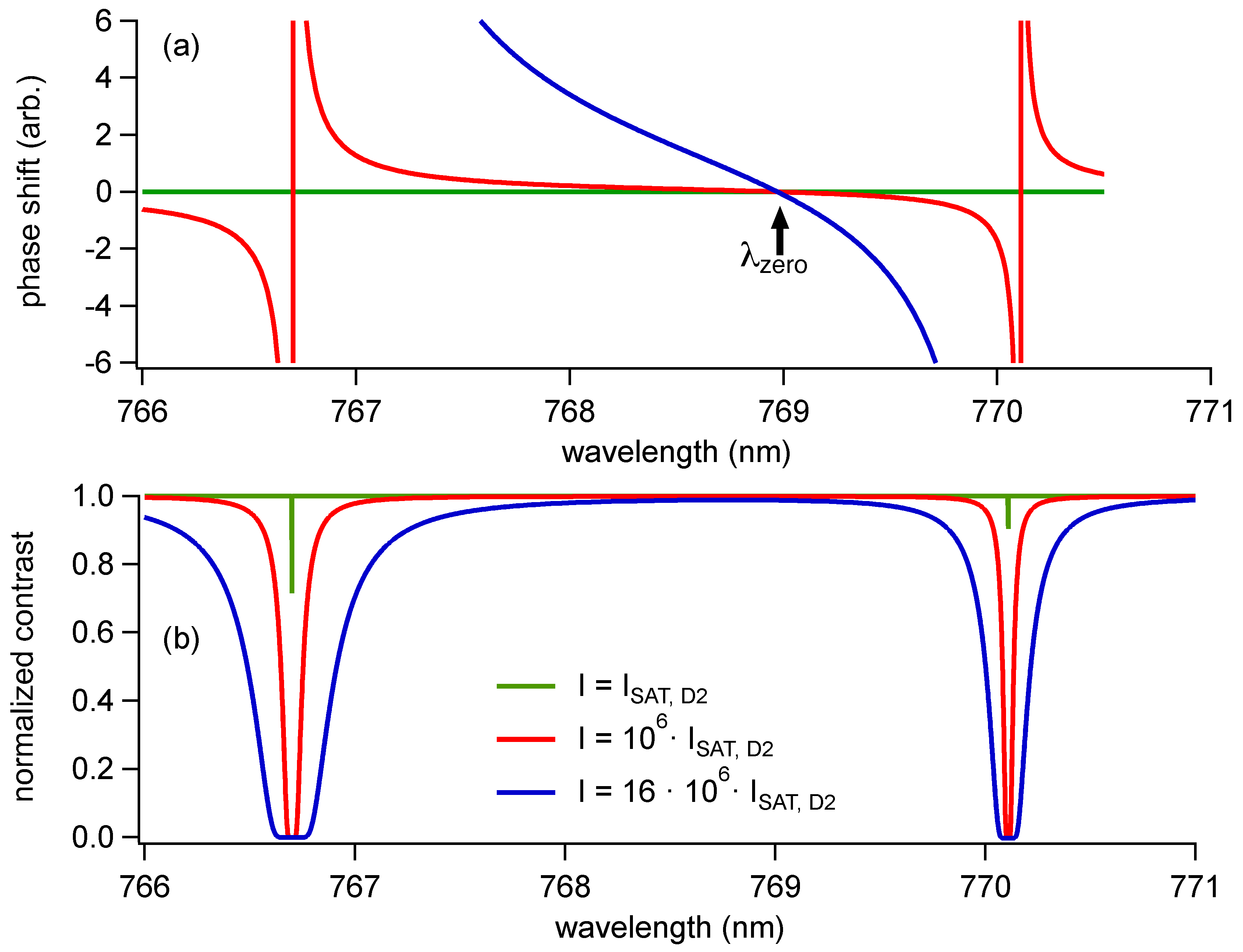
3. Decoherence Spectroscopy Model

To model the atom interferometer contrast, we start with the fact that scattering even one photon per atom reduces the atom interference fringe contrast nearly to zero if the components of each atom’s wave function are separated by a distance larger than the wavelength of light [3,6,7,8,9,10,11,13,18]. In one view, this is because each scattered photon conveys information about which path atoms traveled through the interferometer. In a related perspective, scattering entangles atoms with photons, and the photons constitute part of the atoms’ environment. Ignoring the state of the environment leads to observations of the atomic system with decreased coherence. Hence, atom interference fringe contrast that remains after interaction with the laser light is proportional to the probability $P_0\left(\omega \right)$ for atoms to scatter zero photons. We thus write the normalized contrast as

$$\frac{C_{\text{on}}}{C_{\text{off}}}=P_0\left(\omega \right).$$

(3)

The probability for an atom to scatter zero photons depends on the laser frequency ω, irradiance I, exposure time T, and the Doppler shift $\Delta \omega =\overrightarrow{v}·\overrightarrow{k}$, where $\overrightarrow{v}$ is atomic velocity and $\overrightarrow{k}$ is the laser beam propagation vector. We will start our model for $P_0\left(\omega \right)$ by considering a single laser beam.

The probability to scatter m photons is a Poisson distribution,

$$P_m=\frac{{\left(RT\right)}^m{e}^{-RT}}{m!},$$

(4)

where $R=R\left(\omega \right)$ is the photon scattering rate. Hence, the probability that an atom will not scatter any photons is $P_0\left(\omega \right)=e^{-RT}$. The scattering rate

$$R=\mathsf{\Gamma }{P}_{\text{ex}}\left(\omega \right)$$

(5)

depends on the natural decay rate Γ and the probability $P_{\text{ex}}\left(\omega \right)$ for atoms to be in the excited state. $P_{\text{ex}}\left(\omega \right)$ is the steady-state excited state population

$$P_{ex}\left(\omega \right)=\frac{{({\mathsf{\Omega }}_{\text{Rabi}}/2)}^2}{{(\omega -{\omega }_0)}^2+{(\mathsf{\Gamma }/2)}^2+{\mathsf{\Omega }}_{\text{Rabi}}^2/2}$$

(6)

where ${\mathsf{\Omega }}_{\text{Rabi}}$ is the Rabi frequency and ${\omega }_0$ is the resonance frequency for a two-level atom, as described in textbooks [40,41].

Next, we add an index F to account for the ground-state hyperfine splitting and an index p to account for different individual laser beams crossing the atom beam. Figure 3a,d show the probability for atoms in ground states $F=1$ and $F=2$ to be in the excited state, as a function of laser wavelength for a given laser beam $(p=0)$ with laser irradiance corresponding to ${\mathsf{\Omega }}_{\text{Rabi}}=6\mathsf{\Gamma }$ and ${\mathsf{\Omega }}_{\text{Rabi}}=24\mathsf{\Gamma }$, respectively. Figure 3 also shows the effect of power broadening. The probability of scattering zero photons from a particular laser beam (p) is then given by Equation (4) with $m=0$, combined with Equations (5) and (6):

$$P_{0,F,p}\left(\omega \right)=exp\left[\frac{-{({\mathsf{\Omega }}_{\text{Rabi}}/2)}^2\mathsf{\Gamma }T}{{(\omega -{\omega }_{0,F}-\Delta {\omega }_p)}^2+{(\mathsf{\Gamma }/2)}^2+{\mathsf{\Omega }}_{\text{Rabi}}^2/2}\right].$$

(7)

In a multi-pass optical cavity constructed with two plane mirrors, as shown in Figure 1, the Doppler shifts for each beam are different by the integer p times the angle θ between the two mirrors.

$$\Delta {\omega }_p=\left(p\theta +\delta \right)|\overrightarrow{v}\left|\right|\overrightarrow{k}|$$

(8)

where the parameter δ allows for asymmetry in the range of Doppler shifts (e.g., a residual or net Doppler shift that we will use our data to find). Here, the laser beam $p=0$ corresponds to the central beam, which is the last one before the laser beam propagation direction changes, and p ranges symmetrically from $-N$ to N. Figure 3b,e show the probability for atoms in ground states $F=1$ and $F=2$ to scatter zero photons from a single laser beam $(p=0)$ with power corresponding to ${\mathsf{\Omega }}_{\text{Rabi}}=6\mathsf{\Gamma }$ and ${\mathsf{\Omega }}_{\text{Rabi}}=24\mathsf{\Gamma }$, respectively.

The probability for an atom in one particular hyperfine level to scatter zero photons after interacting with the set of multiple laser beams in the MPC is given by the product

$$P_{0,F}\left(\omega \right)=\prod _{p=p_{min}}^{p_{max}}{P}_{0,F,p}\left(\omega \right).$$

(9)

To describe the contrast observed with an atom beam that is in a statistically random distribution of Zeeman $m_F$ states associated with the $F=1$ and 2 hyperfine levels, we average over all $m_F$ states to find

$$\frac{C_{\text{on}}}{C_{\text{off}}}=\sum _{F=1,2}\frac{{\gamma }_F}{A}{P}_{0,F}\left(\omega \right).$$

(10)

where ${\gamma }_F=2F+1$ is the degeneracy of each level, and the normalization constant $A={\sum }_F{\gamma }_F$. Condensing Equations (7)–(10), we obtain

$$\frac{C_{\text{on}}}{C_{\text{off}}}=\sum _F\frac{{\gamma }_F}{A}\prod _{p}exp\left[\frac{-{({\mathsf{\Omega }}_{\text{Rabi}}/2)}^2\mathsf{\Gamma }T}{{(\omega -{\omega }_{0,F}-\Delta {\omega }_p)}^2+{(\mathsf{\Gamma }/2)}^2+{\mathsf{\Omega }}_{\text{Rabi}}^2/2}\right].$$

(11)

Figure 3c,f show a model from Equation (11) for contrast, given an ensemble of atoms with initial populations randomly distributed in the hyperfine states associated with levels F = 1,2. The width and depth of the contrast-loss spectral features increases with more laser beams. The contrast only goes to zero at laser wavelengths for which atoms in both levels F = 1 and F = 2 scatter photons with high probability. This explains the shape of the contrast loss spectra. If the range of Doppler shifts (plus the power-broadened line widths) exceeds the hyperfine splitting, then the contrast goes to zero for a range of laser wavelengths. In our notation, the condition ${[{(\mathsf{\Gamma }/2)}^2+{\mathsf{\Omega }}_{\text{Rabi}}^2/2]}^{1/2}+\omega (p_{max}-p_{min})\theta (v/c)\ge ({\omega }_{0,2}-{\omega }_{0,1})$ is sufficient for contrast to be reduced to zero.

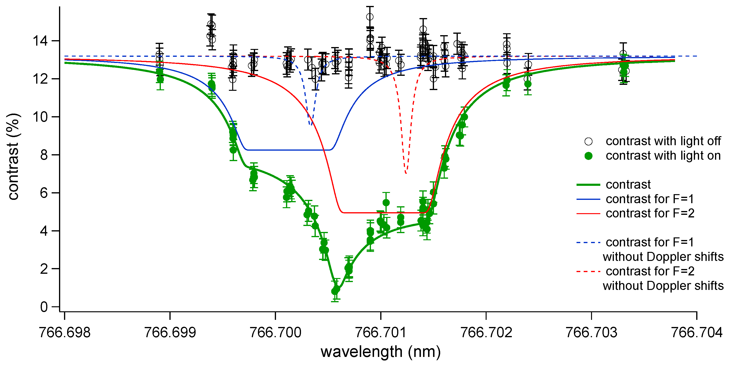
4. Decoherence Spectroscopy Data

Now we will compare the theoretical decoherence spectra derived with Equation (11) to data. To obtain decoherence spectroscopy data, we used the same laser and atom beam alignment as we did for phase shift, $\varphi \left(\omega \right)$, measurements. However, to obtain sharp spectral features, the laser wavelength is tuned near resonance, and the laser power is attenuated by several orders of magnitude so $\mathsf{\Omega }\approx \mathsf{\Gamma }$. We monitored the atom interference fringe contrast as a function of laser wavelength, as shown in Figure 4 and Figure 5. We measured the range $[p_{min},p_{max}]=[-38,38]$ and $\theta \approx 1.3$ mrad by counting the number of laser reflections and measuring the displacement of the reflected spots on the mirror. Our model for the decoherence spectrum given in Equation (10) then has free parameters ${\mathsf{\Omega }}_{\text{Rabi}}$, T, and δ.

Contrast data for different laser irradiance and associated models based on Equation (11) are shown in Figure 4. All parameters except ${\mathsf{\Omega }}_{\text{Rabi}}$—which is related to the laser beam irradiance—are the same for the models shown in Figure 4. We also note that δ was the same for all the data series shown in Figure 4, except for series shown in blue. The series in blue could be offset because of drifts in the alignment or the power of the laser beams during data acquisition. Slightly better fits for each individual data series shown in Figure 4 are possible if other parameters (such as T and θ) are allowed to be different for each series. This could be due to minor imperfections in the model that we discuss in Section 5.

A model decoherence spectrum, shown as a green line in Figure 5, makes the best fit to the decoherence spectra with $\delta =1.6^{\circ }\pm 0.4^{\circ }$, or a shift to the contrast spectrum of $-0.21\pm 0.05$ pm compared to a model with $\delta =0$. This uncertainty of 0.05 pm comes from a ${\chi }^2$ analysis of the data in Figure 5. We would like to interpret this observed shift as a correction that should be applied to a tune-out wavelength measurement due to the net Doppler shift in our experiment and also any systematic error of the Bristol 621B wavemeter that we used to measure the laser wavelength. However, we must slightly increase the uncertainty of this correction in order to allow for possible systematic errors in the difference between the Doppler shift for the contrast-loss spectra and the Doppler shift for the phase-shift spectra, as we discuss in the next section. Therefore, we apply a $+0.21\pm 0.10$ pm correction to our ${\lambda }_{\mathrm{zero}}$ measurement.

5. Discussion

Next, we will discuss complications with this experiment that are not yet accounted for in the the model we have presented. We also estimate the extent to which these complications can cause errors. Then, we will discuss some fundamental limits of decoherence spectroscopy and consider how well this method could be used to assess corrections to tune-out wavelength measurements in the future. We also compare this approach with other methods.

5.1. Complications and Suggested Improvements to Decoherence Spectroscopy Model

One complication is that the phase and contrast depend differently on the spatial profile of irradiance $I(x,y)$. The phase shift depends on irradiance gradients $\mathrm{d}/\mathrm{d}x[\int I(x,y)\mathrm{d}y]$, as shown in Equation (1), but decoherence only depends on the time of flight through the laser beam, which is related more simply to $\int I(x,y)\mathrm{d}y$. Hence, the variable size and position of the laser beam spots sketched in Figure 6 makes some laser beams contribute more to the phase shift signal, while different beams contribute more to the decoherence signal. This can be incorporated into more sophisticated models by making the Rabi frequency ${\mathsf{\Omega }}_{\text{Rabi},p}$, interaction time $T_p$, and the irradiance gradients $\mathrm{d}/\mathrm{d}x\left[I_p(x,y)\right]$ different for each beam number (p), as suggested by Figure 6.

To estimate the uncertainty caused by these factors, it is helpful to point out that the photon scattering probability can grow with the spot size w (for $I>I_{sat}$), but ϕ depends on $w^{-2}$. Hence, the tightly focused beams contribute much more to the phase shift signal. We estimate that the possible systematic error due to variable spot sizes could be as large as 0.08 pm in the present experiment, because the smallest spot is located—by design—very close to the symmetric point where the laser beam begins to turn around as it reflects back and forth and “walks” inside the MPC, as sketched in Figure 1 and Figure 6. We observed that the beam waist was within four spots of the turnaround point, and there were 19 beam spots on each mirror from the turnaround point to the first or last beams (entering or exiting) the MPC. From the spectra shown in Figure 4 and Figure 5, we determined that the extreme beams (with $p=+38$ or $p=-38$) are associated with a range of Doppler shifts that span 0.8 pm (i.e., $+0.4$ pm for the most red shifted and $-0.4$ pm for the most blue shifted beams, with respect to the beam at the turning point). Based on this information, we conclude that the phase-shift spectrum would have a net Doppler shift that is within 0.08 pm of the net Doppler shift for the decoherence spectra in Figure 5.

Our model of decoherence spectroscopy in Equation (11) could also be improved by including the effects of imperfect mirror reflectivity. This is another reason why the Rabi frequency ${\mathsf{\Omega }}_{\text{Rabi}}$ in Equations (10) and (11) should be replaced with a value ${\mathsf{\Omega }}_{\text{Rabi},p}$ that depends on the p index. We added this to our model and it changed the reported Doppler shift for contrast-loss spectra by less than 0.01 pm. This is a much smaller shift than the statistical uncertainty (0.05 pm) in the present experiment. We also note that the imperfect mirror reflectivity affects both the phase and the decoherence spectra in the same direction. So, the systematic error caused in ${\lambda }_{\mathrm{zero}}$ measurements from this imperfection in the model is negligible (smaller than 0.01 pm) in the present experiment.

Systematic differences between Doppler shifts for the phase and Doppler shift for the contrast spectra that are due to beam misalignment (as sketched in an extreme case in Figure 6b) are estimated to be smaller than 0.02 pm. To justify this estimate, we explain how the experiment was aligned. First, the mirrors making the MPC were adjusted with three piezo stacks so the string of laser spots entering and exiting the the MPC retrace their path, as sketched in Figure 6a. Then, the transverse position and overall rotation of the MPC assembly were adjusted in order to optimize (maximize) the phase shift. Furthermore, we note that the spots entering and exiting the MPC were much larger (greater than 0.5 mm in diameter), and these spots entered and exited approximately 1 cm from the turnaround point. With this geometry, it is nearly certain that all of the beams in the MPC contributed to the decoherence spectra. To estimate the uncertainty due to misalignment, we calculate that a 0.02 pm difference between phase and decoherence spectra Doppler shifts could occur if one of the large spots completely missed the atom beam.

In the model we have presented so far, we have not yet included the excited state hyperfine splitting. Instead, the model presented in Equations (7)–(11) and Figure 4 and Figure 5 represented a three level atom, with two ground levels ($4s_{1/2}$, F = 1, 2) and one excited level ($4p_{3/2}$). When we include hyperfine structure in the excited states, and use the Rabi frequency for each $\left|F,m_F\right.〉$ to $\left|F^{\prime },m_F^{\prime }\right.〉$ transition, the spectra change only slightly, and the resulting best fit shift is different by less than 0.001 pm. The fact that this shift is negligible was expected because the excited hyperfine splitting is not resolved in this experiment.

Contrast loss due to other mechanisms is an interesting topic in its own right. So, we discuss systematic errors due to dephasing in the next sub-section. We will conclude that dephasing also causes a small impact (<$0.01$ pm) on the best fit net Doppler shift of the contrast loss feature.

To summarize the error budget, we have considered errors and uncertainties due to complications to our model from variable laser beam spot sizes (<$0.08$ pm), imperfect mirror reflectivity (<$0.01$ pm), misalignment (<$0.02$ pm), and the excited state hyperfine splitting (<$0.001$ pm). Next, we will explain uncertainty (<$0.01$ pm) due to dephasing. Added in quadrature, all of these sources of uncertainty and the statistical uncertainty (0.05 pm) combine to make the total 0.10 pm uncertainty in the best fit shift for the decoherence spectroscopy feature.

5.2. Contrast Loss Mechanisms: Decoherence versus Dephasing

So far, the model for contrast loss that we have described in this paper only takes into account decoherence from photon scattering. However, there can also be contrast loss from dephasing—i.e., a distribution in light-induced phase for the ensemble of detected atoms. The origin of dephasing can be from the distribution in atomic velocity, from the distribution in the irradiance gradients across the thickness of the atom beam, or from the distribution of atomic spin states. We developed models of contrast loss from these dephasing mechanisms in order to study the relatively minor impacts on our decoherence spectra.

To understand why dephasing has less impact than decoherence near resonance, we point out that decoherence due to photon scattering in general depends on ${\Delta }^{-2}$, where Δ is the detuning from resonance. In comparison, the RMS spread in light-induced phase shifts generally depends on ${\Delta }^{-1}$. These differences are summarized in

Table 1. Dependence on I, Δ, and v for decoherence, dephasing, and phase shifts.

Observable in Presence of Laser	Dependence on I	Dependence on Δ	Dependence on v
C loss from decoherence	I	$1/{\Delta }^2$	$1/v$
C loss from dephasing	$|d^{2}I/d{x}^2|$	$|1/\Delta |$	${\sigma }_v/v$
light induced ϕ	$dI/dx$	$1/\Delta$	$1/v^2$

. Furthermore, contrast loss due to dephasing is mostly symmetric about line center, and therefore tends to slightly broaden but not shift the contrast loss feature.

Using calibration data far from resonance (with 500 pm detuning) and models of phase shifts, we found that dephasing due to the spread in velocity and the thickness of the atom beam (compounded with double gradients in irradiance) caused at most a 10% loss in contrast near line center. This is a small effect compared to decoherence. As mentioned earlier, this source of contrast loss is nearly completely symmetric about line center. The spectral offset from this dephasing is less than 0.001 pm. Dephasing due to the distribution of atomic spin states (taking into account both the ground and excited state hyperfine structure) was found to shift the best-fit contrast loss spectrum by less than 0.001 pm in models of our experiment for the conditions for the data in Figure 5. Based on these several models, we find that dephasing contributes an uncertainty of less than 0.01 pm to the spectral shift of the best-fit decoherence spectrum.

5.3. Comparison with Other Methods and Limits in Precision

Other methods of montoring the Doppler shift could be developed based on laser fluorescence spectroscopy, laser absorption spectroscopy, atom beam deflection spectra, or $\varphi \left(\omega \right)$. However, we argue that the decoherence spectroscopy method described here is as good—or better—than these other possible methods, because it only requires scattering one photon per atom and causes sharper spectral features. To compare methods in a bit more detail, since we have a flux of ${10}^7$ atoms per second passing through the multi-pass optical cavity, then if every atom scatters one photon, ${10}^7$ photons/s would be scattered. A geometric collection efficiency of ${10}^{-4}$ would be possible with the existing apparatus. This leaves a fluorescence signal of only 1000 photons per second, which would be challenging to distinguish from scattered light, given approximately 10 mW of light (${10}^{14}$ photons per second) incident on the multi-pass cavity. Similarly, it would be challenging to monitor the absorption of roughly 1 part in ${10}^7$. Atom beam deflection depends on laser frequency too, but decoherence is a more sensitive measure of deflection than any other tool we have. We emphasize that to make this experiment useful for ${\lambda }_{\mathrm{zero}}$ measurements, we use the same interaction region (optical beam geometry) for both the phase shift experiments and the decoherence experiments, and this sets some constraints on the optical access for hypothetical fluorescence and absorption measurements. Furthermore, using the same atom detector for both phase shift (${\lambda }_{\mathrm{zero}}$) and contrast-loss (decoherence) experiments helps to reduce any selection bias that would be caused by atoms that interact with laser light but fail to reach the atom detector. For all these reasons, decoherence spectroscopy is quite useful.

A fundamental limit for the precision of decoherence spectroscopy is related to the natural linewidth of atomic transitions, which is, for example, approximately 6 MHz, or 0.01 pm in the case of the potassium $4s-4p_{3/2}$ transition studied here. If the contrast spectrum features can be used to identify shifts as small as 1% of the natural linewidth (which is within the shot-noise limit for 15 min of data with a typical count rate of ${10}^5$ atoms/s), then Doppler shifts could be reported with an uncertainty of ${10}^{-4}$ pm or 0.05 MHz.

6. Conclusions

In this paper, we showed that matter wave decoherence due to photon scattering can be used to calibrate an atom interferometer spectroscopy experiment. We developed decoherence spectroscopy as a method to improve the accuracy of tune-out wavelength measurements made with an atom interferometer. Specifically, we demonstrated how decoherence is sensitive to the net Doppler shift for an atom beam passing through a multi-pass optical cavity and possible systematic errors in wavemeter calibration. We presented a theoretical model of decoherence spectra and experimental contrast-loss data with curious spectral features that qualitatively validate the model. This model and these data informed us that $0.21\pm 0.10$ pm should be added as a correction to the tune-out wavelength (${\lambda }_{\mathrm{zero}}$) measurements made with this apparatus. Furthermore, this correction depends somewhat sensitively on the alignment and location of the laser beam waist within the interaction region.

References

1. Zurek, W.H. Environment-induced superselection rules. Phys. Rev. D 1982, 26, 1862–1880. [Google Scholar] [CrossRef]
2. Zurek, W.H. Decoherence and the transition from quantum to classical. Phys. Today 1991, 44, 36–44. [Google Scholar] [CrossRef]
3. Zurek, W.H. Decoherence, einselection, and the quantum origins of the classical. Rev. Mod. Phys. 2003, 75, 715–775. [Google Scholar] [CrossRef]
4. Joos, E.; Zeh, H.D. The emergence of classical properties through interaction with the environment. Z. Phys. B Condens. Matter 1985, 59, 223–243. [Google Scholar] [CrossRef]
5. Caldeira, A.O.; Leggett, A.J. Influence of damping on quantum interference: An exactly soluble model. Phys. Rev. A 1985, 31, 1059–1066. [Google Scholar] [CrossRef]
6. Joos, E.; Zeh, H.D.; Kiefer, C.; Giulini, D.J.; Kupsch, J.; Stamatescu, I.O. Decoherence and the Appearance of a Classical World in Quantum Theory; Springer Science & Business Media: Berlin, Germany, 2013. [Google Scholar]
7. Chapman, M.S.; Hammond, T.D.; Lenef, A.; Schmiedmayer, J.; Rubenstein, R.A.; Smith, E.; Pritchard, D.E. Photon scattering from atoms in an atom interferometer: Coherence lost and regained. Phys. Rev. Lett. 1995, 75, 3783–3787. [Google Scholar] [CrossRef] [PubMed]
8. Kokorowski, D.A.; Cronin, A.D.; Roberts, T.D.; Pritchard, D.E. From single- to multiple-photon decoherence in an atom interferometer. Phys. Rev. Lett. 2001, 86, 2191–2195. [Google Scholar] [CrossRef] [PubMed]
9. Uys, H.; Perreault, J.D.; Cronin, A.D. Matter-wave decoherence due to a gas environment in an atom interferometer. Phys. Rev. Lett. 2005, 95, 150403. [Google Scholar] [CrossRef] [PubMed]
10. Hornberger, K.; Uttenthaler, S.; Brezger, B.; Hackermüller, L.; Arndt, M.; Zeilinger, A. Collisional decoherence observed in matter wave interferometry. Phys. Rev. Lett. 2003, 90, 160401. [Google Scholar] [CrossRef] [PubMed]
11. Hackermüller, L.; Hornberger, K.; Brezger, B.; Zeilinger, A.; Arndt, M. Decoherence of matter waves by thermal emission of radiation. Nature 2004, 427, 711–714. [Google Scholar] [CrossRef] [PubMed]
12. Myatt, C.J.; King, B.E.; Turchette, Q.A.; Sackett, C.A.; Kielpinski, D.; Itano, W.M.; Monroe, C.; Wineland, D.J. Decoherence of quantum superpositions through coupling to engineered reservoirs. Nature 2000, 403, 269–273. [Google Scholar] [PubMed]
13. Haroche, S. Entanglement, decoherence and the quantum/classical boundary. Phys. Today 1998, 51, 36–42. [Google Scholar] [CrossRef]
14. Martinis, J.M.; Nam, S.; Aumentado, J.; Lang, K.M.; Urbina, C. Decoherence of a superconducting qubit due to bias noise. Phys. Rev. B 2003, 67, 094510. [Google Scholar] [CrossRef]
15. Wang, H.; Hofheinz, M.; Ansmann, M.; Bialczak, R.C.; Lucero, E.; Neeley, M.; O’Connell, A.D.; Sank, D.; Weides, M.; Wenner, J.; et al. Decoherence dynamics of complex photon states in a superconducting Circuit. Phys. Rev. Lett. 2009, 103, 200404. [Google Scholar] [CrossRef] [PubMed]
16. Roszak, K.; Filip, R.; Novotný, T. Decoherence control by quantum decoherence itself. Sci. Rep. 2015, 5, 9796. [Google Scholar] [CrossRef] [PubMed]
17. Roszak, K.; Machnikowski, P. A which path decoherence in quantum dot experiments. Phys. Lett. A 2006, 351, 251–256. [Google Scholar] [CrossRef]
18. Clauser, J.F.; Li, S. “Heisenberg microscope” decoherence atom interferometry. Phys. Rev. A 1994, 50, 2430–2433. [Google Scholar] [CrossRef] [PubMed]
19. Kunze, S.; Dieckmann, K.; Rempe, G. Diffraction of atoms from a measurement induced grating. Phys. Rev. Lett. 1997, 78, 2038–2041. [Google Scholar] [CrossRef]
20. Gupta, S.; Dieckmann, K.; Hadzibabic, Z.; Pritchard, D. Contrast interferometry using Bose-Einstein condensates to measure h/m and α. Phys. Rev. Lett. 2002, 89, 140401. [Google Scholar] [CrossRef] [PubMed]
21. Eibenberger, S.; Cheng, X.; Cotter, J.P.; Arndt, M. Absolute absorption cross sections from photon recoil in a matter-wave interferometer. Phys. Rev. Lett. 2014, 112, 250402. [Google Scholar] [CrossRef] [PubMed]
22. LeBlanc, L.J.; Thywissen, J.H. Species-specific optical lattices. Phys. Rev. A 2007, 75, 053612. [Google Scholar] [CrossRef]
23. Safronova, M.; Williams, C.J.; Clark, C.W. Relativistic many-body calculations of electric-dipole matrix elements, lifetimes, and polarizabilities in rubidium. Phys. Rev. A 2004, 69, 022509. [Google Scholar] [CrossRef]
24. Arora, B.; Safronova, M.S.; Clark, C.W. Tune-out wavelengths of alkali-metal atoms and their applications. Phys. Rev. A 2011, 84, 043401. [Google Scholar] [CrossRef]
25. Topcu, T.; Derevianko, A. Tune-out wavelengths and landscape-modulated polarizabilities of alkali-metal Rydberg atoms in infrared optical lattices. Phys. Rev. A 2013, 88, 053406. [Google Scholar] [CrossRef]
26. Mitroy, J.; Tang, L.Y. Tune-out wavelengths for metastable helium. Phys. Rev. A 2013, 88, 052515. [Google Scholar] [CrossRef]
27. Le Kien, F.; Schneeweiss, P.; Rauschenbeutel, A. Dynamical polarizability of atoms in arbitrary light fields: General theory and application to cesium. Eur. Phys. J. D 2013, 67, 1–16. [Google Scholar] [CrossRef]
28. Jiang, J.; Mitroy, J. Hyperfine effects on potassium tune-out wavelengths and polarizabilities. Phys. Rev. A 2013, 88, 032505. [Google Scholar] [CrossRef]
29. Jiang, J.; Tang, L.Y.; Mitroy, J. Tune-out wavelengths for potassium. Phys. Rev. A 2013, 87, 032518. [Google Scholar] [CrossRef]
30. Cheng, Y.; Jiang, J.; Mitroy, J. Tune-out wavelengths for the alkaline-earth-metal atoms. Phys. Rev. A 2013, 88, 022511. [Google Scholar] [CrossRef]
31. Safronova, M.S.; Zuhrianda, Z.; Safronova, U.I.; Clark, C.W. The magic road to precision. ArXiv e-prints 2015. [Google Scholar]
32. Yu, W.W.; Yu, R.M.; Cheng, Y.J. Tune-out wavelengths for the Rb atom. Chin. Phys. Lett. 2015, 32, 123102. [Google Scholar] [CrossRef]
33. Chamakhi, R.; Ahlers, H.; Telmini, M.; Schubert, C.; Rasel, E.; Gaaloul, N. Species-selective lattice launch for precision atom interferometry. New J. Phys. 2015, 17, 123002. [Google Scholar] [CrossRef]
34. Herold, C.D.; Vaidya, V.D.; Li, X.; Rolston, S.L.; Porto, J.V.; Safronova, M.S. Precision measurement of transition matrix elements via light shift cancellation. Phys. Rev. Lett. 2012, 109, 243003. [Google Scholar] [CrossRef] [PubMed]
35. Holmgren, W.F.; Trubko, R.; Hromada, I.; Cronin, A.D. Measurement of a wavelength of light for which the energy shift for an atom vanishes. Phys. Rev. Lett. 2012, 109, 243004. [Google Scholar] [CrossRef] [PubMed]
36. Leonard, R.H.; Fallon, A.J.; Sackett, C.A.; Safronova, M.S. High-precision measurements of the 87RbD-line tune-out wavelength. Phys. Rev. A 2015, 92, 052501. [Google Scholar] [CrossRef]
37. Keith, D.W.; Ekstrom, C.R.; Turchette, Q.A.; Pritchard, D.E. An interferometer for atoms. Phys. Rev. Lett. 1991, 66, 2693–2696. [Google Scholar] [CrossRef] [PubMed]
38. Berman, P. Atom Interferometry; Academic Press: San Diego, CA, USA, 1997. [Google Scholar]
39. Cronin, A.D.; Schmiedmayer, J.; Pritchard, D.E. Optics and interferometry with atoms and molecules. Rev. Mod. Phys. 2009, 81, 1051–1129. [Google Scholar] [CrossRef]
40. Metcalf, H.J.; van Straten, P. Laser Cooling and Trapping; Springer: New York, NY, USA, 1999. [Google Scholar]
41. Foot, C.J. Atomic Physics; OUP Oxford: Oxford, UK, 2004. [Google Scholar]
Figure 1. (a) Top-view schematic of a three-grating Mach–Zehnder atom interferometer passing through an optical cavity; (b) Side-view schematic of the plane–plane optical cavity aligned so atoms interact with multiple passes of the laser beam. Both atom beam paths shown in (a) are represented by one thick line and pass through the cavity in (b). The atom beam paths are each 30 μ m thick and have a 10 μ m separation between them. The mirror angle deviation from parallel ( θ ) is exaggerated to show how the laser beam folds back at different angles.
Atoms 04 00025 g001
Figure 2. Phase shift and contrast loss spectra for potassium atoms, simulated for different amounts of laser power using Equations (1), (2) and (11). λ zero is the root in the phase shift spectrum in between two resonances. Contrast loss due to photon scattering occurs near the D1 and D2 resonances. We use the sharpest features of (b) to calibrate λ zero measurements modeled in (a).
Atoms 04 00025 g002
Figure 3. Decoherence spectroscopy model. Graphs (a,d) show the probability of finding atoms in an excited 4 p state of K 39 while exposed to laser light with wavelength λ = 2 π c / ω and irradiance such that Ω Rabi = 6 Γ (a) or 24 Γ (d). Graphs (b,e) show the probability of scattering zero photons ( P 0 , F ) after atoms pass through a laser beam, as described by Equation (7) with an interaction time of T = 3 / Γ , and Ω Rabi = 6 Γ or 24 Γ , respectively. Graphs (c,f) show Contrast after passing through multiple laser beams as described by Equation (9) with parameters θ = 1.3 mrad, δ = 0. The red and blue curves show the contrast for the atoms in a specific F level with a single laser beam ( p = 0 ), and the solid black curve shows the combined contrast for the ensemble of atoms. The thinner black curves show the contrast for varying number of laser beams interacting with the atom beam, using ( N p N , with N = 1, 3, 9, 18, 35, or 50).
Atoms 04 00025 g003
Figure 4. Decoherence spectra showing contrast as a function of wavelength. Theoretical curves based on Equation (11) with T = 3 / Γ and θ = 1 . 3 mrad are shown too. The laser power (hence the parameter Ω Rabi ) was deliberately varied for the different data sets. Higher irradiance results in deeper and broader contrast loss features. The red, orange, green, and black fits show a net Doppler shift of −0.21 pm. The fit in blue shows a net Doppler shift of −0.48 pm, but we suspect the laser power may have drifted during this data set, thus causing a spurious shift in the line center.
Atoms 04 00025 g004
Figure 5. Contrast data spectrum (green points) and model (green line). The dashed red and blue lines show contrast spectra for each hyperfine ground state with no Doppler shift. The model has parameters Ω Rabi = 6 . 2 Γ , T = 3 / Γ , θ = 1 . 3 mrad, and δ = 28 . 3 mrad, which corresponds to a net Doppler shift of 0 . 21 ± 0 . 05 pm.
Atoms 04 00025 g005
Figure 6. Top view of the multi-pass cavity with a schematic representation of the atom beams (purple) and the laser spots (red). Different alignments can result in different Doppler shifts and irradiance gradients for the laser beams that illuminate the atom beam. (a) The mirror angles are adjusted so the laser spots propagating in y ^ overlap with those propagating in + y ^ . This configuration is used for tune-out wavelength measurements; (b) The mirror angles are adjusted such that the laser spots propagating in y ^ and + y ^ do not overlap.
Atoms 04 00025 g006