Estimating Relative Uncertainty of Radiative Transition Rates

Atomic Spectroscopy Group, Quantum Measurements Laboratory, National Institute of Standards and Technology (ret.); Gaithersburg, MD 20899-8422, USA
Atoms 2014, 2(4), 382-390; https://doi.org/10.3390/atoms2040382
Submission received: 31 January 2014
/
Revised: 16 September 2014
/
Accepted: 9 October 2014
/
Published: 25 November 2014
(This article belongs to the Special Issue Critical Assessment of Theoretical Calculations of Atomic Structure and Transition Probabilities)
Abstract
:We consider a method to estimate relative uncertainties of radiative transition rates in an atomic spectrum. Few of these many transitions have had their rates determined by more than two reference-quality sources. One could estimate uncertainties for each transition, but analyses with only one degree of freedom are generally fraught with difficulties. We pursue a way to empirically combine the limited uncertainty information in each of the many transitions. We “pool” a dimensionless measure of relative dispersion, the “Coefficient of Variation of the mean,” . Here, for each transition rate, “s” is the standard deviation, and “” is the mean of “n” independent data sources. is bounded by zero and one whenever the determined quantity is intrinsically positive.) We scatter-plot the as a function of the “line strength” (here a more useful radiative transition rate than transition probability). We find a curve through comparable s that envelops a specified percentage of the s (e.g. 95%). We take this curve to represent the expanded relative uncertainty of the mean. The method is most advantageous when the number of determined transition rates is large while the number of independent determinations per transition is small. The transition rate data of Na III serves as an example.
Our goal is to optimize uncertainty estimates for published radiative transition rates by “pooling” relative uncertainties of these rates within a spectrum. Most evaluated transition rates have been accurately determined by two or fewer sources (experimental and/or theoretical). In such cases it is generally difficult to make useful distribution-based estimates of uncertainty for individual transitions. Fortunately, there are many transitions in any given atomic spectrum. Here we propose a graphical method for empirically estimating relative uncertainties by “pooling” relative standard deviations of transition rates within a spectrum.
As we shall see, this “heterogeneous” pooling can result not only in improved uncertainty estimates of transition rates, but also in detecting outliers and interpolating transition rate uncertainties that have only one reference-quality determination. First we must find an appropriate measure of relative dispersion.
Consider a given transition with an ensemble {xi} of “n” independent determinations of radiative line strength. Each ensemble has a mean “” and unbiased standard deviation “s”. The Coefficient of Variation, , is defined as:
For our purposes, it will be more useful to consider a slightly modified quantity.
Consider a large-n population {xi}. Say we take different samples “j” from this population. The central limit theorem holds that the mean of such samples {} will have a standard deviation of approximately , the standard deviation of the mean. Here, is the jth sample mean and . Therefore, as a matter of nomenclature, we refer to:
as the Coefficient of Variation of the mean. The properties of are discussed in Kelleher [1]. This article presents the required proofs and considers in detail the advantages and limitations of heterogeneous pooling.
For a population {xi} of size n, has the useful limit (with condition):
That is, the coefficient of variation of the mean is intrinsically bounded by zero and one if all determined quantities (such as line strengths (S)) are positive. This normalization property of is useful. One knows automatically the quantitative significance of with regard to one. Also, in Equation (3), the upper limit is independent of n. This makes it feasible to pool multiple sources with a different n value.
For each transition rate, when n = 2:
Note that the upper bound on Equation (4a) is 1 whenever x> is positive.
In general, for each transition rate j having nj independent determinations, and mean , the Coefficient of Variation of the mean is:
As for a specific transition rate, we choose to pool the variation of the line strength (S), rather than transition probabilities or oscillator strengths. This is necessary because S is proportional to the radial matrix element only. Thus, transition energies and statistical weights do not enter (the former can be quite large). This allows us to pool transitions with different transition energies and statistical weights. (The term “transition rate” is used loosely here to refer collectively to the three radiative entities, S, A, and f. Each of the three can be converted to either of the others by using expressions in [2], for example.)
Below we describe the three steps of this empirical pooling method. We begin by scatter-plotting the of different transitions of the same spectrum as a function of the logarithm of the mean line strength. Next, we fit a least-squares curve through the data to determine the “slope” of the data. Finally, using this slope, we iteratively derive a second curve which envelops the specified fraction p of data points. We take this envelope curve to represent the expanded relative uncertainty of the mean, . (The term “expanded” refers to the specified value of p (e.g. 95%); the “+” denotes the upper bound. To the extent possible, we use the terminology of the International Organization for Standardization [3]). This “GUM” does not consider the coefficient of variation. We use Tp+ to indicate the upper confidence bound of the Coefficient of Variation, and to designate the expanded relative uncertainty of the mean. Such plots can also illuminate systematic trends and outliers.
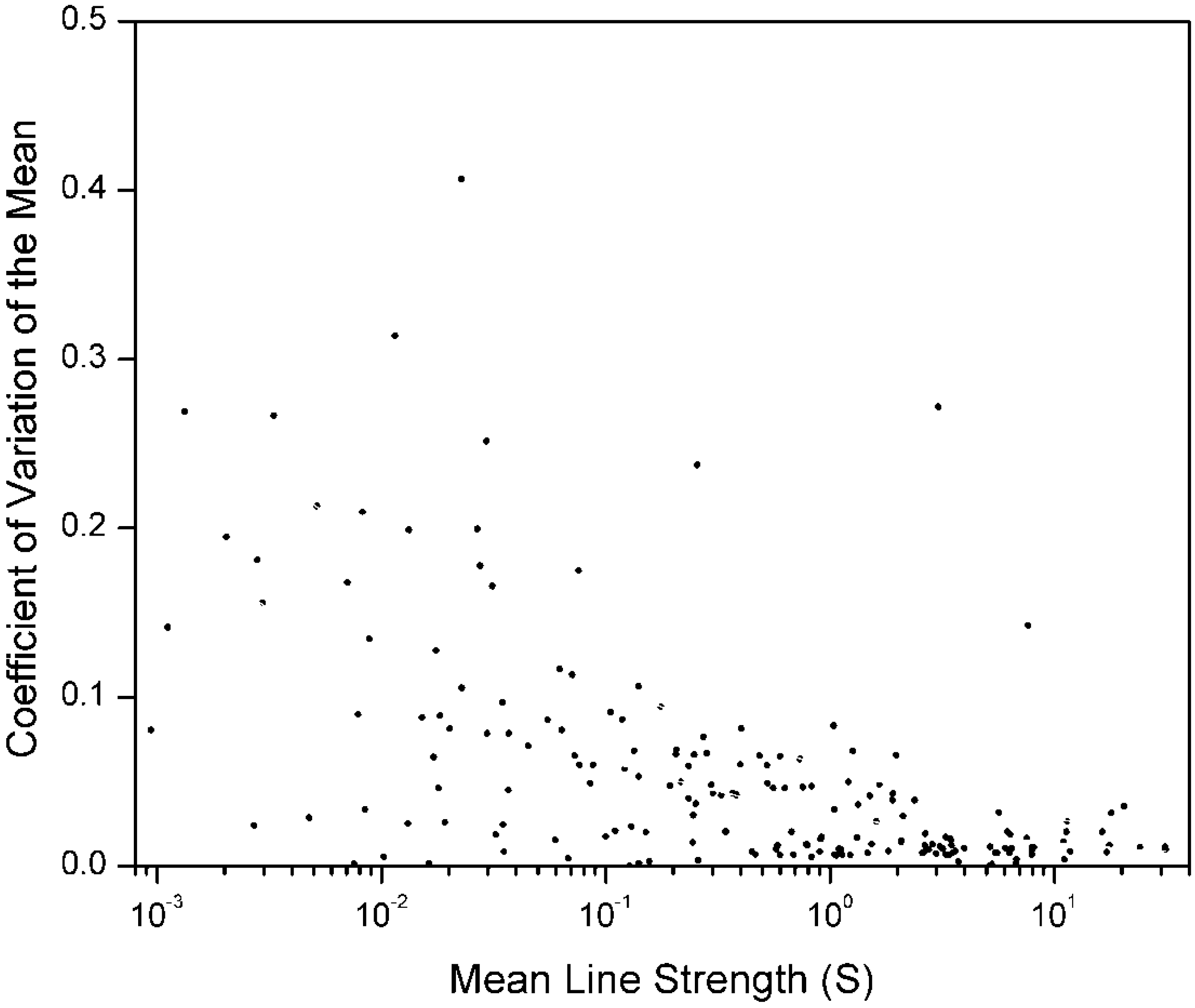
In Figure 1, we plot the for 192 radiative transition rates of the spectral lines of doubly ionized sodium (Na III). These rates were calculated by two different theoretical approaches: the “Multi-configuration Hartree–Fock” method, (Tachiev and Froese Fischer [4]), and the “Configuration Interaction” method (McPeake and Hibbert [5]). The for each transition in this figure, given by Equation (4a), contains only one degree of freedom (n = 2, ν = 1). Only transitions from energy levels above 415,000 cm−1 are included in this figure.
The two parameters of the lower fit curve are determined initially by least square fitting. Except in special cases, there is no a priori relationship between and the sample mean. However, for satisfying Equation (3), any fitting functions Φ0 must have asymptotic bounds of one and zero. We have chosen:
See Figure A1 in Appendix A. Here erfc is the complimentary error function, erfc = 1 – erf. An algorithm for computing erf is given in the appendix. and β are fit parameters analogous to “intercept” and “slope”, respectively. Φ0() has asymptotic values of one and zero, consistent with Equation (3). This ad hoc fit curve has the equivalent functional form to the cumulative distribution function of the log-normal distribution.
After the scatter-plot, the second step in our heterogeneous pooling procedure involves the determination of parameters β[LS], and . We perform a Levenberg–Marquardt nonlinear LS fit for Equation (6) using the implementation in the “C” language by Press et al. [6]. This enables us to evaluate the two parameters for the LS curve (lower). (An equation like Equation (6) exists for each “Coefficient of Variation of the mean,” and Line Strength Sj. In Equation (6), the “” symbol is meant to indicate a LS “best-fit” for the two LS fit parameters).
Finally, keeping this same fit value of β[LS], we estimate an expanded relative uncertainty of the mean, , by iterating [p] in Equation (7) to determine a second, higher curve such that a specified fraction p of the s fall beneath it. (Using a different β for the LS and curves would lead to the physically impossible consequence that the two curves would cross at some point).
Figure 1.
The mean line strength vs. the Coefficient of Variation of the mean, , for radiative transition rates in Na III for which the energy of the upper level is greater than 415, 000 cm−1. Seven outliers, three of which are off the scale, were given very small weights. Because only two data sources are used, the for each transition is given by Equation (4a).
This empirical method for “covering” any specified percentage of does not require random data or the existence of any particular pdf. It does depend on the validity of heterogeneously pooling the of different line strengths within the spectrum. We take the curve to be an empirical analog to the upper confidence bound of the mean for the normally-distributed Coefficient of Variation of the mean, , with the distinction that incorporates, to some level of approximation, the effects of both random and systematic errors. (A website by Verrill [7] calculates for Normal and log-Normal distributions). LS fit curves can generally be determined more precisely than, for example, 95% envelope curves, because the latter are heavily influenced by the small percentage of points lying outside them. If relative uncertainties for any “outliers” are assigned, this should be done independently of the heterogeneous pooling considered here.
This heterogeneous pooling method has proven effective for critical evaluations of transition rates in recent NIST compilations of more than 90 different atomic and ionic spectra, for which we use p = 0.90. (See, for example, Kelleher and Podobedova [2].) We apply a correspondence table between the value on the envelope curve, , and the letter-grade given in the compilation. We also interpolate this envelope curve when only one datum source is available (n = 1) for a given transition. (The number of degrees of freedom vanishes for , but not for the curve .)
Thus far we have described a method for estimating the envelope curve that represents the expanded relative uncertainty of the mean as a function of the mean line strength, . The key assumption in the heterogeneous pooling of the coefficient of variation of the mean (relative standard deviations of the mean), is that pooled s are comparable. Below we consider ways to discern whether any members are not appropriate contributors to . They may belong to a separate subgroup or they may be outliers. The latter usually appear as isolated points on a curve.
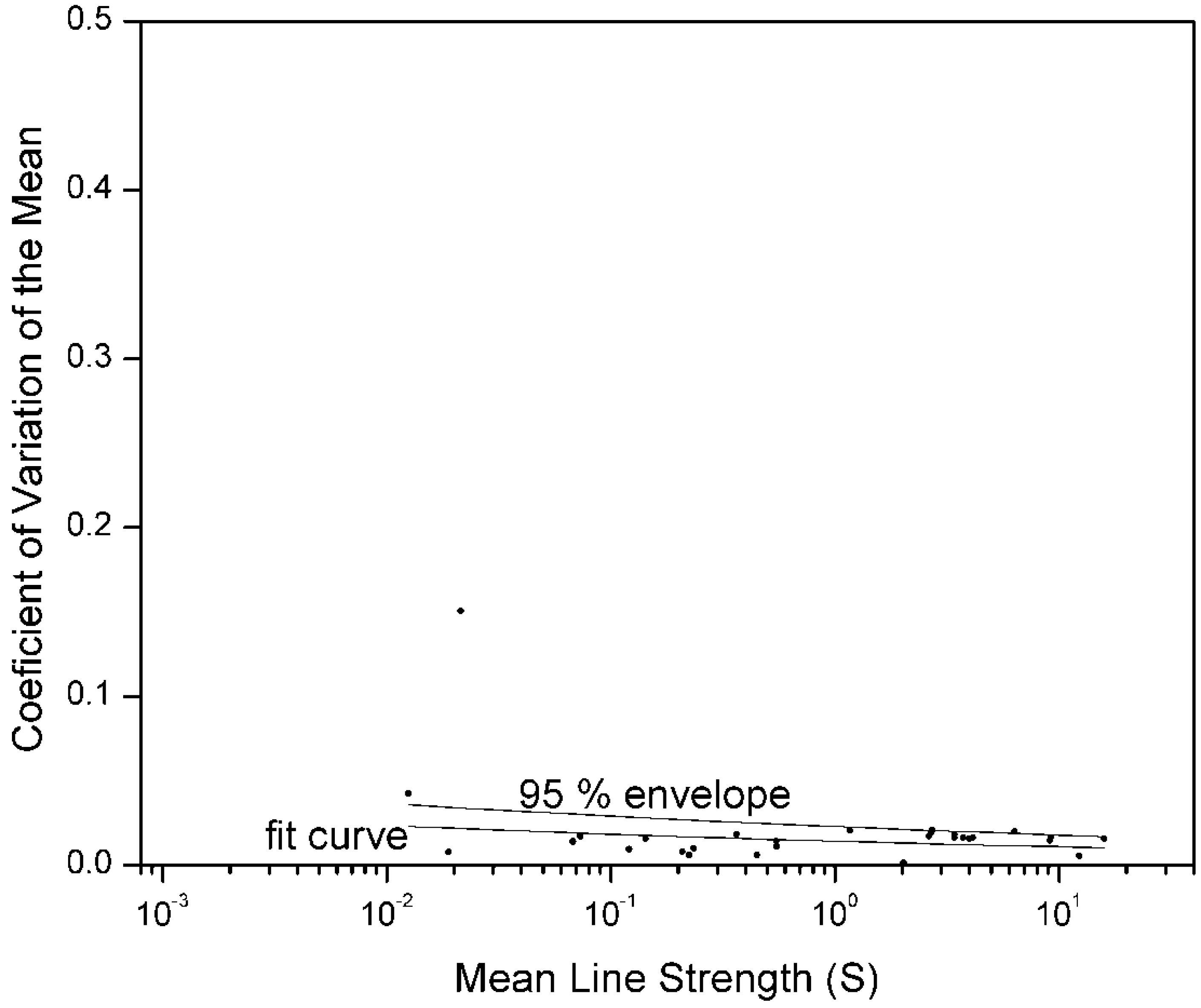
Comparison of Figure 2 with Figure 3 illustrates the importance of pooling comparable s. The data in Figure 3 are limited to transitions from lower-lying levels, for which the energy of the upper level is less than 415,000 cm−1. These levels belong to the same Na III spectrum, but are more widely spaced than the upper levels of the Figure 2 transitions. Thus level “mixing” is less for transitions from lower-lying levels. This results in smaller computational discrepancies between the two methods. If we had not separated out the data for Figure 3, we would have overestimated the relative uncertainty for this data.
Figure 2.
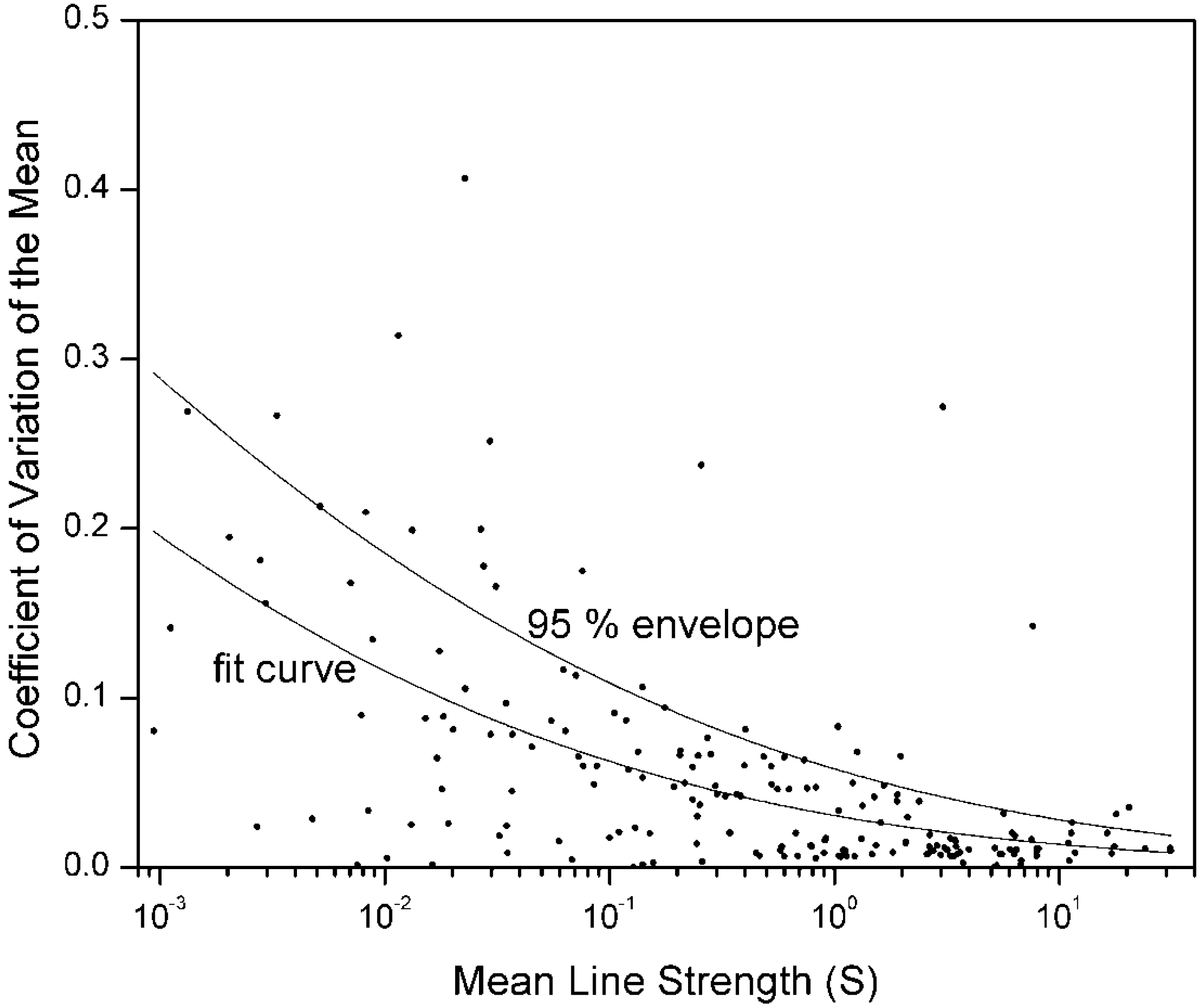
The data points are the same as Figure 1, to which two curves have been added. Seven outliers, three of which are off the scale, were given small weights. Because only two data sources were used, the for each transition is given by Equation (4a). For the lower curve, parameters β[LS] and [LS] in Equation (6) were evaluated by a LS fit, and β[LS] was found to be 4.2 (“slope”). Keeping the same β, [p] was then adjusted in Equation (7) until 95% of the points (excluding outliers) lie under the upper curve, for which [p] = 5.1 × 10⁻⁵ (“intercept”). Compare to Figure 3.
Figure 2.
The data points are the same as Figure 1, to which two curves have been added. Seven outliers, three of which are off the scale, were given small weights. Because only two data sources were used, the for each transition is given by Equation (4a). For the lower curve, parameters β[LS] and [LS] in Equation (6) were evaluated by a LS fit, and β[LS] was found to be 4.2 (“slope”). Keeping the same β, [p] was then adjusted in Equation (7) until 95% of the points (excluding outliers) lie under the upper curve, for which [p] = 5.1 × 10⁻⁵ (“intercept”). Compare to Figure 3.

Figure 3.
Coefficient of Variation of the mean () for radiative transitions in Na III in which the energy of the upper level is less than 415,000 cm−1, in contrast to Figure 1 and Figure 2. One value was weighted as an outlier. Each point is the for a different radiative transition. These data were taken from the same sources as in Figure 2, and the scales are the same. Ninety-five percent of the points lie beneath the upper curve, for which β = 13.8 and = 2.3 × 10⁻¹⁹.
Subsets of can sometimes lie significantly below the envelope curve, . It may be that some of these are best treated separately from heterogeneous pooling, if justified by expert knowledge or self-consistency of within the subset. We can test for subgroups of s by computing for each transition rate the ratio of its to the envelope curve (), and sorting the ratio.
In the curve fitting, all values are given a weight of one except those which lie more than a factor of three above or below the envelope curve. Such “outliers” are given a weight inversely proportional to the square of their distance from this envelope curve, and thus have negligible influence on the fit. Distant outliers can destabilize a LS solution.
s that lie above the pooled envelope (but do not qualify as outliers) can also be identified by inspection of the plot, such as in Figure 2 and Figure 3. For the fraction 1-p of values that lie above the envelope curve, we approximate their relative uncertainties by equating them to their individual s.
In summary, we describe a pooling method to estimate expanded relative uncertainties of the mean for atomic transition rates. We consider cases where a small number of independent determinations have been made for a substantial number of transition rates from the same spectrum. Let where, for each transition, s is the standard deviation and is the mean of n independent determinations of the transition rate. Scatter-plotting s from these sources vs. , typically enables one to heterogeneously pool them. By finding a curve which covers a specified fraction “p” (e.g. 95%) of the , one estimates the expanded relative uncertainty of the mean, , as a function of . It includes random and systematic errors. The envelope curve can also facilitate the detection of outliers and interpolation of relative uncertainties for which only one transition strength has been determined. Estimating relative uncertainties for theoretical transition rates of Na III serves as an example of the method.
Acknowledgments
The author gratefully acknowledges vital contributions by Mark Vangel and William Guthrie.
Appendix A:
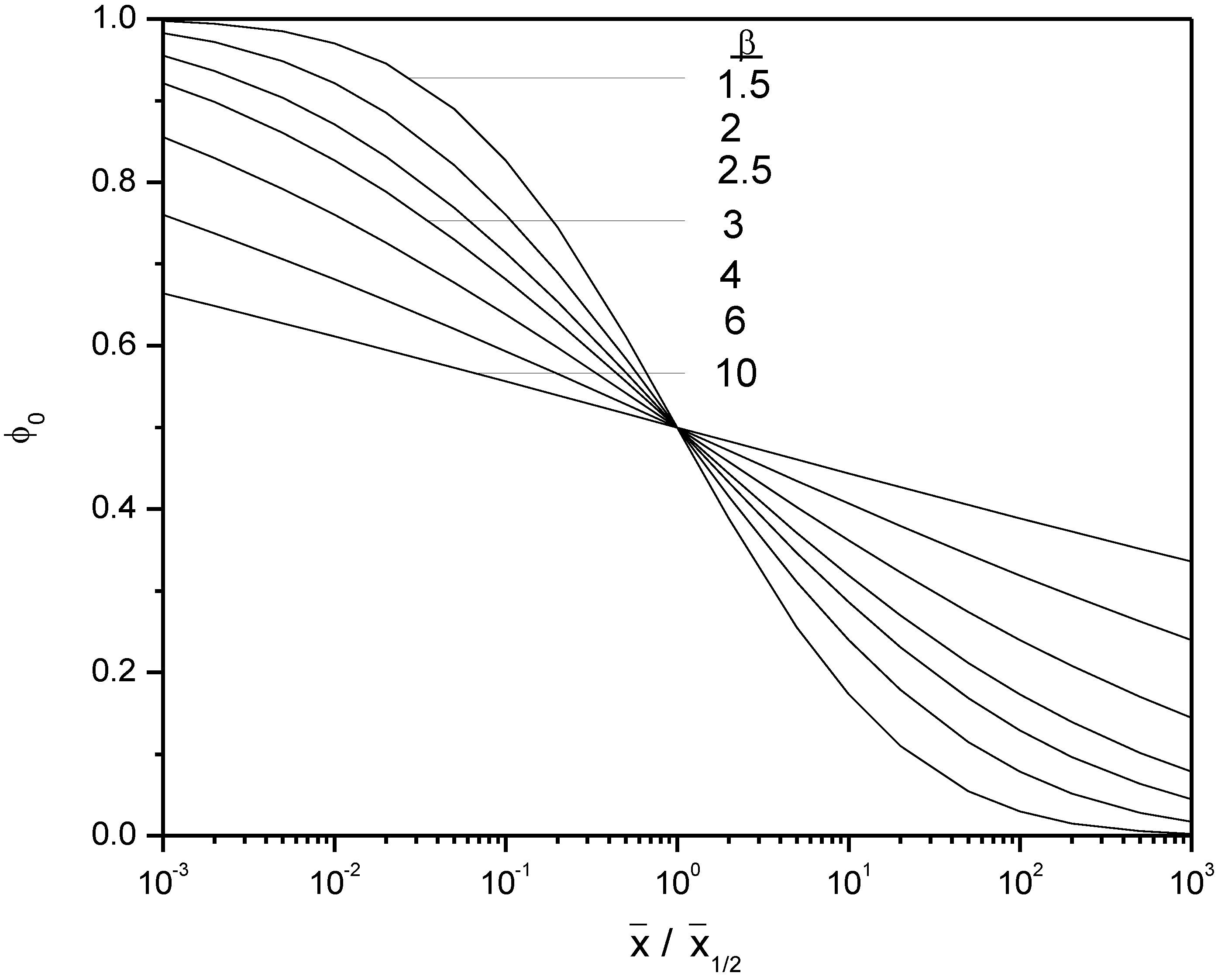
Figure A1 displays Equation (5) as a function of for seven values of β ranging from 1.5 to 10. The only required properties of Equation (5) are that it has the appropriate asymptotes and has a weak monotonic dependence on . Except for poor data, smaller Φ0() prevail (i.e., <≈ 0.3). Φ0 has proven robust in fitting a wide range of different data types, including those that span essentially the entire range of 0 to 1. Other functional forms may work better for different data sets. The whole procedure could also be performed graphically, without the explicit use of a parametric fitting function.
Figure A1.
The fitting function Φ0(), Equation (5), for the Coefficient of Variation of the mean as a function of for seven values of β. The mean is represented by and is the value of the mean for which = 0.5.
Figure A1.
The fitting function Φ0(), Equation (5), for the Coefficient of Variation of the mean as a function of for seven values of β. The mean is represented by and is the value of the mean for which = 0.5.
Anomalous cases can arise, for example, when the does not approach zero at asymptotically large values of . In some cases we add a term that is constant as approaches zero and vanishes as Φ0() approaches one, such as:
We recommend using Equation (8) only when the data clearly indicate an asymptote greater than zero. This can happen when one data set (usually inferior) lies consistently above the others. It is unlikely to be a good candidate for pooling. One should always plot the individual candidates for pooling, to check against systematic differences.
Appendix B:
Error Function:
The error function is defined as:
An efficient numerical recipe, accurate to 1.5 × 10⁻⁷, is given by Hastings [8] (slightly modified here):
where:
and
also, if z < 0, erf(z) = −erf(z).
erf(z) = 1 – p exp(−z2),
p = f·(0.254829592 + f·(−0.284496736 + f·(1.421413742 + f·(−1.453152027 + f·1.061405429)))),
Conflicts of Interest
The authors declare no conflict of interest.
References
- Kelleher, D.E.; (National Institute of Standards and Technology, Gaithersburg, USA). Empirical Estimates of Relative Uncertainty. Unpublished work. 2014. [Google Scholar]
- Kelleher, D.E.; Podobedova, L.I. Atomic transition probabilities of sodium and Magnesium. A critical complication. J. Phys. Chem. Ref. Data 2008, 37, 267–706. [Google Scholar] [CrossRef]
- International Organization for Standardization. Guide to the Expression of Uncertainty in Measurement (GUM); International Organization for Standardization: Geneva, Switzerland, 1995; Section 6, Annex G. [Google Scholar]
- Tachiev, G.; Froese Fischer, C. Breit Pauli energy levels, lifetimes, and transition data: Na II and Na III. Available online: http://nlte.nist.gov/MCHF/view.html (accessed on 30 December 2002).
- McPeake, D.; Hibbert, A. Transitions in Na III. J. Phys. B 2000, 33, 2809–2832. [Google Scholar] [CrossRef]
- Press, W.H.; Teukolsky, S.A.; Vetterling, W.T.; Flannery, B.P. Numerical Recipes in C; Cambridge University Press: Cambridge, UK, 1992. [Google Scholar]
- Verrill, S. Exact confidence bounds for a normal distribution coefficient of variation. Available online: http://www1.fpl.fs.fed.us/covnorm.dcd.html (accessed on 30 December 2002).
- Hastings, C. Approximations for Digital Computers; Princeton University Press: Princeton, NJ, USA, 1955. [Google Scholar]
© 2014 by the authors; licensee MDPI, Basel, Switzerland. This article is an open access article distributed under the terms and conditions of the Creative Commons Attribution license (http://creativecommons.org/licenses/by/4.0/).
Share and Cite
MDPI and ACS Style
Kelleher, D.E. Estimating Relative Uncertainty of Radiative Transition Rates. Atoms 2014, 2, 382-390. https://doi.org/10.3390/atoms2040382
AMA Style
Kelleher DE. Estimating Relative Uncertainty of Radiative Transition Rates. Atoms. 2014; 2(4):382-390. https://doi.org/10.3390/atoms2040382
Chicago/Turabian StyleKelleher, Daniel E. 2014. "Estimating Relative Uncertainty of Radiative Transition Rates" Atoms 2, no. 4: 382-390. https://doi.org/10.3390/atoms2040382