Circular Geodesics, Paczyński-Witta Potential and QNMs in the Eikonal Limit for Ayón-Beato-García Black Hole


Department of Physics, Hiralal Mazumdar Memorial College For Women, Dakshineswar, Kolkata-700035, India
Universe 2018, 4(3), 55; https://doi.org/10.3390/universe4030055
Submission received: 1 December 2017
/
Revised: 24 February 2018
/
Accepted: 27 February 2018
/
Published: 13 March 2018
(This article belongs to the Special Issue Black Hole Thermodynamics)
Abstract
:We investigate the comprehensive geodesic structure of a spherically symmetric, static charged regular Ayón-Beato and García black hole (BH). We derive the equation of innermost stable circular orbit (ISCO), marginally bound circular orbit (MBCO) and circular photon orbit (CPO) of said BH, which are most relevant to BH accretion disk theory. Using time-like geodesic properties, we derive Paczyński-Witta potential form for this BH which are very relevant to determine the general relativistic effects on the accretion disk. We show that at a certain radius (For example in case of Reissner-Nordstrøm (RN) BH, ), there exists zero angular momentum (ZAM) orbits due to the repulsive gravity. We also show that in the eikonal approximation, the real and imaginary parts of the quasi normal modes (QNM) of the regular BHs can be expressed as in terms of the frequency of the BH and the instability time scale of the unstable null circular geodesics. Moreover, we study the Bañados, Silk and West effect for this BH. We show that the center-of-mass (CM) energy of colliding neutral test particles near the infinite red-shift surface of the regular BHs have the finite energy. In the Appendix section, we have discussed the possibility of a regular ABG BH can act as particle accelerators when two charged test particles of different energies are colliding and approaching to the horizon of the BH provided that one of charged test particle has a critical value of charge.
1. Introduction
Geodesic motion of test particles (both timelike and lightlike) for various BHs spacetime namely Schwarzschild BH, RN BH, Kerr BH, Kerr-Newman BH have been studied by various authors in different way [1,2,3,4,5,6,7]. This is the only method of experimental verification of gravitaional fields of compact object like BHs. They are the most fascinating compact objects in the universe. They predicted different types of observable effects in the general relativity that can be tested in our solar system. For example, the gravitational redshift, the gravitational bending of light, gravitational time-delay or Shapiro time-delay, Perihelion precession of light, gravitational lensing and Lense-Thirring effect, etc. all are the physical effects which are directly connected to the study of geodesic structure of the BH. Therefore, it is very crucial to study the geodesic properties of the BH spacetime.
In order to understand the geodesic motion for masive particles of a given spacetime it is necessary to know the timelike geodesic equation which can be written as
where is Christoffel symbols.
Similarly for massless particles, the geodesic equation is given by
where is affine parameter.
Among different kind of geodesics, circular geodesics, particularly ISCOs, are more interesting. Circular geodesic motion in the equatorial plane is of fundamental interest in BH physics as well as in accretion disk physics to determine the important features of the spacetime. Circular orbits with are stable, while those with are not. Keplerian circular orbits exist in the region , with being the circular photon orbit. Bound circular orbits exist in the region , with being the marginally bound circular orbit, and stable circular orbits exist for , with . We have calculated these orbits for the above regular BHs. These orbits are very crucial in BH physics as well as in astrophysics because they determine important information on the back ground geometry.
The conventional BHs like Schwarzschild BH, RN BH, Kerr BH and Kerr-Newman BHs have possessed a curvature singularity. Whereas the regular BH [8,9,10,11,12,13,14,15] does not have any curvature singularity. This is the main differences between the conventional BH and the regular BH. On the other hand, it is also important to understand the final state of gravitational collapse of initially regular configurations of the BH, that’s why we need to study the global regularity of BH solutions. Broadly speaking for conventional BHs, the curvature invariants blows up at in the spacetime manifold, while for regular BHs the curvature invariants do not blow up everywhere in the spacetime manifold including at . In this sense, it is said to be a “regular BH” or “non-singular BH”.
We have considered here regular Ayón-Beato and García (ABG) BH [9]. The special features of these BHs are they have satisfied the weak energy condition (WEC) and the energy-momentum tensor should have the symmetry . Our goal here is to study the BSW effect for these BHs.
There are a number of references we would like to mention here which discuss some interesting properties of the regular BHs. Firstly, Ansoldi [16] gave a good review of the regular BH. Balart [17] studied the Brown-York quasi-local energy and Komar energy at the horizon which is called Bose-Dadhich identity [18], and proved that this identity does not satisfied for the regular BHs. In [19], the author showed that Smarr’s formula do not satisfied in case of the regular Bardeen and ABG space-time. In [20], the authors have been studied the weak energy condition of the regular BH. Recently, García et al. [21] have discussed the complete geodesic structure of ABG spacetime by using Weierstrass elliptic functions. Finally, Eiroa et al. [22] have discussed the gravitational lensing effect of the regular Bardeen BH (See also [23]). The QNM of test fields around different regular BHs have been studied in [24].
However, in this work, we have studied the complete geodesic structure of neutral test particle motion of a regular Ayón-Beato and García BH. We have derived the ISCO, MBCO and CPO of the said BHs, which are most important to BH accretion disk physics. We have also derived Paczyński-Witta [25] potential for ABG BH which is so called pseudo-Newtonian potential. Paczyński-Witta potential could be used to describe the general relativistic effects on the accretion disk properties. Not only that this potential could help us to determine the approximate solutions of the hydrodynamical equations. The interesting feature of Paczyński-Witta potential is that it could help us to determine the right positions of the ISCO and MBCO of the BH. For Schwarzschild BH, Paczyński-Witta was first determined such features and for Kerr BH, this potential has derived by Mukhopadhyay [26]. In this work, we have applied this method for ABG BH.
In addition to that we have computed the QNM frequency for the said regular BHs in the eikonal limit. It has been shown that this frequency of the BH can be expressed in terms of the parameters of the unstable null circular geodesics. Moreover, we have examined the Bañados, Silk and West (hereafter BSW) [27] effect for this kind of BHs.
Geodesic properties have been considered previously for the said BH first in the Ref. [21] by using Weierstrass elliptic functions method. After that the geodesic properties considered for regular Bardeen BH, ABG BH and Hayward BH extensively by using Chandrasekhar’s approach in [4]. Subsequently in [28], the authors considered the geodesic properties for ABG BH and Bardeen BH by using the features of no-horizon structure of the BHs. From the author’s best of knowledge, previously pseudo-Newtonian potential & QNM frequency for regular ABG BH in the eikonal limit have not been considered in the literature.
The paper is organized as follows. In Section 2, we would describe the geodesic motion of neutral test particles in the back ground of ABG space-time. In Section 3, we would study the QNMs of null circular geodesics in the eikonal limit. In Section 4, we would study the BSW effect for regular ABG BH and finally we summarize the results in Section 5. In the appendix section, we should examine the possibility of a regular BH could be act as particle accelarators when two charged particles are colliding near the vicinity of the horizon of the BH.
2. Equatorial Circular Orbits in ABG Space-Time
In this section, we will investigate the geodesic motion of neutral test particles for a ABG BH. This space-time is also a regular BH space-time and singularity free solutions of the coupled system of a non-linear electrodynamics and general relativity. The source is a nonlinear electrodynamic field satisfying the WEC, which in the limit of weak field becomes the Maxwell field. We find the CM energy for this space-time can be infinitely high when the BH is only extremal. Before computing the CM energy we shall demonstrate shortly the geodesic structure of the ABG space-time.
The metric of the ABG space-time [9,13,14,15,21,29] is given by
where the function is defined by
where m is the mass of the BH and q is the monopole charge. The strength of the radial electric field is given by
We can see the behaviour of the function graphically in Figure 1.
This is also a first regular BH solution in general relativity. The source is a nonlinear electrodynamic field satisfying the WEC, which in the limit of weak field becomes the Maxwell field.
It may also be noted that this metric function asymptotically behaves as the RN space-time [9] i.e.,
The ABG BH has an event horizon which occurs at . i.e.,
The variation of radial horizon function for different values of q could be seen in Figure 2. In the limit , we shall get the horizon of the Schwarzschild BH i.e., . The ABG space-time represents a regular BH when . The value of is . When , there are two horizons in the ABG space-time, we call it non-extremal ABG space-time as in the non-extremal RN space-time.
When , the two horizons are coincident at , which corresponds to an extreme ABG BH as in the RN BH. The Carter-Penrose diagram of ABG space-time is quite similar structure to the RN BH.
To derive the complete geodesic structure of the Bardeen BH we shall follow the pioneering book by S. Chandrasekhar [1] and J. B. Hartle [2]. To compute the geodesic motion of the test particle in the equatorial plane we set and . Since the space-time admits two Killing vectors namely, and . Therefore the quantities and are conserved along the geodesics, is the four velocity of the particle. Where E and L can be interpreted as conserved energy and conserved angular momentum per unit mass respectively.
Thus, in this coordinate chart, E can be written as
and, L can be expressed as in terms of the metric
From the normalization condition of the four velocity for massive particles we find
where for time-like geodesics, for light-like geodesics and for space-like geodesics.
The radial equation that governs the geodesic structure in the ABG space-time reads [4]
where the effective potential for the geodesic motion of the ABG space-time is given by
2.1. Particle Orbits
(i) The Effective Potential
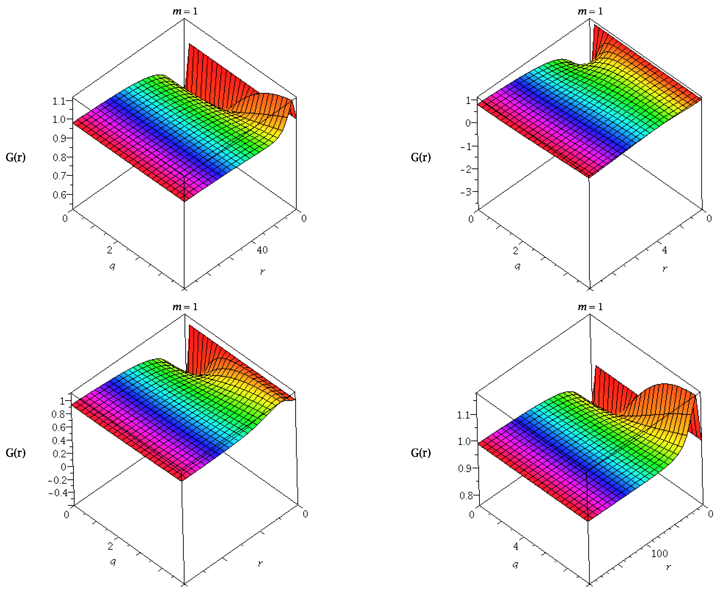
The effective potential for time-like geodesics can be written as using the Equation (11) by setting
Analogously, for zero angular momentum geodesics the effective potential becomes
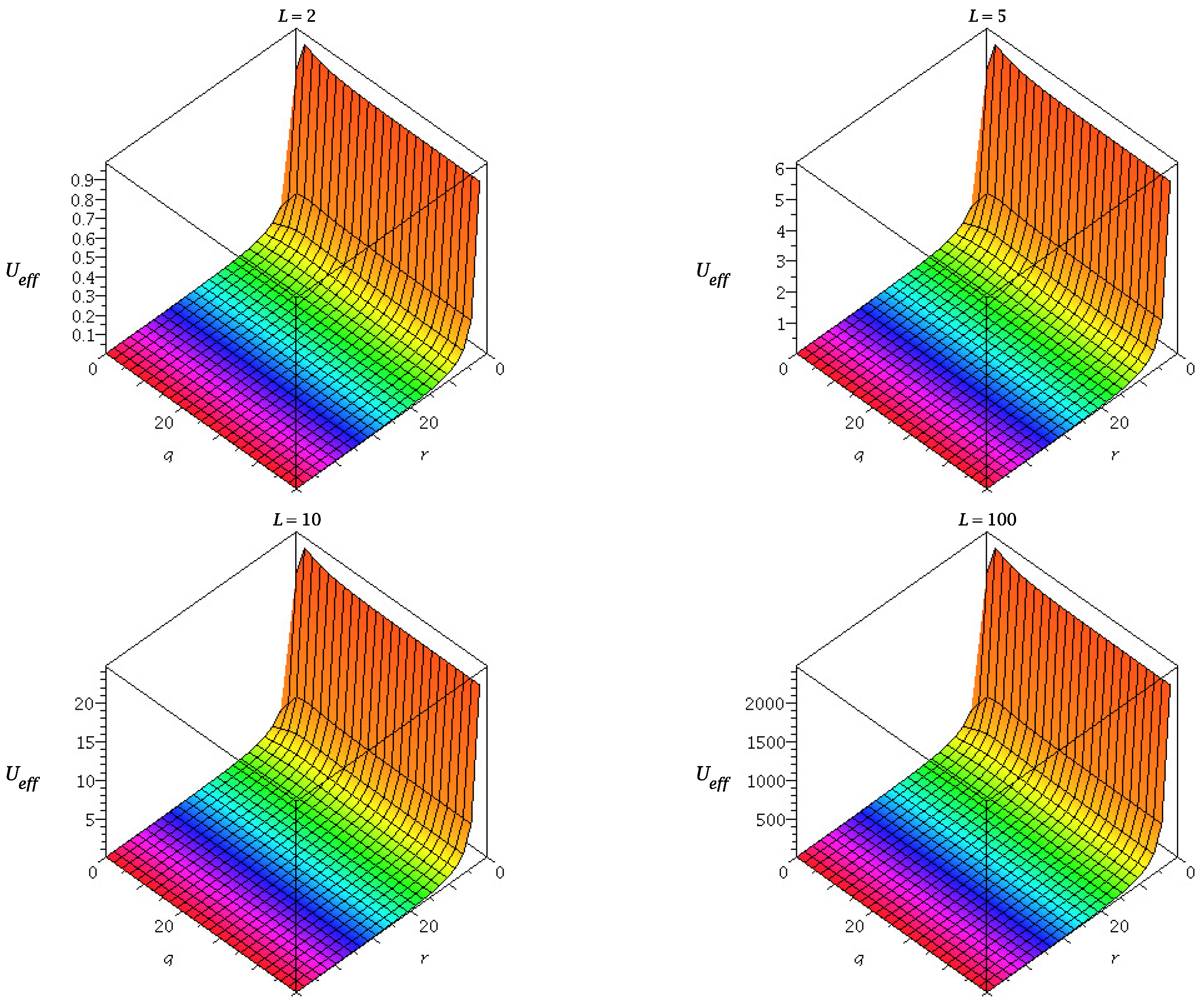
The trajectories of the test particle in the zero angular momentum potential well can be seen from the Figure 3.
Similarly, the geodesic motion of neutral test particles can be studied by using the effective potential diagram which is plotted in Figure 4.
Similarly, to derive the circular geodesic motion of the test particle in ABG space-time, we must use the condition at . From Equation (11), one gets
and
Thus one can obtain the energy and angular momentum per unit mass of the test particle along the circular orbits [4]
and,
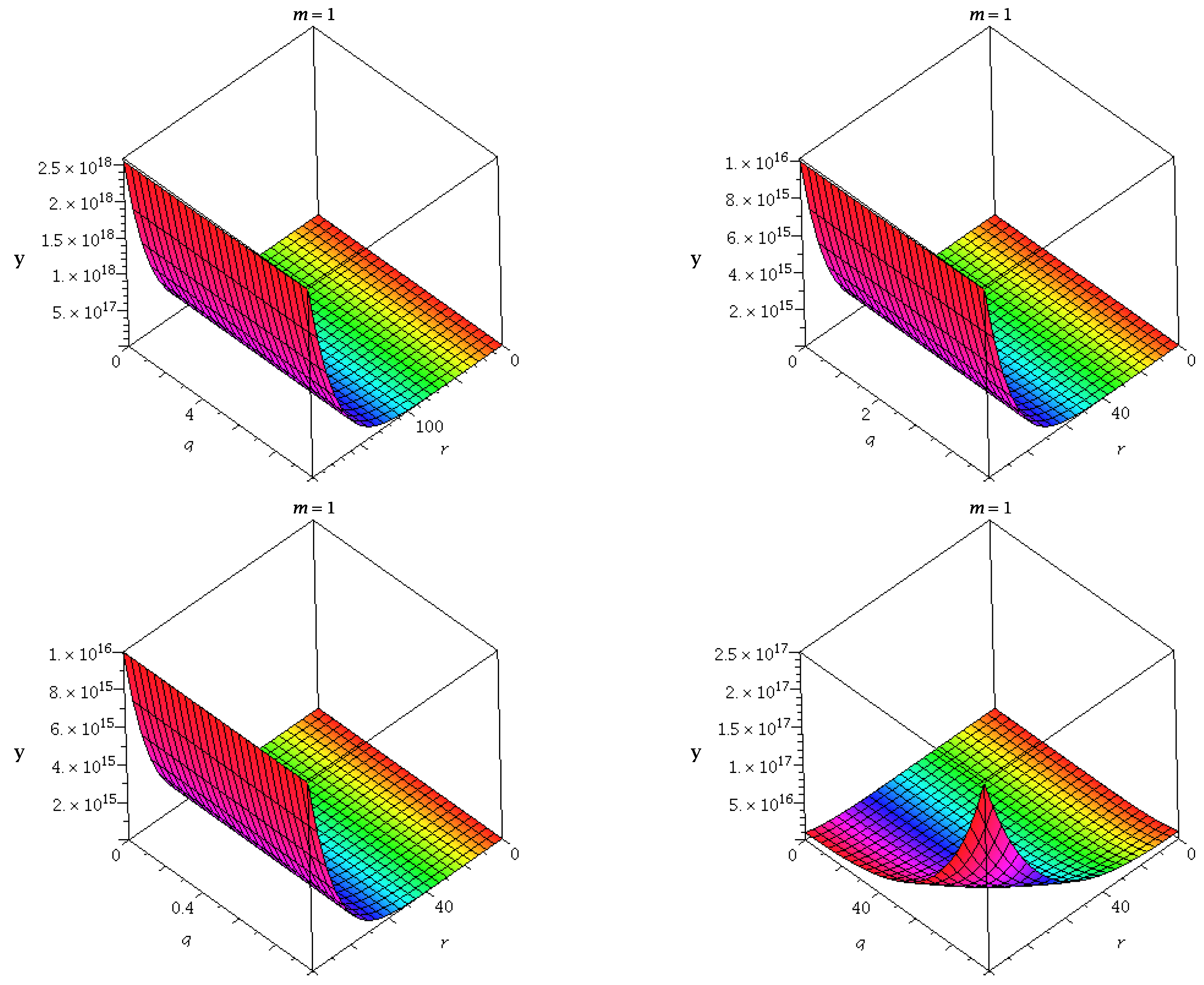
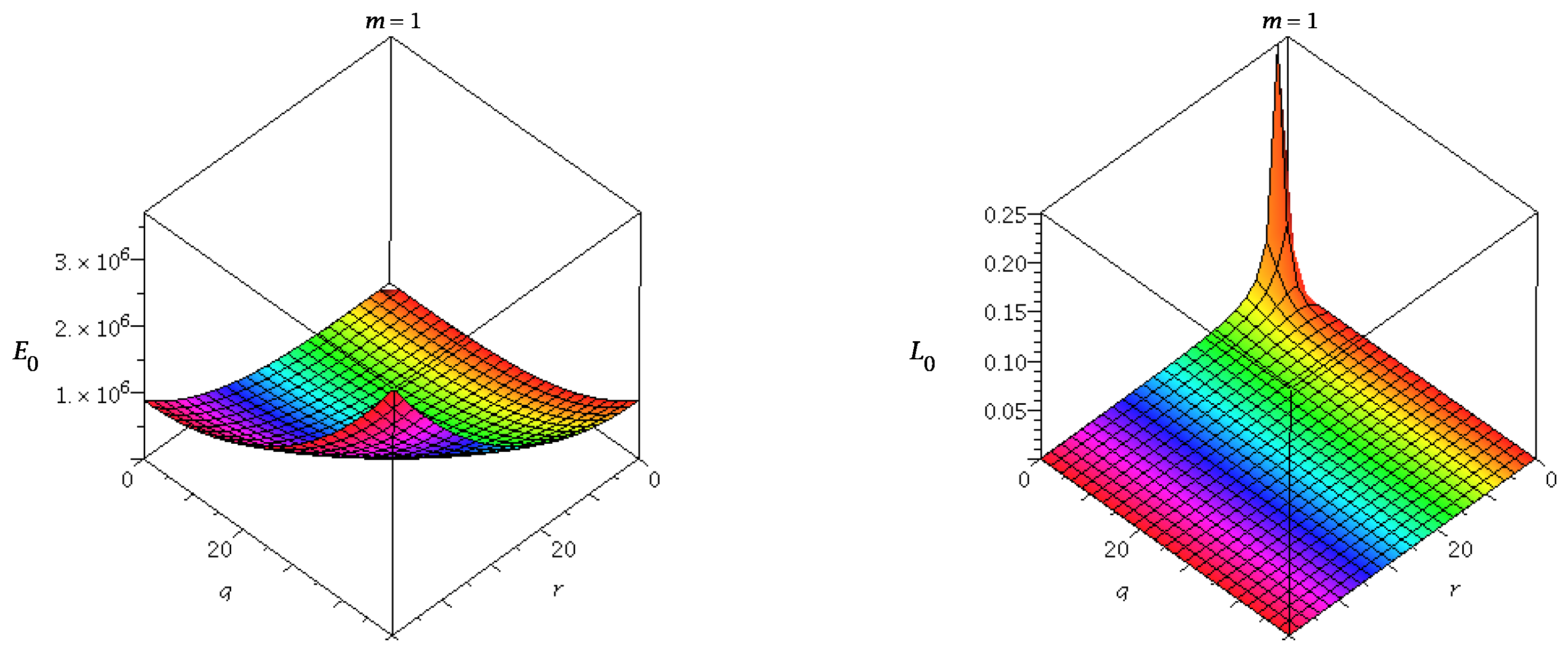
Circular motion of the test particle to be exists for ABG space-time when both energy and angular momentum are real and finite. The 3D diagram of variation of energy and angular momentum along circular orbits could be seen from Figure 5.
Thus we get the inequality
and
Circular orbits do not exist for all values of r, so from Equations (17) and (18), we can see that the denominator would be real only when
or
The limiting case of equality indicates a circular orbit with diverging energy per unit rest mass i.e., a photon orbit. This photon orbit is the inner most boundary of the circular orbits for time-like particles.
It could be expected that the ZAM orbit exists due to the repulsive gravity at the radius where for ABG BH as we have seen in case of Bardeen spacetime. Due to the mathematical difficulty we could not determine the exact radius but we could say that it is a polynomial equation of sixth order. Whereas this orbit exists for RN BH at the static radius [5,30] which has been mentioned earlier in the abstract.
The equation of MBCO [4] for ABG space-time looks like
Let be the solution of the equation which gives the radius of MBCO close to the BH.
The ISCO equation could be obtain from the second derivative of the effective potential of time-like case i.e.,
Let be the real solution of Equation (23) which gives the radius of the ISCO of ABG space-time. In the limit , we obtain the radius of ISCO for Schwarzschild BH which occurs at .
(ii) The Paczyński-Witta Potential
Here we should derive the pseudo-Newtonian potential for ABG following the Ref. [26]. This pseudo-Newtonian potential is often called Paczyński-Witta (PW) Potential for Schwarzschild BH because PW first derived this potential for Schwarzschild BH. This potential is useful tool for studying BH astrophysics. Although the charge is not considered in realistic astrophysical situations we have derived this potential for ABG BH purely from theoretical point of view. This is the motivation behind to derive this potential. It should be noted that this potential has been derived in the equatorial plane. The interesting features of this potential is that it could be used to determine the locations of the ISCO and MBCO of BH. To derive it first we should calculate the Keplerian angular distribution following the Ref. [26]
Now we introduce the variables and then one could write the corresponding centrifugal force for ABG BH
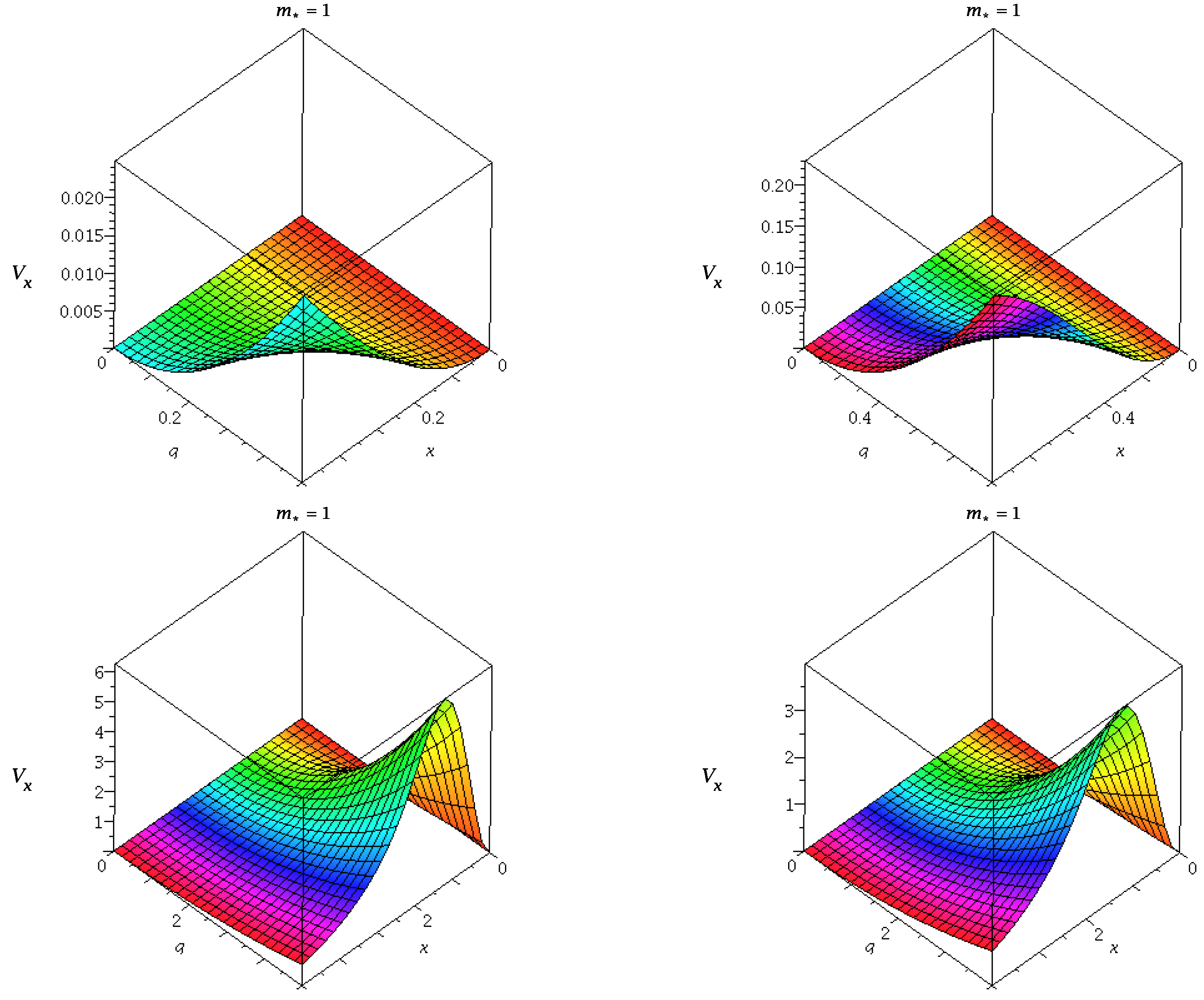
The above equation indicates that could be treated as gravitational force of the ABG BH at the Keplerian orbit. Therefore, we prescribed that Equation (25) is the most general form of the gravitational force (See Figure 6 ) similar to the pseudo-potential of the accretion disk around the BH.
The general form of the pseudo-potential evaluated from the following integral
After integration one obtains
(iii) The Geodesics using variable
The relevant equations for time-like geodesics are
and
Now using these equations, one can derive the relevant equation in the plane
Let us introduce the variable , as we do in case of Keplerian orbit in the Newtonian theory, one derives the fundamental equation in the plane
The above equation governs the geodesic structure in the invariant plane. If it could have been solved for , the solution could be direct quadratures of the following equations
and
Using Equation (31), one could differentiate two class of orbits i.e., bound orbit and unbound orbits. When , one obtains bound orbit and , one obtains unbound orbits. First we should discuss the bound orbits i.e., . These orbits are determined by the equation
where
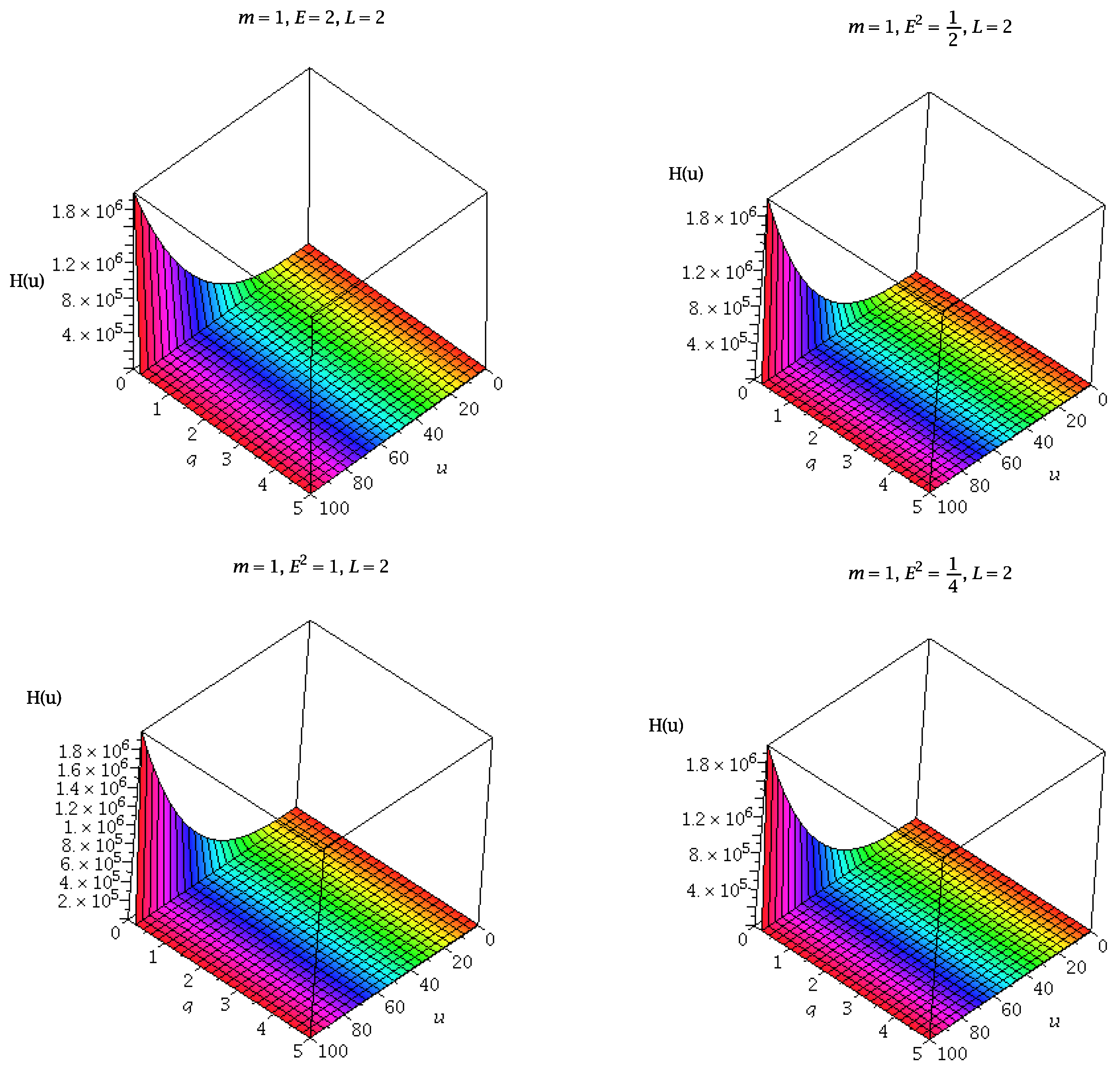
The function has been plotted for various values of E in Figure 9.
2.2. Photon Orbits
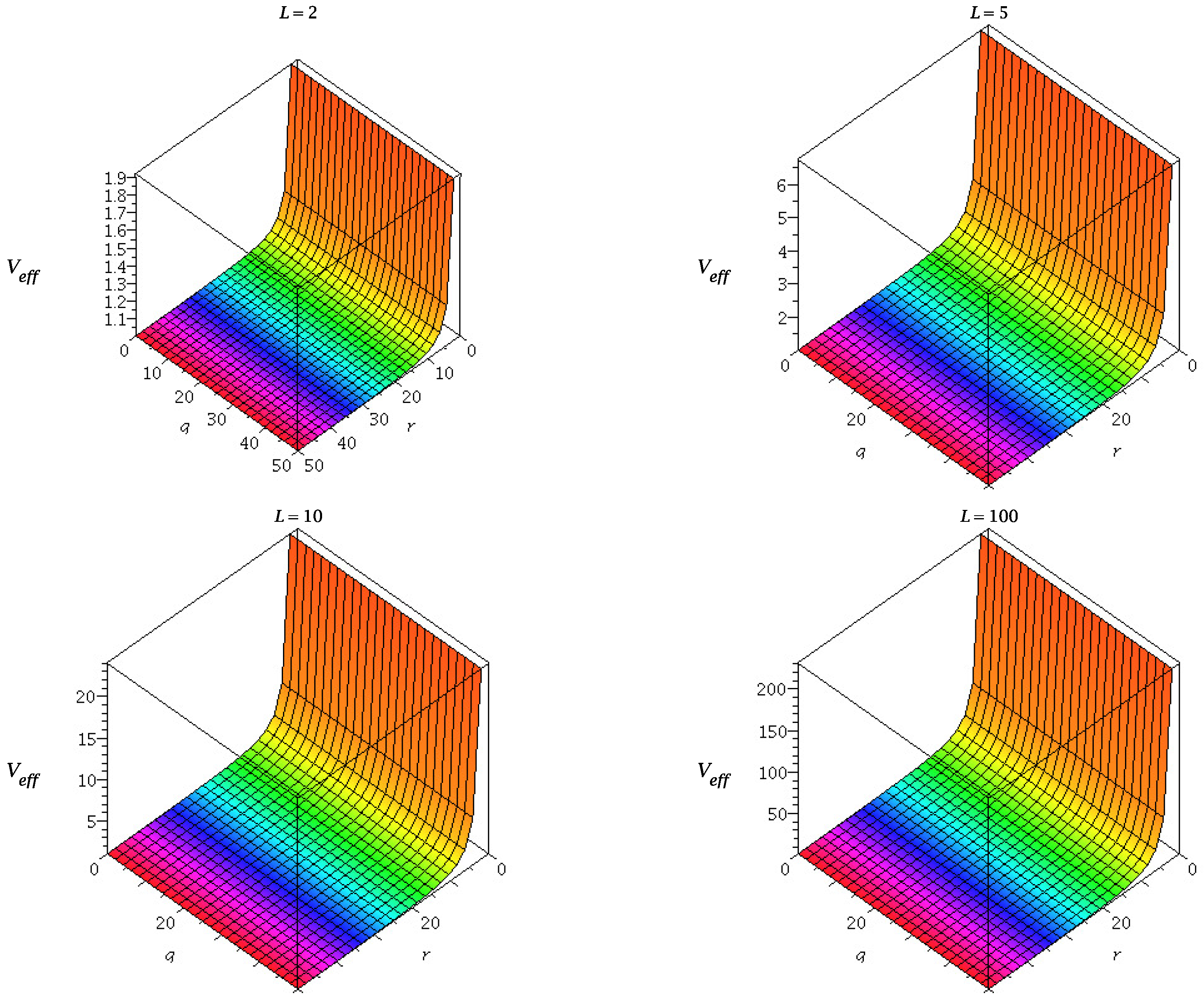
(i) The Effective Potential for Photon
For null geodesics [4], the effective potential becomes
Analogously, the geodesic motion of neutral test particles for photon could be studied by using the effective potential diagram which is plotted in Figure 10.
For circular null geodesics at , one obtains
and
Thus one could obtain the ratio of energy and angular momentum of the test particle evaluated at for CPO [4]
and,
Let be the impact parameter for null circular geodesics then
Let be the solution of Equation (40) which gives the radius of the photon orbit of the ABG space-time. In the limit , we recover the CPO of Schwarzschild BH which is .
(ii) The Null Geodesics using variable
For null geodesics the radial equation becomes
At the same time, we also consider the other relevant equations are
and
Similarly, by considering r as a function of , one derives the following equation
Now putting r by a new independent variable , one obtains
where b denotes the impact parameter. Differentiating this equation, one gets
which governs the light rays in ABG spacetime. Now the roots of Equation (46) could be determined by imposing the following condition
At , therefore we find the impact parameter as
When , one obtains the result of Schwarzschild BH when the root of could be obtained by solving the equation i.e.,
After solving this equation, we get the root . It is very easy to see the root of the Schwarzschild BH () when .
The light deflection could be calculated by using Equation (45). First we calculate the distance of closest approach by setting the condition which gives the value of b. Now substituting this values we get
It implies that the deflection of light depends upon the charge parameter.
(iii) The Radial Null Geodesics
Analogously, the radial null geodesics are derived to be
and
Thus one could find the following equation
Therefore the coordinate time is given by the following integral
It implies that when , the coordinate time goes to infinity as is expected. Now integrating Equation (52), one could get relation between the affine parameter time and the radial coordinates
This indicates that the affine parameter time is finite when the coordinate time is infinite.
3. Null Circular Geodesics and QNM for ABG Spacetime in the Eikonal Limit
In this section, we compute the QNM frequency for spherically symmetric ABG BH in the eikonal limit using the concept of Lyapunov exponent. It has been shown by Cardoso et al. [31] that there is a valid relation between null circular geodesics and QNM in the eikonal limit. Before proceed it we would shortly describe what is the QNM frequency? When a BH is perturbed it oscillates with a certain frequency, this frequency is called QNM frequency. It should be noted that unstable null circular geodesics could be used as a useful tool to describe the characteristic modes of a BH, which is so called the QNMs [32] frequency. In [33], we computed the QNM frequency for RN BH and Schwarzschild BH in the eikonal limit. To derive the QNM frequency for regular BH, We have borrowed the formula that has been derived by Cardoso et al. in [31] as
where n is denoted as the overtone number, ℓ is denoted as the angular momentum of the perturbation, is denoted as the angular frequency measured by the asymptotic observers and is denoted the coordinate time Lyapunov exponent for null circular geodesics which may be defined as in terms of the effective potential for null circular geodesics
and
For ABG BH the values of and are
and
Using these values and with Equation (59) one obtains the QNM frequency for ABG BH in the eikonal limit
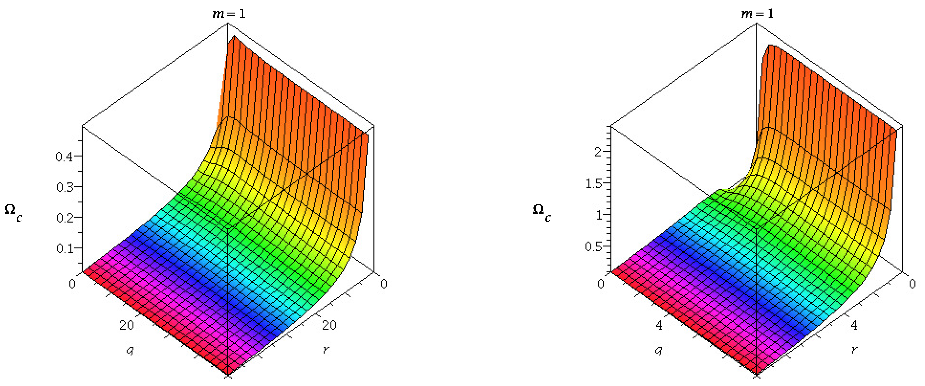
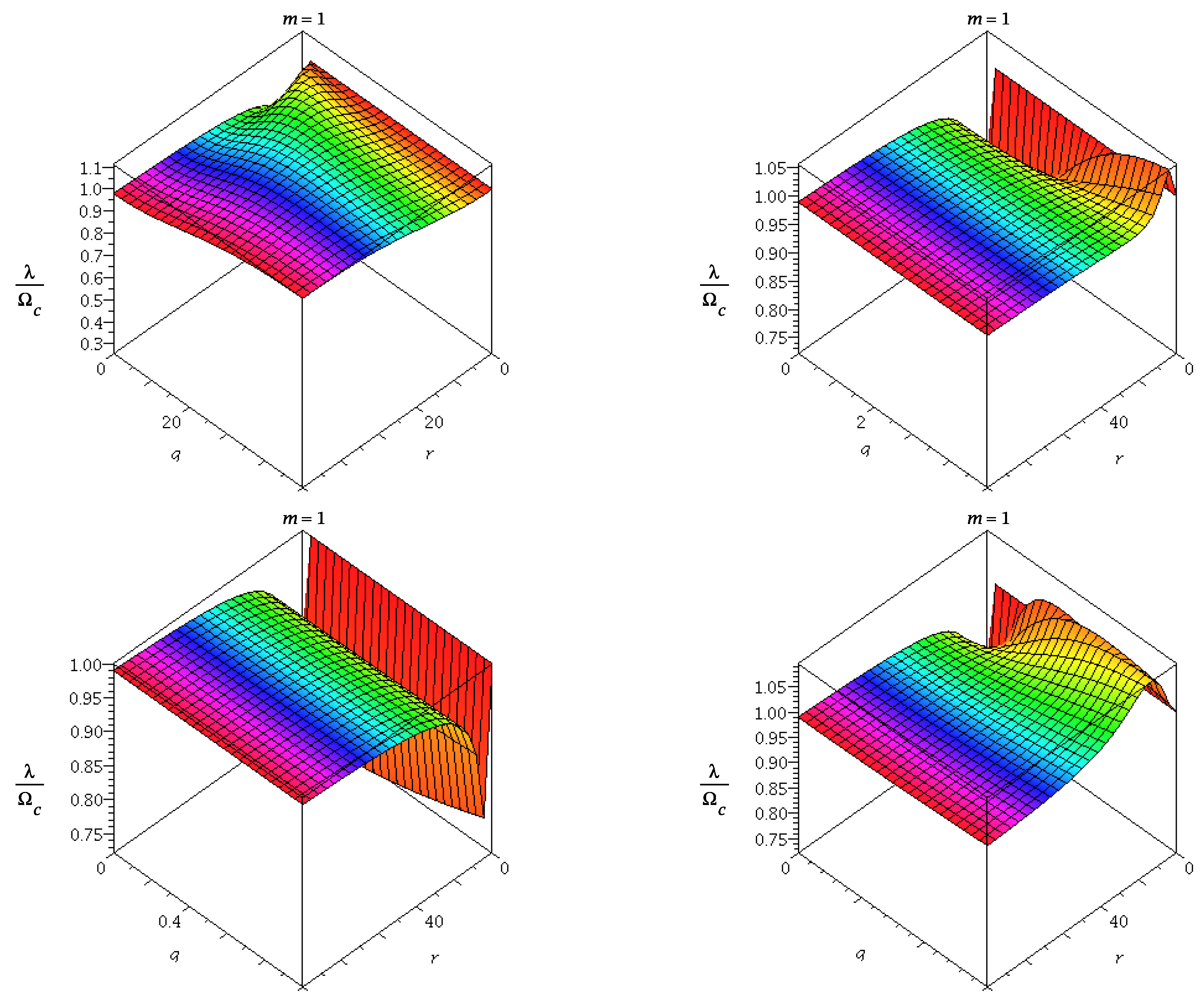
In the limit , one obtains the QNM frequency for Schwarzschild BH in the eikonal limit [33]. Similarly, it implies that the real and imaginary parts of the QNMs of regular ABG BH in the Eikonal limit are given by the frequency and instability time scale of the unstable circular photon geodesics. One could observe the variation of angular frequency and with and q in Figure 11, Figure 12 and Figure 13. It should be noted that in the eikonal limit the relation between the null circular geodesics and QNMs frequency get violated in case of higher curvature gravity i.e., Lovelock gravity [34] but for regular BHs this relation does not violate at all as we have seen from our computation.
4. CM Energy of the Collision Near the Horizon of the Ayón-Beato and García Space-Time
Now let us compute the CM energy for the collision of two neutral particles of same rest mass but different energy coming from infinity with and approaching the event horizon (infinite red-shift surface) of the ABG BH with different angular momenta and . Since our background is curved, so we need to define the CM frame properly. BSW [27] have been first derived the simple formula which is valid in both flat and curved spacetime
where and are the four velocity of the particles, properly normalized by (we have used the signature in the meric is (−+++)). This formula is of course well known in special relativity and in general relativity to ensure its validity.
Since the ABG space-time has also Killing symmetries followed by the Killing vector field thus energy and angular momentum (L) are conserved quantities as we have defined in case of Bardeen space-time. Therefore for massive particles of ABG space-time, the components of the four velocity are
and,
where
Substituting this in (63), we get the CM energy for ABG space-time
For simplicity, and putting the value of , we obtain the CM energy near the event horizon () of the ABG space-time
where is the root of the given equation in (7).
When we set , we get the CM energy of the Schwarzschild BH [35]
Since the spacetime is spherically symmetric therefore in this case the CM energy is finite in the region of the BH such that the angular momenta and of colliding particles are finite. This BH can acts as particle accelerators when two test charged particles approaching the horizon and provided that one of the test charge particle has critical value. This is discussed briefly in the Appendix section.
5. Summary and Conclusions
In this work, we examined the complete geodesic structure of a spherically symmetric, static charged Ayón-Beato and García BH. We also studied the properties of equatorial circular geodesic motion of neutral test particle by extremization of the effective potential for time-like circular orbits and null circular orbits. We particularly emphasized on the ISCO, MBCO and CPO of these regular BHs. These orbits are useful to extract the information about the back ground geometry and they are also relevant to the different kind of astrophysical procecess. We also studied an important feature of regular BHs that at a particular radius (say for RN BH, ), there exist zero angular momentum orbits due to the repulsive gravity. Using the geodesic properties of time-like particle, we derived the pseudo-Newtonian potential so called Paczyński-Witta Potential for ABG BH which are very important tools for analyzing the accretion-disk properties.
Next we computed the QNM frequency for these BHs by introducing the idea of Lyapunov exponent. By computing Lyapunov exponent we showed the QNM frequency of the regular BH can be expressed in terms of the parameters of the null CPO. We also showed that the real and imaginary parts of the QNM frequency of these regular BH could be expressed in terms of the instability time scale of the null CPO.
Moreover, we demonstrated that the collision of two neutral test particles falling freely from rest at infinity in the background of the regular ABG BH which is a regular BH space-time and singularity free solutions of the coupled system of a non-linear electrodynamics and general relativity. We have seen that the CM energy is finite and depends upon the fine tuning condition of the angular momentum parameter.
In the Appendix section, we investigated the collision of two charged test particles of different energy falling freely from rest at infinity in the background of the regular BHs and approaching to the horizon of the BH. Then there may be a possibility of this BH acts as particle accelerators while one of the charged test particle has critical value.
Conflicts of Interest
The authors declare not have any conflict of interest.
Appendix A
In this appendix section, we shall show the possibility of the CM energy is arbitrarily large for a regular BH when two charged particles of different energies are colliding and approaching to the horizon of the BH. We know the motion of a test particle of charge per unit mass describes in the BH geometry can be determined by the Lagrangian [1]
where is the electromagnetic gauge field1 and is the proper time. For example, we have considered the ABG metric in the equatorial plane then the Lagrangian becomes
The equations of motion can be easily written down from the Lagrangian
and
Taking these values and plugging back in Equation (63), one obtains the CM energy for ABG BH for two charged particles having charges and , and energies and
Now near the horizon say , the CM energy is calculated to be
Case I: When , one obtains the CM energy
There is a possibility of the CM energy to be infinite when one of the charge particle has critical value
where . For Reissner Nordström BH, this was derived by Zaslavskii [37].
Case II: When and , one obtains the CM energy in the following form
In this case, when one of the charge particle has critical value
Case III: When and , one finds the CM energy
In this case, also when one of the charge particle has critical value
Case IV: When and , one can obtain the CM energy
Here also , when one of the charge particle has critical value
Example: (a) For Reissner Nordström BH, the electromagnetic gauge field is therefore the critical charge is
it was derived in [37].
(b) For ABG BH, the potential function is calculated to be
and therefore the critical charge is computed to be
From the above calculation, we can conclude that the regular BH may act as particle accelerators when one of the charge particle has a critical charge.
References
- Chandrashekar, S. The Mathematical Theory of Black Holes; Clarendon Press: Oxford, UK, 1983. [Google Scholar]
- Hartle, J.B. Gravity-An Introduction To Einstein’s General Relativity; Benjamin Cummings: San Francisco, CA, USA, 2003. [Google Scholar]
- Shapiro, S.L.; Teukolsky, S.A. Black holes, White Dwarfs, and Neutron Stars: The Physics of Compact Objects; Wiley: New York, NY, USA, 1983. [Google Scholar]
- Pradhan, P. Regular Black Holes as Particle Accelerators. arXiv, 2014; arXiv:1402.2748. [Google Scholar]
- Pugliese, D.; Quevedo, H.; Ruffini, R. Circular motion of neutral test particles in Reissner-Nordström spacetime. Phys. Rev. D 2011, 83, 024021. [Google Scholar] [CrossRef]
- Fernando, S. Null Geodesics of Charged Black Holes in String Theory. Phys. Rev. D 2012, 85, 024033. [Google Scholar] [CrossRef]
- Pradhan, P.; Majumdar, P. Circular Orbits in Extremal Reissner Nordstrom Spacetimes. Phys. Lett. A 2011, 375, 474–475. [Google Scholar] [CrossRef]
- Bardeen, J. Non-singular general-relativistic gravitational collapse. In Proceedings of the Conference Proceedings in GR5, Tbilisi, Georgia, 9–13 September 1968; Tbilisi University Press: Tbilisi, Georgia, 1968. [Google Scholar]
- Ayón-Beato, E.; García, A. Regular black hole in general relativity coupled to nonlinear electrodynamics. Phys. Rev. Lett. 1998, 80, 5056. [Google Scholar] [CrossRef]
- Ayón-Beato, E.; García, A. The Bardeen Model as a Nonlinear Magnetic Monopole. Phys. Lett. B 2000, 493, 149–152. [Google Scholar] [CrossRef]
- Borde, A. Regular black holes and topology change. Phys. Rev. D 1997, 55, 7615. [Google Scholar] [CrossRef]
- Zhou, S.; Chen, J.; Wang, Y. Geodesic Structure of Test Particle in Bardeen Spacetime. Int. J. Mod. Phys. D 2011, 21, 1250077. [Google Scholar] [CrossRef]
- Ayón-Beato, E.; García, A. The Bardeen model as a nonlinear magnetic monopole. Phys. Lett. B 2000, 493, 149–152. [Google Scholar] [CrossRef] [Green Version]
- Ayón-Beato, E.; García, A. Nonsingular charged black hole solution for nonlinear source. Gen. Relativ. Gravit. 1999, 629, 629–633. [Google Scholar] [CrossRef]
- Ayón-Beato, E.; García, A. Four parametric regular black hole solution. Gen. Relativ. Gravit. 2005, 37, 635–641. [Google Scholar] [CrossRef]
- Ansoldi, S. Spherical black holes with regular center: A Review of existing models including a recent realization with Gaussian sources. arXiv, 2008; arXiv:0802.0330. [Google Scholar]
- Balart, L. Quasilocal Energy, Komar Charge and Horizon for Regular Black Holes. Phys. Lett. B 2010, 687, 280–285. [Google Scholar] [CrossRef]
- Bose, S.; Dadhich, N. On the Brown-York quasilocal energy, gravitational charge, and black hole horizons. Phys. Rev. D 1999, 60, 064010. [Google Scholar] [CrossRef]
- Bretón, N. Smarr’s formula for black holes with non-linear electrodynamics. Gen. Relativ. Gravit. 2005, 37, 643–650. [Google Scholar] [CrossRef]
- Balart, L.; Vagenas, E.C. Regular black hole metrics and the weak energy condition. Phys. Lett. B 2014, 730, 14–17. [Google Scholar] [CrossRef] [Green Version]
- García, A.; Hackmann, E.; Kunz, J.; Lämmerzahl, C.; Macías, A. Motion of test particles in a regular black hole space–time. J. Math. Phys. 2015, 56, 032501. [Google Scholar] [CrossRef]
- Eiroa, E.F.; Sendra, C.M. Gravitational lensing by a regular black hole. Class. Quantum Gravity 2011, 28, 085008. [Google Scholar] [CrossRef]
- Schee, J.; Stuchlík, Z. Gravitational lensing and ghost images in the regular Bardeen no-horizon spacetimes. J. Cosmol. Astropart. Phys. 2015, 2015, 48. [Google Scholar] [CrossRef]
- Toshmatov, B.; Abdujabbarov, A.; Stuchlík, Z.; Ahmedov, B. Quasinormal modes of test fields around regular black holes. Phys. Rev. D 2015, 91, 083008. [Google Scholar] [CrossRef]
- Paczyński, B.; Witta, P.J. Thick accretion disks and supercritical luminosities. Astron. Astrophys. 1980, 88, 23–31. [Google Scholar]
- Mukhopadhyay, B. Description of pseudo-Newtonian potential for the relativistic accretion disks around Kerr black hole. Astrophys J. 2002, 581, 427–430. [Google Scholar]
- Banados, M.; Silk, J.; West, S.M. Kerr Black Holes as Particle Accelerators to Arbitrarily High Energy. Phys. Rev. Lett. 2009, 103, 111102. [Google Scholar] [CrossRef] [PubMed]
- Stuchlík, Z.; Schee, J. Circular geodesic of Bardeen and Ayon-Beato-Garcia regular black-hole and no-horizon spacetimes. Int. J. Modern Phys. D 2015, 24, 1550020. [Google Scholar] [CrossRef]
- Bronnikov, K.A.; Fabris, J.C. Regular phantom black holes. Phys. Rev. Lett. 2006, 96, 251101. [Google Scholar] [CrossRef] [PubMed]
- Stuchlík, Z.; Hledík, S. Properties of the Reissner-Nordstrom spacetimes with a nonzero cosmological constant. Acta Phys. Slov. 2002, 52, 363–407. [Google Scholar]
- Cardoso, V.; Miranda, A.S.; Berti, E.; Witek, H.; Zanchin, V.T. Geodesic stability, Lyapunov exponents and quasinormal modes. Phys. Rev. D 2009, 79, 064016. [Google Scholar] [CrossRef]
- Konoplya, R.A.; Zhidenko, A. Quasinormal modes of black holes: From astrophysics to string theory. Rev. Mod. Phys. 2011, 83, 793–836. [Google Scholar] [CrossRef]
- Pradhan, P. Stability analysis and quasinormal modes of Reissner–Nordström space-time via Lyapunov exponent. Pramana-J. Phys. 2016, 87, 5. [Google Scholar] [CrossRef]
- Konoplya, R.A.; Stuchlík, Z. Are eikonal quasinormal modes linked to the unstable circular null geodesics? Phys. Lett. B 2017, 771, 597–602. [Google Scholar] [CrossRef]
- Baushev, A.N. Dark matter annihilation in the gravitational field of a black hole. Int. J. Mod. Phys. D 2009, 18, 1195. [Google Scholar] [CrossRef]
- Lemos, J.P.S.; Zanchin, V.T. New regular black hole solutions. AIP Conf. Proc. 2011, 1360, 145–150. [Google Scholar]
- Zaslavskii, O. Acceleration of particles by nonrotating charged black holes. JETP Lett. 2010, 92, 571–574. [Google Scholar] [CrossRef]
| 1. | The gauge field has the form . corresponds to the electric potential of regular BHs [36]. |
Figure 1.
The figure shows the variation of with r for different values of q.

Figure 2.
The figure depicts the variation of with r for different values of q.

Figure 3.
The figure depicts the variation of with r for various values of q. Here .
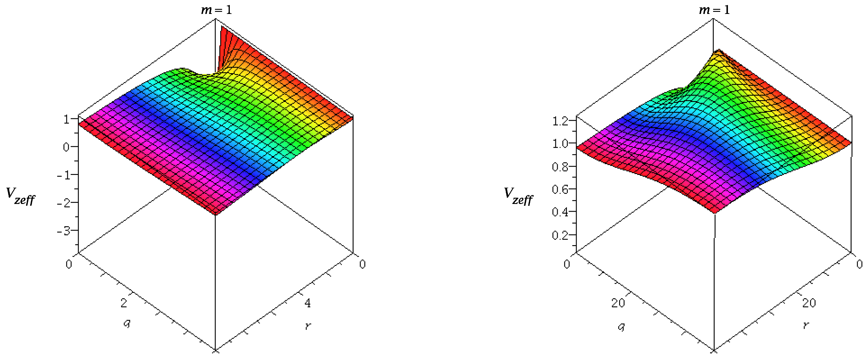
Figure 4.
The figure shows the variation of with r for ABG BH.

Figure 5.
The figure shows the variation of and with .

Figure 6.
The figure depicts the variation of with x and q for ABG BH.

Figure 7.
The figure depicts the variation of with x and q for ABG BH.
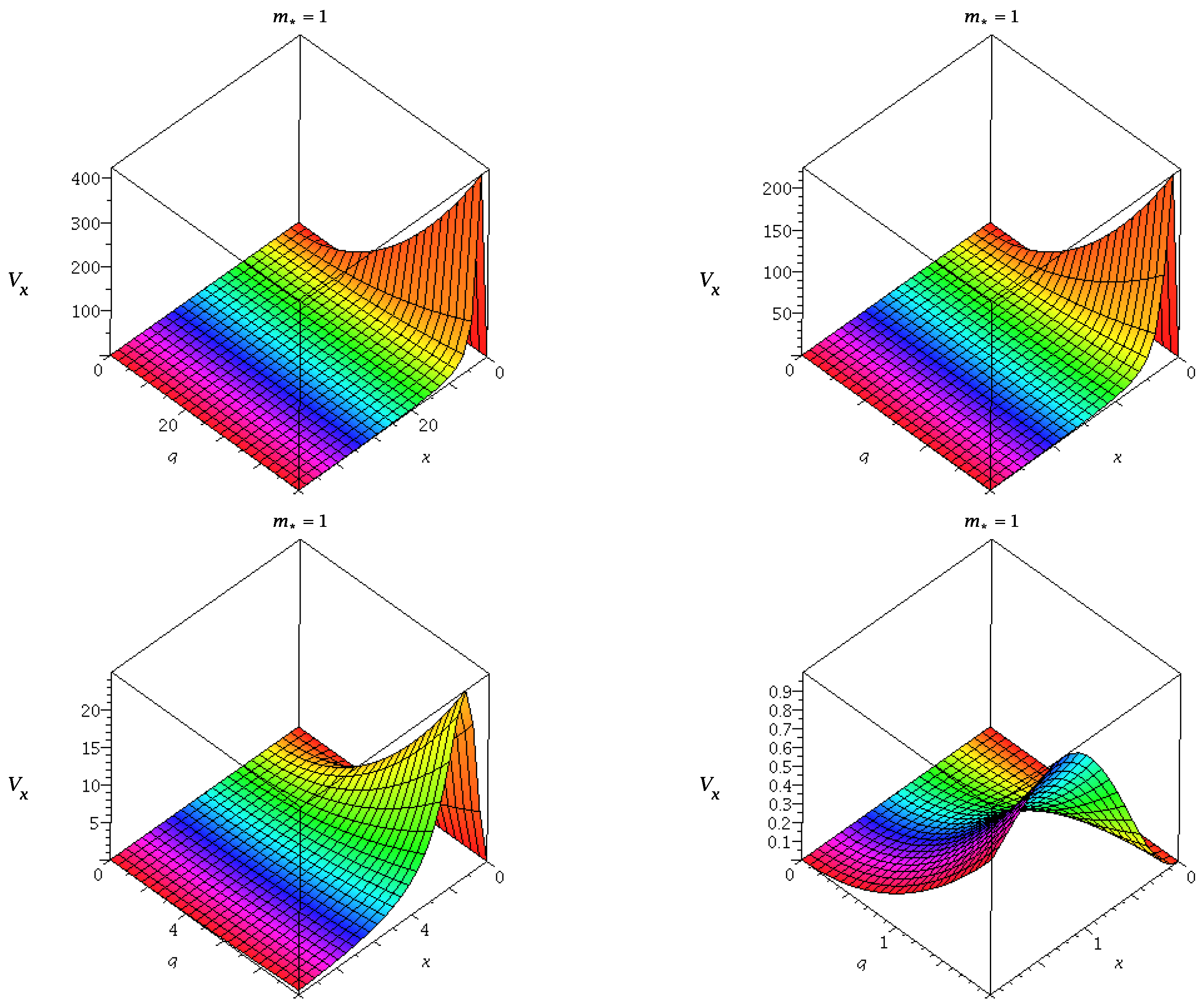
Figure 8.
The figure depicts the variation of with x and q for ABG BH.

Figure 9.
The figure demonstrates the variation of with u for ABG BH.

Figure 10.
The figure depicts the variation of with r for ABG BH.

Figure 11.
The figure shows the variation of with and q.

Figure 12.
The figure depitcs the variation of with and q for ABG BH.
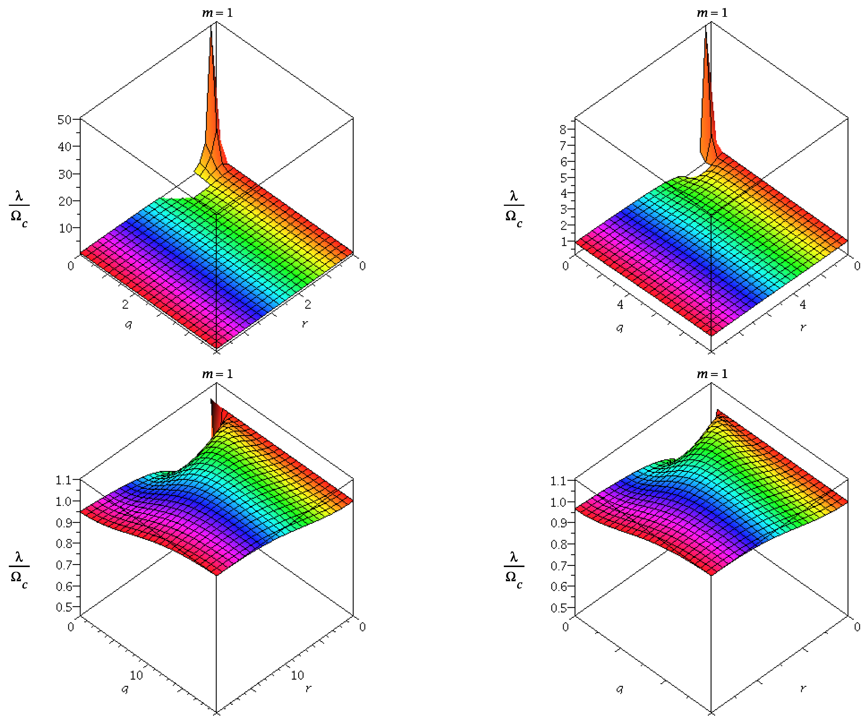
Figure 13.
The figure depitcs the variation of with and q for ABG BH.
© 2018 by the author. Licensee MDPI, Basel, Switzerland. This article is an open access article distributed under the terms and conditions of the Creative Commons Attribution (CC BY) license (http://creativecommons.org/licenses/by/4.0/).
Share and Cite
MDPI and ACS Style
Pradhan, P. Circular Geodesics, Paczyński-Witta Potential and QNMs in the Eikonal Limit for Ayón-Beato-García Black Hole. Universe 2018, 4, 55. https://doi.org/10.3390/universe4030055
AMA Style
Pradhan P. Circular Geodesics, Paczyński-Witta Potential and QNMs in the Eikonal Limit for Ayón-Beato-García Black Hole. Universe. 2018; 4(3):55. https://doi.org/10.3390/universe4030055
Chicago/Turabian StylePradhan, Parthapratim. 2018. "Circular Geodesics, Paczyński-Witta Potential and QNMs in the Eikonal Limit for Ayón-Beato-García Black Hole" Universe 4, no. 3: 55. https://doi.org/10.3390/universe4030055
Note that from the first issue of 2016, this journal uses article numbers instead of page numbers. See further details here.