Probing the Vacuum Decay Hypothesis with Growth Function Data

Abstract

In this paper, we present a method to probe the vacuum decay hypothesis by searching for deviations of the uncoupled dark matter density evolution formula. The method consists of expanding the dark matter density in a Taylor series and then comparing the series coefficients obtained from the observational analysis with its uncoupled values. We use the growth rate data to put constraints on the series coefficients. The results obtained are consistent with the $\mathrm{\Lambda }$CDM model, but it is shown that the possibility of vacuum decay cannot be ruled out by current growth rate data.

1. Introduction

Since observations of type Ia Supernovae (SNe Ia) revealed that the Universe is expanding at an accelerated rate [1,2], a wide variety of proposals has been put forward to explain such an unexpected discovery. In the context of general relativity, this observation can be explained if the fluid pervading the Universe violates the strong energy condition, i.e.,

$$\rho +3p<0.$$

(1)

This implies that the total pressure must be negative; since for matter (baryonic and dark) $p_m=0$ and for radiation $p_{\gamma }={\rho }_{\gamma }/3$, the Universe must also contain some unknown fluid with a pressure sufficiently negative to ensure the validity of (1). This additional component was dubbed dark energy. A universe dominated by a negative pressure fluid may be achieved if we add a cosmological term $\mathrm{\Lambda }$ to the Einstein field equations. The $\mathrm{\Lambda }-$term acts in the field equations like a fluid with a pressure $p_{\mathrm{\Lambda }}=-{\rho }_{\mathrm{\Lambda }}$, which can be associated with the zero point energy of all fields existing in the Universe [3,4]. Due to its simplicity and strong theoretical appeal, the cosmological constant (or vacuum energy) becomes the main candidate to explain the acceleration of the Universe. In fact, this vacuum-dominated model of the Universe, the so-called $\mathrm{\Lambda }$CDM model, has been favored by a large amount of observational data. Unfortunately, the value of the vacuum energy required to explain the present accelerated phase differs from the value predicted by the Quantum Field Theory (QFT) by at least 60 orders of magnitude [5] (see also [6] for a review). This huge discrepancy between theory and observation has challenged physicists’ imagination, and many proposals to solve this problem have appeared in the literature [7,8,9,10,11,12,13,14,15]. Since the QFT estimate of vacuum energy density is obtained in a flat space-time, the energy-momentum tensor in the Einstein equations should be zero since the Einstein tensor is zero in a flat space-time. Therefore, the vacuum energy density must be canceled by a bare cosmological constant. However, in curved space-time, it is expected that the vacuum contribution depends on the curvature, so that a renormalized vacuum energy density should be time dependent [16]. An evolving vacuum energy density is possible if vacuum energy is not conserved separately, but is coupled with the dark matter1 [22,23,24,25,26], i.e.,

$${\dot{\rho }}_{dm}+3H{\rho }_{dm}=-{\dot{\rho }}_{\mathrm{\Lambda }},$$

(2)

where ${\rho }_{dm}$ and ${\rho }_{\mathrm{\Lambda }}$ are the energy densities of dark matter and quantum vacuum, respectively, $H\equiv \dot{a}/a$ is the Hubble function and the dot denotes the time derivative. In order to solve the conservation Equation (2), it is common to guess specific functions for ${\rho }_{\mathrm{\Lambda }}$ or ${\rho }_{dm}$ (see, e.g., [27] for a list of vacuum decay models). Although seemingly arbitrary, most of these guesses have some physical motivation, and the diversity of vacuum decay scenarios existing in the literature is due to the diversity of aspects that we wish to study beyond the coupling itself. Obviously, such a diversity of decay models cannot provide a model-independent view of the vacuum decay hypothesis, significant insights can be obtained from some models such as, for instance, the Wang–Meng model [28], which assumes that the interaction between the dark fluids leads to a dilution of the dark matter density slower than the standard uncoupled one. Thus, clues of a possible vacuum decay can be found if the dark matter density evolution presents deviations from the separately-conserved case.

In this paper, a simple method to test the vacuum decay hypothesis is proposed. The approach is based on the series expansion method. In order to search for deviations from the separately-conserved case, the dark matter density is expanded in a power series. Since the interaction implies that ${\rho }_{dm}\ne {\rho }_{dm,0}{(1+z)}^3$, the series coefficients should present deviations from the uncoupled case. In order to search for these deviations, the growth rate data are used. Since no specific interaction model is assumed, this approach provides completely general results that must be satisfied by any reliable vacuum decay model.

This paper is organized as follows: in Section 2, the basic equations employed in the analysis are developed. In Section 3, the constraints on the parameters that quantify the deviations from the standard uncoupled dark matter density evolution equation are obtained from current growth rate data. Section 4 contains the conclusions and final comments.

2. The Method

Let us start expanding the dark matter density in a Taylor series around the redshift $z=0$,

$${\rho }_{dm}\left(z\right)={\rho }_{dm}{|}_{z=0}+\frac{d{\rho }_{dm}}{dz}{|}_{z=0}z+\frac{1}{2}\frac{d^2{\rho }_{dm}}{d{z}^2}{|}_{z=0}{z}^2+\frac{1}{6}\frac{d^3{\rho }_{dm}}{d{z}^3}{|}_{z=0}{z}^3+\frac{1}{24}\frac{d^4{\rho }_{dm}}{d{z}^4}{|}_{z=0}{z}^4+\cdots .$$

(3)

If dark matter and vacuum energy are separately conserved, the series coefficient are:

$$\begin{array}{c}\hfill \left\{\begin{array}{cc}\frac{d{\rho }_{dm}}{dz}{|}_{z=0}=3{\rho }_{dm,0},\hfill & \frac{1}{2}\frac{d^2{\rho }_{dm}}{d{z}^2}{|}_{z=0}=3{\rho }_{dm,0},\hfill \\ \hfill \frac{1}{6}\frac{d^3{\rho }_{dm}}{d{z}^3}{|}_{z=0}={\rho }_{dm,0},& \frac{1}{n!}\frac{d^n{\rho }_{dm}}{d{z}^n}{|}_{z=0}=0(\mathrm{if}n\ge 4).\end{array}\right.\end{array}$$

(4)

However, if the dark matter density is not conserved separately, deviations from the values in (4) should be observed. The following analysis is restricted to the third-order approximation. There are two reasons for this. The first one is that the third-order approximation contains the minimum number of terms required to get the uncoupled case as a special case. The second one is that, even if the dark fluids interact, the contribution of terms at orders higher than three must be negligible, at least in the redshift range covered by the available observational data. Otherwise, the $\mathrm{\Lambda }$CDM model, which assumes that the dark matter density is a third-order polynomial, would be unable to provide a good description of the observed Universe. Thus, to detect a possible interaction in the dark sector, it is sufficient to restrict our attention up to the third order terms.

In order to make the comparison between the uncoupled and coupled cases clearer, it is useful to rewrite the series coefficients as:

$$\begin{array}{c}\hfill \left\{\begin{array}{c}\frac{d{\rho }_{dm}}{dz}{|}_{z=0}\equiv 3({\rho }_{dm,0}+{\rho }_{1,0});\hfill \\ \hfill \frac{1}{2}\frac{d^2{\rho }_{dm}}{d{z}^2}{|}_{z=0}\equiv 3({\rho }_{dm,0}+{\rho }_{2,0});\\ \frac{1}{6}\frac{d^3{\rho }_{dm}}{d{z}^3}{|}_{z=0}\equiv {\rho }_{dm,0}+{\rho }_{3,0},\hfill \end{array}\right.\end{array}$$

(5)

where ${\rho }_{i,0}$ ($i=1,2,3$) are constants with the same dimensions as ${\rho }_{dm}$, which quantify the deviation from the uncoupled case. In terms of these new constants, the power series (3) becomes,

$$\begin{array}{c}\hfill {\rho }_{dm}\left(z\right)={\rho }_{dm,0}{(1+z)}^3+3{\rho }_{1,0}z+3{\rho }_{2,0}{z}^2+{\rho }_{3,0}{z}^3.\end{array}$$

(6)

Thus, clues of a possible vacuum decay can be found if any ${\rho }_{i,0}\ne 0$. There are two ways to search for values of ${\rho }_{i,0}\ne 0$. The first is to take also a third order approximation for ${\rho }_{\mathrm{\Lambda }}$ and to use the conservation Equation (2) to relate the series coefficients of ${\rho }_{\mathrm{\Lambda }}$ with the series coefficients of ${\rho }_{dm}$. The second one is to substitute Equation (6) into Equation (2) and to solve it directly to obtain ${\rho }_{\mathrm{\Lambda }}$. Here, we will follow these two routes.

2.1. Approach I

The starting point is performing a third order Taylor approximation for the vacuum energy density,

$${\rho }_{\mathrm{\Lambda }}\left(z\right)={\rho }_{\mathrm{\Lambda }}{|}_{z=0}+\frac{d{\rho }_{\mathrm{\Lambda }}}{dz}{|}_{z=0}z+\frac{1}{2}\frac{d^2{\rho }_{\mathrm{\Lambda }}}{d{z}^2}{|}_{z=0}{z}^2+\frac{1}{6}\frac{d^3{\rho }_{\mathrm{\Lambda }}}{d{z}^3}{|}_{z=0}{z}^3.$$

(7)

Then, we rewrite (2) in terms of the redshift, i.e.,

$$\frac{d{\rho }_{\mathrm{\Lambda }}}{dz}=-\frac{d{\rho }_{dm}}{dz}+3\frac{{\rho }_{dm}}{1+z}$$

(8)

and use the above equation as a recurrence formula to write the derivatives of ${\rho }_{\mathrm{\Lambda }}$ at $z=0$ in terms of ${\rho }_{dm}$ derivatives, so that:

$$\begin{array}{c}\left\{\begin{array}{c}\frac{d^{}{\rho }_{\mathrm{\Lambda }}}{d{z}^{}}{|}_{z=0}=-\frac{d{\rho }_{dm}}{dz}{|}_{z=0}+3{\rho }_{m,0}\hfill \\ \frac{d^2{\rho }_{\mathrm{\Lambda }}}{d{z}^2}{|}_{z=0}=-\frac{d^2{\rho }_{dm}}{d{z}^2}{|}_{z=0}+3\frac{d{\rho }_{dm}}{dz}{|}_{z=0}-3{\rho }_{m,0}\hfill \\ \frac{d^3{\rho }_{\mathrm{\Lambda }}}{d{z}^3}{|}_{z=0}=-\frac{d^3{\rho }_{dm}}{d{z}^3}{|}_{z=0}+3\frac{d^2{\rho }_{dm}}{d{z}^2}{|}_{z=0}-6\frac{d{\rho }_{dm}}{dz}{|}_{z=0}+6{\rho }_{m,0}.\hfill \end{array}\right.\hfill \end{array}$$

(9)

From Equation (6), we get:

$$\begin{array}{c}\left\{\begin{array}{c}\frac{d^{}{\rho }_{\mathrm{\Lambda }}}{d{z}^{}}{|}_{z=0}=-3{\rho }_{1,0}\hfill \\ \frac{d^2{\rho }_{\mathrm{\Lambda }}}{d{z}^2}{|}_{z=0}=9{\rho }_{1,0}-6{\rho }_{2,0}\hfill \\ \frac{d^3{\rho }_{\mathrm{\Lambda }}}{d{z}^3}{|}_{z=0}=-18{\rho }_{1,0}+18{\rho }_{2,0}-6{\rho }_{3,0}.\hfill \end{array}\right.\hfill \end{array}$$

(10)

Finally, replacing the above coefficients in the series (7) and performing a bit of algebra to write ${\rho }_{\mathrm{\Lambda }}$ in terms of powers of $1+z$, we have:

$$\begin{array}{ccc}\hfill {\rho }_{\mathrm{\Lambda }}\left(z\right)& =& {\rho }_{\mathrm{\Lambda },0}-3{\rho }_{1,0}z-3{\rho }_{2,0}{z}^2-{\rho }_{3,0}{z}^3+3({\rho }_{2,0}-{\rho }_{1,0}){(1+z)}^3\hfill \\ & +& \frac{9}{2}(3{\rho }_{1,0}-2{\rho }_{2,0}){(1+z)}^2+9({\rho }_{2,0}-2{\rho }_{1,0})(1+z)+\frac{3}{2}(5{\rho }_{1,0}-2{\rho }_{2,0}).\hfill \end{array}$$

(11)

Since we are assuming that the baryonic matter density is conserved separately, i.e., ${\rho }_b\left(z\right)={\rho }_{b,0}{(1+z)}^3$, the Friedmann equation takes the form:

$$\begin{array}{c}\hfill H_{\mathrm{I}}^2={\left(\frac{\dot{a}}{a}\right)}^2=H_{\mathrm{\Lambda }\mathrm{CDM}}^2+\Delta H_{\mathrm{I}}^2\end{array}$$

(12)

where:

$$H_{\mathrm{\Lambda }\mathrm{CDM}}^2\equiv H_0^2\left[{\mathrm{\Omega }}_{\gamma ,0}{(1+z)}^4+{\mathrm{\Omega }}_{m,0}{(1+z)}^3+{\mathrm{\Omega }}_{k,0}{(1+z)}^2+{\mathrm{\Omega }}_{\mathrm{\Lambda },0}\right]$$

(13)

is the Friedmann equation for the $\mathrm{\Lambda }$CDM model and:

$$\begin{array}{ccc}\hfill \Delta H_{\mathrm{I}}^2& \equiv & H_0^2[3({\mathrm{\Omega }}_{2,0}-{\mathrm{\Omega }}_{1,0}){(1+z)}^3+\frac{9}{2}(3{\mathrm{\Omega }}_{1,0}-2{\mathrm{\Omega }}_{2,0}){(1+z)}^2\hfill \\ & +& 9({\mathrm{\Omega }}_{2,0}-2{\mathrm{\Omega }}_{1,0})(1+z)+\frac{3}{2}(5{\mathrm{\Omega }}_{1,0}-2{\mathrm{\Omega }}_{2,0})].\hfill \end{array}$$

(14)

is the deviation from the $\mathrm{\Lambda }$CDM model caused by a possible interaction between dark matter and vacuum energy in this approach. In the above equations, ${\mathrm{\Omega }}_{\gamma ,0}={\rho }_{\gamma ,0}/{\rho }_{c,0}$, ${\mathrm{\Omega }}_{m,0}={\rho }_{m,0}/{\rho }_{c,0}$ and ${\mathrm{\Omega }}_{\mathrm{\Lambda },0}={\rho }_{\mathrm{\Lambda },0}/{\rho }_{c,0}$ are, respectively, the density parameters of radiation, matter (baryonic plus dark) and quantum vacuum, ${\mathrm{\Omega }}_{k,0}=-k{c}^2/{\left(a_0{H}_0\right)}^2$ is the curvature parameter and ${\mathrm{\Omega }}_{i,0}={\rho }_{i,0}/{\rho }_{c,0}$ ($i=1,2,3$) with ${\rho }_{c,0}=3H_0^2{c}^2/8\pi G$. It is interesting to note that the parameter ${\mathrm{\Omega }}_{3,0}$ does not appear in the Friedmann equation.

2.2. Approach II

Now, substituting (6) in the continuity Equation (2) (or equivalently, Equation (8)), it is found, after integration and some algebraic manipulations, that the vacuum energy density evolves as:

$$\begin{array}{ccc}\hfill {\rho }_{\mathrm{\Lambda }}\left(z\right)& =& {\rho }_{\mathrm{\Lambda },0}-3{\rho }_{1,0}z-3{\rho }_{2,0}{z}^2-{\rho }_{3,0}{z}^3+9({\rho }_{1,0}-2{\rho }_{2,0}+{\rho }_{3,0})(1+z)+\frac{9}{2}({\rho }_{2,0}-{\rho }_{3,0}){(1+z)}^2\hfill \\ & +& {\rho }_{3,0}{(1+z)}^3-3(3{\rho }_{1,0}-3{\rho }_{2,0}+{\rho }_{3,0})ln(1+z)-\frac{1}{2}(18{\rho }_{1,0}-27{\rho }_{2,0}+11{\rho }_{3,0}).\hfill \end{array}$$

(15)

By following this approach, the Friedmann equation takes the form:

$$\begin{array}{c}\hfill H_{\mathrm{II}}^2=H_{\mathrm{\Lambda }\mathrm{CDM}}^2+\Delta H_{\mathrm{II}}^2\end{array}$$

(16)

where:

$$\begin{array}{ccc}\hfill \Delta H_{\mathrm{II}}^2& \equiv & H_0^2[9({\mathrm{\Omega }}_{1,0}-2{\mathrm{\Omega }}_{2,0}+{\mathrm{\Omega }}_{3,0})(1+z)+\frac{9}{2}({\mathrm{\Omega }}_{2,0}-{\mathrm{\Omega }}_{3,0}){(1+z)}^2+{\mathrm{\Omega }}_{3,0}{(1+z)}^3\hfill \\ & -& 3(3{\mathrm{\Omega }}_{1,0}-3{\mathrm{\Omega }}_{2,0}+{\mathrm{\Omega }}_{3,0})ln(1+z)-\frac{1}{2}(18{\mathrm{\Omega }}_{1,0}-27{\mathrm{\Omega }}_{2,0}+11{\mathrm{\Omega }}_{3,0})]\hfill \end{array}$$

(17)

is the deviation from the $\mathrm{\Lambda }$CDM due to the interaction between dark fluids in this new scenario. Note that the perturbations in the $\mathrm{\Lambda }$CDM model will depend on the route followed. Furthermore, note that terms that evolve like cosmic strings, ${(1+z)}^2$, and domain wall, $(1+z)$, arise naturally in the Friedmann equation if vacuum decay is allowed. Motivated by the recent results of thecosmic microwave background (CMB) power spectrum [29,30,31,32], we assume spatial flatness in the following analyses.

3. Observational Constraints

3.1. Dark Energy Equivalence

Before we proceed with the observational analysis, it must be stressed that the Hubble functions (12) and (16) can be equivalently obtained from dark energy models. This can be seen by remembering that for a dark energy fluid, the parameter of the equation of state, neglecting the contributions of curvature and radiation, can be written as:

$$\begin{array}{c}\hfill w=\frac{1}{3}\frac{2(1+z)\eta {\eta }^{\prime }-3{\eta }^2}{{\eta }^2-{\mathrm{\Omega }}_{m,0}{(1+z)}^3},\end{array}$$

(18)

where $\eta =H/H_0$, and the prime denotes a differentiation with respect to z. This implies that from geometric probes as, for instance, SN Ia distance and baryon acoustic oscillation (BAO) measurements, it is impossible to distinguish between dark energy and vacuum decay scenarios, at least looking only at deviations in the standard dark matter density formula. Therefore, to avoid misleading conclusions, we use the growth rate data, which depend on the matter density expression.

3.2. Growth Function

In the linear regime, the matter density perturbations $\delta =\delta {\rho }_m/{\rho }_m$ for dynamical vacuum models satisfy2 [34]:

$$\ddot{\delta }+(2H-\gamma )\dot{\delta }-(2H\gamma +\dot{\gamma }+4\pi G{\rho }_m)\delta =0,$$

(19)

where $\gamma =\dot{{\rho }_{\mathrm{\Lambda }}}/{\rho }_m$ and G is the Newton constant. By defining the growth factor $f\equiv dln\delta /lna$, this second order time differential equation is reduced to:

$$f^{\prime }+f^2+\left(1-q-\frac{\gamma }{H}\right)f-2\frac{\gamma }{H}-\frac{\dot{\gamma }}{H^2}-\frac{3}{2}{\mathrm{\Omega }}_m=0,$$

(20)

where $f^{\prime }=df/dlna$, $q=-\ddot{a}/\left(a{H}^2\right)$ is the deceleration parameter and:

$${\mathrm{\Omega }}_m=\frac{1}{{\eta }_{I\left(II\right)}^2}\left[{\mathrm{\Omega }}_{m,0}{a}^{-3}+3{\mathrm{\Omega }}_{1,0}\left(\frac{1}{a}-1\right)+3{\mathrm{\Omega }}_{2,0}{\left(\frac{1}{a}-1\right)}^2+{\mathrm{\Omega }}_{3,0}{\left(\frac{1}{a}-1\right)}^3\right],$$

(21)

with ${\eta }_{I\left(II\right)}\equiv H_{I\left(II\right)}/H_0$.

3.3. Constraints

In order to discuss the observational constraints on the parameters ${\mathrm{\Omega }}_{1,0}$, ${\mathrm{\Omega }}_{2,0}$ and ${\mathrm{\Omega }}_{3,0}$, we use the data listed in

Table 1. Currently available data for growth rates used here.

z	f	${\mathit{\sigma }}_{\mathit{f}}$	Ref.
0.15	0.49	0.14	[36]
0.15	0.51	0.11	[37,38]
0.22	0.60	0.10	[39]
0.32	0.654	0.18	[40]
0.34	0.64	0.09	[41]
0.35	0.70	0.18	[42]
0.41	0.70	007	[39]
0.42	0.73	0.09	[43]
0.55	0.75	0.18	[44]
0.59	0.75	0.09	[43]
0.60	0.73	0.07	[39]
0.77	0.91	0.36	[36]
0.78	0.70	0.08	[39]
1.4	0.90	0.24	[45]
2.125	0.78	0.24	[46]
2.72	0.78	0.24	[46]
3.0	0.99	0.24	[47]

, which were obtained from the redshift distortion parameter $\beta =f/b$ (b is the bias) measurements or from power spectrum amplitudes of Lyman-$\alpha$ forest data (see the original references listed in Table 1 for more details). Thus, in the present analyses, we minimize the function:

$${\chi }^2=\sum _{i=1}^{17}\frac{{(f_i^{obs}-f_i^{theo})}^2}{{\sigma }_i^2},$$

(22)

where $f_i^{obs}$ is the observed value of the growth function at redshift $z_i$, ${\sigma }_i$ its uncertainty and $f_i^{theo}$ the value of $f\left(z_i\right)$ provided theoretically. In agreement with recent studies involving SN Ia, (BAO), CMB and $H_0$[35], we also add the constraint ${\mathrm{\Omega }}_{m,0}=0.303\pm 0.007$.

In order to obtain $f_i^{theo}$, we solve the differential Equation (20) by treating the initial condition $f_0$ as a nuisance parameter and marginalizing over $f_0$.

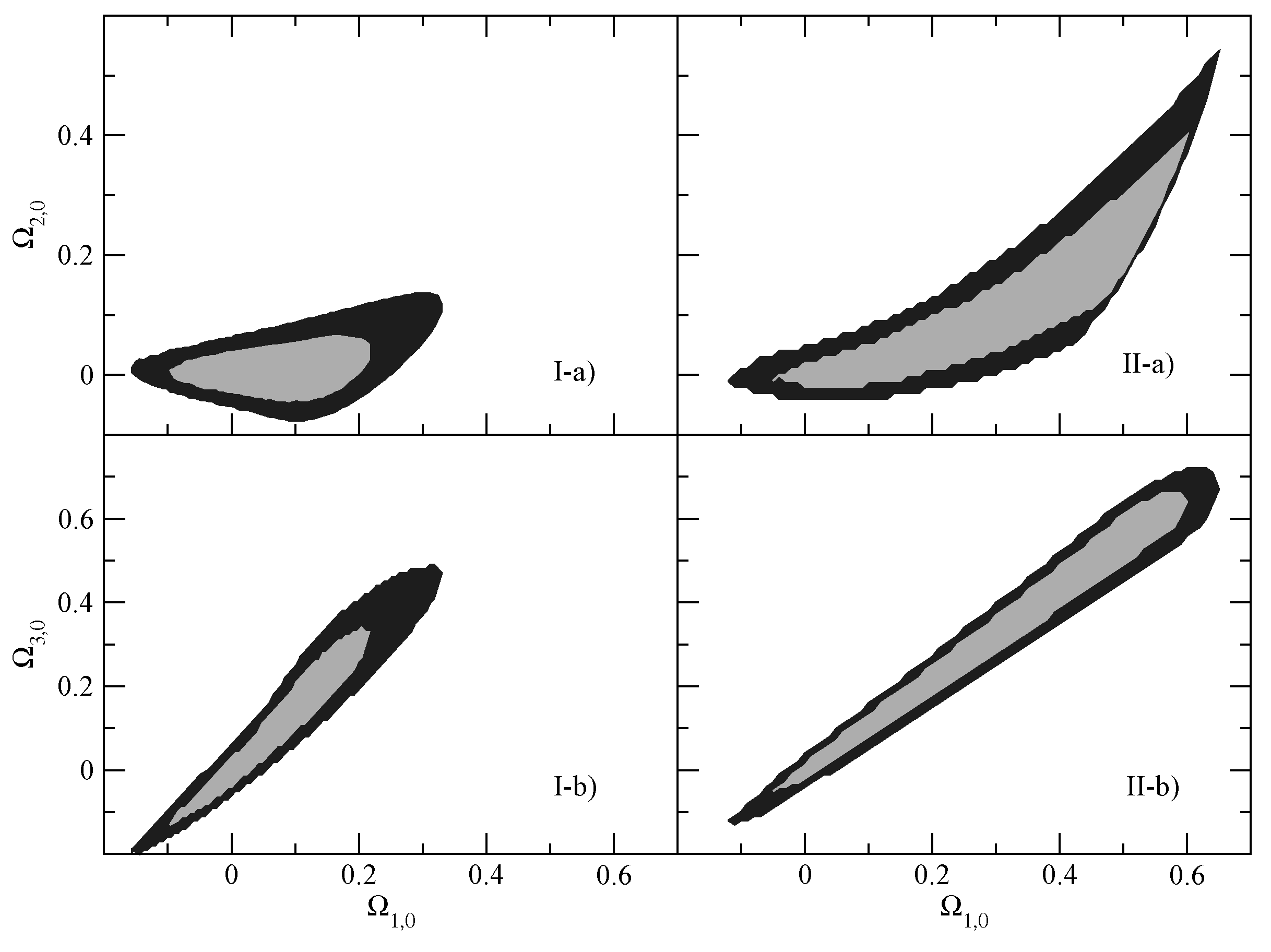
Figure 1 shows the results of the statistical analysis at $68\%$ and $95\%$ confidence levels. Panels I-a) and II-a) of Figure 1 shows the ${\mathrm{\Omega }}_{1,0}-{\mathrm{\Omega }}_{2,0}$ parametric space obtained from Approaches I and II, respectively, by marginalizing over ${\mathrm{\Omega }}_{3,0}$, while panels I-b) and II-b) of Figure 1 shows the ${\mathrm{\Omega }}_{1,0}-{\mathrm{\Omega }}_{3,0}$ parametric space obtained, respectively, from Approaches I and II by marginalizing over ${\mathrm{\Omega }}_{2,0}$. For the sake of comparison, the same scale is used for both approaches. The best fit values are indicated in

Table 2. The best fit values for ${\mathrm{\Omega }}_{1,0}$, ${\mathrm{\Omega }}_{2,0}$ and ${\mathrm{\Omega }}_{3,0}$. The upper and lower limits stand for $2\sigma$ errors.

	${\mathbf{\Omega }}_{1,0}$	${\mathbf{\Omega }}_{2,0}$	${\mathbf{\Omega }}_{3,0}$	${\mathit{\chi }}_{\mathit{min}}^2$
Approach I	$-{0.072}_{-0.198}^{+0.198}$	${0.004}_{-0.064}^{+0.088}$	${0.10}_{-0.27}^{+0.31}$	1.941
Approach II	${0.33}_{-0.41}^{+0.29}$	${0.11}_{-0.14}^{+0.36}$	${0.36}_{-0.46}^{+0.33}$	1.285
$\mathrm{\Lambda }$CDM model	0	0	0	2.857

, which also displays ${\chi }_{min}^2$ for the $\mathrm{\Lambda }$CDM model. These results are clearly compatible with the $\mathrm{\Lambda }$CDM model (${\mathrm{\Omega }}_{1,0}={\mathrm{\Omega }}_{2,0}={\mathrm{\Omega }}_{3,0}=0$). However, a simple inspection of Figure 1 shows that the vacuum decaying hypothesis cannot be excluded since, in both approaches, there is enough space for interacting models. Note that the shape of the corresponding parametric spaces are very similar for both approaches. However, Approach II is less restrictive than Approach I. This can be due the integration process, which increases the degeneracy between the parameters.

Due to its generality and less restrictive character, the method presented in this paper provides a fast and easy way to make (over)estimates of the values of the free parameters of many vacuum decaying models with a smooth analytical function. For instance, for the Wang–Meng model,

$${\rho }_{dm}={\rho }_{dm,0}{(1+z)}^{3-ϵ},$$

(23)

the parameter $ϵ$ is related to the parameters ${\mathrm{\Omega }}_{1,0}$, ${\mathrm{\Omega }}_{2,0}$ and ${\mathrm{\Omega }}_{3,0}$ by:

$$ϵ+3\frac{{\mathrm{\Omega }}_{1,0}}{{\mathrm{\Omega }}_{dm,0}}=0,$$

(24)

$${ϵ}^2-5ϵ-6\frac{{\mathrm{\Omega }}_{2,0}}{{\mathrm{\Omega }}_{m,0}}=0$$

(25)

and:

$${ϵ}^3-4{ϵ}^2+ϵ-6\frac{{\mathrm{\Omega }}_{3,0}}{{\mathrm{\Omega }}_{m,0}}=0.$$

(26)

By taking the first of these relations and the results of Table 2, we obtain $-1.25<ϵ<2.67$ for Approach I and $-6.14<ϵ<0.79$ for Approach II. Both intervals cover the range provided for this parameter by recent research works [48,49,50].

Finally, for the sake of completeness, it is useful to study the evolution of the deceleration parameter. In the present analysis, it is easy to show that:

$$\begin{array}{c}\hfill q_{I\left(II\right)}\left(z\right)=\frac{H_{\mathrm{\Lambda }\mathrm{CDM}}^2{q}_{\mathrm{\Lambda }\mathrm{CDM}}+\Delta H_{I\left(II\right)}^2\Delta q_{I\left(II\right)}}{H_{I\left(II\right)}^2},\end{array}$$

(27)

where:

$$q_{\mathrm{\Lambda }\mathrm{CDM}}=-1+(1+z)\frac{1}{H_{\mathrm{\Lambda }\mathrm{CDM}}}\frac{d{H}_{\mathrm{\Lambda }\mathrm{CDM}}}{dz}$$

(28)

is the deceleration parameter for the $\mathrm{\Lambda }$CDM model and $\Delta q_{I\left(II\right)}$ is defined as:

$$\Delta q_{I\left(II\right)}\equiv -1+(1+z)\frac{1}{\Delta H_{I\left(II\right)}}\frac{d\Delta H_{I\left(II\right)}}{dz}.$$

(29)

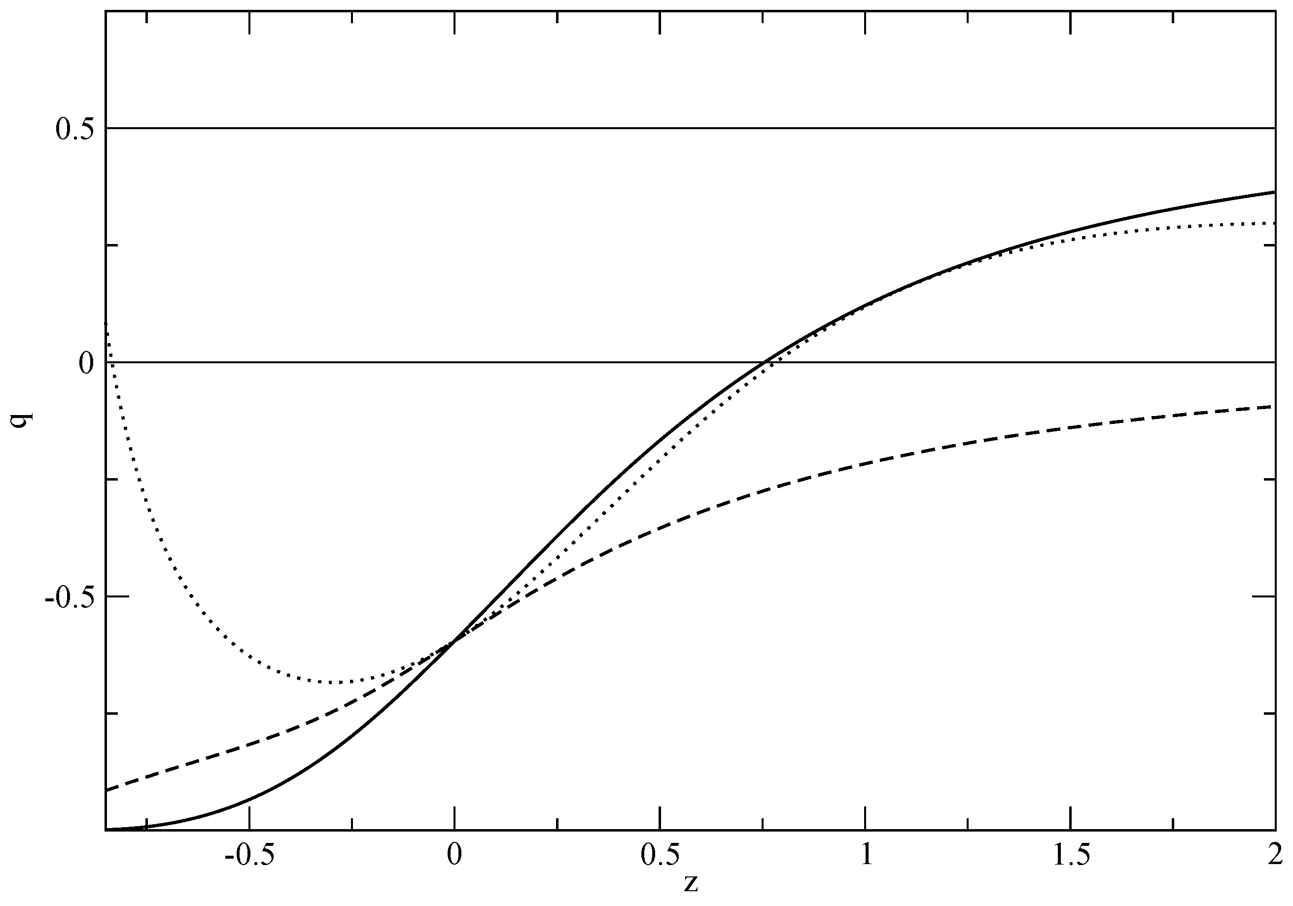
Figure 2 shows the deceleration parameter for the $\mathrm{\Lambda }$CDM model (solid line), for the best fit point from Approach I (dotted line) and for the best fit point from Approach II (dashed line). The deviation of the best fit points from the $\mathrm{\Lambda }$CDM is clear. The transition redshifts of the best fit of Approach I and the $\mathrm{\Lambda }$CDM model is near. However, an early accelerated Universe is compatible with the best fit points of Approach II. We observe that the best fit of Approach I produces an interacting scenario with the longest matter dominated era, marked by the $q=0.5$ line, and with a transient accelerated phase, in agreement with recent studies [51,52,53].

4. Final Remarks

In this paper, a way to probe the vacuum decaying hypothesis using a Taylor expansion of the dark matter density around the redshift $z=0$ was presented. If vacuum decay is allowed, the series will not converge to the simple third-order polynomial ${\rho }_{dm}={\rho }_{dm,0}{(1+z)}^3$. Thus, an efficient and completely general method of probing the vacuum decaying hypothesis is to search for deviations of the series coefficients of the values provided by the uncoupled case. We note that from geometric probes as SNe Ia, BAO and CMB, it is impossible to distinguish between quintessence and vacuum decay scenarios searching only for deviations in the standard dark matter density evolution. Thus, we perform an observational search for such deviations using 17 growth function measurements collected from several references. Since the growth function depends on the matter density expression, these data should be sensitive to deviations in the standard dark matter density evolution, allowing detection of a vacuum decay. The results obtained are compatible with the $\mathrm{\Lambda }$CDM model. However, at least with the data currently available, it is not possible to rule out the vacuum decaying models. We claim that the method presented here may prove very useful to detect a possible vacuum decay in the future when a larger amount of growth function data with a greater accuracy become available.

References

- Riess, A.G.; Filippenko, A.V.; Challis, P.; Clocchiattia, A.; Diercks, A.; Garnavich, P.M.; Gilliland, R.L.; Hogan, C.J.; Jha, S.; Kirshner, R.P.; et al. Observational Evidence from Supernovae for an Accelerating Universe and a Cosmological Constant. Astron. J. 1998, 116, 1009–1038. [Google Scholar] [CrossRef]
- Perlmutter, S.; Aldering, G.; Goldhaber, G.; Knop, R.A.; Nugent, P.; Castro, P.G.; Deustua, S.; Fabbro, S.; Goobar, A.; Groom, D.E. Measurements of Ω and Λ from 42 High-Redshift Supernovae. Astrophys. J. 1999, 517, 565–586. [Google Scholar] [CrossRef]
- Zeldovich, Y.B. Cosmological Constant and Elementary Particles. J. Exp. Theor. Phys. Lett. 1967, 6, 316. [Google Scholar] [CrossRef]
- Zeldovich, Y.B. The Cosmological constant and the theory of elementary particles. Sov. Phys. Uspekhi 1968, 11, 381–393. [Google Scholar] [CrossRef]
- Weinberg, S. The cosmological constant problem. Rev. Mod. Phys. 1989, 61, 1–24. [Google Scholar] [CrossRef]
- Bousso, R. TASI Lectures on the Cosmological Constant. Gen. Relativ. Gravit. 2008, 40, 607–637. [Google Scholar] [CrossRef]
- Emelyanov, V.; Klinkhamer, F.R. Possible solution to the main cosmological constant problem. Phys. Rev. D 2012, 85, 103508. [Google Scholar] [CrossRef]
- Shaw, D.J.; Barrow, J.D. The Value of the Cosmological Constant. Phys. Rev. D 2011, 83, 043518. [Google Scholar] [CrossRef]
- Barrow, J.D.; Shaw, D.J. A New Solution of The Cosmological Constant Problems. Phys. Rev. Lett. 2011, 106, 101302. [Google Scholar] [CrossRef] [PubMed]
- Aslanbeigi, S.; Robbers, G.; Foster, B.Z.; Kohri, K.; Afshordi, N. Phenomenology of gravitational aether as a solution to the old cosmological constant problem. Phys. Rev. D 2011, 84, 103522. [Google Scholar] [CrossRef]
- Mannheim, P.D. Comprehensive solution to the cosmological constant, zero-point energy, and quantum gravity problems. Gen. Rel. Grav. 2011, 43, 703–750. [Google Scholar] [CrossRef]
- Linde, A.; Vanchurin, V. Towards a non-anthropic solution to the cosmological constant problem. arXiv, 2010; arXiv:1011.0119. [Google Scholar]
- Stefancic, H. The solution of the cosmological constant problem from the inhomogeneous equation of state—A hint from modified gravity? Phys. Lett. B 2009, 670, 246–253. [Google Scholar] [CrossRef]
- Garriga, J.; Vilenkin, A. Solutions to the cosmological constant problems. Phys. Rev. D 2001, 64, 023517. [Google Scholar] [CrossRef] [Green Version]
- Carroll, S.M.; Remmen, G.N. A nonlocal approach to the cosmological constant problem. Phys. Rev. D 2017, 95, 123504. [Google Scholar] [CrossRef]
- Bauer, F. The running of the cosmological and the Newton constant controlled by the cosmological event horizon. Quant. Grav. 2005, 22, 3533–3548. [Google Scholar] [CrossRef]
- Bertotti, B.; Iess, L.; Tortara, P. A test of general relativity using radio links with the Cassini spacecraft. Nature 2003, 425, 374–376. [Google Scholar] [CrossRef] [PubMed]
- Will, C.M. The Confrontation between General Relativity and Experiment. Living Rev. Relativ. 2014, 17, 4. [Google Scholar] [CrossRef] [PubMed]
- Damour, T.; Gibbons, G.W.; Gundlach, C. Dark matter, time-varying G, and a dilaton field. Phys. Rev. Lett. 1990, 64, 123–126. [Google Scholar] [CrossRef] [PubMed]
- Martins, C.J.A.P.; Menegoni, E.; Galli, S.; Mangano, G.; Melchiorri, A. Varying couplings in the early universe: Correlated variations of α and G. Phys. Rev. D 2010, 82, 023532. [Google Scholar] [CrossRef]
- Cao, S.; Chen, Y.; Zhang, J.; Ma, Y. Testing the Interaction Between Baryons and Dark Energy with Recent Cosmological Observations. Int. J. Theor. Phys. 2015, 54, 1492–1505. [Google Scholar] [CrossRef]
- Borges, H.A.; Carneiro, S. Friedmann cosmology with decaying vacuum density. Gen. Relativ. Gravit. 2005, 37, 1385–1394. [Google Scholar] [CrossRef]
- Alcaniz, J.S.; Lima, J.A.S. Interpreting cosmological vacuum decay. Phys. Rev. D 2005, 72, 063516. [Google Scholar] [CrossRef]
- Zimdahl, W.; Borges, H.A.; Carneiro, S.; Fabris, J.C.; Hipolito-Ricaldi, W.S. Non-adiabatic perturbations in decaying vacuum cosmology. J. Cosmol. Astropart. Phys. 2011, 2011, 028. [Google Scholar] [CrossRef]
- Velten, H.; Borges, H.A.; Carneiro, S.; Fazolo, R.; Gomes, S. Large-scale structure and integrated Sachs–Wolfe effect in decaying vacuum cosmology. Mon. Not. R. Astron. Soc. 2015, 452, 2220–2224. [Google Scholar] [CrossRef]
- Sola, J.; Perez, J.C.; Gomez-Valent, A. Towards the firsts compelling signs of vacuum dynamics in modern cosmological observations. arXiv, 2017; arXiv:1703.08218. [Google Scholar]
- Overduin, J.M.; Cooperstock, F.I. Evolution of the scale factor with a variable cosmological term. Phys. Rev. D 1998, 58, 043506. [Google Scholar] [CrossRef]
- Wang, P.; Meng, X. Can vacuum decay in our Universe? Class. Quant. Gravity 2005, 22, 283–294. [Google Scholar] [CrossRef]
- Spergel, D.N.; Bean, R.; Doré, O.; Nolta, M.R.; Bennett, C.L.; Dunkley, J.; Hinshaw, G.; Jarosik, N.; Komatsu, E.; Page, L.; et al. Three-Year Wilkinson Microwave Anisotropy Probe (WMAP) Observations: Implications for Cosmology. Astrophys. J. Suppl. Ser. 2007, 170, 377. [Google Scholar]
- Dunkley, J.; Komatsu, E.; Nolta, M.R.; Spergel, D.N.; Larson, D.; Hinshaw, G.; Page, L.; Bennett, C.L.; Gold, B.; Jarosik, N.; Weiland, J.L. Five-Year Wilkinson Microwave Anisotropy Probe* Observations: Likelihoods and Parameters from The Wmap Data. Astrophys. J. Suppl. Ser. 2009, 180, 306–329. [Google Scholar] [CrossRef]
- Larson, D.; Dunkley, J.; Hinshaw, G.; Komatsu, E.; Nolta, M.R.; Bennett, C.L.; Gold, B.; Halpern, M.; Hill, R.S.; Jarosik, N.; et al. Seven-Year Wilkinson Microwave Anisotropy Probe (Wmap*) Observations: Power Spectra And Wmap-Derived Parameters. Astrophys. J. Suppl. 2011, 192, 16. [Google Scholar] [CrossRef]
- Ade, P.A.R.; Aghanim, N.; Arnaud, M.; Ashdown, M.; Aumont, J.; Baccigalupi, C.; Banday, A.J.; Barreiro, R.B.; Bartlett, J.G.; Bartolo, N.; et al. Planck 2015 results-xiii. cosmological parameters. Astrono. Astrophys. 2016, 594, A13. [Google Scholar]
- Grande, J.; Pelinson, A.; Solà, J. Dark energy perturbations and cosmic coincidence. Phys. Rev. D 2009, 79, 043006. [Google Scholar] [CrossRef]
- Arcuri, R.C.; Waga, I. Growth of density inhomogeneities in Newtonian cosmological models with variable Λ. Phys. Rev D 1994, 50, 2928–2931. [Google Scholar] [CrossRef]
- Jones, D.O.; Scolnic, D.M.; Riess, A.G.; Rest, A.; Kirshner, R.P.; Berger, E.; Kessler, R.; Pan, Y.-C.; Foley, R.J.; Chornock, R.; et al. Measuring Dark Energy Properties with Photometrically Classified Pan-STARRS Supernovae. II. Cosmological Parameters. arXiv, 2017; arXiv:1710.00846. [Google Scholar]
- Guzzo, L.; Pierleoni, M.; Meneux, B.; Branchini, E.; le Fèvre, O.; Marinoni, C.; Garilli, B.; Blaizot, J.; de Lucia, G.; Pollo, A.; et al. A test of the nature of cosmic acceleration using galaxy redshift distortions. Nature 2008, 451, 541–544. [Google Scholar] [CrossRef] [PubMed]
- Verde, L.; Heavens, A.F.; Percival, W.J.; Matarrese, S.; Baugh, C.M.; Bland-Hawthorn, J.; Bridges, T.; Cannon, R.; Cole, S.; Colless, M.; et al. The 2dF Galaxy Redshift Survey: the bias of galaxies and the density of the Universe. Mon. Not. R. Astron. Soc. 2002, 335, 432–440. [Google Scholar] [CrossRef]
- Hawkins, E.; Maddox, S.; Cole, S.; Lahav, O.; Madgwick, D.S.; Norberg, P.; Peacock, J.A.; Baldry, I.K.; Baugh, C.M.; Bland-Hawthorn, J.; et al. The 2dF Galaxy Redshift Survey: correlation functions, peculiar velocities and the matter density of the Universe. Mon. Not. R. Astron. Soc. 2003, 346, 78–96. [Google Scholar] [CrossRef]
- Blake, C.; Brough, S.; Colless, M.; Contreras, C.; Couch, W.; Croom, S.; Davis, T.; Drinkwater, M.J.; Forster, K.; Gilbank, D.; et al. The WiggleZ Dark Energy Survey: The growth rate of cosmic structure since redshift z = 0.9. Mon. Not. R. Astron. Soc. 2011, 415, 2876–2891. [Google Scholar] [CrossRef]
- Reyes, R.; Mandelbaum, R.; Seljak, U.; Baldauf, T.; Gunn, J.E.; Lombriser, L.; Smith, R.E. Confirmation of general relativity on large scales from weak lensing and galaxy velocities. Nature 2010, 464, 256–258. [Google Scholar] [CrossRef] [PubMed] [Green Version]
- Cabré, A.; Gata naga, E. Clustering of luminous red galaxies—I. Large-scale redshift-space distortions. Mon. Not. R. Astron. Soc. 2009, 393, 1183–1208. [Google Scholar] [CrossRef]
- Tegmar, M.; Eisenstein, D.; Strauss, M.; Weinberg, D.; Blanton, M.; Frieman, J.; Fukugita, M.; Gunn, J.; Hamilton, A.; Knapp, G.; et al. Cosmological constraints from the SDSS luminous red galaxies. Phys. Rev. D 2006, 74, 123507. [Google Scholar] [CrossRef] [Green Version]
- Blake, C.; Brough, S.; Colless, M.; Couch, W.; Croom, S.; Davis, T.; Drinkwater, M.J.; Forster, K.; Glazebrook, K.; Jelliffe, B.; et al. The WiggleZ Dark Energy Survey: The selection function and z = 0.6 galaxy power spectrum. Mon. Not. R. Astron. Soc. 2010, 406, 803–821. [Google Scholar] [CrossRef]
- Ross, N.P.; daÂngela, J.; Shanks, T.; Wake, D.A.; Cannon, R.D.; Edge, A.C.; Nichol, R.C.; Outram, P.J.; Colless, M.; Couch, W.J.; et al. The 2dF-SDSS LRG and QSO Survey: The LRG 2-point correlation function and redshift-space distortions. Mon. Not. R. Astron. Soc. 2007, 381, 573–588. [Google Scholar] [CrossRef] [Green Version]
- DaÂngela, J.; Shanks, T.; Croom, S.M.; Weilbacher, P.; Brunner, R.J.; Couch, W.J.; Miller, L.; Myers, A.D.; Nichol, R.C.; Pimbblet, K.A.; et al. The 2dF-SDSS LRG and QSO survey: QSO clustering and the L–z degeneracy. Mon. Not. R. Astron. Soc. 2008, 383, 565–580. [Google Scholar] [CrossRef] [Green Version]
- Viel, M.; Haehnelt, M.G.; Springel, V. Inferring the dark matter power spectrum from the Lyman α forest in high-resolution QSO absorption spectra. Mon. Not. R. Astron. Soc. 2004, 354, 684–694. [Google Scholar] [CrossRef]
- Bielby, R.; Hill, M.D.; Shanks, T.; Crighton, N.H.M.; Infante, L.; Bornancini, C.G.; Francke, H.; Héraudeau, P.; Lambas, D.G.; Metcalfe, N.; et al. The VLT LBG Redshift Survey—III. The clustering and dynamics of Lyman-break galaxies at z-3. Mon. Not. R. Astron. Soc. 2013, 430, 425–449. [Google Scholar] [CrossRef]
- Dantas, M.A.; Alcaniz, J.S.; Mania, D.; Ratra, B. Time and distance constraints on accelerating cosmological models. Phys. Lett. B 2011, 699, 239–245. [Google Scholar] [CrossRef]
- Nunes, R.C.; Barboza, E.M., Jr. Dark matter-dark energy interaction for a time-dependent EoS parameter. Gen. Rel. Grav. 2014, 46, 1820. [Google Scholar] [CrossRef]
- Barboza, E.M., Jr.; da C. Nunes, R.; Abreu, E.M.C.; Neto, J.A. Dark energy models through nonextensive Tsallis’ statistics. Phys. A Stat. Mech. Appl. 2015, 436, 301–310. [Google Scholar] [CrossRef]
- Carvalho, F.C.; Alcaniz, J.S.; Lima, J.A.S.; Silva, R. Scalar-Field-Dominated Cosmology with a Transient Acceleration Phase. Phys. Rev. Lett. 2006, 97, 081301. [Google Scholar] [CrossRef] [PubMed]
- Costa, F.E.M.; Alcaniz, J.S. Cosmological consequences of a possible Λ-dark matter interaction. Phys. Rev. D 2010, 81, 043506. [Google Scholar] [CrossRef]
- Costa, F.E.M. Coupled quintessence with a possible transient accelerating phase. Phys. Rev. D 2010, 82, 103527. [Google Scholar] [CrossRef]