1. Introduction: The Inverse Electrodynamics Model
It is a well known fact that the self energy of a point charge (as, in a first approximation, an electron could be considered) in the standard Electrodynamics theory diverges. This energetic divergence has lead to the development of new non-linear Electrodynamics models, as for example the Born-Infeld [
1] and Euler-Heisenberg [
2] models. The first kind among these models was first proposed by Born and Infeld in 1934 as an effective theory which behaves asymptotically as the standard Electrodynamics, but which does not suffer the aforementioned divergence of the point charge self energy. Years later, in 1936 Heisenberg and Euler, while studying light-light scattering in the context of Quantum Electrodynamics [
3,
4], obtained their model which also exhibits the correct asymptotic behaviour and avoids divergence at the origin. More recently, some examples of these non-linear theories have attracted a renewed attraction in the context of string theories [
5,
6,
7], and in the context of its coupling to General Relativity (GR) in the study of black-hole (BH) solutions [
8,
9,
10,
11,
12,
13,
14,
15,
16,
17,
18,
19,
20,
21,
22].
In this investigation we shall propose the U(1) Inverse Electrodynamics (IE) Model [
23], a non-linear Electrodynamics model whose action reads (unless otherwise specified, all the magnitudes shown in this work have been expressed in Planck units, with
; furthermore, for the metric tensor we have chosen the signature
)
where
g is the determinant of the metric
, and
X and
Y have been defined as the Maxwell invariants
with
the usual electromagnetic tensor (where we employ the notation
, with ∇ the standard covariant derivative), and
its dual,
, being
the Levi-Civita symbol. As we can see, the proposed IE Model is parity and gauge invariant (both
X and
Y are gauge invariant, and both
X and
are even). Moreover, in the limit
the standard Electrodynamics action is recovered.
2. Reissner-Nordström-Like Black-Hole Solutions
After coupling the IE Model to GR, the total action
reads
where
stands for the Einstein-Hilbert action with a cosmological constant,
with
R and Λ the scalar of curvature and a cosmological constant respectively. In the following, we shall focus on the thermodynamic analysis of static and spherically symmetric solutions. Hence, we can consider as an ansatz for the metric tensor the most general static and spherically symmetric metric,
where the functions
and
solely depend upon the radial coordinate
r; and for the electromagnetic tensor
, we can consider an ansatz for which the unique non-zero components are
This ansatz coincides, in Minkowski spacetime, to the electromagnetic tensor corresponding to radial electric and magnetic fields
and
[
24].
Performing variations of the total action Equation (
3) with respect to the metric tensor, we obtain the Einstein’s equations
where
stands for the Ricci tensor, and
for the energy-momentum tensor,
On the other hand, performing variations of the total action with respect to the electromagnetic field, we obtain the Maxwell’s equations in the IE Model,
where we have defined
and
. It is easy to see that in standard Electrodynamics these Maxwell’s equations are reduced to the well known equations
and
.
Solving Equations (
6) and (
8), we finally obtain that the electric and magnetic fields read
respectively, with
and
the electric and magnetic charges; and that the metric tensor corresponding to this Reissner-Nordström-like (RN-like) BH solution is
where
M is an integration constant, that as we will later show corresponds to the BH mass, and
has been defined as
In the standard Electrodynamics theory, yielding to be just the sum of squares of the charges, and therefore positive. However, in the IE Model this parameter might be negative for some values . Anyhow, the RN-like BH solution in the IE model contains, as in standard Electrodynamics, a singularity at the origin.
We can now use the obtained metric, defined by Equations (
4) and (
10), to get the horizon radius
of the BH solutions, just by solving the equation of
. Doing so, and imposing that the solution must have at least one horizon, one concludes the relation
must be satisfied, where the value of
depends on
M,
and Λ. Should this relation not be not satisfied, it would mean that such a set of parameters does not correspond to a BH solution, but to a naked singularity. For the
scenario, this relation tells us about the existence of an extremal BH,
i.e., a BH solution whose outer and inner horizons merge in a unique one, with a minimum horizon radius for those electric and magnetic charges, and for which smaller RN-like BH solutions do not exist. On the other hand, provided
, no extremal BHs would exist.
Additionally, let us stress at this stage that plugging Equations (
1) and (
10) in Equation (
7), it is straightforward to realise that the trace of the energy-momentum tensor is zero [
23]. Hence, the IE Model is not just parity and gauge invariant, but it also preserves the conformal invariance of standard Electrodynamics.
3. Thermodynamics Analysis
As shall be shown below, RN-like BH solutions in the IE Model present more complex thermodynamics properties than the solutions in standard Electrodynamics. Throughout this section we shall restrict ourselves to an anti-de Sitter (AdS) space,
i.e.,
, in order to avoid normalisation problems of the Killing vectors [
25], and we shall follow the discussion presented in Ref. [
23].
First, the temperature of the BH can be computed through the relation [
26]
where
κ stands for the surface gravity of the BH,
with
the horizon radius. Replacing Equation (
10) in this expression, we can rewrite the temperature of the BH as
At this stage, let us mention that the conditions which guarantee a BH solution with positive temperature coincide with the relation expressed in Equation (
12);
i.e., the conditions for having a BH solution with positive temperature coincide with the conditions necessary to ensure a proper BH solution. Moreover, one can see the temperature of an extremal BH (provided it exists) is zero.
Once the temperature of the RN-like BH solution has been obtained, we can compute the different stability phases of the BH, defined in terms of the signs of the Helmholtz free energy and the heat capacity. For doing so, we employ the so-called Euclidean action method [
27,
28,
29,
30,
31]. In this method the time coordinate
t is replaced by an Euclidean time
, being
i the imaginary unit. With this change of coordinates, the metric becomes Euclidean. Hence, the difference between the Euclidean action of our BH solution in an AdS space, and the Euclidean action of an empty AdS space, can be evaluated through the expression
being
the integration region. However, just following that procedure the Euclidean action involved would not be the correct one. Performing variations of Equation (
16) with respect to
and
, we get
where
represents the induced metric on the boundary surface
,
h its determinant and
the normal vector to the boundary. The first and second terms of this Equation (
17) are identically zero due to the Einstein’s and Maxwell’s equations, Equations (
6) and (
8) respectively. However, the third term is zero only if
is zero on the boundary surface.
i.e., Equation (
16) would correspond to an ensemble with fixed electric potential instead of to an ensemble of fixed electric charge [
32]. In order to circumvent this issue and perform the calculation in the fixed charge ensemble, a surface term to the action must be added, which cancels the third term of Equation (
17). After the corresponding computations, the difference of Euclidean action becomes
where
β stands for the inverse of the temperature Equation (
15).
From this Euclidean action one can define the massive energy of the solution,
, as the derivative of this action with respect to the inverse of the temperature
β. This massive energy coincides with the integration constant
M of Equation (
10); hence, it is obvious that we can interpret the constant
M as the
mass of the BH. On the other hand, the Helmholtz free energy is defined as the quotient between the Euclidean action Equation (
18) and
β, yielding
Once these two energies have been obtained, the entropy of the BH, defined as the difference
, can be computed, providing
,
i.e., a quarter of the horizon area. Thus, the obtained entropy in the IE Model coincides with the Bekenstein-Hawking entropy formula of standard Electrodynamics [
26,
33], what is an expected result due to the fact that the BH’s entropy is a Noether charge [
34].
Furthermore, from the entropy
S and the temperature
T of the BH it is possible to compute its heat capacity, defined as
. The result is
3.1. Stability Phases of the RN-Like Solutions
The stability regions of the BH solution can be defined in terms of the signs of the Helmholtz free energy Equation (
19) and the heat capacity Equation (
20) [
35]. On the one hand, BHs with
will tend to decay to pure radiation via tunneling, contrarily to BHs with
. On the other hand, BHs with
are unstable under acquiring mass, whereas BHs with
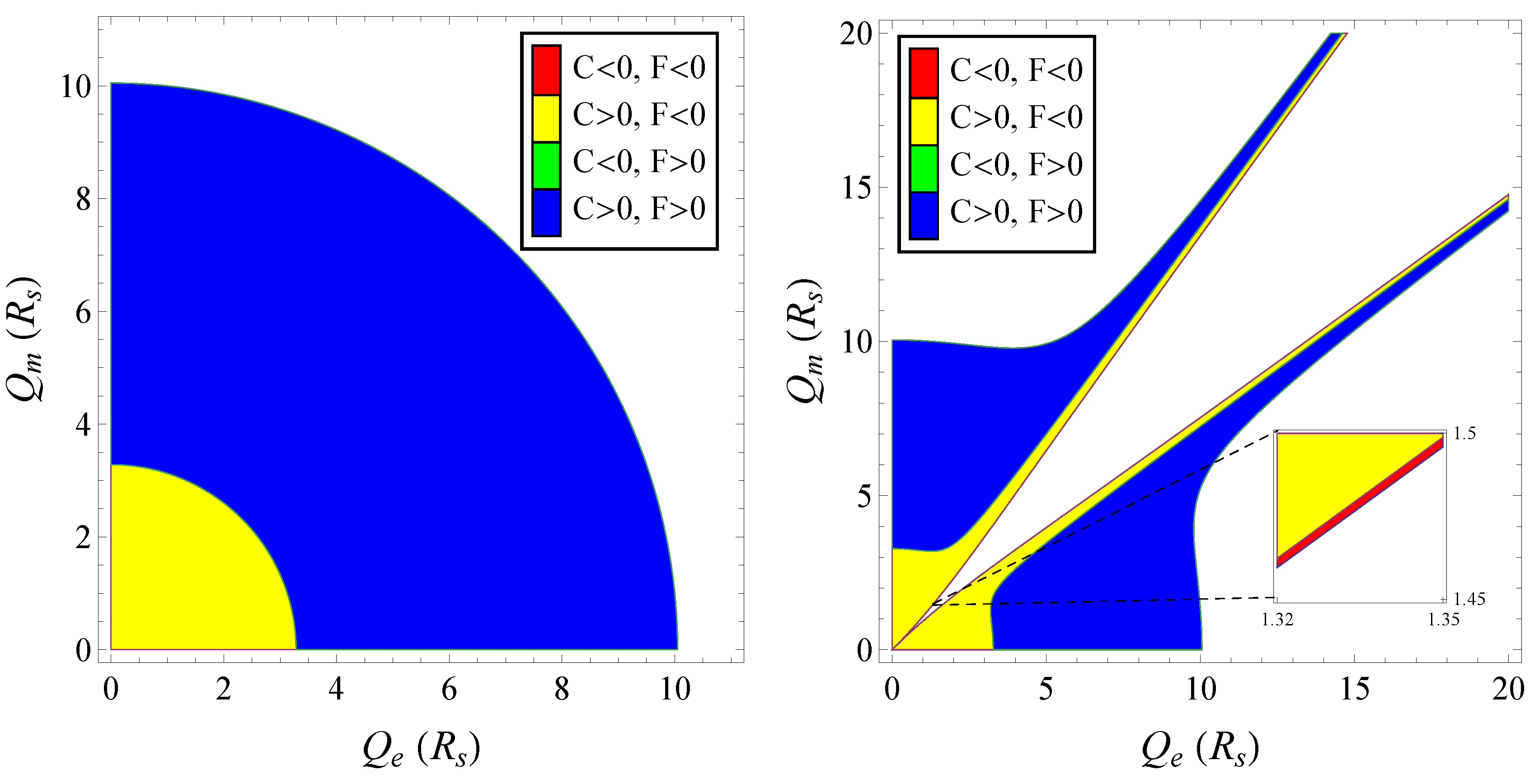
are stable. In the left panel of
Figure 1 we have represented the phase diagram of a RN BH solution in standard Electrodynamics, whereas in the right panel it is represented the phase diagram of a RN-like BH solution in the IE Model for negative
ε. From this figure, we can observe the IE Model presents new features, namely, that a new phase with both
C and
F negative arises in the IE Model. This phase is actually absent in standard Electrodynamics. There is also another phase that is not depicted in the figure, corresponding to negative heat capacity and positive free energy, but it appears in both models for lower values of Λ (and, particularly in flat space,
) [
23].
Figure 1.
(Left panel) Phase stability regions for a Reissner-Nordström (RN) black-hole (BH) solution with (being the Schwarzschild radius of a BH with a solar mass, , in Planck units ), and , in standard Electrodynamics; (Right panel) Phase stability regions for a RN-like BH solution with , and in the Inverse Electrodynamics (IE) Model. We can observe that a new phase exists, with both F and C negative, which does not appear in standard Electrodynamics.
3.2. Classification of RN-Like BH Solutions in Terms of the Number of Phase Transitions
Additionally, it is possible to provide a classification in terms of the number of phase transitions that the BH solutions host. In other words, the number of divergences of the heat capacity Equation (
20) as a function of the horizon radius [
16,
17,
36,
37,
38]. Thus, in the IE Model the following nomenclature can be used [
23]:
fast BHs, with no phase transitions, corresponding to
Λ;
slow BHs, with two phase transitions, corresponding to
Λ; and
inverse BHs, with a unique phase transition, corresponding to
. The latter class of BH solutions does not appear in standard Electrodynamics, but it also arises in other non-linear theories, as for instance in the Born-Infeld model [
11]. In
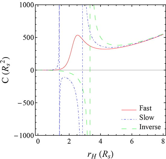
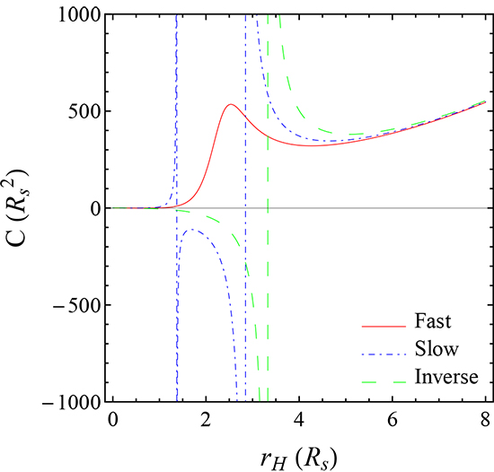
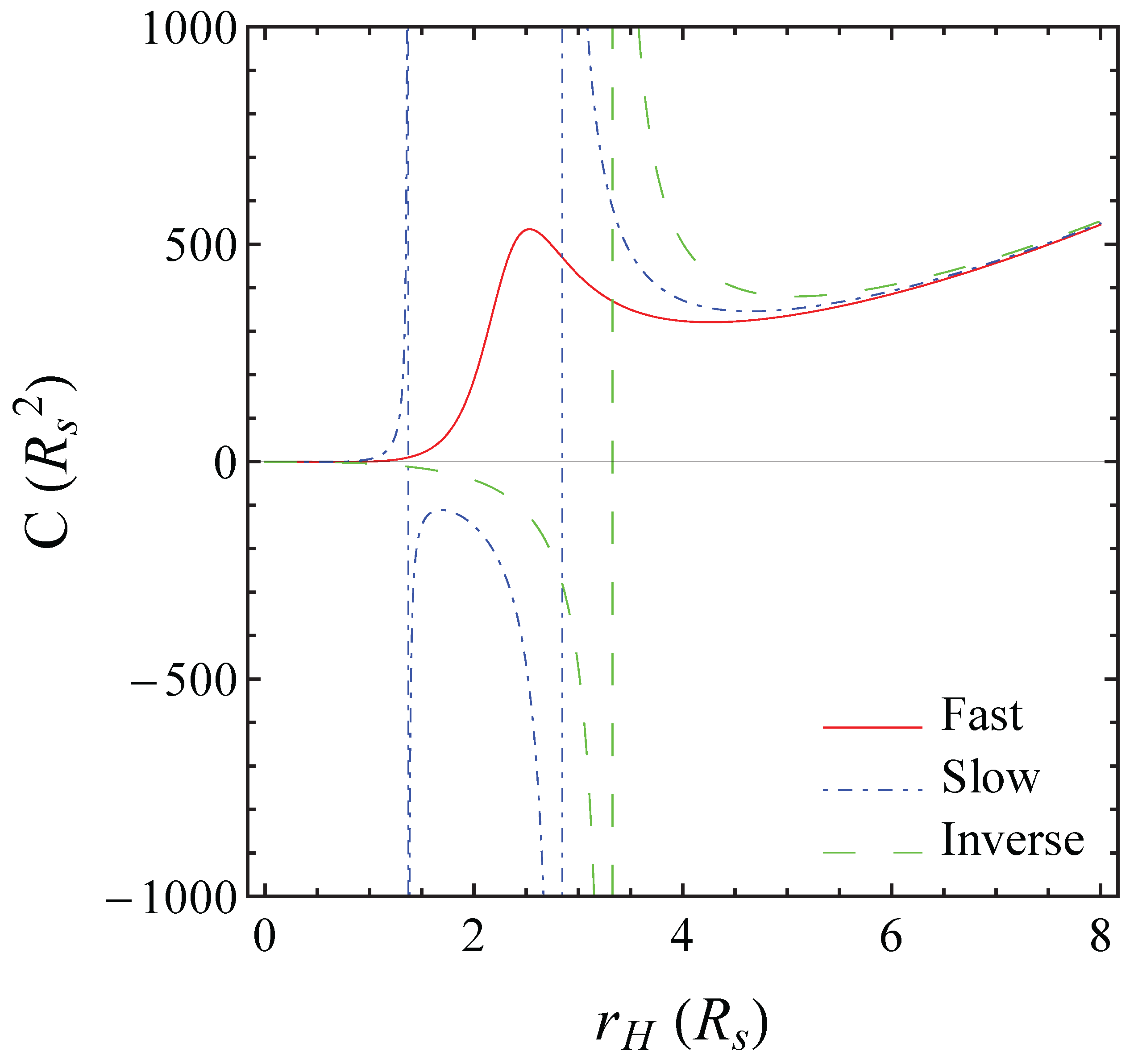
Figure 2 we have provided one example of each of these classes of BHs.
Figure 2.
Heat capacity as function of the horizon radius for different classes of RN-like BH solutions. In the IE Model we can distinguish between fast BHs, with no phase transitions; slow BHs, with two phase transitions; and inverse BHs, with a unique phase transition. The parameters used for each BH solution were: (1) Fast (red solid line), , , , ; (2) Slow (blue dot-dash line), , , , ; (3) Inverse (green dashed line), , , , .
4. Conclusions
In this paper we have studied the Inverse Electrodynamics Model: a non-linear Electrodynamics model that respects the parity, gauge and conformal invariances of standard Electrodynamics, and which, when coupled to General Relativity, also provides static and spherically symmetric (Reissner-Nordström-like) black-hole solutions.
Furthermore, using the Euclidean action method, we have performed a thermodynamic analysis of these Reissner-Nordström-like solutions, studying both the stability regions of the solutions and the number of phase transitions. First, we have observed that the Inverse Model supports a new stability region of black-hole solutions, with both the heat capacity and the free energy negative. This kind of solutions will be then less energetic than pure radiation and consequently they do not decay via tunneling. Moreover, since they have negative heat capacities, they will decrease their temperature under acquiring mass. Finally, we have also seen that in the Inverse Electrodynamics Model black holes with a sole phase transition exist, a non-existing feature in standard Electrodynamics. Hence, we conclude that although the gravitational solutions of both Electrodynamics models could be thought to be the same, the thermodynamics properties greatly differ. Further investigation and generalisation of this model are in progress.


