
Expanding Space, Quasars and St. Augustine’s Fireworks

1
Polytechnique, 91128 Palaiseau, France
2
Department of physics, Novosibirsk State University, Novosibirsk 630 090, Russia
3
Budker Institute of Nuclear Physics SB RAS and Novosibirsk State University, Novosibirsk 630 090, Russia
*
Author to whom correspondence should be addressed.
Universe 2015, 1(3), 307-356; https://doi.org/10.3390/universe1030307
Submission received: 5 May 2015
/
Revised: 29 August 2015
/
Accepted: 14 September 2015
/
Published: 1 October 2015
Abstract
:An attempt is made to explain time non-dilation allegedly observed in quasar light curves. The explanation is based on the assumption that quasar black holes are, in some sense, foreign for our Friedmann-Robertson-Walker universe and do not participate in the Hubble flow. Although at first sight such a weird explanation requires unreasonably fine-tuned Big Bang initial conditions, we find a natural justification for it using the Milne cosmological model as an inspiration.
Keywords:
quasar light curves; expanding space; Milne cosmological model; Hubble flow; St. Augustine’s objectsPACS classifications:
98.80.-k; 98.54.-h- You’d think capricious Hebe
- feeding the eagle of Zeus,
- had raised a thunder-foaming goblet,
- unable to restrain her mirth,
- and tipped it on the earth.
F.I.Tyutchev. A Spring Storm, 1828. Translated by F.Jude [1].
1. Introduction
“Quasar light curves do not show the effects of time dilation”—this result of the paper [2] seems incredible. The cosmological time dilation is a very basic phenomenon predicted by the Friedmann-Robertson-Walker (FRW) metric. How can quasars ignore this fundamental effect of relativistic cosmology?
Of course, extraordinary claims require extraordinary evidence. Until the puzzling results of [2] are firmly confirmed by independent observations, we cannot be certain that what is observed in [2] is a real observation of time non-dilation in quasar light curves and not a some unaccounted systematic error, for example, in data analysis.
Nevertheless, we will assume in this article that the results of [2] are correct and try to explain why quasars behave like strangers in our FRW world. Strangely enough, our main idea came from Fyodor Tyutchev’s poetry (see the epigraph). The image of capricious Hebe tipping a quasar-foaming goblet on our universe was a poetic metaphor guiding this investigation and what follows can be considered as an attempt of more or less scientific incarnation of this irresistible metaphor.
The paper is organized in five parts. In the first section we consider caveats of the standard picture of expanding space as a rather subjective notion. On the other hand, in contrast to expanding space, which can be considered as a kind of coordinate artifact, cosmological time dilation is argued to be an unavoidable, coordinate independent prediction for any internal time variability of any object participating in the Hubble flow. Therefore, if quasars really manage to escape bonds of time dilation, a natural inference will be that they somehow do not participate in the Hubble flow. This quasar mystery is accompanied with some others that are discussed in the second section.
The following section gives a detailed description of the Milne model. In the ideal case, the Milne universe is a part of the Minkowski space-time with the future light-cone of the Big Bang event as its impenetrable boundary. However, the density of the Milne fundamental observers, tending to infinity on this boundary, makes unrealistic the realization of the ideal Milne universe. This conclusion is further strengthened if we consider a quantum scalar field in the Milne universe: if the boundary is assumed to be impenetrable, the corresponding choice of the initial vacuum state is not an adiabatic but a conformal vacuum that leads to the pair production phenomenon indicating the presence of physically unrealistic infinite power sources on the Milne universe’s singular boundary.
In the forth section it is argued that in any realistic incarnation of the Milne universe it is expected that objects from “outside” can penetrate inside the Milne universe. Then we postulate that the existence of analogous objects in our universe is possible and we comment how these objects which do not participate in the Hubble flow due to their “otherworldly” origin, can offer an explanation of some quasar mysteries.
In the final section we provide concluding remarks and discuss how the result of this work can be related to other ideas described in the literature.
We have tried to make the paper as self-contained as possible by providing enough details of all calculations, and we hope that “the reader will not need to have his fingers at eleven places to follow an argument” [3].
2. Space Expansion and Enigma of Time Non-Dilation in Quasar Light Curves
Expansion of space is, probably, the most familiar concept in modern cosmology. However, this beguilingly simple idea harbors many dangers of misunderstanding and misuse even for professional physicists, “most scientists think they understand it, but few agree on what it really means” [4]. It is not surprising that the subtle notion of expanding space became a subject of continuing debates [5,6,7,8,9,10,11,12,13,14,15], largely triggered by a beautiful Scientific American article by Lineweaver and Davis [4].
We can identify at least two main reasons why it is dangerous and misleading to speak about expanding space without explicitly clarifying what is really meant by this combination of words.
First of all, as special relativity teaches us, space by itself does not constitute an objective reality—only space-time does. As eloquently expressed by Minkowski “Henceforth, space by itself and time by itself are doomed to fade away into mere shadows, and only a kind of union of the two will preserve an independent reality” [16]. It does not make sense, therefore, to speak about expanding space without clarifying what foliation of space-time we have in mind and why we have chosen this specific foliation.
In general relativity understanding is further complicated by the fact that coordinates loose their usual meaning as temporal and spatial labels of events. We can use any coordinate system in general relativity to describe a given physical phenomenon and we should be very careful to separate the real physical events from mere coordinate artifacts. Moreover, when we speak about temporal development in space of some physical process, we should specify what coordinate system was chosen and for what reason. Without doing so, “to some degree we mislead both our students and ourselves when we calculate, for instance, the mercury perihelion motion without explaining how our coordinate system is fixed in space, what defines it in such a way that it cannot be rotated, by a few seconds a year, to follow the perihelion’s apparent motion …Expressing our results in terms of the values of coordinates became a habit to such an extend, that we adhere to this habit also in general relativity, where values of coordinates are not meaningful per se” [17].
It is the symmetry of space-time, namely isotropy and homogeneity of space, which determines its preferred foliation. More precisely, the cosmological or Copernican principle states that we do not occupy a special place in the universe, which, at large, is very much the same everywhere at any given instance. Mathematically this means (see, for example, [18]) that the space-time can be foliated into spacelike slices and has a form , where every spacelike slice Σ is a maximally symmetric space (homogeneous and isotropic) and represents the cosmic time (a succession of instances of “now”). Geometrically the cosmic time is essentially the parameter that labels spacelike slices and each slice hypersurface is an orbit of the symmetry group of spatial homogeneity and isotropy [19].
The metric which corresponds to this preferred foliation is the celebrated Friedmann-Robertson- Walker metric (in units where ):
with , or corresponding to the close, flat or open universes respectively.
The expansion of space has a clear meaning in FRW coordinates: the scale factor depends on cosmic time. The particular form of this dependence is determined from Einstein equations. However, this fact does not mean much without connecting it to real physical observables: as was mentioned above, we should distinguish real physical effects from coordinate artifacts.
One coordinate artifact is the singularity (for positive k) of Equation (1) at and it can be removed by introducing a new radial coordinate ψ according to [20]:
where the generalized sine function is defined as follows [21,22]:
In new coordinates the metric takes the form [20]
How can we be sure that the time dependence of the scale factor cannot be similarly removed by a suitable change of coordinates? For example, let us consider the following cosmological model. The metric Equation (1) has two characteristic length scales both of which in general evolve in time: the spatial curvature radius and the Hubble length , where is the Hubble parameter that sets the time scale of the cosmic expansion. An attractive possibility is the perfect cosmological principle that the universe at large is not only homogeneous in space but also in time. Bondi’s derisive formulation [20] “Geography does not matter, and history does not matter either” expresses the perfect cosmological principle more eloquently. It is immediately obvious that for the non-dependence on time of the curvature radius and of the Hubble length, it is necessary to have and with some constant which can be absorbed into the exponential part and then eliminated by a time translation (by suitable redefinition of the origin of time scale). Thus, the metric takes the form:
This beautiful theory, based on the perfect cosmological principle, used to be a base for the steady state theory (see, for example, [23]) before the latter being killed by some ugly observational facts [24]. However, nowadays this de Sitter cosmology surprisingly resurrected as a possible description of reality as it may correspond to universe’s initial inflationary phase or its terminal state.
Let us introduce the new coordinates instead of through relations (see, for example, [10]):
In this so called static coordinates the metric Equation (5) becomes
The static coordinates determine another slicing (foliation) of the de Sitter space, which doesn’t show any sign of space expansion. What about other foliations?
Let us introduce the following fancy coordinatization of the de Sitter space:
This set of five coordinates is obviously not independent as the de Sitter space-time is four dimensional. From Equation (8) we easily find that
Therefore, these coordinates define a four-dimensional hypersurface in the five-dimensional space. The really remarkable fact about these coordinates is however that the de Sitter expanding metric Equation (5) on this hypersurface is induced by the five-dimensional Minkowski metric in the ambient space:
This can be easily checked by explicit calculations starting from relations Equation (8). But these coordinates are in fact based on the symmetry considerations [25].
Thus, the de Sitter universe can be considered as a highly symmetric four-dimensional hypersurface (a Minkowskian sphere) in circumambient five-dimensional Minkowski space-time. Each foliation, which endows this Minkowskian sphere with a sense of time, are on equal footing according to the spirit of relativity. However, the cosmological circumstances can dictate the preferred foliation. For example, the exponentially expanding universe Equation (5) corresponds to the sense of time of comoving observers for which the cosmic microwave background is isotropic and the universe itself is spatially flat. However, other foliations exist and can give closed or open universes [25,26]. Namely, if we define comoving FRW coordinates as:
the ambient Minkowski metric induces on the four-dimensional Minkowskian sphere the metric:
which corresponds to the close, cosmological constant dominated, FRW universe. While using the coordinatization
we get an open, cosmological constant dominated, FRW universe with the metric
As we see, the notion of expanding space is rather subjective. Only comoving observers (galaxies) would find it natural, and our insistence on using this notion reflects our belief that there is no other natural set of observers which would define a different preferred foliation for cosmology. Nevertheless, it seems that quasars dispute this common wisdom and do not find expanding space natural.
Cosmological redshift is usually associated with the expanding space. However, in contrast to the expanding space, redshift is a directly observable objective property of light signals emitted by distant sources.
Suppose two light signals are emitted at cosmological times and in a distant galaxy at the comoving coordinate ψ. We at will receive signals at cosmological times and . How are and related to each other? We can find this relation as follows [20].
Light propagates along null-geodesics or with along its world-line. Then, for radially propagating light-signals we have from Equation (4) and, therefore,
Hence, we obtain the cosmological time dilation relation
As its derivation indicates, it is an elementary and general consequence of general relativity and space-time geometry. Usually this time dilation relation is applied to redshifts: if represents the period (inverse frequency) of light-wave with the wavelength , then the redshift
The derivation of the cosmological time dilation relation Equation (16) is the most simple in the comoving coordinates where it can be interpreted as a result of the space expansion. But we can still use any other coordinates. Let us consider, for example, the de Sitter space-time in static coordinates where nothing expands or shrinks and rederive Equation (16).
For radial light propagation, we have from Equation (7) that
(R decreases when the light signal moves towards us from a distant galaxy. Hence the minus sign). We obtain then the following relations:
Assuming infinitesimal and , we can easily get from Equation (19)
The coordinate r of a comoving galaxy does not change with time; taking it into account, the second relation in Equation (6) indicates that
Using this expression and , we get from Equation (20)
But the coordinate time is not the time that clocks of the comoving observers actually measure. The latter according to Equation (5) is just the cosmic time , and the first equation in Equation (6) together with Equation (21) indicate the following relation between them
Therefore,
The fact that Equation (24) is the same relation as Equation (16) is not obvious, but can be shown as follows [10]. Along a null radial geodesic from to , we have according to Equation (5) and respectively
Which proves that Equation (16) and Equation (24) relations are equivalent. However, the physical interpretation of the cosmological time dilation in static coordinates is different. The relation following from Equation (7):
between the cosmic time t (the proper time of comoving observers) and the coordinate time T, where
can be interpreted [10] as resulting from both the gravitational redshift due to “potential” , and the kinematical effect (the Doppler shift) due to the Hubble recession velocity of the light-source.
As the discussion above shows, in contrast to the expanding space, which is a subjective notion depending upon the coordinate choice, the cosmological time dilation is an objective and very basic phenomenon with the important observable consequence that the rate of any time variation of the radiation emitted by a distant source with the cosmological redshift z should be proportional to (see Equation (16) and Equation (17)).
There is no way to escape this conclusion under the standard belief that all distant astrophysical objects participate in the Hubble flow. Therefore, it is not surprising that observations of distant type Ia supernova confirms this time dilation prediction [27] (it was suggested long ago to use supernova to detect the time dilation [28]).
However, a recent study of over 800 quasar light curves found no evidence of the expected effects of time dilation [2]. This is a very surprising result with no explanation within the conventional cosmological framework (note that some studies report the lack of time dilation signatures also in gamma-ray burst light curves [29,30]. See however [31,32]).
Some non-conventional explanations were proposed in [2], for example, the idea that the expected effects of the quasar time dilation are exactly compensated by an increase in the intrinsic timescale of quasar variability due to the growth of the quasar black holes, or that the observed variations are not intrinsic for quasars but are caused by microlensing events at much lower redshifts. Nonetheless, these explanations do not seem plausible.
We will try to argue in this note that this surprising result, if confirmed without any doubt, will imply a radical change of our cosmological perspective, namely that (at least some) quasars are related to the pre-Big-Bang objects, which we call St. Augustine’s objects for reasons explained later. These objects would define a preferred foliation different from the preferred foliation of the Hubble flow comoving observables and this new preferred foliation implies a pre-existing space-time predating the Big Bang.
Perhaps some comments are appropriate here. Application of the cosmological principle assumes that the cosmic time and the corresponding three dimensional space, defined as a set of simultaneous events according to this cosmic time, are well defined concepts in cosmology. It may seem that this is obvious and should be taken for granted. However, Gödel’s discovery [33] of cosmological space-time with closed timelike curves passing through every event made it clear that in general, the existence of global cosmic time is not at all guaranteed (the first example of space-time with closed timelike curves was in fact given by Lanczos [34] in 1923 and then rediscovered by van Stockum [35] in 1937). The existence of cosmic time requires a condition which is stronger than causality. Namely, a space-time admits a cosmic time if and only if it is stably causal [36]. Space-time is stably causal if closed timelike curves are not only absent but they do not appear even after a deformation of the space-time metric which slightly opens up the light cones all over the space-time [37,38,39].
Friedmann-Robertson-Walker metric is stably causal and therefore admits the cosmic time. However, it is the matter content of the universe (cosmic substratum) and motion pattern of this substratum which actually endow the cosmic time and Friedmann-Robertson-Walker metric with the real physical meaning via celebrated Weyl’s principle [40,41]. Weyl’s principle is an assumption about the nature of the Hubble flow and it states that world lines of the “fundamental particles” of the cosmic substratum (usually assumed to be galaxies or clusters of galaxies) form, after averaging over the peculiar motion, a space-time-filling family (congruence) of non-crossing geodesics converging towards the common past [41]. Friedmann-Robertson-Walker metric holds a privileged position as it is co-moving with the fundamental observers. The above mentioned congruence of world lines is unique in the FRW space-time and thus defines its preferred foliation into spatial hypersurfaces that are ordered in cosmic time.
Unlike the FRW space-time, in the de Sitter space-time there is no unique choice of congruence and that’s why the de Sitter space-time can be considered either as a static or as an expanding universe [41].
When we speak about St. Augustine’s objects it is in fact assumed that the FRW space-time is only a part of a bigger entity (imagine, for example, an embedding of a spatially flat FRW space-time into the five-dimensional Minkowski space considered at the end of the paper) and that motion pattern of the cosmic substratum in other parts of this encompassing space are quite different from the Weyl congruence defining the Hubble flow.
3. Other Quasar Mysteries
Quasars (Quasi-Stellar Objects) are fascinating objects discovered half a century ago [42,43]. Shortly after their discovery, Zel’dovich [44] and Salpeter [45] independently suggested accretion on a black hole as an energy source of quasars. This hypothesis became universally accepted after the publication of Lynden-Bell [46] showing that the main properties of quasars could indeed be understood in terms of release of gravitational binding energy of matter accreting onto a supermassive black hole. Nevertheless, quasars largely remain the most mysterious and enigmatic objects in the Universe and even the most basic and major questions about them are far from being settled [47,48,49]. Let us briefly outline some problems in quasar research with no definite answers [49].
3.1. The Origin of Supermassive Black Holes
If we adopt the standard view that the observed quasar redshifts are of cosmological origin, when the unavoidable consequence is that the quasars are immensely bright: brighter than thousands of the brightest galaxies at low redshifts. At that strong variability of quasars in short time scales indicates that the majority of this immense energy is emitted from a tiny region not exceeding the Solar System in size. Supermassive black holes are indeed the only powerhouses that can be imagined to meet such extreme energy and size requirements.
A simple argument why the central black hole in quasars should be supermassive goes as follows [50,51,52]. Let us assume a steady accretion so that the inward gravitational force acting on a small element of accreting gas of density ρ in the gravitational potential Φ of the black hole is balanced everywhere by the radiation pressure force on this gas element. If the gas is fully ionized hydrogen then radiation pressure force acts mainly on free electrons through Thomson scattering (for protons the scattering cross section is smaller by the factor ). However, due to Coulomb attraction, the electrons drag the protons with them so that the charge separation does not occur). The Thomson cross section gives the effective area for an electron to absorb radiation when it is illuminated. Therefore, if the radiation energy flux is , each electron absorbs momentum at a rate . The radiation pressure force equals the rate at which the volume element absorbs momentum. In this volume element we have protons and hence, the same amount of electrons, as the gas is assumed to be fully ionized. Therefore,
Then the condition of hydrostatic equilibrium, , gives the equation
Using this relation, the Gauss’s theorem and the Poisson equation , G being the Newton constant, we can calculate the total luminosity as a surface integral over some closed surface S around the quasar:
Therefore, finally,
where M is the quasar mass. This so called Eddington luminosity is an estimate of the maximal luminosity a quasar of mass M can have if it is powered by a steady accretion. Substituting and other physical constants, Equation (30) can be rewritten as follows [50]
where is the solar mass. Typical quasar luminosity is [52]. Then Equation (31) indicates that a central mass of the order of is required.
Various methods were developed in past decades to estimate quasar masses from observations [53] and the results confirm the above conclusion that quasars are supermassive. Moreover, the results indicate [53] that quasars with masses were probably already present at when the universe was less than 1 Gyr old. This raises a potential problem: how these supermassive black holes have had grown up given the limited time they had?
If the accretion rate is μ, then the associated luminosity can be written as , with ϵ representing the radiative efficiency that equals the fraction of the accreted rest energy converted into radiation. The growth rate of the black hole under such accretion is . Therefore, from these two relations, using the Eddington luminosity Equation (30), we get
where
is the so called Salpeter time. Equation (32) indicates that under the steady Eddington accretion the black hole mass grows exponentially with time:
where is the mass of the black hole seed. What can we say about the radiative efficiency ϵ? To estimate ϵ, we can use a Newtonian argument. In fact not quite Newtonian, because the pure Newtonian estimate, assuming that the accretion disk extends up to the Schwarzschild radius, is a factor of two higher than the more appropriate general relativistic result. However, it was shown be Paczyńsky and Wiita that the following simple pseudo-Newtonian potential
reproduces the correct general relativistic results surprisingly accurately as far as the black hole accretion flaw is concerned [54,55]. Here, is the Schwarzschild radius of the black hole.
For a test body of mass m moving on a circular orbit of radius r in the potential Equation (35), we find for its velocity
and for its total energy
As we see, only for the bound circular orbits are possible. But not all of them are stable. The stability condition is the following:
where U is the effective potential corresponding to the orbital momentum l. The orbital radius r is determined from the condition
This enables us to exclude l and rewrite the stability condition in the form
Therefore, only circular orbits with are stable and hence, the steady accretion disk ends at . The binding energy at this innermost stable orbit is, according to Equation (36),
When the particle of mass m migrates from the outskirts of the accretion disk at , where its binding energy , to the inner edge of the accretion disk, this energy is released as heat and eventually radiation. Therefore, the radiative efficiency of such a Schwarzschild black hole engine is . More correct treatment of general relativistic effects gives [56]. Rotating black holes can lead to even higher radiative efficiencies: up to about in realistic case [56]. For comparison, nuclear burning of hydrogen to helium in stars has the efficiency of only .
Usually, in quasar research one assumes a canonical radiative efficiency of [53]. For at and Gyr that corresponds to when the first stars were formed, we get from Equation (34) that the black hole seeds of mass is needed. This seems somewhat high as it is expected that the black hole remnants from the first generation stars had typical values less than tens of solar masses [53].
Although this is not considered as an immediate problem, because we could imagine ways how to produce such massive black hole seeds (for example, direct collapse of primordial gas clouds [53]), but it will be fair to say that we do not completely understand the origin of supermassive black holes at present. Even if we would have a sufficiently massive black hole seed, it is not clear how a steady accretion at Eddington rates can be maintained for such a long period of time. The accreting gas has to lose about of its angular momentum to migrate from the host galaxy to the vicinity of the black hole [57]. During this time, various processes can intervene to make the accretion not continuous. For example, star formation which inevitably occur in the accretion disks on large scales, can reduce the amount of gas which can be directly accreted onto the black hole [50,57]. In fact, our present day arguments about how quasars ignite and produce their stupendous energies are of the kind of hand-waving lacking necessary details [58] and so we still do not have good predictive physical models [48].
3.2. Evolution of Quasars and Age Problems
Another mysterious thing about quasars which is poorly understood is the evolution of quasar luminosity over redshifts: quasars at high redshifts are far more luminous than quasars at low redshifts [49]. But, strangely, quasar spectra show little evidence, if any, of this evolution: quasar spectral features at low and high redshifts are very similar [49]. It seems that quasars were already mature at and the physical properties of their accretion disks have not changed since then despite strong evolution of their luminosities.
Not only quasars at high redshifts seem to be mature but their surroundings too. It is assumed that it requires many generations of supernovae to produce sizable amount of metals. So, the natural expectation is that the accreting material for high redshift quasars should be metal-free. Observations, on the contrary, indicate that metallicities are even higher than the solar metallicity [49]. Recent discovery of galaxy with significant metallicity and very high star formation rate [59] also indicates more rapid chemical evolution in the early universe than it is usually assumed.
Some quasars were found [60] at without any detectable infrared emission from the hot dust which is expected in the standard accretion disk model and is indeed universally present at low redshifts. This may be a sign of the long evolution of quasars absent in the ultraviolet, optical and X-ray bands of their spectra. However, the rarity of such dust-free quasars indicate a very rapid mass accretion and dust formation at their alleged early evolutionary stages [60].
Another question is what ignites a quasar. It is usually assumed that the major merger events of gas-rich galaxies trigger the accretion on the central black hole and ignite a quasar. However about half of host galaxies have undistorted disks and show no signs of distortions induced by merger [49].
Besides the problem of explaining the appearance at a surprisingly early times after the Big Bang of chemically mature galaxies hosting a supermassive black holes, there is still another age problem related to quasars. Namely, a quasar was discovered at whose age is 2–3 Gyr, while according to the standard cosmological model the Universe was only 1.63 Gyr old at this redshift [61]. Therefore, this quasar appears to be older than the Universe—an obvious paradox requiring explanation.
While the so called α-process elements (O, , , , S) are mainly produced in type II supernovae, the so called iron-peak elements (V, , , , , ) are produced in type Ia supernovae [62,63]. The corresponding characteristic time scales are vastly different which enables to estimate the age of astrophysical objects by measuring their abundance ratios.
Type II supernovae are explosions of massive stars induced by the collapse of their inert iron-nickel cores when the core exceeds the Chandrasekhar limit of about 1.4 solar masses and the electron degeneracy pressure in the core is no longer sufficient to maintain the equilibrium against gravity. The lifetime of such massive stars () is quite small, about years.
Type Ia supernovae are thermonuclear explosions of accreting carbon-oxygen white dwarfs in close binaries. The lifetime of such binaries, estimated from the chemical evolution of our galaxy, is about 1 Gyr [63], although a lifetime distribution can span within a wide range of 0.1–20 Gyr [64].
As it was already mentioned, this difference in timescales gives us a specific “clock” to measure the age of astrophysical objects. In the case of the quasar APM 08279+5255 at , using the measured abundance ratio and a detailed chemodynamical model, it was estimated [65] that the age of this quasar is Gyr.
The age of the Universe at this redshift can be obtained in the following way. From Equation (17), with the identifications , , where is the present age, we get
On the other hand, the Hubble parameter is given by the Friedmann equation which for the flat Universe () takes the form (see, for example, [20]):
, and being the energy densities of matter, radiation and vacuum, respectively. The vacuum energy density (the so called dark energy) does not depend on the scale factor. The matter energy density scales as and the radiation energy density as (because in this case not only the photon number density decreases as upon space expansion, but also each photon experiences a redshift and its energy decreases as ). Therefore, we get from Equation (38),
where
are the present fractional energy densities of matter and radiation given in terms of the critical density
and we have taken into account that for the flat Universe .
Equation (39) gives the Hubble parameter as a function of redshift. Therefore, we can separate variables in Equation (37) and get the following integral (note that at the Big Bang, t = 0, the scale factor is zero and hence the redshift is infinity) [65]:
This is an elliptic integral. However, if we ignore the radiation energy density, which is very small at present epoch () and becomes important only at very high redshifts hence contributing little in the integral Equation (40), then the integral can be calculated in terms of elementary functions by a sequence of substitutions [66]
and we finally get [66,67]
For , and , Equation (41) gives Gyr and we have the above mentioned age problem .
3.3. Correlation of Quasars with Galaxies of Lower Redshifts
A long standing controversy is an alleged association of high-redshift quasars with low-redshift galaxies [49,68,69,70]. Some quasars are surprisingly close, only a few arcseconds away, to the galaxies with widely different redshift. In some amazing cases filaments apparently connecting the pairs of objects with different redshifts have been observed. Maybe one of the most impressive cases is the Seyfert galaxy NGC 7603 [71,72]. Seyfert galaxies, less energetic cousins of quasars, are spiral or irregular galaxies containing an extremely bright quasar-like nucleus. The redshift of NGC 7603 is . There is another smaller galaxy, NGC 7603B, with nearby and the two are apparently connected by a narrow luminous filament, NGC 7603B lying at the end of the filament. The redshift of the filament itself is (the same as for NGC 7603 within the measurement errors which are of the order of [71]). There are two more galaxies lying exactly on the filament: one with the redshift positioned near NGC 7603B, and the another one with positioned near NGC 7603 [71,72] (see Figure 1a in [71]).
Mainstream cosmologists simply ignore this kind of evidence supporting association of objects with different redshifts considering all these cases as a just random projections of background objects like constellations. They might be right in some cases but the statistics of anomalies seems to be too high and indicates that we do not completely understand these phenomena [49].
3.4. Apparent Superluminal Motion
The last conundrum related to quasars which we will discuss in this section is the problem of apparent superluminal motion [49,69,73,74]. In fact this phenomenon was predicted [75] before it was discovered following the development of Very Large Base Interferometry (VLBI) that allowed a very accurate mapping of the radio sources morphologies. It was found that in many radio galaxies and quasars there are several compact sources of radio emission that appear to move apart superluminaly in successive VLBI images [76].
Canonical explanation of this apparent superluminal motion (see, for example, [52]) is ingenious but simple enough to be used as an undergraduate problem for the first year physics students [77]. The standard derivation, however, is valid only for nearby sources as it ignores cosmological space expansion, and this fact is not sufficiently stressed in existing literature [78]. Therefore, to avoid a confusion, we provide, following [78], a derivation valid for all redshifts.
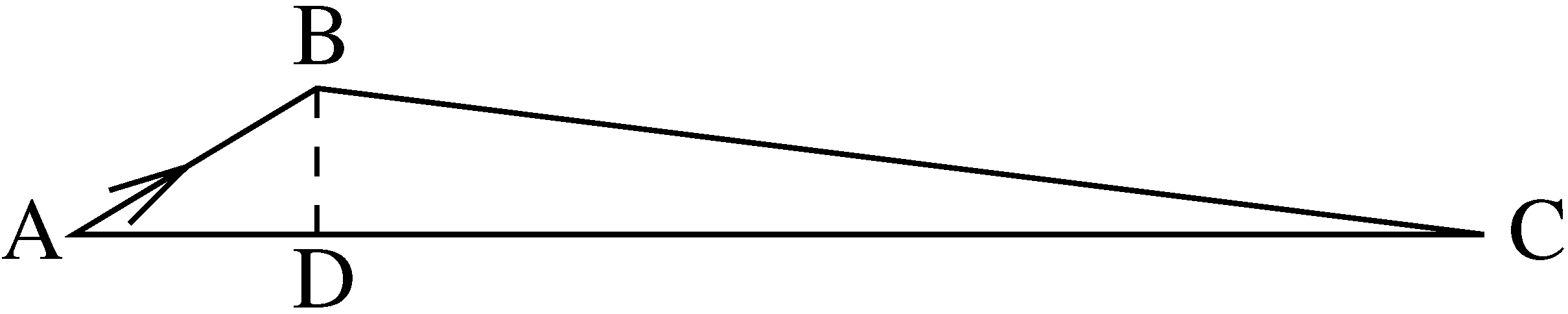
Suppose two radio emitting blobs coincide at a point A (see Figure 1) at cosmic time . The observer at a point C notices this coincidence at a later time because of the finite speed of light. One blob remains stationary while the other moves at a relativistic speed V towards the observer under a small angle to the line-of-sight of the observer. After infinitesimal time , the moving blob will reach the point B. The observer notices this event at time with some . As was already explained, in FRW universe the emission and reception times along radial null-geodesics are related as follows (in units where , so below we will use V and interchangeably)
where ψ is the co-moving radial coordinate of the point A, —of the point B and it is assumed that the observer is at the origin . From Equation (42) we have
On the other hand, the point B has, at the first order in , the same radial coordinate as the point D. Therefore,
Figure 1.
Relativistic beaming model of apparent superluminal motion

Therefore, the observed apparent transverse velocity of the moving blob with respect to the stationary one is [78]
The quantity which is actually measured on Earth is the observed angular proper motion of the moving blob on the sky per time unit and to transform it into the apparent transverse velocity we need to know the so called angular diameter distance . It is defined in such a way [20] that for a small solid angle the corresponding cross-sectional area at a distance is
On the other hand, for the FRW metric Equation (4), the total area of a sphere at cosmic time is and this area corresponds to the solid angle . Therefore,
From Equation (46) and Equation (47), we get . In particular, for the spatially flat universe,
To express Equation (48) in terms of observed quantities, we note again that for radial null-geodesics and therefore, by using Equation (17) and Equation (39), we get [78]
As we see, the apparent transverse velocity can be calculated from the observed quantities as follows
To concentrate on the intrinsic parameters of the source, it is a common practice to eliminate the redshift dependence of the apparent transverse velocity by considering (we have recovered the light velocity c for a moment)
Rather misleadingly, is widely called “apparent velocity” despite the fact that it is the apparent velocity only for a co-moving observer near the source [78]. The true apparent velocity for a terrestrial observer at a cosmological distance from the source is , as our derivation above indicates, and it is suppressed by a factor [78].
As a function of the angle θ, has a maximum when , where . As we see, can be arbitrarily large and at first sight relativistic beaming model gives a natural solution of the apparent superluminal motion problem. However, matters are not as simple as they seem.
We need , if we want . But then and is very small. If quasar jets are isotropically distributed in space, then the probability of observing an approaching jet with is (assuming that the quasar jets are double-sided and symmetrical) . This quite small probability indicates that the observation by chance of an apparent superluminal motion in quasars should be relatively rare phenomenon. It was clear from the beginning that real observations do not confirm this conclusion [79]. In fact apparent superluminal motion is common and ubiquitous in quasars [69,80]. For example, the MOJAVE (MOnitoring of Jets in AGN with VLBA Experiments) survey contains 101 quasars with 354 observed radio components, 95% of which move with apparent superluminal velocities with respect to the core. The maximum observed velocity equals to and about 45% of radio emitting blobs have velocities larger than [80].
A close inspection of the formula (50) indicates that it requires roughly to obtain . Then randomly, using the above mentioned probability , one would expect only blobs, out of 354, to have . In reality the observed number is 158—a totally improbable event by chance [80].
At this point, the relativistic beaming model is clearly in trouble. Fortunately for the standard paradigm, the Doppler boosting which is intrinsically related to the relativistic beaming comes at rescue. In particular, the observed flux density, , from an emitting blob which moves with a relativistic velocity towards observer making an angle θ with the line of sight is enhanced compared to the intrinsic flux from the blob at rest, , according to the formula [79,81]
where α is the spectral index of the radiating source (in other words, it is assumed that ). This relation follows from the relativistic invariance of and the Doppler blue-shift formula for the frequency [82]. Here is the specific intensity related to the flux density as follows [83]. Indeed, since , we have
To prove that is indeed relativistic invariant, we first show, following [83] (see also [84]), that a phase space volume element is Lorentz invariant. Let a group of particles occupy an infinitesimal volume around some radius-vector and have a slight spread of momenta around a mean momentum in some inertial reference frame S. In the frame , comoving with the particles, the mean momentum equals to zero and all particles have the same energy to the first order because the infinitesimally small momenta of individual particles contribute quadratically to their energy and therefore this contribution vanishes to the first order. Let us imagine some particle from the group with a momentum in the frame . Then in the frame S we have
and therefore the momentum spreads in the frames S and are related as follows
On the other hand, due to Lorentz contraction,
There is one subtlety here which sometimes can lead to confusion (see, for example, [85,86]). We need particles to occupy a given volume element simultaneously. But simultaneity is relative: if a group of particles are all inside a volume element at time t in reference frame S, in the comoving frame they are inside the corresponding volume element at different times and according to the Lorentz transformation the spread of these times around the mean time is . In the frame the particles are not in general at rest but move (in the x-direction) with infinitesimal velocities of the order of . Therefore, to bring all particles at the time instant will require a shift of their x-coordinates of the order of
Analogously, the required shifts in the y and z directions are
Fortunately, for finite m and γ, these quantities are of the second order and hence, can safely be ignored. Let us stress, however, that for this argument to be valid it is essential for to be the instantaneous comoving frame because only in this frame particle velocities are infinitesimal. If is not the comoving frame, we can no longer in general ignore the effects of desynchronization, and if we do, we get an erroneous conclusion, as in [85], that the phase space volume element is not Lorentz invariant.
Of course this reasoning is strictly valid only for particles of finite mass. However, the final result Equation (56) has no reference altogether to the particle mass and it is reasonable to propose that it should be true also in the limiting case of photons. Note, however, that Equation (54) and Equation (55) indicate that the limit is rather subtle. More formal and rigorous derivations of Equation (56) for photons can be found in [87,88].
Now let us consider an energy content of a phase space volume element occupied by monochromatic photons of frequency ν. It can be calculated in two different ways. First, from the definition of specific intensity, we have , where is the cross-sectional area of in the direction perpendicular to the photons mean momentum. On the other hand,
where we have used the relation and is the photon distribution function which is Lorentz-invariant because both and are Lorentz-invariant. Comparing these two expressions for , we see that [88]
This completes the proof that is Lorentz-invariant.
According to Equation (51), relativistic beaming has a very strong effect on the observed luminosity. For , and , the enhancement is about two orders of magnitude (this is true for a simple ballistic model of one radiating approaching blob for which Equation (51) applies. In the case of more realistic jet geometries the enhancement factor may be smaller [89]). This Doppler boosting effect allows to explain the above mentioned huge discrepancy in the statistical properties of observed superluminal sources as a kind of the Malmquist bias [80]. Simply, due to the Doppler boosting, it is natural to expect that flux-limited surveys of radio emitting sources will indeed preferentially pick up brighter sources that are ejecting material with small θ. However, this argument assumes that the main part of the observed flux, even the one that comes from the core, originates from relativistic jets, and not everybody is ready to except this assumption [90].
To conclude this section, at present we have no compelling reason to reject the standard cosmological concepts about quasars. However, it seems that there is a growing number of alleged observational facts which are difficult to reconcile with the standard paradigm. It is not a good strategy to simply ignore these facts, in our opinion. It would be much better to remember the nineteenth century humorist Josh Billings’ aphorism “It ain’t ignorance causes so much trouble; it’s folks knowing so much that ain’t so” [91] and keep eyes wide open to new insights.
4. The Milne Model
Let us consider a FRW universe with vanishing total energy density ρ and vanishing cosmological constant Λ. The Friedmann equation [20]
then gives (for not static universe) and . By rescaling the radial coordinate and time, we may assume that the units are such that the curvature constant is together with . Therefore, in this case the scale factor linearly grows with time. The possible integration constant can always be eliminated by a suitable change of the time origin. The metric Equation (4) takes the form
Such a space-time is called the Milne universe. It was Milne who realized that such a model must have an alternative, special relativistic description because it has the gravity “turned off” (vanishing energy density) and no cosmological constant [92,93,94,95]. Indeed, if we introduce new coordinates
the metric Equation (57) takes the form
which is just the Minkowski line element in spherical coordinates. Let us note that the Milne coordinates t and ψ cover only a part of the Minkowski space-time. Indeed, equations Equation (58) indicate that (because the cosmic time , corresponding to the Big Bang) and . Therefore, the Milne universe corresponds to the future light cone of the Big Bang event. To cover the past light cone, we can redefine the Milne coordinates , in such a way that
This leads to the same metric Equation (57) with a singularity at . For the expanding Milne universe Equation (58), the singularity corresponds to the Big Bang, and for the contracting Milne universe (with as a cosmic time), the singularity corresponds to the Big Crunch.
Equation (58) give , which for constant ψ represents a world-line of an observer uniformly moving radially with rapidity ψ. This clarifies the physical meaning of the Rindler coordinate ψ and suggests the following interesting interpretation of the Milne universe [96], originally due to Milne [92,93,94,95].
In the Minkowski space there is a point-like explosive event, the Big Bang, resulting in infinitely many debris of point particles (fundamental observers) shot out at all speeds up to the speed of light in all directions. It is possible to arrange a special kind of velocity distribution of fundamental observers for which the cosmological principle will remain true: all fundamental observers will see the identical velocity distributions. Indeed, let us show that this is possible [93]. Let be such a distribution. Because of the assumed isotropy of space, this distribution can depend only on the magnitude u of the velocity , not on its direction. The distribution function does not depend on time because after the Big Bang no new fundamental particles are created or destroyed and each of them moves with a constant velocity. The cosmological principle demands
where (according to our conventions, the light velocity )
is given by the relativistic velocity addition formula (see, for example, [97]). The Jacobian of this transformation is (to avoid involved calculations by hand, REDUCE Computer Algebra System [98] can be used to get this result)
where at the last step we have used the so called gamma identity [99,100]
Therefore, Equation (60) takes the form
and we see that (we have restored the light velocity c in the last formula for a moment)
with some positive constant B. This velocity distribution function has several remarkable properties [93]. The total number of particles is infinite and the velocity-centroid (the mean velocity) cannot be defined. The density of particles (in velocity-space) increases and tends to infinity as the velocity u approaches the light velocity. Each fundamental observer can be regarded as the stationary center of an expanding ball which looks one and the same for every choice of the fundamental observer. Not every explosion readily produces such kind of distribution. In fact, “it must have been an incredibly delicately tuned Big Bang to achieve this!” [96].
The Milne distribution Equation (62) is not of statistical but of hydrodynamic nature: the velocity of every fundamental particle at time T is uniquely determined by its position through the Hubble-like law
This fact allows to rewrite Equation (62) as a spatiotemporal distribution
with the particle density function
The density tends to infinity at the unattainable boundary of the expanding ball which moves away at the light velocity.
The density Equation (63) is inhomogeneous and therefore the Copernican principle is not evident in the Minkowski coordinates R and T. Of course, indirectly it is implemented through the equivalence of fundamental observers (cosmological principle). However, for the Milne universe there exists a natural foliation of space-time under which the spatial distribution of matter becomes homogeneous and thus the Copernican principle becomes obvious.
The symmetry group of special relativity (Minkowski space-time) is the ten parameter Poincaré group of inhomogeneous (including space-time translations) Lorentz transformations. The symmetry group of the Milne universe is a six parameter subgroup of the Poincaré group of homogeneous Lorentz transformations which leave invariant a special event—the Big Bang. As a result, there is a preferred class of inertial observers, namely those whose world-lines pass through the Big Bang event. The Milne universe is a description of the Minkowski space-time from the point of view of members of this preferred class [101]. The invariant proper time after the Big Bang
measured by the clocks of this fundamental observers, can be used for a natural definition of simultaneity in the Milne universe, alternative to the usual Einsteinian simultaneity (interestingly, Einstein’s definition of simultaneity by means of the light signal exchanges coincides, in principle, with the St. Augustine’s criterion of simultaneity given by him 1500 years earlier [102]).
This cosmic time t leads to the slicing (of a part) of the Minkowski space-time into space-like hypersurfaces Equation (64) (two-sheeted hyperboloids ) which Milne calls the public space to distinguish it from the private space of fundamental observers defined through the slicing, T being the usual Minkowski time. Note that immediately after the Big Bang (for every ) the public space is infinite, while the private space for every is a finite sphere of radius , increasing in size with light velocity as T goes on. Thus, the Milne model provides an excellent demonstration of a seemingly paradoxical situation that a point-like Big Bang can give birth to a universe with infinite spatial extension [96,103]. Interestingly, the Milne foliation of Minkowski space-time is exactly the foliation which leads to the Dirac’s point-form of relativistic dynamics [104,105].
Let be the density of particles in public space so that the number of particles in the volume element at cosmic time t is . For the metric Equation (57), the spatial components of the metric tensor are
Therefore, the square root of the absolute value of the determinant of the metric tensor equals to and
On the other hand, let us calculate the same number of particles in the private space. For fixed cosmic time t, the radial coordinates lay in-between and for the selected bunch of particles in the private space, where . But, according to Equation (58), this particles have different Minkowski time coordinates . Namely, the particles with the radial coordinate have the Milne coordinate and hence the T-time coordinate with . However, in private space the fundamental particles move radially outward with velocity . Therefore, at time T the bunch of particles have a reduced radial spread
and hence occupy volume element in the private space. The corresponding number of particles is
From Equation (65) and Equation (66), we get
where the last step follows from equations Equation (58), Equation (63) and Equation (64). As we see, the density depends only on cosmic time t and not on the position in the public space—the distribution of fundamental particles in the public space is not only isotropic but also homogeneous and the Copernican principle becomes explicit.
In more formal way, the same result can be obtained as follows [101]. The density-flow four-vector
where the density n is given by Equation (63), transforms under the change of coordinates
as follows
Differentiating , we get
which gives
Other portion of the partial derivatives can be obtained by differentiating . The results are
and correspondingly we get from Equation (69) .
Analogously, differentiating , we get
while differentiating , we get
Substituting these partial derivatives in Equation (69), we find that and . Therefore, in the Milne universe the density-flow four-vector has the form
We see that matter (fundamental particles) is at rest and uniformly distributed in the Milne Universe. As was already mentioned, the Milne distribution Equation (62) does not allow to determine the mean velocity of the whole system of fundamental particles and therefore the global standard of rest. However, using the mean motion of matter in the limited portion of space-time, we can define a local standard of rest in the neighborhood of a given point by defining rest and velocity relative to this mean motion. Introduction of the cosmic time and public space (co-moving coordinates) is just a realization of this strategy [101].
In the following, for simplicity, we will use a two-dimensional space-time to illustrate our arguments. The two-dimensional Milne metric has the form ()
How can imaginary intelligent observers in the Milne universe discover that their space-time is just a part of the more vast Minkowski space-time? The coordinate transformation Equation (58) is not simple enough to be trivially guessed. Instead we can envisage the following line of thoughts (adapted from [105]).
Null geodesics (light rays) can be used to construct a natural coordinate grid in the Milne universe. Coordinates with respect to this grid (null coordinates) are expected to convey and reveal the intrinsic geometry of the Milne space-time. According to Equation (72), null geodesics are determined by the condition
Integrating, we get that along null geodesics
where is an integration constant such that is dimensionless. Accordingly, we introduce null coordinates
The form of Equation (74) suggests to make further transformation
which brings the metric into the very simple form
Equation (75) indicate that the Milne space-time corresponds to the coordinate ranges and . However the metric Equation (76) is no longer singular and we can extend our space-time by allowing the whole ranges and . The identification
puts the metric in the canonical Minkowskian form and thus shows that our extended space-time is just the Minkowski space-time. The coordinate transformation, inverse to Equation (77), is
which implies the following relations between the Minkowski coordinates and the Milne coordinates (compare with Equation (58))
If we choose instead , we get the contacting Milne universe with
which correspond to the patch of the Minkowski space-time. What about and patches of the extended space-time? Let us take
Substituting into Equation (76), we get
Therefore, α is timelike and β is spacelike. Thus, we identify which brings the metric into the form
Such a metric is known as Rindler metric [20]. According to Equation (78), the Minkowski coordinates and Rindler coordinates are related as follows
It is clear from Equation (81) that we must have . Therefore the Rindler space-time corresponds to the portion of the Minkowski space-time (right Rindler wedge). The choice leads to the left Rindler wedge with the same metric Equation (82) but with
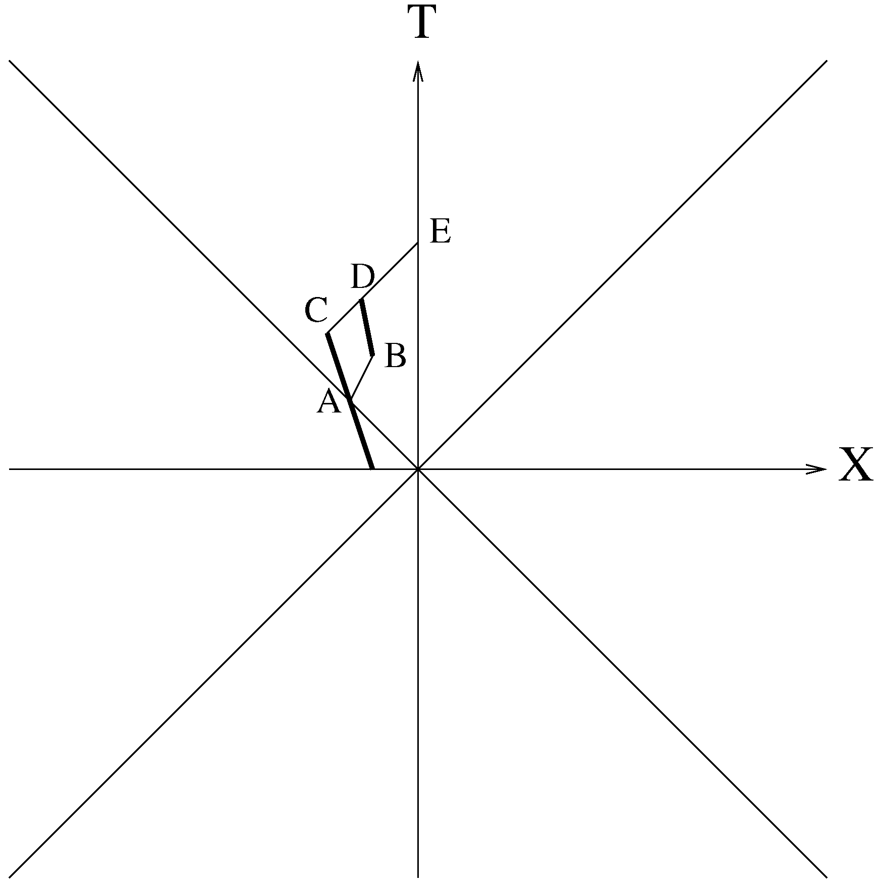
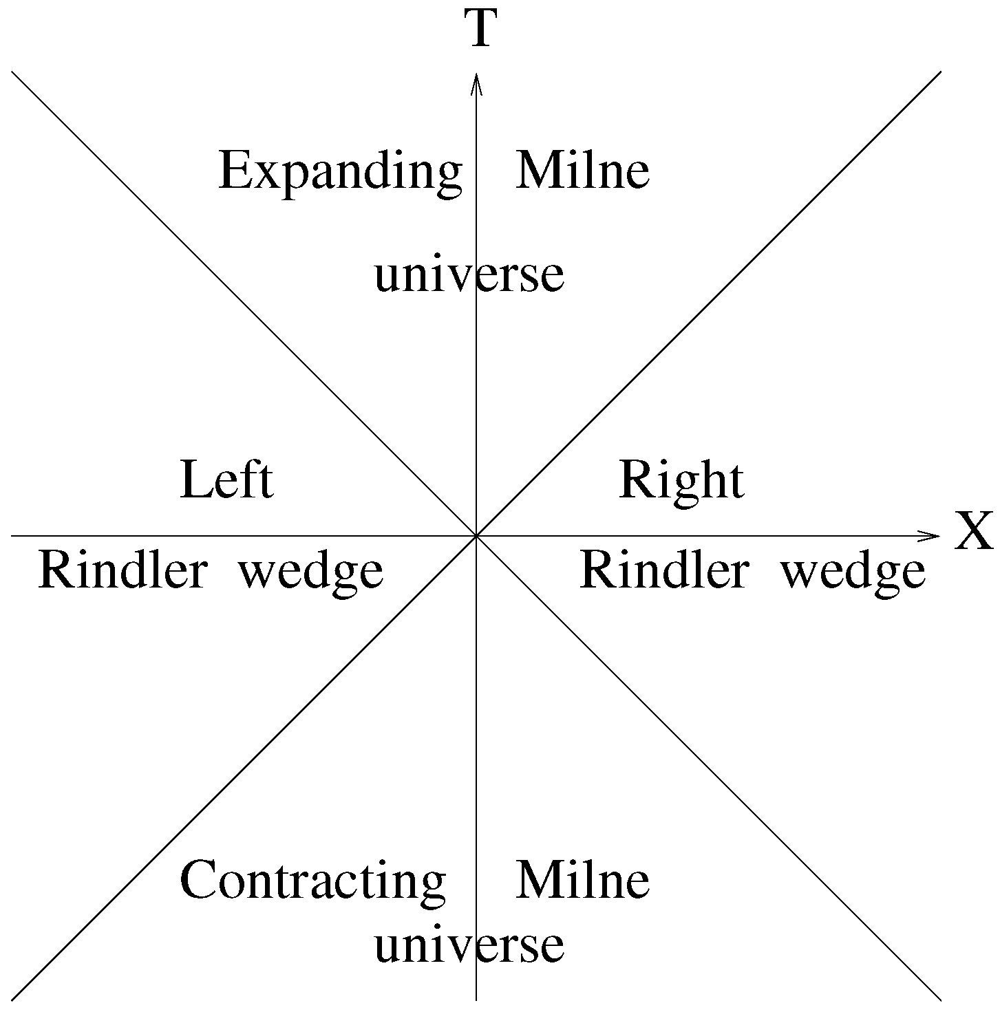
Figure 2 summarizes our findings. It is interesting to note that the above discussion of the Milne (or Rindler) space-time extension closely resembles the celebrated Kruskal extension of the Schwarzschild space-time [20,106,107]. More precisely, the expanding Milne universe corresponds to the black hole region of the Kruskal diagram, the contracting Milne universe corresponds to the white hole region, and the Rindler space-time corresponds to outer Schwarzschild regions [20].
Figure 2.
The patches of the Minkowski space-time covered by the Milne and Rindler metrics.
What is the physical meaning of the Rindler coordinates? Inspired by the Milne interpretation outlined above, let us consider a set of Rindler fundamental observers which are at rest in the Rindler space-time having constant spatial coordinates. The line of simultaneity for an arbitrary event at the worldline of a Rindler observer is the set of events that are simultaneous with P in the inertial instantaneous rest frame of the Rindler observer at P. As is fixed, this instantaneous rest frame moves with the the Minkowski velocity (in the private space of the Big Bang event)
Therefore, according to the Lorentz transformations, in the instantaneous rest frame the event P has the time coordinate , what means that it is simultaneous with the Big Bang event. As both the Rindler observer and the point on its worldline were arbitrary, we come to an amusing conclusion that the Big Bang event is simultaneous with every event on the worldline of every Rindler observer. In other words, the space axes of the fundamental Rindler observers all pass through the Big Bang event. In comparison, the defining characteristic property of the Milne observers is that all their time axes pass through the Big Bang event. This interchange of space and time makes a big difference: the Rindler observers cannot be inertial because the space axes of the inertial observer are all parallel to each other and thus cannot cross at the origin.
From Equation (84) the acceleration of the Rindler observer is
On the other hand, differentiating the velocity addition formula
and using , we get
As we see from Equation (87), the Rindler observers in the private space of the Big Bang event move with the constant proper acceleration which is inversely proportional to their Rindler coordinate and approaches the infinity for observers near the Big Bang, .
Equation (84) shows that at Rindler time all Rindler observers have the same rapidity . In fact the rapidity is the most natural (dimensionless) time coordinate in the Rindler space-time. The Rindler metric expressed in terms of the rapidity ψ does not contain an arbitrary constant g. Similarly, in the Milne space-time the rapidity is the most natural (dimensionless) spatial coordinate.
What is the origin of the constant g? The fact that Rindler observers share their lines of simultaneity enables us to define global synchronization in the Rindler space-time: we can simply pick out an arbitrary Rindler observer with the spatial coordinate and declare its proper time to be the coordinate time . But the proper time of the observer with the spatial coordinate is
Comparing with Equation (83), we see that
We have chosen to define synchronization for the selected observer, and hence, , so that g is the proper acceleration of this observer. Therefore, the freedom to use an arbitrary constant in description of the Rindler space-time is the freedom to select any Rindler observer to define global synchronization and hence, the coordinate time . For Rindler observers other than the selected one, the proper time will not coincide with the coordinate time but will be proportional to it, as Equation (88) shows.
As we see, the Rindler space-time is a part of the Minkowski space-time as viewed by a set of non-inertial observers whose constant proper accelerations are adjusted in such a way that their lines of simultaneity all pass through one event (Big Bang). Further details and a lucid discussion of the physical meaning of Rindler coordinates can be found in [108].
Note that in the four-dimensional space-time radially moving Rindler observers define spherical Rindler coordinates as follows [109]
They cover the whole external part of the Big Bang’s light-cone (subdivision into Rindler wedges arises only in the -dimensional space-time) where the induced metric is
5. St. Augustine’s Objects
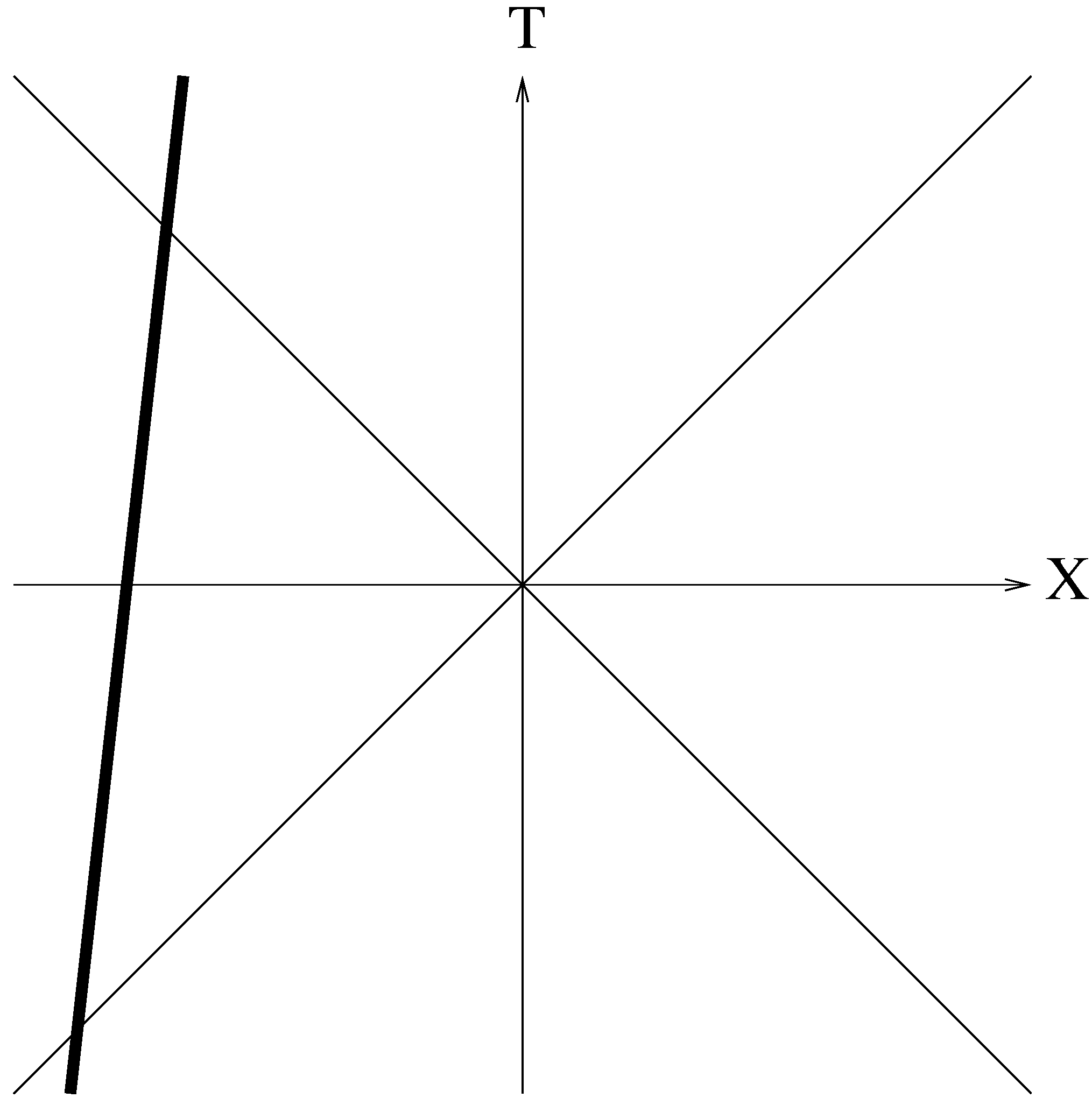
Both Milne and Rindler fundamental observers may not suspect that their space-times are just some parts of a bigger entity – the Minkowski space-time. However, we know that this is the case. A legitimate question then is whether Milne and Rindler parts of the Minkowski space-time can exchange material objects. As far as the space-time itself is concerned, the only restriction is causality, because the Minkowski space-time is not singular. Thus, naively, material objects from other parts of the Minkowski space-time can penetrate expanding Milne universe. One timelike world line of this kind is shown on Figure 3. We will call such objects, maybe rather frivolously, the St. Augustine’s objects.
Figure 3.
The world line of the St. Augustine’s object drawn here as a thick line.

St. Augustine of Hippo was the most influential philosopher who pondered on the nature of time. “What then is time? If no one asks me, I know what it is. If I wish to explain it to him who asks, I do not know” —ruminates he in his Confessions [110]. St. Augustine’s version of the modern question what was going on before the big bang sounds like this: “What was God doing before He made heaven and earth?”. St. Augustine overcomes his own temptation to laugh at the question and give a jesting answer: “He was preparing hell for those who pry into mysteries.” Instead he comes to an answer which strikingly resonates with the modern day ideas about space-time and that the universe was created by quantum tunneling from a state with no classical space time [111,112]. Namely, in City of God [113] he comes to the conclusion that “time does not exist without some movement and transition” and this is what distinguishes eternity and time. His main inference then is that “the world was made, not in time, but simultaneously with time”. In modern words, time itself was created by the Big Bang and the question what was before the Big Bang is meaningless, it is like asking what is to the north to the North Pole [114].
However St. Augustine’s brilliant insight that the time was created simultaneously with the material world should be taken with a grain of salt, because the use of the word “create” may imply that there was some concept of time even at the epoch when time was still not existing [115,116]. The Milne model provides a ready resolution of this dilemma.
As we know, there are two notions of time in the Milne model. The public time is determined by an expanding substratum of fundamental particles. Space-like hypersurfaces orthogonal to the world lines of these fundamental particles define a public space. The public time is the proper time along world lines of the fundamental particles and this cosmic time in a sense labels the series of the space-like hypersurfaces. Therefore, the public time is created by the Big Bang and it is really meaningless to ask what happened before the public time zero.
However, to any inertial fundamental particle in the Milne model we can attach the usual Minkowski frame and thus define the private time of this observer. If there are fundamental observers whose world lines begin not at the Big Bang but in the preceding contracting phase, we can use the private time of such observers supposing that they survived during the Big Bang, to make the question of what happened before the Big Bang obviously meaningful.
The central question, therefore, is whether material objects can cross the boundaries (the future light-cone of the Big Bang event) of the expanding Milne universe. This question is not a trivial one, because the density of the fundamental observers, as we have seen above, becomes infinite at these boundaries, as a result of the cosmological principle.
Milne himself was well aware of this problem. However, he considers the question what is outside the sphere in the private space as meaningless based on the following arguments [93].
Milne observers inside the sphere cannot observe any object outside, because infinite density of fundamental particles on this sphere serves as a curtain obscuring the vision and precludes any window into outer space in any direction. Therefore, only objects which were overtaken by the expanding frontier and appeared inside the sphere can be observed. For inhabitants of the Milne universe the St. Augustine objects would suddenly appear to observation in an act of creation. More precisely, from the point of view of public time, such objects are just a part of the Big Bang initial conditions.
However, Milne thinks that the infinite density of fundamental particles on the expanding frontier can lead to the infinite number of collisions between the St. Augustine object and the fundamental particles, thus, not allowing the St. Augustine object to penetrate the boundary. In fact, not the infinite density by itself is crucial in this argument, but a particular form of the density function Equation (63), which implies that the total number of particles in any thin layer including the boundary is infinite. Milne concludes: “such objects never come, and never can come, into interaction with observable members of the given system. They may, mathematically described, tend to be swept up by the expanding frontier, but they never penetrate it. Penetration would be a logical self-inconsistency of description of the whole system” [93].
But can the ideal Milne universe actually be realized? The infinite number of needed fundamental particles and the initial (in cosmic time) singularity of infinite density, implied by Equation (67), speak against such a possibility. Another argument against the realizability of the ideal Milne universe can be obtained by considering quantum fields in the Milne universe.
In analogy with Equation (78), let us define the dimensionfull temporal and spatial Milne coordinates:
They are related to the Minkowski coordinates through:
The Milne metric Equation (72) in terms of these coordinates takes conformally flat form
In contrast to the cosmic time t whose range is , the range of the conformal Milne time (as well as of the spatial coordinate ) is the whole real axis from to .
Free scalar field with mass in the Milne universe satisfies the covariant Klein-Gordon equation
where the covariant d’Alembertian (Laplace-Beltrami operator) has the form
For scalar Φ and vector fields the covariant derivative is defined as follows [20]
where the connection coefficients (Christoffel symbols) are
Therefore,
and
For the metric Equation (92), the only non-zero components of the metric tensor are
Then
and it can be easily checked that the second term in Equation (95) equals to zero. Finally,
and the Klein-Gordon Equation (93) takes the form
We can separate variables, taking , and get
where , and λ is some constant. Only if this constant is negative, , the solution does not grow exponentially. Then the equation for is
This equation is formally identical to the s-wave radial Schrödinger equation for an exponential potential with well known solution [117]. Namely, in terms of the cosmic time , Equation (97) takes the form
which is Bessel’s equation (of pure imaginary order) with the general solution [117]
where and are arbitrary constants.
Therefore, to get the positive-frequency mode (which behaves as ) in the asymptotic past (in Milne conformal time ), we must take . The second constant, , can be fixed by normalizing the mode using the covariant norm [119,120]
where is the determinant of the metric tensor, Σ is a spacelike hypersurface with being the unit timelike vector normal to it, and is the invariant (proper) volume element in this hypersurface. Using the Gauss’ theorem for curved manifolds [119,
it can be proved [120,121] that the scalar product is independent of the choice of spacelike surface Σ provided and are solutions of the Klein-Gordon Equation (93) that vanish sufficiently quickly at spatial infinity. Indeed, let V be the four-volume whose boundary consists of non-intersecting spacelike hypersurfaces , and, possibly, by timelike boundaries at spatial infinity on which . Then we have
where . But as and are solutions of the Klein-Gordon Equation (93), then:
Therefore,
Let us specify the scalar product Equation (100) for our case of two-dimensional Milne space-time with the metric Equation (92). The convenient choice of Σ is the spacelike hyperbola defined by the condition . Then the proper line element in Σ is , and the unit vector (normalized according to the metric Equation (92)) is . Therefore, the scalar product takes the form
Now we can determine the constant . In fact, using , the Wronskian relation [118]
and the normalization (for the positive-frequency modes)
we find that the normalized mode, which behaves as of pure positive frequency in the asymptotic past, has the form
In the asymptotic future, , the cosmic time t also tends to infinity and we should use the following asymptotic behavior [118]: when , then
Using Equation (103), it can be verified that the combinations Equation (99) that correspond to the positive and negative frequency behavior () in asymptotic future are, respectively, the Hankel functions and , defined by
Using the Wronskian relation [118]
we find that the normalized modes, corresponding to the positive and negative frequencies in the asymptotic future, have the form
Note that the negative frequency mode has the negative norm:
Equation (102), Equation (104) and Equation (105) imply the relation
which shows that the pure positive-frequency mode in the asymptotic past evolves into a superposition of positive- and negative-frequency modes and of the asymptotic future [122]. The standard interpretation [119] of this fact is that the time-dependent background metric leads to a pair production with the averaged number density of produced pairs in the k-mode
The problem, however, is that, if we consider the Milne universe as just a re-parametrization of the part of Minkowski space-time, the time dependence of the background metric is just a coordinate artifact, not related to the real presence of a variable gravitational field, and, hence, no particle production is expected [122]. The crux of the problem can be traced back to the definition of the initial vacuum state [123].
Suppose we have a nonzero rate R of particle production due to time-variable background metric. To measure precisely the number of particles in some volume, the measurement duration must be sufficiently small, namely such that . However, the smaller is the measurement time , the greater is the uncertainty in energy , and due to the possibility of temporary creation of virtual particle pairs, the number of particles will become uncertain by the amount . Therefore, over a time interval , the total uncertainty in the number of particles is [119,124]
The optimum is reached at
which gives the following minimum inherent uncertainty of the number of particles:
This simple computation indicates that in an adiabatic region, where the Hubble parameter is small (the scale factor varies slowly and hence is expected to be small), the concept of particles, and hence of the vacuum state, is a well defined concept. For the Milne universe . Therefore, the vacuum state is well defined in remote future. However, the region of the Milne space-time near the initial singularity is not an adiabatic region and we do not have a natural well defined vacuum state there. We can use (as we have, in fact, done above) the conformal time and quantum states that contain only positive frequencies with respect to this conformal time, when , to define the initial vacuum state in this region. Such conformal vacuum state is, of course, not adiabatic and its use in the role of the initial vacuum state may seem as a somewhat arbitrary choice [123]. Nevertheless, this choice is justified in the path-integral formulation, where it corresponds to the natural restriction of the paths summed to those that lie inside the future light-cone of the initial singularity (the Big Bang event) [125].
However, this restriction is natural only when the initial singularity is real and not a coordinate artifact, as in the case of the naive interpretation of the Milne model.
When , we have the following integral representations of the Hankel functions [126]:
After changing the integration variable u in the above integrals respectively to , Equation (109) take the form
where and . As we see, is a superposition of positive frequency Minkowski plane waves with different rapidities , while is a superposition of negative frequency Minkowski plane waves [119,127]. Of course, instead of the rapidity , we can use the momentum as an integration variable [123]:
The integral representations Equation (110), or Equation (111) define a natural analytic continuations of and on the whole Minkowski space-time [123,127] and, of course, these analytic continuations pick up a privileged vacuum state corresponding to no particle production. If we consider the Milne universe as a part of Minkowski space-time, this choice of the vacuum state is the most natural. However, from the point of view of the inside observers of the Milne universe, it may appear rather contrived and will require subtle arguments to justify it from the inside perspective [123].
An other possibility is given by considering the Milne universe as a limiting case of some nonsingular space-time whose metric differs from the Milne-Rindler metric only in the narrow transition region around the Big-Bang light-cone [128]. In this case the particle production can be related to the nonzero time-variable curvature of the space-time (a real time dependent gravitational field) in the transition region. One can imagine that this effect of particle production can take place even in the limit of zero width of the transition region, however such a situation will require a physically unrealistic sources of infinite power on the Milne universe singular boundary [128]. Of course, this picture is in accord with the infinite density of the Milne observers at the boundary, but these infinities make the construction of the ideal Milne universe with impenetrable boundaries (for example, in hydrodynamical laboratory experiments to mimic an arbitrary FRW space-time by relativistic acoustic geometry [129]) impossible. Therefore, any realistic approximation to the ideal Milne universe is expected to have boundaries penetrable for St. Augustine’s objects.
Now we assume that the same is true to our real universe: the initial singularity is only an unrealistic idealization and in realistic settings it is traversable for St. Augustine’s objects. As we expect that the initial density at the Big Bang was nevertheless very high, we assume that only black holes as St. Augustine’s objects can survive such a dramatic event. Therefore, we conclude that it is possible to have some amount of black hole population, moving relativistically with respect to the nearby Hubble flow at high redshifts, as a part of the Big Bang initial conditions. If the amount of such St. Augustine’s objects is small, they cannot significantly change the dynamics of the universe and spoil the successful predictions of the standard cosmological model.
Let us sketch, from the Milne model perspective, how St. Augustine’s objects in the role of quasars can offer an explanation of some above mentioned mysteries.
Let us begin with the time non-dilation mystery. It is expected that the most radiation from quasars comes from the ambient matter heated by shock waves when St. Augustine’s black hole moves relativistically through this matter. Therefore, the associated red-shifts will be truly cosmological as originated from the matter which participates in the Hubble flow. On the other hand, any internal variability related to the black hole itself (for example, due to instabilities in the accretion disc) will not be time-dilated if the St. Augustine’s object is nearly motionless with respect to us in our private space.
The mystery related to the origin of supermassive black holes also becomes less acute. Indeed, St. Augustine’s black holes might already have been sufficiently massive upon entering our universe. Moreover, initially St. Augustine’s black hole moves ultrarelativistically through ambient matter and extremely high value of its gamma-factor drives it into the fast growing mode [130].
Such high gamma-factors are considered as unrealistic for primordial black holes in the early universe [130], but for St. Augustine’s black holes this is just what is expected most naturally from anthropic principle. Indeed, if we assume that the relativistic velocity of the St. Augustine’s black hole with respect to ambient Hubble flow matter is essential for triggering the quasar activity, an immediate anthropic principle type consequence would be that we are not a typical observer but rather a special one, namely the one which is nearly at rest with respect to potential St. Augustine’s objects population, because otherwise the existence of nearby quasars would make development of intelligent life impossible. At that, of course, we have implicitly assumed that St. Augustine’s objects population indeed define a reasonable standard of rest. To make sure that this is a plausible supposition, imagine an analog FRW space-time created in a hydrodynamical laboratory experiment, as advocated in [129]. Then the vessel in which an expanding relativistic fluid mimics the FRW universe provides a natural standard of rest and various residual gas molecules, as candidate St. Augustine’s objects for this simulated FRW universe, approximately can be considered as nearly at rest with respect to the vessel from the point of view of participants of the relativistic flow.
As relative velocities of St. Augustine’s black holes with respect to ambient Hubble flow matter increase with redshift, it is expected that high redshift quasars will be more luminous than low redshift quasars. Therefore, the observed evolution of quasar luminosity over redshifts is no longer mysterious but finds its explanation if quasars are related to St. Augustine’s objects.
The shock wave, which surely accompanies the motion of the St. Augustine’s black holes through ambient matter, is expected to trigger intense star formation in this ambient matter and hence increase the expected supernovae rates. Thus, it becomes possible to explain the appearance of unusually young chemically mature galaxies around high-redshift quasars.
Probably, shock waves caused by St. Augustine’s objects can give a clue also to the most mysterious of paradoxes related to quasars: alleged correlations of objects that have vastly different redshifts. Schematically this is explained on Figure 4.
At a space-time point A a St. Augustine’s object enters into the Milne universe and at the present time we, situated at the point E, observe the light emitted by the corresponding quasar at point C. The accompanying shock wave propagates along the world line and at a point B triggers the formation of the seed of future galaxy which sends to us the light from the point D when it is already formed. As a result, we observe a distant quasar and much closer galaxy aligned, and this alignment is really not by a chance, but due to above described fancy causal relation between them.
It can be expected that the shock wave will give birth not to one but to several galaxies along its world line. Therefore, we expect chains of galaxies with different redshifts all aligned with a quasar. Remarkably, according to Arp [68], there are actually many examples of such chains of galaxies throughout extragalactic space. In fact this effect is so pronounced that it led Victor Ambartsumian in 1958 to the exotic idea that new galaxies are formed through the ejection from older active galaxies [70]. He came to this idea by simply looking at pictures of galaxies. Eight years later Arp came to the same conclusion by inspecting much more detailed and significantly better quality images of peculiar galaxies [131]. Ambartsumian presented his conclusions at the prestigious Solvay conference. However, “this select group of the best known scientists in the world had either been completely baffled or laughed privately at these crazy ideas” [131]. Interestingly enough, the paradigm of St. Augustine’s objects reconciles Ambartsumian’s and Arp’s exotic idea that galaxies beget galaxies with the standard cosmological interpretation of redshifts in a manner which does not undermine the standard theory of galaxy formation for the bulk of galaxy population, if the number of the St. Augustine’s objects is small enough.
Figure 4.
A schematic mechanism explaining correlations of objects that have vastly different redshifts. See text for details.
Figure 4.
A schematic mechanism explaining correlations of objects that have vastly different redshifts. See text for details.

As the last bonus, the paradigm of St. Augustine’s objects also explains why the observation of an apparent superluminal motion in quasars is not a relatively rare phenomenon. In public space, St. Augustine’s objects move relativistically nearly towards us so that the associated blue-shift nearly compensates the cosmological redshift for any internal variation of intensity. As a by product, relative motion of any quasar-related two radio emitting blobs will be with a high probability radial and hence can lead to the apparent superluminal motion.
6. Concluding Remarks
We have heavily used the Milne model in this article to justify our suppositions. It is time to ask what are the relations of this model with reality. We introduced the Milne metric as a metric of an empty FRW universe. The present density of matter is rather low in terms of the critical density. Therefore, probably, it is not surprising that the Milne metric describes some aspects of the present day universe quite satisfactorily. Namely, curiously the Milne model explains supernovae observations rather well without requiring any dark energy [132,133]. The standard concordance ΛCDM model with positive cosmological constant, of course, provides a better fit and, as expected, an empty universe is not its viable alternative. Nevertheless, “the Milne model has great pedagogical value, elucidating the kinematic aspect of the universe’s expansion” [133].
However, in fact, Milne’s aspiration was significantly more ambitious than just providing late time approximate description of FRW cosmology in terms of special relativity. Milne believed that some very general rational and at the same time aesthetic principles were at the foundations of the observed order and regularities in the universe. His approach, named kinematic relativity [94], was conceived as a rival theory to the standard relativistic cosmology. Milne’s aim was “to deduce as much as possible merely from the cosmological principle and the basic properties of space, time and the propagation of light” [134] revealed by special relativity.
Milne’s unorthodox methodology triggered a heated debate involving the most eminent cosmologists of the time [135,136,137]. When the kinematic relativity was first developed “it met great hostility and was criticized very severely, often unjustly, and sometimes frivolously” [134].
In retrospect, the influence of Milne on the development of modern cosmology was very substantial and he inspired others, in particular Robertson and Walker, in shaping fundamental concepts of modern cosmology [135,136,137]. However, as for the kinematic relativity, very little work has been done on it since the death of Milne and the theory has been left “in a curiously unfinished state” [134]. Walker showed [138,139] that Milne’s cosmological construction, if described in terms of geometry, was fundamentally different from that of general relativity and, in general, such a description requires Finsler geometry, a generalization of Riemannian geometry (for applications of Finsler geometry see, for example, [140,141]). Although we feel that the Finslerian perspective of the Milne model was not sufficiently explored, at present the Milne model cannot be considered as a viable alternative to the standard relativistic cosmology, of course. Therefore, in the spirit of this paper we can use it as only a source of inspiration and not a solid ground to justify the introduction of the St. Augustine’s objects. Can we find a support for them in more mainstream theories?
In non-empty FRW cosmological models we cannot define global inertial frames and thus, we cannot introduce private time like Milne did. However, a plausible generalization of the concept of private time can be envisaged in the general case as well thanks to the fact that Weyl Tensor for all FRW Cosmological metrics vanishes and thus all FRW space-times are conformally flat [142,143]. Suitably defined conformal time can serve as a substitute of private time. For example, in the case of the flat FRW metric we can introduce conformal time-coordinate T and conformal radial coordinate R in the following way [143]
where
with arbitrary . Substituting the inverse transformations
into Equation (4) and taking into account that according to Equation (113) , we find that the metric Equation (4) (with ) indeed takes the conformally flat form:
According to Equation (112), region is mapped onto the region , while the region —onto the region . As in the case of private space and time in the Milne model, the FRW universe coordinates occupy only a quarter of the plane and this circumstance hints at a possibility that the FRW universe might be just a part of some bigger entity. Let us note, however, that the conformal coordinates considered are not exact analogues of the Milne’s private time and private space. In particular, transformations Equation (112) are singular at the light-cone .
Another analogue of the Milne foliation is the Rindler’s foliation of a non-empty FRW space-time [96] by spacelike slices of finite volume. Rindler showed that, just like the Milne universe, “every open big-bang FRW universe can be regarded as an expanding finite-volume ball of matter, springing from zero volume” [96]. This feature of FRW space-time becomes particularly clear from the multi-dimensional perspective [96]. It is well known that any four-dimensional space-time can be locally embedded (immersed) in a ten-dimensional flat pseudo-Euclidean space [144]. Because of the high degree of symmetry of the FRW space-time, its embedding is possible even in a five-dimensional pseudo-Euclidean space [145]. Namely, the embedding of a spatially flat FRW spacetime
into the five-dimensional Minkowski space is defined by relations [145]:
where and α is a constant with the dimension of length.
In the right part of Equation (118), the cosmic time t can be considered as a function of because, according to Equation (117),
Therefore, Equation (118) and Equation (119) define a hyper-surface in the five-dimensional Minkowski space. For example, in the radiation dominated universe with some τ, and the Equation (118), defining the hyper-surface, takes the form (in the case )
In fact, the FRW space-time corresponds to only a portion of this hyper-surface, because according to Equation (119) we must have .
As we see, a multi-dimensional perspective allows to consider a non-empty FRW universe as a part of a bigger entity and the overall picture is similar to the one in the Milne model that led us to the St. Augustine’s objects hypothesis.
It is worth mentioning that extra-dimensional models were very popular in the last decade. In such models, an ambient space is not the Minkowski space but has more complex geometry. The universe as a thin shell expanding in a five-dimensional space with so called non-factorizable warped geometry was first considered by Gogberashvili in [146], and such models with warped extra dimensions became very popular after the Randall and Sundrum paper [147]. Other popular extra-dimensional models are Kaluza-Klein type models with compactified extra-dimensions [148]. It is assumed that all Standard Model particles are confined to the four-dimensional hyper-surface, a brane, in a higher dimensional space. Gravity, on the contrary, can freely propagate in the bulk thus explaining the weakness of the gravitational interactions between the brane confined particles by accompanying spreading of gravitational flux into the large volume of the extra dimensions. In our terminology, gravitons are St. Augustine’s objects in these models, and who knows what other type of St. Augustine’s objects are lurking in the bulk.
Gravitons also play the role of St. Augustine’s objects in Penrose’s conformal cyclic cosmology [149]. Gravitational waves emitted in close encounters between super-massive black holes in the last contracting phase of the previous aeon can propagate into the next aeon giving rise to fancy concentric circular rings with slightly different temperature on the Cosmic microwave background sky [149].
Finally, let us mention the so called Ekpyrotic cosmology in which the Big Bang is associated not with a singularity but with a collision of two branes in the extra-dimensional bulk [150]. As a result, cyclic model of the universe can be constructed in which there is an endless sequence of cosmic epochs of expansion and contraction [151]. Black holes as possible St. Augustine’s objects in such cyclic scenarios, surviving a bounce of the Big Crunch-Big Bang transition, are discussed in [152]. Interestingly, modern attempts to discuss sailing through the big crunch-big bang transition involves the (compactified) Milne universe in an essential way [122,153]. Milne’s influence on the modern cosmology is ongoing!
Acknowledgements
The work of Zurab K. Silagadze is supported by the Ministry of Education and Science of the Russian Federation and in part by Russian Federation President Grant for the support of scientific schools NSh-2479.2014.2 and by RFBR grant 13-02-00418-a.
References and Notes
- Tyutchev, F.I. A Spring Storm. 1828. Available online: http://www.ruthenia.ru/tiutcheviana/publications/trans/springstorm.html (accessed on 28 September 2015).
- Hawkins, M.R.S. On time dilation in quasar light curves. Mon. Not. Roy. Astron. Soc. 2010, 405, 1940–1946. [Google Scholar] [CrossRef]
- Veltman, M. Diagrammatica; Cambridge University Press: Cambridge, UK, 1995. [Google Scholar]
- Lineweaver, C.H.; Davis, T.M. Misconceptions about the Big Bang. Sci. Am. 2005, 292, 36–45. [Google Scholar] [CrossRef]
- Francis, M.J.; Barnes, L.A.; James, J.B.; Lewis, G.F. Expanding Space: The Root of all Evil? Publ. Astron. Soc. Austral. 2007, 24, 95–102. [Google Scholar] [CrossRef]
- Peacock, J.A. A diatribe on expanding space. 2008; arXiv:0809.4573, [astro-ph]. [Google Scholar]
- Braeck, S.; Elgarøy, Ø. A physical interpretation of Hubble’s law and the cosmological redshift from the perspective of a static observer. Gen. Rel. Grav. 2012, 44, 2603–2610. [Google Scholar] [CrossRef]
- Cook, R.J.; Burns, M.S. Interpretation of the Cosmological Metric. Am. J. Phys. 2009, 77, 59–66. [Google Scholar] [CrossRef]
- Chodorowski, M. A direct consequence of the expansion of space? Mon. Not. Roy. Astron. Soc. 2007, 378, 239–244. [Google Scholar] [CrossRef]
- Melia, F. Cosmological redshift in Friedmann-Robertson-Walker metrics with constant space-time curvature. Mon. Not. Roy. Astron. Soc. 2012, 422, 1418–1424. [Google Scholar] [CrossRef]
- Grøn, Ø.; Elgarøy, Ø. Is space expanding in the Friedmann universe models? Am. J. Phys. 2007, 75, 151–157. [Google Scholar]
- Roukema, B.F. There was movement that was stationary, for the four-velocity had passed around. Mon. Not. Roy. Astron. Soc. 2010, 404, 318–324. [Google Scholar] [CrossRef]
- Hartnett, J.G. Is the universe really expanding? 2011; arXiv:1107.2485, [physics.gen-ph]. [Google Scholar]
- Lopez-Corredoira, M. Tests for the Expansion of the Universe. 2015; arXiv:1501.01487, [astro-ph.CO]. [Google Scholar]
- Mitra, A. When can an “Expanding Universe” look “Static” and vice versa: A comprehensive study. Int. J. Mod. Phys. D 2015, 24, 1550032. [Google Scholar] [CrossRef]
- Minkowski, H. Space and Time. In The Principle of Relativity: A Collection of Original Memoirs on the Special and General Theory of Relativity; Lorentz, H.A., Einstein, A., Minkowski, H., Weyl, H., Eds.; Dover Publications: New York, USA, 1952; p. 75. [Google Scholar]
- Wigner, E.P. Relativistic invariance and quantum phenomena. Rev. Mod. Phys. 1957, 29, 255–268. [Google Scholar] [CrossRef]
- Carroll, S.M. Lecture notes on general relativity. 1997; arXiv:gr-qc/9712019. [Google Scholar]
- Giulini, D. Does cosmological expansion affect local physics? 2013; arXiv:1306.0374, [gr-qc]. [Google Scholar]
- Rindler, W. Relativity: Special, General and Cosmological; Oxford University Press: Oxford, UK, 2001. [Google Scholar]
- Herranz, F.J.; Ortega, R.; Santander, M. Trigonometry of spacetimes: A new self-dual approach to a curvature/signature (in)dependent trigonometry. J. Phys. A 2000, 33, 4525–4551. [Google Scholar] [CrossRef]
- Ballesteros, A.; Herranz, F.J.; del Olmo, M.A.; Santander, M. Quantum structure of the motion groups of the two-dimensional Cayley-Klein geometries. J. Phys. A 1993, 26, 5801–5823. [Google Scholar] [CrossRef]
- Narlikar, J.V. An Introduction to Cosmology; Cambridge University Press: Cambridge, UK, 1993. [Google Scholar]
- “The great tragedy of Science: the slaying of a beautiful hypothesis by an ugly fact” (Thomas Henry Huxley, 1870). Qouted in The Yale Book of Quotations; Shapiro, F. R.; Epstein, J. (Eds.) Yale University Press: London, UK, 2006; p. 379.
- Zee, A. Einstein Gravity in a Nutshell; Princeton University Press: Princeton, NJ, USA, 2013. [Google Scholar]
- Moschella, U. The de Sitter and anti-de Sitter Sightseeing Tour. In Einstein, 1905–2005, Poincaré Seminar 2005; Damour, T., Darrigol, O., Duplantier, B., Rivasseau, V., Eds.; Birkhäuser Verlag: Basel, Switzerland, 2006; pp. 120–133. [Google Scholar]
- Blondin, S.; Davis, T.M.; Krisciunas, K.; Schmidt, B.P.; Sollerman, J.; Wood-Vasey, W.M.; Becker, A.C.; Challis, P.; Clocchiatti, A.; Damke, G.; et al. Time Dilation in Type Ia Supernova Spectra at High Redshift. Astrophys. J. 2008, 682, 724–736. [Google Scholar] [CrossRef]
- Wilson, O.C. Possible Applications of Supernovae to the Study of the Nebular Red Shifts. Astrophys. J. 1939, 90, 634–636. [Google Scholar] [CrossRef]
- Crawford, D.F. No Evidence of Time Dilation in Gamma-Ray Burst Data. 2009; arXiv:0901.4169, [astro-ph.CO]. [Google Scholar]
- Kocevski, D.; Petrosian, V. On The Lack of Time Dilation Signatures in Gamma-ray Burst Light Curves. Astrophys. J. 2013, 765, 116. [Google Scholar] [CrossRef]
- Littlejohns, O.M.; Butler, N.R. Investigating signatures of cosmological time dilation in duration measures of prompt gamma-ray burst light curves. Mon. Not. Roy. Astron. Soc. 2014, 444, 3948–3960. [Google Scholar] [CrossRef]
- Zhang, F.W.; Fan, Y.Z.; Shao, L.; Wei, D.M. Cosmological Time Dilation in Durations of Swift Long Gamma-Ray Bursts. Astrophys. J. 2013, 778, L11. [Google Scholar] [CrossRef]
- Ellis, G.F.R. Contributions of K. Gödel to relativity and cosmology. Lect. Notes Log. 1996, 6, 34–49. [Google Scholar]
- Lanczos, K. On a Stationary Cosmology in the Sense of Einstein’s Theory of Gravitation. Gen. Rel. Grav. 1997, 29, 363–399. [Google Scholar] [CrossRef]
- Van Stockum, W.J. The gravitational field of a distribution of particles rotating around an axis of symmetry. Proc. Roy. Soc. Edinburgh 1937, 57, 135–154. [Google Scholar] [CrossRef]
- Hawking, S. The Existence of cosmic time functions. Proc. Roy. Soc. Lond. A 1968, 308, 433–435. [Google Scholar] [CrossRef]
- Geroch, R.P. General relativity in the large. Gen. Rel. Grav. 1971, 2, 61–74. [Google Scholar] [CrossRef]
- Geroch, R.; Horowitz, G.T. Global structure of spacetimes. In General Relativity: An Einstein Centenary Survey; Hawking, S., Isreal, W., Eds.; Cambridge University Press: Cambridge, UK, 1979; pp. 212–293. [Google Scholar]
- Minguzzi, E. On the global existence of time. Int. J. Mod. Phys. D 2009, 18, 2135–2144. [Google Scholar] [CrossRef]
- Weyl, H. Raum, Zeit, Materie, 5th ed.; Springer: Berlin, Germany, 1923. [Google Scholar]
- Rugh, S.E.; Zinkernagel, H. Weyl’s principle, cosmic time and quantum fundamentalism. 2010; arXiv:1006.5848, [gr-qc]. [Google Scholar]
- Kellermann, K.I. The Discovery of Quasars. Bull. Astron. Soc. India 2013, 41, 1–17. [Google Scholar]
- D’Onofrio, M.; Marziani, P.; Sulentic, J.W.; Collin, S.; Setti, G.; Gaskell, M.; Wampler, J.; Elvis, M.; Pronik, I.; Pronik, V.; et al. Quasars in the Life of Astronomers. In Fifty Years of Quasars: From Early Observations and Ideas to Future Research; D’Onofrio, M., Marziani, P., Sulentic, J.W., Eds.; Springer: Heidelberg, Germany, 2012; pp. 11–90. [Google Scholar]
- Zel’dovich, Ya.B. The Fate of a Star and the Evolution of Gravitational Energy Upon Accretion. Sov. Phys. Dokl. 1964, 9, 195–197. [Google Scholar]
- Salpeter, E.E. Accretion of interstellar matter by massive objects. Astrophys. J. 1964, 140, 796–800. [Google Scholar] [CrossRef]
- Lynden-Bell, D. Galactic nuclei as collapsed old quasars. Nature 1969, 223, 690–694. [Google Scholar] [CrossRef]
- Ojha, R. Parsec-scale structure of quasars: dawn of the golden age? 2013; arXiv:1310.0875, [astro-ph.HE]. [Google Scholar]
- Antonucci, R. Astrophysics: Quasars still defy explanation. Nature 2013, 495, 165–167. [Google Scholar] [CrossRef] [PubMed]
- Lopez-Corredoira, M. Pending problems in QSOs. 2009; arXiv:0910.4297, [astro-ph.CO]. [Google Scholar]
- Kocsis, B.; Loeb, A. Menus for Feeding Black Holes. 2013; arXiv:1310.0815, [astro-ph.CO]. [Google Scholar]
- Frank, J.; King, A.; Raine, D. Accretion Power in Astrophysics; Cambridge University Press: Cambridge, UK, 2002. [Google Scholar]
- Peterson, B.M. An Introduction to Active Galactic Nuclei; Cambridge University Press: Cambridge, UK, 1997. [Google Scholar]
- Shen, Y. The Mass of Quasars. Bull. Astron. Soc. India 2013, 41, 61–115. [Google Scholar]
- Paczyńsky, B.; Wiita, P.J. Thick accretion disks and supercritical luminosities. Astron. Astrophys. 1980, 88, 23–31. [Google Scholar]
- Abramowicz, M.A. The Paczynski-Wiita potential: A step-by-step “derivation”. Astron. Astrophys. 2009, 500, 213–214. [Google Scholar] [CrossRef]
- Hobson, M.P.; Efstathiou, G.P.; Lasenby, A.N. General Relativity: An Introduction for Physicists; Cambridge University Press: Cambridge, UK, 2006. [Google Scholar]
- Alexander, D.M.; Hickox, R.C. What Drives the Growth of Black Holes? New Astron. Rev. 2012, 56, 93–121. [Google Scholar] [CrossRef]
- Narlikar, J.V. Alternative Views and Ideas. In Fifty Years of Quasars: From Early Observations and Ideas to Future Research; D’Onofrio, M., Marziani, P., Sulentic, J.W., Eds.; Springer: Heidelberg, Germany, 2012; p. 77. [Google Scholar]
- Finkelstein, S.L.; Papovich, C.; Dickinson, M.; Song, M.; Tilvi, V.; Koekemoer, A.M.; Finkelstein, K.D.; Mobasher, B.; Ferguson, H.C.; Giavalisco, M.; et al. A Rapidly Star-forming Galaxy 700 Million Years After the Big Bang at z=7.51. 2013; arXiv:1310.6031, [astro-ph.CO]. [Google Scholar]
- Jiang, L.; Fan, J.; Brandt, W.N.; Carilli, C.L.; Egami, E.; Hines, D.C.; Kurk, J.D.; Richards, G.T.; Shen, Y.; Strauss, M.A.; et al. Dust-free quasars in the early Universe. Nature 2010, 46, 380–383. [Google Scholar] [CrossRef] [PubMed]
- Jain, D.; Dev, A. Age of high redshift objects—a litmus test for the dark energy models. Phys. Lett. B 2006, 633, 436–440. [Google Scholar] [CrossRef]
- Friaca, A.; Alcaniz, J.; Lima, J.A.S. An old quasar in a young dark energy-dominated Universe? Mon. Not. Roy. Astron. Soc. 2005, 362, 1295–1300. [Google Scholar] [CrossRef]
- Kobayashi, C.; Umeda, H.; Nomoto, K.; Tominaga, N.; Ohkubo, T. Galactic chemical evolution: Carbon through Zinc. Astrophys. J. 2006, 653, 1145–1171. [Google Scholar] [CrossRef]
- Kobayashi, C.; Nomoto, K. The Role of Type Ia Supernovae in Chemical Evolution I: Lifetime of Type Ia Supernovae and Galactic Supernova Rates. Astrophys. J. 2009, 707, 1466–1484. [Google Scholar] [CrossRef]
- Wang, S.; Li, X.-D.; Li, M. Revisit of cosmic age problem. Phys. Rev. D 2010, 82, 103006. [Google Scholar] [CrossRef]
- Feige, B. Elliptic integrals for cosmological constant cosmologies. Astron. Nachr. 1992, 313, 139–163. [Google Scholar] [CrossRef]
- Thomas, R.C.; Kantowski, R. Age redshift relation for standard cosmology. Phys. Rev. D 2000, 62, 103507. [Google Scholar] [CrossRef]
- Arp, H. Quasars, Redshifts and Controversies; Cambridge University Press: Cambridge, UK, 1988. [Google Scholar]
- Kembhavi, A.K.; Narlikar, J.V. Quasars and Active Galactic Nuclei: An Introduction; Cambridge University Press: Cambridge, UK, 1999. [Google Scholar]
- Lopez-Corredoira, M. Apparent discordant redshift QSO-galaxy associations. 2009; arXiv:0901.4534, [astro-ph.CO]. [Google Scholar]
- Lopez-Corredoira, M.; Gutierrez, C.M. Two emission line objects with z > 0.2 in the optical filament apparently connecting the Seyfert galaxy NGC 7603 to its companion. Astron. Astrophys. 2002, 390, L15–L18. [Google Scholar] [CrossRef]
- Lopez-Corredoira, M.; Gutierrez, C.M. The Field surrounding NGC 7603: Cosmological or non-cosmological redshifts? Astron. Astrophys. 2004, 421, 407–423. [Google Scholar] [CrossRef]
- Blandford, R.D.; McKee, C.F.; Rees, M.J. Super-luminal expansion in extragalactic radio sources. Nature 1977, 267, 211–216. [Google Scholar] [CrossRef]
- Falla, D.F.; Floyd, M.J. Superluminal motion in astronomy. Eur. J. Phys. 2002, 23, 69–81. [Google Scholar] [CrossRef]
- Rees, M.J. Appearance of Relativistically Expanding Radio Sources. Nature 1966, 211, 468–470. [Google Scholar] [CrossRef]
- Kellermann, K.I.; Lister, M.L.; Homan, D.C.; Vermeulen, R.C.; Cohen, M.H.; Ros, E.; Kadler, M.; Zensus, J.A.; Kovalev, Y.Y. Sub-milliarcsecond imaging of quasars and Active Galactic Nuclei 3. Kinematics of parsec—scale radio jets. Astrophys. J. 2004, 609, 539–563. [Google Scholar] [CrossRef]
- Belchenko, Yu.I.; Gilev, E.A.; Silagadze, Z.K. Problems in Mechanics of Particles and Bodies; RCD: Moscow-Izhevsk, Russia, 2008. problem 2.6. (In Russian) [Google Scholar]
- Chodorowski, M.J. Superluminal apparent motions in distant radio sources. Am. J. Phys. 2005, 73, 639–643. [Google Scholar] [CrossRef]
- Narlikar, J.V.; Chitre, S.M. Faster-than-Light Motion in Quasars. J. Astrophys. Astron. 1984, 5, 495–506. [Google Scholar] [CrossRef]
- Lopez-Corredoira, M.; Perucho, M. Kinetic power of quasars and statistical excess of MOJAVE superluminal motions. Astron. Astrophys. 2012, 544, A56. [Google Scholar] [CrossRef]
- Ryle, M.; Longair, M.S. A Possible Method for Investigating the Evolution of Radio Galaxies. Mon. Not. Roy. Astron. Soc. 1967, 136, 123–140. [Google Scholar] [CrossRef]
- Urry, C.M.; Padovani, P. Unified schemes for radio-loud active galactic nuclei. Publ. Astron. Soc. Pac. 1995, 107, 803–845. [Google Scholar] [CrossRef]
- Rybicki, G.B.; Lightman, A.P. Radiative Processes in Astrophysics; Wiley-VCH: Weinheim, Germany, 2004. [Google Scholar]
- Landau, L.D.; Lifshitz, E.M. Course of Theoretical Physics, Vol. 2, The Classical Theory of Fields; Pergamon Press: Oxford, UK, 1975. [Google Scholar]
- Debbasch, F.; Rivet, J.-P.; van Leeuwen, W. Invariance of the relativistic one-particle distribution function. Phys. A 2001, 301, 181–195. [Google Scholar] [CrossRef] [Green Version]
- Treumann, R.A.; Nakamura, R.; Baumjohann, W. Relativistic transformation of phase-space distributions. Ann. Geophys. 2011, 29, 1259–1265. [Google Scholar] [CrossRef]
- Castor, J.I. Radiation Hydrodynamics; Cambridge University Press: Cambridge, UK, 2004. [Google Scholar]
- Bradt, H. Astrophysics Processes: The Physics of Astronomical Phenomena; Cambridge University Press: Cambridge, UK, 2008. [Google Scholar]
- Lind, K.R.; Blandford, R.D. Semidynamical models of radio jets—Relativistic beaming and source counts. Astrophys. J. 1985, 295, 358–367. [Google Scholar] [CrossRef]
- Bell, M.B. Doppler Boosting May Have Played No Significant Role in the Finding Surveys of Radio-Loud Quasars. Int. J. Astron. Astrophys. 2012, 2, 52–61. [Google Scholar] [CrossRef]
- Parker, R.H.; Wolnizer, P.W.; Nobes, C. (Eds.) Readings in True and Fair; Routledge: New York, NY, USA, 1996; p. 74.
- Milne, E.A. World-Structure and the Expansion of the Universe. Z. Astrophys. 1933, 6, 1–95. [Google Scholar] [CrossRef]
- Milne, E.A. Relativity, Gravitation and World-Structure; Oxford University Press: London, UK, 1935. [Google Scholar]
- Milne, E.A. Kinematic Relativity; Oxford University Press: London, UK, 1948. [Google Scholar]
- Milne, E.A. Modern Cosmology and the Christian Idea of God; Clarendon Press: Oxford, UK, 1952. [Google Scholar]
- Rindler, W. Finite foliations of open FRW universes and the point-like big bang. Phys. Lett. A 2000, 276, 52–58. [Google Scholar] [CrossRef]
- Sexl, R.U.; Urbantke, H.K. Relativity, Groups, Particles: Special Relativity and Relativistic Symmetry in Field and Particle Physics; Springer: Vienna, Austria, 2001; p. 38. [Google Scholar]
- Hearn, A.C. Reduce User’s Manual; Rand Corporation: Santa Monica, CA, USA, 1989. [Google Scholar]
- Silberstein, L. The Theory of Relativity; MacMillan: London, UK, 1914; p. 169. [Google Scholar]
- Ungar, A.A. Beyond the Einstein Addition Law and Its Gyroscopic Thomas Precession: The Theory of Gyrogroups and Gyrovector Spaces; Kluwer Academic Publishers: New York, NY, USA, 2002; p. 18. [Google Scholar]
- Robertson, H.P. On E.A.Milne’s Theory of World Structure. Z. Astrophys. 1933, 7, 153–166. [Google Scholar]
- Jammer, M. Concepts of Simultaneity: From Antiquity to Einstein and Beyond; Johns Hopkins University Press: Baltimore, MA, USA, 2006. [Google Scholar]
- Grøn, Ø. Big bang in a universe with infinite extension. Eur. J. Phys. 2006, 27, 561–565. [Google Scholar]
- Dirac, P.A.M. Forms of Relativistic Dynamics. Rev. Mod. Phys. 1949, 21, 392–399. [Google Scholar] [CrossRef]
- Czachor, M.; Wrzask, K. Automatic regularization by quantization in reducible representations of CCR: Point-form quantum optics with classical sources in the Milne universe. Int. J. Theor. Phys. 2009, 48, 2511–2549. [Google Scholar] [CrossRef]
- Wald, R.M. General Relativity; The university of Chicago Press: Chicago, IL, USA, 1984. [Google Scholar]
- Rindler, W. Kruskal Space and the Uniformly Accelerated Frame. Am. J. Phys. 1966, 34, 1174–1178. [Google Scholar] [CrossRef]
- Koks, D. Explorations in Mathematical Physics: The Concepts Behind an Elegant Language; Springer: New York, NY, USA, 2006. [Google Scholar]
- Culetu, H. Kinematic parameters in the spherical Rindler frame spacetime. 2008; arXiv:0804.3754. [Google Scholar]
- Aurelius, A. The Confessions of St. Augustine; Sheed & Ward: New York, NY, USA, 1943. [Google Scholar]
- Vilenkin, A. Quantum Origin of the Universe. Nucl. Phys. B 1985, 252, 141–151. [Google Scholar] [CrossRef]
- Vilenkin, A. Many Worlds in One: The Search for Other Universes; Hill & Wang: New York, NY, USA, 2006. [Google Scholar]
- Aurelius, A. City of God; Penguin Books: London, UK, 1984. [Google Scholar]
- Hawking, S.W. The edge of spacetime. In The New Physics; Davies, P., Ed.; Cambridge University Press: Cambridge, UK, 1989; p. 69. [Google Scholar]
- Grünbaum, A. Creation As a Pseudo-Explanation in Current Physical Cosmology. Erkenntnis 1991, 35, 233–254. [Google Scholar]
- Hawking, S.W. Quantum Cosmology. In Three Hundred Years of Gravitation; Hawking, S.W., Israel, W., Eds.; Cambridge University Press: Cambridge, UK, 1987; pp. 631–651. [Google Scholar]
- Flügge, S. Practical Quantum Mechanics, Vol. 1; Springer: Berlin, Germany, 1994; pp. 196–197. [Google Scholar]
- Luke, Y.L. Integrals of Bessel Functions; McGraw-Hili Book Co.: New York, NY, USA, 1962. [Google Scholar]
- Birrell, N.D.; Davies, P.C.W. Quantum Fields in Curved Space; Cambridge University Press: Cambridge, UK, 1982. [Google Scholar]
- Ford, L.H. Quantum field theory in curved space-time. In Particles and Fields. Proceedings of the 9th Jorge Andre Swieca Summer School, Campos do Jordao, Brazil, 1997; Barata, J.C.A., Malbouisson, A.P.C., Novaes, S.F., Eds.; World Scientific: Singapore, 1998; pp. 345–388. [Google Scholar]
- Schutz, B.F. A First Course in General Relativity; Cambridge University Press: Cambridge, UK, 2009; p. 153. [Google Scholar]
- Padmanabhan, T. Physical interpretation of quantum field theory in noninertial coordinate systems. Phys. Rev. Lett. 1990, 64, 2471–2474. [Google Scholar] [CrossRef] [PubMed]
- Tolley, A.J.; Turok, N. Quantum fields in a big crunch / big bang space-time. Phys. Rev. D 2002, 66, 106005. [Google Scholar] [CrossRef]
- Parker, L. Quantized fields and particle creation in expanding universes. Phys. Rev. 1969, 183, 1057–1068. [Google Scholar] [CrossRef]
- Chitre, D.M.; Hartle, J.B. Path Integral Quantization and Cosmological Particle Production: An Example. Phys. Rev. D 1977, 16, 251–260. [Google Scholar] [CrossRef]
- Watson, G.N. A Treatise on the Theory of Bessel Functions; Cambridge University Press: Cambridge, UK, 1922; p. 180. [Google Scholar]
- Nikishov, A.I.; Ritus, V.I. Rindler solutions and their physical interpretation. J. Exp. Theor. Phys. 1998, 87, 421–425. [Google Scholar] [CrossRef]
- Nikishov, A.I.; Ritus, V.I. Processes induced by a charged particle in an electric field, and the Unruh heat-bath concept. Sov. Phys. JETP 1988, 68, 1313–1321. [Google Scholar]
- Bilić, N.; Tolić, D. FRW universe in the laboratory. Phys. Rev. D 2013, 88, 105002. [Google Scholar] [CrossRef]
- Custodio, P.S.; Horvath, J.E. The Evolution of primordial black hole masses in the radiation dominated era. Gen. Rel. Grav. 2002, 34, 1895–1907. [Google Scholar] [CrossRef]
- Arp, H. Ambartsumian’s greatest insight—the origin of galaxies. In Active Galactic Nuclei and Related Phenomena; Proceedings of the International Astronomical Union Syposium 194, Yerevan, Armenia, 17–21 August 1998; Terzian, Y., Weedman, D., Khachikian, E., Eds.; Astronomical Society of the Pacific: San Francisco, USA, 1999; pp. 473–477. [Google Scholar]
- Vishwakarma, R.G. A curious explanation of some cosmological phenomena. Phys. Scripta 2013, 5, 055901. [Google Scholar] [CrossRef]
- Chodorowski, M.J. Cosmology under Milne’s shadow. Publ. Astron. Soc. Austral. 2005, 22, 287–291. [Google Scholar] [CrossRef]
- Bondi, H. Cosmology; Cambridge University Press: Cambridge, UK, 1960. [Google Scholar]
- Gale, G. Cosmology: Methodological Debates in the 1930s and 1940s. In The Stanford Encyclopedia of Philosophy (Spring 2014 Edition). Zalta, E.N., Ed.; Available online: http://plato.stanford.edu/archives/spr2014/entries/cosmology-30s/ (accessed on 21 September 2015).
- Lepeltier, T. Edward Milne’s influence on modern cosmology. Ann. Sci. 2006, 63, 471–481. [Google Scholar] [CrossRef]
- Urani, J.; Gale, G. E.A. Milne and the Origins of Modern Cosmology: An Ubiquitous Presence. In The Attraction of Gravitation: New Studies in the History of General Relativity; Earman, J., Janssen, M., Norton, J.D., Eds.; Birkhaeuser: Boston, MA, USA, 1994; pp. 390–419. [Google Scholar]
- Walker, A.G. The Principle of Least Action in Milne’s Kinematical Relativity. Proc. Roy. Soc. Lond. A 1934, 147, 478–490. [Google Scholar] [CrossRef]
- Walker, A.G. On the formal comparison of Milne’s kinematical system with the systems of general relativity. Mon. Not. Roy. Astron. Soc. 1935, 95, 263–269. [Google Scholar] [CrossRef]
- Ingarden, R.S. On physical applications of Finsler geometry. Contemp. Math. 1996, 196, 213–223. [Google Scholar]
- Antonelli, P.L.; Ingarden, R.S.; Matsumoto, M. The Theory of Sprays and Finsler Spaces with Applications in Physics and Biology; Kluwer Academic Publishers: Dordrecht, The Netherlands, 1993. [Google Scholar]
- Infeld, L.; Schild, A. A New Approach to Kinematic Cosmology. Phys. Rev. 1945, 68, 250–272. [Google Scholar] [CrossRef]
- Grøn, Ø.; Johannesen, S. FRW Universe Models in Conformally Flat Spacetime Coordinates. II: Universe models with negative and vanishing spatial curvature. Eur. Phys. J. Plus 2011, 126, 29. [Google Scholar]
- Eisenhart, L.P. Riemannian Geometry; Princeton University Press: Princeton, NJ, USA, 1949; p. 188. [Google Scholar]
- Robertson, H.P. Relativistic Cosmology. Rev. Mod. Phys. 1933, 5, 62–90. [Google Scholar] [CrossRef]
- Gogberashvili, M. Our world as an expanding shell. Europhys. Lett. 2000, 49, 396–399. [Google Scholar] [CrossRef]
- Randall, L.; Sundrum, R. An Alternative to compactification. Phys. Rev. Lett. 1999, 83, 4690–4693. [Google Scholar] [CrossRef]
- Arkani-Hamed, N.; Dimopoulos, S.; Dvali, G.R. The Hierarchy problem and new dimensions at a millimeter. Phys. Lett. B 1998, 429, 263–272. [Google Scholar] [CrossRef]
- Penrose, R. The basic ideas of conformal cyclic cosmology. AIP Conf. Proc. 2012, 1446, 233–243. [Google Scholar]
- Khoury, J.; Ovrut, B.A.; Steinhardt, P.J.; Turok, N. The Ekpyrotic universe: Colliding branes and the origin of the hot big bang. Phys. Rev. D 2001, 64, 123522. [Google Scholar] [CrossRef]
- Steinhardt, P.J.; Turok, N. Cosmic evolution in a cyclic universe. Phys. Rev. D 2002, 65, 126003. [Google Scholar] [CrossRef] [Green Version]
- Carr, B.J.; Coley, A.A. Persistence of black holes through a cosmological bounce. Int. J. Mod. Phys. D 2011, 20, 2733–2738. [Google Scholar] [CrossRef]
- Khoury, J.; Ovrut, B.A.; Seiberg, N.; Steinhardt, P.J.; Turok, N. From big crunch to big bang. Phys. Rev. D 2002, 65, 086007. [Google Scholar] [CrossRef]
© 2015 by the authors; licensee MDPI, Basel, Switzerland. This article is an open access article distributed under the terms and conditions of the Creative Commons Attribution license (http://creativecommons.org/licenses/by/4.0/).
Share and Cite
MDPI and ACS Style
Chashchina, O.I.; Silagadze, Z.K. Expanding Space, Quasars and St. Augustine’s Fireworks. Universe 2015, 1, 307-356. https://doi.org/10.3390/universe1030307
AMA Style
Chashchina OI, Silagadze ZK. Expanding Space, Quasars and St. Augustine’s Fireworks. Universe. 2015; 1(3):307-356. https://doi.org/10.3390/universe1030307
Chicago/Turabian StyleChashchina, Olga I., and Zurab K. Silagadze. 2015. "Expanding Space, Quasars and St. Augustine’s Fireworks" Universe 1, no. 3: 307-356. https://doi.org/10.3390/universe1030307