Constraining ƒ(R) Gravity by the Large-Scale Structure

Abstract

Over the past few decades, general relativity and the concordance ΛCDM model have been successfully tested using several different astrophysical and cosmological probes based on large datasets (precision cosmology). Despite their successes, some shortcomings emerge due to the fact that general relativity should be revised at infrared and ultraviolet limits and to the fact that the fundamental nature of dark matter and dark energy is still a puzzle to be solved. In this perspective, $f\left(R\right)$ gravity has been extensively investigated, being the most straightforward way to modify general relativity and to overcame some of the above shortcomings. In this paper, we review various aspects of $f\left(R\right)$ gravity at extragalactic and cosmological levels. In particular, we consider a cluster of galaxies, cosmological perturbations and N-body simulations, focusing on those models that satisfy both cosmological and local gravity constraints. The perspective is that some classes of $f\left(R\right)$ models can be consistently constrained by the large-scale structure.

1. Introduction

The concordance ΛCDM cosmological model is based on Einstein’s general relativity (GR), the standard model of particles with the inclusion of two new ingredients, which are the cosmological constant Λ and dark matter. It provides a theoretical framework to describe the formation and the evolution of the structures in the Universe. It has been successfully tested using many different datasets, such as the Supernovae Type Ia (SNeIa) [1,2,3,4], the matter power spectrum from the two-degree field (2dF) survey of galaxies [5,6] and from the Sloan Digital Sky Survey (SDSS) [7], the temperature fluctuations of the Cosmic Microwave Background (CMB) radiation [8,9,10,11,12,13,14,15,16,17,18], the baryonic acoustic oscillations (BAO) [19], and so on. Despite its successes, the following questions are still need to be answered: Is GR sufficient to explain all of the gravitational phenomena from collapsed objects to the evolution of the Universe and the formation of the structures? Does the theory need to be changed, or at least modified? There exist two different approaches to solve the debate: preserve the successes of GR by incorporating new particles and/or scalar fields not yet observed and improve the accuracy of the data to further verify the model; or modify the theory of gravity to make it compatible with quantum mechanics and cosmological observations without introducing additional particles and fields. Independently of the preferred approach, having alternatives demands testing the model more deeply. In the concordance ΛCDM model, the most important energy density component is the cosmological constant Λ (or more in general, the dark energy (DE)), required to explain the accelerated expansion of the Universe, with ${\text{Ω}}_{\text{Λ}}=0.691\pm 0.006$ [13] in units of the critical density. The second in importance is dark matter (DM), with ${\text{Ω}}_{DM}=0.259\pm 0.005$ [13], needed to explain the emergence of the large-scale structure (LSS). However, the lack of a full comprehension of the fundamental nature of those two components, whether particles or scalar fields, is completely unknown and has demanded to further test the GR to understand if it is the effective theory of gravity. Additionally, the need for requiring two unknown components to fully explain the astrophysical and cosmological observations has been interpreted as a breakdown of the theory at those scales [20].

As an alternative to introducing extra matter components in the stress-energy tensor, it is possible to change the geometrical description of the gravitational interaction, adding in the Hilbert–Einstein Lagrangian, higher-order curvature invariants, such as $R^2$, $R_{\mu \nu }{R}^{\mu \nu }$, $R^{\mu \nu \alpha \beta }{R}_{\mu \nu \alpha \beta }$, $R\square R$ or $R{\square }^{k}R$), and minimally or non-minimally coupled terms between scalar fields and geometry (such as ${\varphi }^{2}R$) [20,21,22,23,24,25,26,27,28]. Extended theories of gravity (ETGs) can be classified as: scalar-tensor theories, when the geometry is non- minimally coupled to some scalar field; and higher order theories, when the action contains derivatives of the metric components of order higher than the second. ETGs differ from GR in many concrete aspects and, therefore, are testable with current and forthcoming experiments. The most straightforward way to extend the theory of gravitation is replacing the Einstein–Hilbert Lagrangian, which is linear in the Ricci scalar, R, with a more general function of the curvature $f\left(R\right)$. Since the exact functional form of the $f\left(R\right)$-Lagrangian is unknown, theoretical predictions should be matched to all available data (at all scales) to accommodate the observations. $f\left(R\right)$ models have been used to test: stellar formation and evolution [29,30,31,32,33,34]; emission of gravitational waves and constraints on the massive graviton modes [35,36,37,38,39,40,41,42,43,44]; the flat rotation curves of spiral galaxies [45]; the velocity dispersion of elliptical galaxies [46]; to describe a cluster of galaxies [47,48,49,50,51,52,53]; the structure formation and the evolution of the Universe [14,54,55,56,57,58,59,60,61,62,63,64,65]. Although all tests provide clear indications that the $f\left(R\right)$-gravity models could overcame the shortcomings of the ΛCDM model, a final and self-consistent framework has not been reached yet.

In addition to the simple $f\left(R\right)$ model, it is possible to construct much more complex Lagrangians. As an example, teleparallel gravity considers Lagrangians that are a function of torsion scalar $f\left(T\right)$ [66]. In such models, the Ricci scalar is assumed to vanish, and its role is played by torsion. Furthermore, the particularity of these $f\left(T\right)$ models is that they include torsion as the source of DE without considering a cosmological constant, and they give rise to second order field equations that are easier to solve than the fourth order ones from $f\left(R\right)$ gravity [66,67,68,69,70,71,72,73,74,75,76,77]. These models have been widely investigated from fundamental to cosmological scales [76,78,79,80,81,82,83,84]. Recently, many efforts been devoted to investigating the $f(R,T)$ models, where the gravitational Lagrangian consists of an arbitrary function of the Ricci scalar R and the torsion scalar T [85,86,87,88]. Another class of interesting models that have been introduced are, for example, $f\left(G\right)$, where G is Gauss–Bonnet topological invariant or combinations of these with the Ricci scalar as the $f(R,G)$ [89,90,91,92,93,94,95,96]. Using these models, it is possible to construct viable cosmological models, preventing ghost contributions and contributing to the regularization of the gravitational action.

In this review, we will focus only on $f\left(R\right)$ models. We summarize the main achievements, pointing out the difficulties and the future perspectives in probing the $f\left(R\right)$-gravity using LSS datasets. In Section 2, we report the general formalism and the main features of $f\left(R\right)$-gravity models, and also, we focus on two models/approaches that have led to several results in the last few years. In Section 3, we describe two approaches to probe $f\left(R\right)$-gravity using a cluster of galaxies. In Section 4, we review the most important results obtained using N-body simulations to quantitatively describe the physical effect of $f\left(R\right)$-gravity models on the structure formation. In Section 5, we summarize the main approaches to test alternative models using the expansion history of the Universe. In Section 6, we consider the constraints obtained using the CMB power spectrum. Finally in Section 7, we give the main conclusions and the future perspectives for this field.

2. f(R) Gravity

In metric formalism, the simplest four-dimensional action in $f\left(R\right)$ gravity is:

$$\mathcal{A}=\frac{c^4}{16\pi G}\int d^{4}x\sqrt{-g}\left[f\left(R\right)+{\mathcal{L}}_{\mathrm{matter}}\right]$$

(1)

where g is the determinant of the metric $g_{\mu \nu }$, and ${\mathcal{L}}_{\mathrm{matter}}$ is the standard perfect fluid matter Lagrangian. Varying the action Equation (1) with respect to the metric tensor, we obtain the field equations and its trace:

$$f_{,R}{R}_{\mu \nu }-\frac{1}{2}f\left(R\right)g_{\mu \nu }-\left[{\nabla }_{\mu }{\nabla }_{\nu }-g_{\mu \nu }\square \right]f_{,R}=\frac{8\pi G}{c^4}{T}_{\mu \nu }$$

(2)

$$f_{,R}R-2f\left(R\right)+3\square f_{,R}=\frac{8\pi G}{c^4}T$$

(3)

Here, $f_{,R}=df/dR$, $\square =g^{\mu \nu }{\nabla }_{\mu }{\nabla }_{\nu }$ is the d’Alembert operator, and ${\displaystyle T_{\mu \nu }=\frac{-2}{\sqrt{-g}}\frac{\delta \left(\sqrt{-g}{L}_m\right)}{\delta g^{\mu \nu }}}$ is the energy momentum tensor of the matter. We can recast the Equation (2) in Einstein form as follows:

$$\begin{array}{ccc}\hfill G_{\mu \nu }& =& \frac{1}{f_{,R}}\left\{\frac{1}{2}{g}_{\mu \nu }\left[f\left(R\right)-R{f}_{,R}\right]+{\left(f_{,R}\right)}_{;\mu \nu }-g_{\mu \nu }\square f_{,R}\right\}+\frac{\kappa T_{\mu \nu }^{\left(m\right)}}{f_{,R}}=\hfill \\ & & =T_{\mu \nu }^{\left(curv\right)}+\frac{T_{\mu \nu }^{\left(m\right)}}{f^{\prime }\left(R\right)}\hfill \end{array}$$

(4)

where we can reinterpret the first term on the right side of the equation as an extra stress-energy tensor contribution $T_{\mu \nu }^{\left(curv\right)}$. $f\left(R\right)$ gravity is sufficiently general to include all of the basic features of ETGs, but at the same time, it can be easily connected to the observations. Let us consider now two classes of $f\left(R\right)$ models, which are designed to satisfy cosmological and Solar System constraints.

2.1. Chameleon Models

One way to modify gravity is to introduce a scalar field (ϕ), which is coupled to the matter components of the Universe. The range and the length of interactions mediated by the scalar field depend on the density of the environment. In high-density configurations, the effective mass of the scalar field is large enough to suppress it and to accommodate all existing constraints from Solar System tests of gravity. Since the mass depends on the local matter density, the cosmological evolution of the scalar field could be an explanation for the acceleration of the Universe. Many environment-dependent screenings have been proposed, such as the chameleon [97], the dilaton [98], the symmetron [99] or the Vainshtein [100,101] mechanisms. One of the most tested mechanism is the chameleon; it must satisfy the following equation [97]:

$${\nabla }^2\varphi =V_{,\varphi }+\frac{\beta }{M_{\mathrm{Pl}}}\rho$$

(5)

where V is the potential of the scalar field, β is the coupling to the matter, ρ is the matter density and $M_{\mathrm{Pl}}=\sqrt{8\pi G}$ is the Planck mass. The chameleon field leads to the fifth force in the form of:

$$F\left(\varphi \right)=-\frac{\beta }{M_{\mathrm{Pl}}}\nabla \varphi$$

(6)

$f\left(R\right)$ models show a chameleon mechanism having a fixed value of the coupling ${\displaystyle \beta =\sqrt{\frac{1}{6}}}$. These models have an additional degree of freedom that mediates the fifth force [27]:

$$f_{,\mathrm{R}}\left(z\right)=-\sqrt{\frac{2}{3}}\frac{{\varphi }_{\infty }}{M_{\text{Pl}}}$$

(7)

where ${\varphi }_{\infty }$ describes the efficiency of the screening mechanism when $r\to \infty$. Thus, the $f\left(R\right)$ Lagrangian cannot be considered as a completely free function; it must satisfy many different constraints coming from both theoretical and phenomenological side. For example, in a region with high curvature, the first derivative of the Lagrangian must be $f_{,R}>0$, as well as the second derivative (we define: $f_{,RR}=d^{2}f\left(R\right)/d{R}^2$) $f_{,RR}>0$. These conditions will avoid tachyons and ghost solutions. Furthermore, to satisfy, Solar System constraints must be $|f_{,R0}|<<1$ in the present Universe. Two well-studied choices matching these constraints are the Starobinsky [102] and Hu–Sawicki [103] models. In this review, we will focus only on the latter, which is expressed by the following Lagrangian:

$$\begin{array}{c}\hfill f\left(R\right)=-m^2\frac{c_1{\left(\frac{R}{m^2}\right)}^2}{c_2{\left(\frac{R}{m^2}\right)}^n+1}\end{array}$$

(8)

from which one can obtain:

$$\begin{array}{ccc}\hfill f_{,R}& =& -\frac{n{c}_1}{c_2^2}{\left(\frac{m^2}{R}\right)}^{n+1}\hfill \end{array}$$

(9)

where the Ricci scalar for the flat ΛCDM model is:

$$R\approx 3m^2\left(a^{-3}+4\frac{{\widetilde{\text{Ω}}}_{\text{Λ}}}{{\widetilde{\text{Ω}}}_m}\right)$$

(10)

Here, the term ${\displaystyle \frac{{\widetilde{\text{Ω}}}_{\text{Λ}}}{{\widetilde{\text{Ω}}}_m}}$ matches the standard ${\displaystyle \frac{{\text{Ω}}_{\text{Λ}}}{{\text{Ω}}_m}}$ when $c_1/c_2^2\to 0$. Hu and Sawicki [103] have shown that to recover GR results within the Solar System, one must be $|f{,}_{R0}|<{10}^{-6}$.

2.2. Analytical f(R) Gravity Models and Yukawa-Like Gravitational Potentials

In this subsection, we will illustrate how an analytic $f\left(R\right)$ model expandable in Taylor series gives rise to a Yukawa correction to the Newtonian gravitational potential. Phenomenologically, this kind of correction behaves as the so-called chameleon mechanism, becoming negligible at small scales [104,105]. In the case of the post-Newtonian corrections, such a solution leads to redefining the coupling constants in order to fulfill the experimental observations. In order to derive the correction terms to the Newtonian potential coming from an analytic $f\left(R\right)$ model, one must consider both the second and the fourth order in the perturbation expansion of the metric. Let us consider the perturbed metric with respect to a Minkowskian background $g_{\mu \nu }={\eta }_{\mu \nu }+h_{\mu \nu }$. The metric components can be developed as follows:

$$\left\{\begin{array}{c}{g}_{tt}(t,r)\simeq -1+g_{tt}^{\left(2\right)}(t,r)+g_{tt}^{\left(4\right)}(t,r)\hfill \\ \\ g_{rr}(t,r)\simeq 1+g_{rr}^{\left(2\right)}(t,r)\hfill \\ \\ g_{\theta \theta }(t,r)=r^2\hfill \\ \\ g_{\varphi \varphi }(t,r)=r^2{sin}^2\theta \hfill \end{array}\right.$$

(11)

where $c=1$, $x^0=ct\to t$, and a general spherically-symmetric metric has been considered:

$$\begin{array}{c}\hfill d{s}^2=g_{\sigma \tau }d{x}^{\sigma }d{x}^{\tau }=-g_{00}(x^0,r)d{x^0}^2+g_{rr}(x^0,r)d{r}^2+r^{2}d\text{Ω}\end{array}$$

(12)

where $d\text{Ω}$ is the solid angle. The next step is to introduce an analytic Taylor expandable $f\left(R\right)$ functions with respect to a certain value $R=R_0$:

$$\begin{array}{c}\hfill f\left(R\right)=\sum _n\frac{f^n\left(R_0\right)}{n!}{(R-R_0)}^n\simeq f_0+f_{,R0}R+f_{,RR0}{R}^2+f_{,RRR0}{R}^3+...\end{array}$$

(13)

In order to obtain the weak limit, we must introduce Equations (11) and (13) in the field Equations (2) and (3) and to expand the equations up to the orders $\mathcal{O}\left(0\right)$, $\mathcal{O}\left(2\right)$ and $\mathcal{O}\left(4\right)$. This approach permits us to select the Taylor coefficients in Equation (20). We remember that at zero order $\mathcal{O}\left(0\right)$, the field equations give the condition $f_0=0$, and thus, the solutions at further orders do not depend on this parameter. The field equations at $\mathcal{O}\left(2\right)$-order become:

$$\begin{array}{c}\hfill \left\{\begin{array}{c}{f}_{,R0}r{R}^{\left(2\right)}-2f_{,R0}{g}_{tt,r}^{\left(2\right)}+8f_{,RR0}{R}_{,r}^{\left(2\right)}-f_{,R0}r{g}_{tt,rr}^{\left(2\right)}+4f_{,RR0}r{R}^{\left(2\right)}=0\hfill \\ \\ f_{,R0}r{R}^{\left(2\right)}-2f_{,R0}{g}_{rr,r}^{\left(2\right)}+8f_{,RR0}{R}_{,r}^{\left(2\right)}-f_{,R0}r{g}_{tt,rr}^{\left(2\right)}=0\hfill \\ \\ 2f_{,R0}{g}_{rr}^{\left(2\right)}-r\left[f_{,R0}r{R}^{\left(2\right)}-f_{,R0}{g}_{tt,r}^{\left(2\right)}-f_{,R0}{g}_{rr,r}^{\left(2\right)}+4f_{,RR0}{R}_{,r}^{\left(2\right)}+4f_{,RR0}r{R}_{,rr}^{\left(2\right)}\right]=0\hfill \\ \\ f_{,R0}r{R}^{\left(2\right)}+6f_{,RR0}\left[2R_{,r}^{\left(2\right)}+r{R}_{,rr}^{\left(2\right)}\right]=0\hfill \\ \\ 2g_{rr}^{\left(2\right)}+r\left[2g_{tt,r}^{\left(2\right)}-r{R}^{\left(2\right)}+2g_{rr,r}^{\left(2\right)}+r{g}_{tt,rr}^{\left(2\right)}\right]=0\hfill \end{array}\right.\end{array}$$

(14)

As we can see, the fourth equation in the above system (the trace) gives us a differential equation with respect to the Ricci scalar, which allows solving the system exactly at $\mathcal{O}\left(2\right)$-order. Then, we obtain:

$$\begin{array}{c}\hfill \left\{\begin{array}{c}{g}_{tt}^{\left(2\right)}={\delta }_0-{\displaystyle \frac{{\delta }_1}{f_{,R0}r}}+{\displaystyle \frac{{\delta }_2\left(t\right)}{3L}}{\displaystyle \frac{e^{-Lr}}{Lr}}+{\displaystyle \frac{{\delta }_3\left(t\right)}{6L^2}}\frac{e^{Lr}}{Lr}\hfill \\ \\ g_{rr}^{\left(2\right)}=-{\displaystyle \frac{{\delta }_1}{f_{,R0}r}}-{\displaystyle \frac{{\delta }_2\left(t\right)}{3L}}{\displaystyle \frac{Lr+1}{Lr}}{e}^{-Lr}+{\displaystyle \frac{{\delta }_3\left(t\right)}{6{\lambda }^2}}{\displaystyle \frac{Lr-1}{Lr}}{e}^{Lr}\hfill \\ \\ R^{\left(2\right)}={\delta }_2\left(t\right){\displaystyle \frac{e^{-Lr}}{r}}+{\displaystyle \frac{{\delta }_3\left(t\right)}{2L}}{\displaystyle \frac{e^{Lr}}{r}}\hfill \end{array}\right.\end{array}$$

(15)

where $L\doteq \sqrt{-\frac{f_{,R0}}{6f_{,RR0}}}$, $f_{,R0}$ and $f_{,RR0}$. In the limit $f\left(R\right)\to R$, we recover the standard Schwarzschild solution. Let us stress that L has the dimension of $length$, the integration constant ${\delta }_0$ is dimensionless, while ${\delta }_1\left(t\right)$ has the dimensions of $lengt{h}^{-1}$ and ${\delta }_2\left(t\right)$ the dimensions of $lengt{h}^{-2}$. Since the differential equations in the system Equation (14) contain only spatial derivatives, we can fix the functions of time ${\delta }_i\left(t\right)$ ($i=1,2$) to arbitrarily-constant values. Furthermore, we can set ${\delta }_0$ to zero, because it is not an essential additive quantity. If we want a general solution of previous Equation (15), we exclude the Yukawa growing mode, obtaining the following relations:

$$\begin{array}{c}\hfill \left\{\begin{array}{c}d{s}^2=-\left[1-{\displaystyle \frac{r_g}{f_{,R0}r}}+{\displaystyle \frac{{\delta }_2\left(t\right)}{3L}}{\displaystyle \frac{e^{-Lr}}{Lr}}\right]d{t}^2+\left[1+{\displaystyle \frac{r_g}{f_{,R0}r}}+{\displaystyle \frac{{\delta }_2\left(t\right)}{3L}}{\displaystyle \frac{Lr+1}{Lr}}{e}^{-Lr}\right]d{r}^2+r^{2}d\text{Ω}\hfill \\ \\ R={\displaystyle \frac{{\delta }_2\left(t\right)e^{-Lr}}{r}}\hfill \end{array}\right.\end{array}$$

(16)

where $r_g=2MG$. Now, we can look for the solution in terms of the gravitational potential from Equation (16), obtaining the following relation:

$$\text{Φ}=-\frac{GM}{f_{,R0}r}+\frac{{\delta }_2\left(t\right)}{6L}\frac{e^{-Lr}}{Lr}$$

(17)

Let us note that the L parameter is related to the effective mass:

$$m={\left(\frac{-3}{L^2}\right)}^{-\frac{1}{2}}={\left(\frac{2f_{,RR0}}{f_{,R0}}\right)}^{\frac{1}{2}}$$

(18)

and it can be interpreted also as an effective length. Being ${\displaystyle 1+\delta =f_{,R0}}$ and ${\displaystyle {\delta }_1=-\frac{6GM}{L^2}\frac{\delta }{1+\delta }}$ quasi-constant, the Equation (17) becomes:

$$\text{Φ}\left(r\right)=-\frac{GM}{(1+\delta )r}\left(1+\delta e^{-\frac{r}{L}}\right)$$

(19)

Here, the first term is the Newtonian-like part of the gravitational potential to point-like mass, and the second term is the Yukawa correction including a scale length, L. If $\delta =0$, the Newtonian potential is recovered. With this assumption, the new gravitational scale length L could naturally arise and accommodate several phenomena ranging from Solar System to cosmological scales.

3. Constraining f(R) Gravity Models Using Clusters of Galaxies

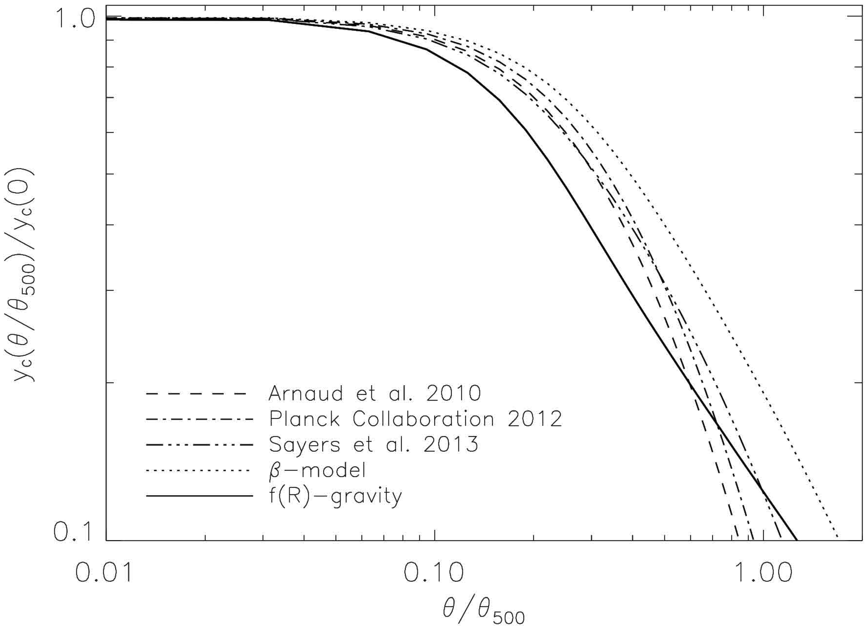
Clusters of galaxies are the largest virialized object in the Universe. They are the intermediate step between the galactic and the cosmological scales; thus, any relativistic theory of gravity must be capable of correctly describing their physics. Clusters typically contain a number of galaxies ranging from a few hundreds to one thousand, grouped in a region of ∼2 Mpc, contributing 3% to the total mass of the cluster. A more important component is represented by the baryons residing in a hot inter cluster (IC) gas. Although IC gas is highly rarefied, the electron number density is $n_e\sim {10}^{-4}-{10}^{-2}{\mathrm{cm}}^{-3}$; it makes up 12% of the total mass; and it reaches high temperatures ranging from ${10}^7$ to ${10}^8$ K, becoming a strong X-ray source with a luminosity typically ranging $L_X\sim {10}^{43}-{10}^{45}\mathrm{erg}/\mathrm{s}$.

One of the most promising tools to study clusters of galaxies is the Sunyaev–Zeldovich (SZ) effect [106,107]. CMB photons cross clusters of galaxies, and they are scattered off by free electrons present in the hot IC gas. This interaction produces secondary temperature fluctuations of the CMB power spectrum due to: (1) the thermal motion of the electrons in the gravitational potential well of the cluster (it is named Thermal Sunyaev-Zeldovich (TSZ) ; [106]); (2) the kinematic motion of the cluster as a whole with respect to the CMB rest frame (it is named Kinetic Sunyaev-Zeldovich KSZ ; [107]). In the direction of a cluster ($\stackrel{˰}{n}$), the SZ effect is given by:

$$\frac{T\left(\stackrel{˰}{n}\right)-T_0}{T_0}=\int \left[g\left(\nu \right)\frac{k_B{T}_e}{m_e{c}^2}+\frac{{\overrightarrow{v}}_{cl}\stackrel{˰}{n}}{c}\right]d\tau$$

(20)

where $d\tau ={\sigma }_T{n}_{e}dl$ is the optical depth, ${\sigma }_T$ is the Thomson cross-section, $k_B$ is the Boltzmann constant, $m_e{c}^2$ is the electron annihilation temperature, c is the speed of light, ν is the frequency of the observation and ${\overrightarrow{v}}_{cl}$ is the peculiar velocity of the cluster. $T_0=2.725\pm 0.002$ K [108] is the current CMB blackbody temperature, and $g\left(\nu \right)$ is the frequency dependence of the TSZ effect. In the non-relativistic limit, $g\left(x\right)=x\coth (x/2)-4$, with $x=h\nu /k_{B}T$ the reduced frequency. The physical description of the TSZ is commonly given by introducing the Comptonization parameter:

$$y_c=\frac{k_B{\sigma }_T}{m_e{c}^2}\int n_e\left(r\right)T_e\left(r\right)dl=\frac{{\sigma }_T}{m_e{c}^2}\int P_e\left(r\right)dl$$

(21)

where $P_e\left(r\right)$ is the electron pressure profile that must be specified to predict the TSZ anisotropies. Using X-ray observations and numerical simulations, several cluster profiles $\left(n_e{T}_e\right)$ have been proposed.

Isothermal β-model fits the X-ray emitting region of the clusters of galaxies well [109,110], with the electron density given by:

$$n_e\left(r\right)=n_{e,0}{\left[1+{\left(\frac{r}{r_c}\right)}^2\right]}^{-\frac{3\beta }{2}}$$

(22)

where $n_{e,0}$ is the central electron density and $r_c$ is the core radius. Those parameters, together with the electron temperature and the slope β, are determined from observations. Using the X-ray surface brightness of clusters, the slope value ranges in the interval $[0.6-0.8]$ [111].

The isothermal β-model over-predicts the TSZ effect in the outskirts of the cluster of galaxies [112]. Recently, a phenomenological parametrization of the electron pressure profile, derived from the numerical simulations, has been proposed [113,114]. The functional form of Universal pressure profile is:

$$p\left(x\right)\equiv \frac{P_0}{{\left(c_{500}x\right)}^{{\gamma }_a}{[1+{\left(c_{500}x\right)}^{{\alpha }_a}]}^{({\beta }_a-{\gamma }_a)/{\alpha }_a}}$$

(23)

where $x=r/r_{500}$, and $r_{500}$ is the radius at which the mean overdensity of the cluster is 500-times the critical density of the Universe at the same redshift. Then, $c_{500}$ is the concentration parameter at $r_{500}$. The model parameters were constrained using X-ray data [114,115] or CMB data [116]; their best fit values are quoted in Table 1.

Table 1. Parameters of universal pressure profile fitted by different groups using X-ray [114,115] and CMB data [116].

Model	$c_{\mathbf{500}}$	${\mathbf{\alpha }}_a$	${\mathbf{\beta }}_a$	${\mathbf{\gamma }}_a$	$P_{\mathbf{0}}$	Reference
Arnaud et al. 2010	1.177	1.051	5.4905	0.3081	8.403 $h_{70}^{3/2}$	[114]
Sayers et al. 2013	1.18	0.86	3.67	0.67	4.29	[115]
Planck et al. 2013	1.81	1.33	4.13	0.31	6.41	[116]

Table 1. Parameters of universal pressure profile fitted by different groups using X-ray [114,115] and CMB data [116].

Model	$c_{\mathbf{500}}$	${\mathbf{\alpha }}_a$	${\mathbf{\beta }}_a$	${\mathbf{\gamma }}_a$	$P_{\mathbf{0}}$	Reference
Arnaud et al. 2010	1.177	1.051	5.4905	0.3081	8.403 $h_{70}^{3/2}$	[114]
Sayers et al. 2013	1.18	0.86	3.67	0.67	4.29	[115]
Planck et al. 2013	1.81	1.33	4.13	0.31	6.41	[116]

Since TSZ does not depend on redshift in the ΛCDM model, clusters are a very important laboratory to test cosmology (see [117,118,119,120] and the references within), even to test the fundamental pillars of the Big Bang scenario [121,122].

In the last decade, SZ multi-frequency measurements have been reported by several groups: the Atacama Cosmology Telescope (ACT) [123,124,125,126], the South Pole Telescope (SPT) [127,128,129,130] and the Planck satellite [116,131,132,133]. Wilkinson Microwave Anisotropy Probe (WMAP) seven years [134] and Planck [116,131] data have discussed several apparent discrepancies with ΛCDM predictions. If these discrepancies are due to the physical complexity of clusters of galaxies or are due to the limitation of the theoretical modeling [135], it is an open question.

To study if these discrepancies are due to the theoretical modeling and, at the same time, to constrain/rule out ETGs at cluster scales, the pressure profile of a cluster of galaxies has been considered. On the one hand, it is interesting to study models that can explain the cluster without requiring any dark component [50]. On the other hand, models constructed to mimic the ΛCDM expansion history by replacing the DE with higher order terms in the gravitational Lagrangian must also describe the emergence of the LSS and the dynamical properties of clusters [51,52,53].

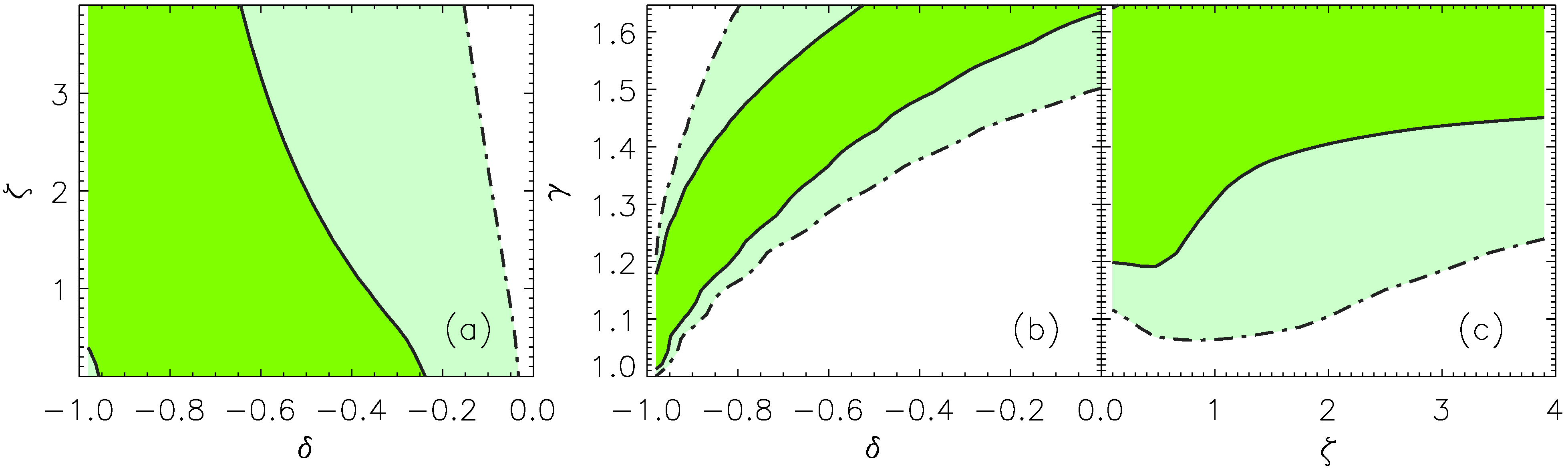
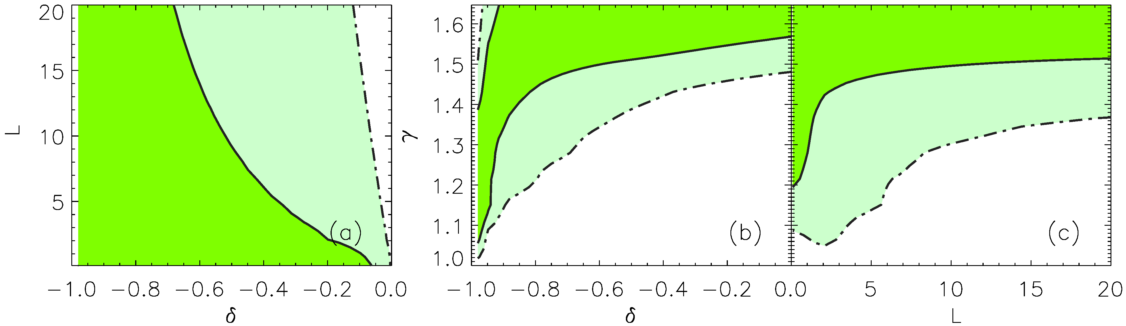
3.1. Pressure Profile from Yukawa-Like Gravitational Potential

One approach to test ETGs using the TSZ pressure profile is focused on the $f\left(R\right)$ Lagrangian that is expandable in Taylor’s series (Equation (13) in Section 2.2), where the Yukawa-like correction to the Newtonian potential, Equation (19), could be interpreted as the dynamical effect of DM in clusters of galaxies [50]. Making the hypothesis that: the gas is in hydrostatic equilibrium within the modified gravitational potential well (without any DM term):

$$\frac{dP\left(r\right)}{dr}=-\rho \left(r\right)\frac{d\text{Φ}\left(r\right)}{dr}$$

(24)

the gas follows a polytropic equation of state:

$$P\left(r\right)\propto {\rho }^{\gamma }\left(r\right)$$

(25)

the Equations (19), (24) and (25) can be numerically integrated to compute the pressure profiles by closing the system with the equation for the mass conservation:

$$\frac{dM\left(r\right)}{dr}=4\pi \rho \left(r\right)$$

(26)

Thus, the pressure profile will be a function of the two extra gravitational parameters $(\delta ,L)$ and the polytropic index γ. Let us remark that the density $\rho \left(r\right)$ includes only baryonic matter, without resorting to DM particles.

3.1.1. Data and Results

To constrain the model, the Planck (all Planck data are publicly available and can be downloaded from http://www.cosmos.esa.int/web/planck) 2013 data and an X-ray clusters catalog [136] have been used. In Figure 1, the predicted Comptonization parameter for the universal pressure profile with the parameters given in Table 1 and the $\beta =2/3$-model is compared with the $f\left(R\right)$-model with the parameters $[\delta ,L,\gamma ]=[-0.98,0.1,1.2]$. The model is particularized for the Coma cluster, located at redshift $z=0.023$, with core radius $r_c=0.25$ Mpc, X-ray temperature $T_X=6.48$ keV and electron density $n_{e,0}=3860{\mathrm{m}}^{-3}$. The plot shows that the higher order terms in the gravitational $f\left(R\right)$-Lagrangian could potentially explain the cluster without accounting for DM contribution.

The SZ emission was measured on the Spectral Matching Independent Component Analysis (SMICA) map (SMICA is a foreground-cleaned map; it has been constructed using a component separation method by combining the data at all frequencies [137]; the SMICA map has a $5^{\prime }$ resolution) at the locations of all X-ray selected clusters, and then, it was compared with the model prediction. The temperature anisotropies were averaged over rings of width ${\theta }_{500}/2$, where ${\theta }_{500}$ is the angular scale subtended by the $r_{500}$. The error associated with each data point was computed carrying out 1000 random simulations and evaluating the profile for each simulation. The analysis was performed by computing the likelihood function $logL=-{\chi }^2/2$ as:

$${\chi }^2\left(p\right)={\text{Σ}}_{i,j=0}^N(y(p,x_i)-d\left(x_i\right))C_{ij}^{-1}(y(p,x_j)-d\left(x_j\right))$$

(27)

where N is the number of data points, and $p=(\delta ,L,\gamma )$. In Equation (27), $d\left(x_i\right)$ are the data, and $C_{i,j}$ is the correlation matrix between the average temperature anisotropy on the discs and rings. Two parameterizations have been tested: (A) $L=\zeta r_{500}$, the scale length is different for each; clusters scale linearly with $r_{500}$; (B) L has the same value for all of the clusters. The models were constructing choosing “physical” flat priors on the parameters. Looking at the Yukawa-potential in Equation (19), if $\delta <-1$, it becomes repulsive, and if $\delta =-1$, it diverges; while the polytropic index γ was varied in the range corresponding to an isothermal and an adiabatic state of a monoatomic gas, respectively. The priors are summarized in Table 2.

Figure 1. Comptonization parameter for Comacluster (z = 0.023). The pressure profile is integrated along the line of sight for: the three universal profiles (dashed, solid and dash-dotted lines; the model parameters are quoted in Table 1); β = 2/3 model (long dashed line); and the f(R) model (red solid line, [δ, L, γ] = [-0.98, 0.1, 1.2]).

Figure 1. Comptonization parameter for Comacluster (z = 0.023). The pressure profile is integrated along the line of sight for: the three universal profiles (dashed, solid and dash-dotted lines; the model parameters are quoted in Table 1); β = 2/3 model (long dashed line); and the f(R) model (red solid line, [δ, L, γ] = [-0.98, 0.1, 1.2]).

Table 2. Priors on the parameters when modeling the cluster profile in $f\left(R\right)$-gravity.

Parameterization	δ	γ	L	ζ
(A)	$[-0.99,1.0]$	$[1.0,1.6]$	-	$[0.1,4]$
(B)	$[-0.99,1.0]$	$[1.0,1.6]$	$[0.1,20]$	-

Table 2. Priors on the parameters when modeling the cluster profile in $f\left(R\right)$-gravity.

Parameterization	δ	γ	L	ζ
(A)	$[-0.99,1.0]$	$[1.0,1.6]$	-	$[0.1,4]$
(B)	$[-0.99,1.0]$	$[1.0,1.6]$	$[0.1,20]$	-

Figure 2 and Figure 3 show the 2D contours at the $68\%$ and $95\%$ confidence levels of the marginalized likelihoods for both Parameterizations (A) and (B), respectively. Although the contours are opened and only upper limits can be obtained, the value $\delta =0$ is always excluded at more than the $95\%$ confidence level. Therefore, Newtonian potential without DM cannot fit cluster pressure profile, and thus, either DM or modified gravity must be the right description of the dynamical properties of the cluster of galaxies. The upper limits are summarized in Table 3.

Table 3. Upper limits on the model parameters for the cluster profile in $f\left(R\right)$-gravity.

	68% CL	95% CL	68% CL	95% CL
δ	< $-0.46$	< $-0.10$	< $-0.43$	< $-0.08$
γ	> $1.35$	> $1.12$	> $1.45$	> $1.2$
$L\left(or\zeta \right)$	< $2.5$	< $3.7$	< 12	< 19

Table 3. Upper limits on the model parameters for the cluster profile in $f\left(R\right)$-gravity.

	68% CL	95% CL	68% CL	95% CL
δ	< $-0.46$	< $-0.10$	< $-0.43$	< $-0.08$
γ	> $1.35$	> $1.12$	> $1.45$	> $1.2$
$L\left(or\zeta \right)$	< $2.5$	< $3.7$	< 12	< 19

Figure 2. 2D contours at the 68% (dark green) and 95% (light green) confidence levels of the marginalized likelihoods for Parameterization (A). In panel (a), (b), and (c) there are shown the 2D contours for the parameters (ζ, L), (δ, L), and (δ, ζ), respectively. Since the contours are opened, only upper limits on the parameters can be given.

Figure 2. 2D contours at the 68% (dark green) and 95% (light green) confidence levels of the marginalized likelihoods for Parameterization (A). In panel (a), (b), and (c) there are shown the 2D contours for the parameters (ζ, L), (δ, L), and (δ, ζ), respectively. Since the contours are opened, only upper limits on the parameters can be given.

Figure 3. 2D contours from the marginalized likelihoods for Parameterization (B). Contours follow the same convention of Figure 2. This parameterization also provides opened contours. Therefore, also in this case, one can only give upper limits on the parameters and can not distinguish which parameterization is the best one.

Figure 3. 2D contours from the marginalized likelihoods for Parameterization (B). Contours follow the same convention of Figure 2. This parameterization also provides opened contours. Therefore, also in this case, one can only give upper limits on the parameters and can not distinguish which parameterization is the best one.

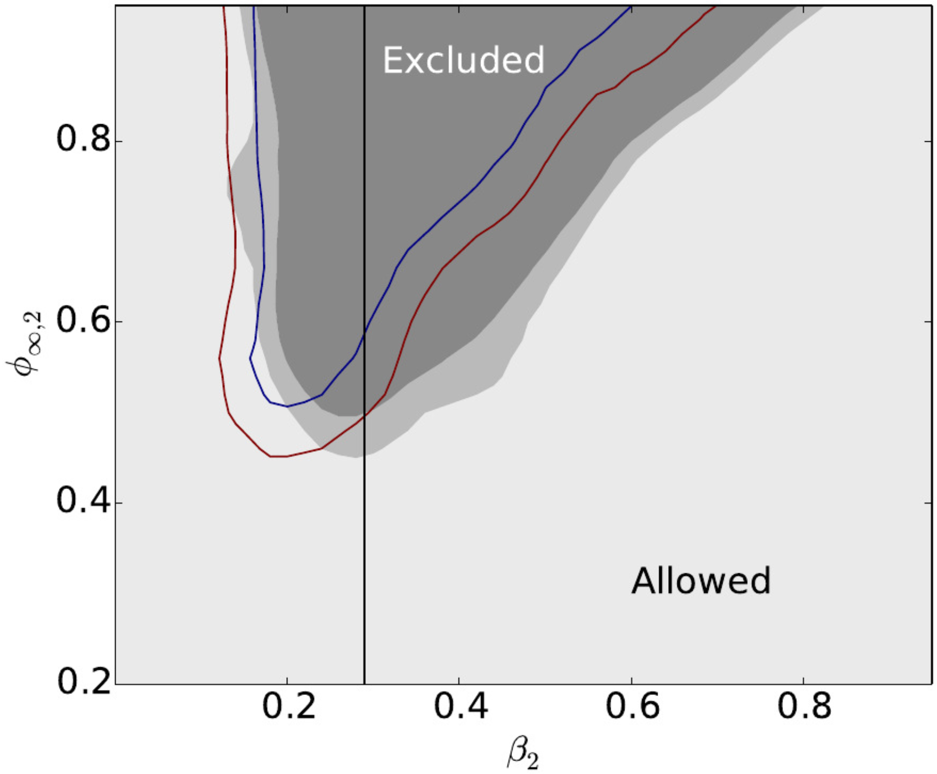
3.2. Chameleon Gravity: Hydrostatic and Weak Lensing Mass Profile of Galaxy Cluster

A second approach in using clusters of galaxies to test ETGs is focused on the chameleon gravity models that introduce a scalar field non-minimally coupled to the matter components. This coupling gives rise to the fifth force, which is tightly constrained at Solar System scales (see Section 2.1). The main difference with the other approach discussed above is that the chameleon gravity only eliminates DE, preserving the DM component as the source of the gravitational field needed to explain the emergence of the LSS.

Because of the screening mechanism, the effect of this force is negligible at small scales, and thus, it does not affect the density distribution of the IC gas in the cores of galaxy clusters, but its effect may not be totally screened in the outskirts. As a consequence, the gas distribution will be more compact in the outskirts under the effect of an additional pressure term that balances the effect of the fifth force. Thus, the hydrostatic mass of a cluster should be different from the mass obtained from weak gravitational lensing that depends only on the distribution of DM along the line of sight and does not assume hydrostatic equilibrium.

The model studied in [51,52] assumes the spherically-symmetric distribution of IC gas and DM. The IC gas is in hydrostatic equilibrium within the potential well generated by the DM distribution. Departures from hydrostatic equilibrium are parameterized, introducing a non-thermal term in the pressure, while the chameleon field directly contributes to the total amount of mass. The model is compared to lensing observations used to estimate the mass, with X-ray and SZ observations used to reconstruct the gas pressure profile [51,52,53].

Let us start writing down the equation of the hydrostatic equilibrium for the IC gas component:

$$\frac{1}{{\rho }_{\mathrm{gas}}\left(r\right)}\frac{d{P}_{\mathrm{tot}}\left(r\right)}{dr}=-\frac{GM(<r)}{r^2}$$

(28)

where $M_{}(<r)$ is the total mass enclosed in a sphere of radius r, ${\rho }_{\mathrm{gas}}$ is the gas density distribution within the sphere and $P_{\mathrm{tot}}$ is the total gas pressure that can be recast as:

$$P_{\mathrm{tot}}\left(r\right)=P_{\mathrm{th}}\left(r\right)+P_{\mathrm{non}-\mathrm{th}}\left(r\right)+P_{\varphi }\left(r\right)$$

(29)

including both thermal $\left(P_{\mathrm{th}}\left(r\right)\right)$ and non-thermal $\left(P_{\mathrm{non}-\mathrm{th}}\left(r\right)\right)$ pressure, and the term due to the chameleon field $\left(P_{\varphi }\left(r\right)\right)$. Thus, the total mass in Equation (28) is:

$$M_{}(<r)=M_{\mathrm{th}}\left(r\right)+M_{\mathrm{non}-\mathrm{th}}\left(r\right)+M_{\varphi }\left(r\right)$$

(30)

By definition, each term can be expressed as:

$$M_{\mathrm{th}}\left(r\right)\equiv -\frac{r^2}{G{\rho }_{\mathrm{gas}}\left(r\right)}\frac{d{P}_{\mathrm{th}}\left(r\right)}{dr}$$

(31)

$$M_{\mathrm{non}-\mathrm{th}}\left(r\right)\equiv -\frac{r^2}{G{\rho }_{\mathrm{gas}}\left(r\right)}\frac{d{P}_{\mathrm{non}-\mathrm{th}}\left(r\right)}{dr}$$

(32)

$$M_{\varphi }\left(r\right)\equiv -\frac{r^2}{G}\frac{\beta }{M_{\mathrm{Pl}}}\frac{d\varphi \left(r\right)}{dr}$$

(33)

$M_{\varphi }\left(r\right)$ is the mass associated with the chameleon field, and $M_{\mathrm{non}-\mathrm{th}}$ represents the departure from the hydrostatic equilibrium mass $M_{\mathrm{th}}$. Introducing the equation of state of the IC gas,

$$P_{\mathrm{th}}\left(r\right)=k{n}_{\mathrm{gas}}\left(r\right)T_{\mathrm{gas}}\left(r\right)$$

(34)

the Equation (31) can be re-written as

$$M_{\mathrm{th}}\left(r\right)=-\frac{k{T}_{\mathrm{gas}}\left(r\right)r}{\mu m_{\mathrm{p}}G}\left(\frac{dln{\rho }_{\mathrm{gas}}\left(r\right)}{dlnr}+\frac{dln{T}_{\mathrm{gas}}\left(r\right)}{dlnr}\right)$$

(35)

where the identity ${\rho }_{\mathrm{gas}}\left(r\right)=\mu m_{\mathrm{p}}{n}_{\mathrm{gas}}\left(r\right)$ has been considered with the mean molecular weight μ and the proton mass $m_{\mathrm{p}}$.

According to hydrodynamical simulations of the ΛCDM model [138,139], the non-thermal pressure term can be modeled as:

$$P_{\mathrm{non}-\mathrm{th}}\left(r\right)=\frac{g\left(r\right)}{1-g\left(r\right)}{n}_{\mathrm{gas}}\left(r\right)k{T}_{\mathrm{gas}}\left(r\right)$$

(36)

with:

$$g\left(r\right)={\alpha }_{\mathrm{nt}}{(1+z)}^{{\beta }_{\mathrm{nt}}}{\left(\frac{r}{r_{500}}\right)}^{n_{\mathrm{nt}}}{\left(\frac{M_{200}}{3\times {10}^{14}{M}_{\odot }}\right)}^{n_{\mathrm{M}}}$$

(37)

where ${\alpha }_{\mathrm{nt}}$, ${\beta }_{\mathrm{nt}}$, $n_{\mathrm{nt}}$ and $n_{\mathrm{M}}$ are constants. Therefore, the non-thermal mass term is:

$$M_{\mathrm{non}-\mathrm{thermal}}=-\frac{r^2}{G{\rho }_{\mathrm{gas}}^{\left(\mathrm{X}\right)}}\frac{d}{dr}\left(\frac{g}{1-g}{n}_{\mathrm{gas}}^{\left(\mathrm{X}\right)}k{T}_{gas}^{\left(\mathrm{X}\right)}\right)$$

(38)

This term is modeled without considering the chameleon field, and it has been shown to reproduce accurately the non-thermal contribution, even in $f\left(R\right)$-gravity. Nevertheless, a more accurate procedure would require modeling this term from hydrodynamical simulations under chameleon gravity. Finally, the total mass inferred from hydrostatic equilibrium has to be equal to the the total mass as inferred from weak lensing (WL):

$$M_{\mathrm{tot}}=M_{\mathrm{thermal}}+M_{\mathrm{non}-\mathrm{thermal}}+M_{\varphi }\equiv M_{\mathrm{WL}}$$

(39)

The DM density distribution is equally well described in the $f\left(R\right)$-model and in Newtonian gravity using the Navarro–Frenk–White (NFW) profile [140]. This profile has the following functional form [141]:

$$\rho \left(r\right)=\frac{{\rho }_{\mathrm{s}}}{r/r_{\mathrm{s}}{\left(1+r/r_{\mathrm{s}}\right)}^2}$$

(40)

and it has been constructed using N-body simulations of the ΛCDM model. Thus, the DM mass within the radius r is:

$$M_{\mathrm{DM}}(<r)=4\pi {\int }_0^{r}dr{r}^2\rho \left(r\right)=4\pi {\rho }_{\mathrm{s}}{r}_{\mathrm{s}}^3\left[ln(1+r/r_{\mathrm{s}})-\frac{r/r_{\mathrm{s}}}{1+r/r_{\mathrm{s}}}\right]\equiv M_{\mathrm{WL}}$$

(41)

that is equivalent to the WL mass if the DM component dominates over the baryonic one. The model has been tested using only COMA cluster [52] and using a sample of 58 X-ray selected cluster associated also with weak lensing measurements [53].

3.2.1. Data and Results

The chameleon model is essentially described by the following parameters $(\beta ,{\varphi }_{\infty })$ in Equations (5) and (7). In order to normalize them, those parameter have been replaced by:

$${\beta }_2=\frac{\beta }{1+\beta },$$

(42)

$${\varphi }_{\infty ,2}=1-e^{-\frac{{\varphi }_{\infty }}{{10}^{-4}{M}_{\mathrm{Pl}}}}$$

(43)

and constrained by carrying out the Monte Carlo Markov chain (MCMC) method using X-ray, SZ and WL observations. Another important parameter for studying clusters of galaxies is the critical radius:

$$r_{\mathrm{crit}}=\frac{\beta {\rho }_{\mathrm{s}}{r}_{\mathrm{s}}^3}{M_{\mathrm{Pl}}{\varphi }_{\infty }}-r_{\mathrm{s}}$$

(44)

where ${\rho }_{\mathrm{s}}$ is the density at this radius. It represents the distance from the DM halo center where the screening mechanism acts and it is not possible to distinguish between chameleon gravity and GR [51].

In [52], the authors have constrained chameleon gravity only using the Coma cluster ($z=0.0231$). For this cluster, they implement the MCMC method using the X-ray temperature profile reported by the X-ray Multi-Mirror Mission (XMM) -Newton [142] and Suzaku [143] for the inner and outer region, respectively. Then, the X-ray surface brightness profile was taken from XMM-Newton [144] and the SZ pressure profile measured by Planck [131]. For the WL counterpart, the measurements were reported in [145]. More recently, in [53], the authors have constrained the chameleon model using publicly-available weak lensing data provided by the Canada France Hawaii Lensing Survey (CFHTLenS; [146]), and X-ray data taken from the XMM-Newton archive. Their sample includes 58 clusters spanning the redshift range $z=[0.1-1.2]$, with measured X-ray temperatures $T_{\mathrm{x}}=[0.2-8]$ keV. For this sample of clusters, they also carried out an MCMC analysis. In Figure 4 are shown the two-dimensional contours for the parameters ${\beta }_2$ and ${\varphi }_{\infty ,2}$ as generated by [53]. The red and blue lines are the $95\%$ and $99\%$ confidence limits from [52]. Those results represent the best constraints on chameleon gravity using clusters. On the one hand, at low values of β, the departure from GR is too small to be detected with these observational errors. On the other hand, GR gravity is recovered within the critical radius $r_{\mathrm{crit}}$, and large values of β lead to a lower value for ${\varphi }_{\infty }$ that could keep $r_{\mathrm{crit}}$ in the whole cluster region. Although the analysis from [53] using the profiles outside of the critical radius of the cluster could better constrain large values of β, the analysis carried out by [52] also used SZ measurements and could discriminate better between GR and chameleon gravity at lower values of β. In both [52,53], it also constrained the term $f_{,\mathrm{R}0}$ from Equation (7). The result provides an upper limit today $|f_{,\mathrm{R}0}|<6\times {10}^{-5}$ at a $95\%$ of confidence level.

Figure 4. The confidence contours for the renormalized parameters (ϕ_∞,2, β₂) The 95% and 99% confidence levels are plotted in light gray and medium gray, respectively. The results are from [53]. The 95% and 99% confidence contours from [52] are over-plotted also in red and blue, respectively. The vertical line corresponds to |f,_R0| < 6 × 10⁻⁵.

Figure 4. The confidence contours for the renormalized parameters (ϕ_∞,2, β₂) The 95% and 99% confidence levels are plotted in light gray and medium gray, respectively. The results are from [53]. The 95% and 99% confidence contours from [52] are over-plotted also in red and blue, respectively. The vertical line corresponds to |f,_R0| < 6 × 10⁻⁵.

4. N-Body Hydrodynamical Simulations in f(R) Gravity

All chameleon-like theories of gravity need a specific screening mechanisms (Section 2.1). The effect of all such mechanisms is reflected on the non-linear perturbations of the matter distribution. Therefore, some of the most optimal tools to provide a full description of these mechanisms are modifications of standard N-body algorithms [147,148,149,150,151,152,153].

The aims were related to the study of the non-linear effects on the emergence of the LSS, such as the matter power spectrum [148,150,154], the redshift-space distortions [55] and the physical and statistical properties of the cold DM halos and voids [56,140,155,156,157,158,159,160]. However, the same scales and structures that could provide a powerful tool for testing the theory of gravitation are also seriously affected by non-linear astrophysical processes [161,162,163,164,165,166]. In the few last years, a very powerful code to investigate the combined effects of astrophysical processes and alternative theories of gravity has been developed [57]. The code is named Modified Gravity (MG)-GADGET. It was used to study the Hu–Sawicki model [103], pointing out the existence of an important degeneracy between modified gravity models and the uncertainties in the baryonic physics particularly, related to AGN feedback [57]. Afterwards, the code was combined with a massive neutrinos algorithm [167], to study the cosmic degeneracy between modified gravity and massive neutrinos. It was found that the deviations from the matter power spectrum in the ΛCDM model are, at most, of the order of 10% at $z=0$ taking $f\left(R\right)$ models with $f_{,R0}=-1\times {10}^{-4}$, and the total neutrinos mass ${\text{Σ}}_i{m}_{{\nu }_i}=0.4$ eV [168]. Using again the Hu–Sawicki parameterization, the effects of the model on the IC gas and its physical properties have been studied. It was found that the DM velocity dispersions in the $f\left(R\right)$ model are ∼$4/3$ larger than in ΛCDM, when low mass halos are considered. Nevertheless, the mass of the objects that are affected by the chameleon field depend on the value of the background field: for $|f_{,R0}|={10}^{-4}$ the field is never screened, nor for massive clusters; for $|f_{,R0}|={10}^{-5}$, the chameleon field is screened for mass above ∼${10}^{14.5}M\odot$; and for $|f_{,R0}|={10}^{-6}$, the Hu–Sawicki model does not produce any effect in the range of mass explored in [169]. Finally, MD-GADGET and the Hu–Sawicki model have been also used to study the synthetic Lyman-α absorption spectra using simulations that include star formation and cooling effects. The discrepancies with the simulations based on the ΛCDM model were at most $10\%$ with the background field fixed at $|f_{,R0}|={10}^{-4}$ [58].

All tests carried out using N-body simulations have provided several indications about the presence of a degeneracy between the effects of the complex baryonic physics (highly non-linear) and the effects of the modifications of the theory of gravitation. Even with the high accuracy of future data, without a full understanding of the non-linear astrophysical processes, it would be not possible to break the degeneracy and to constrain or rule out ETGs. Therefore, there is the need to fully explore this degeneracy with N-body simulations to know the level of bias introduced.

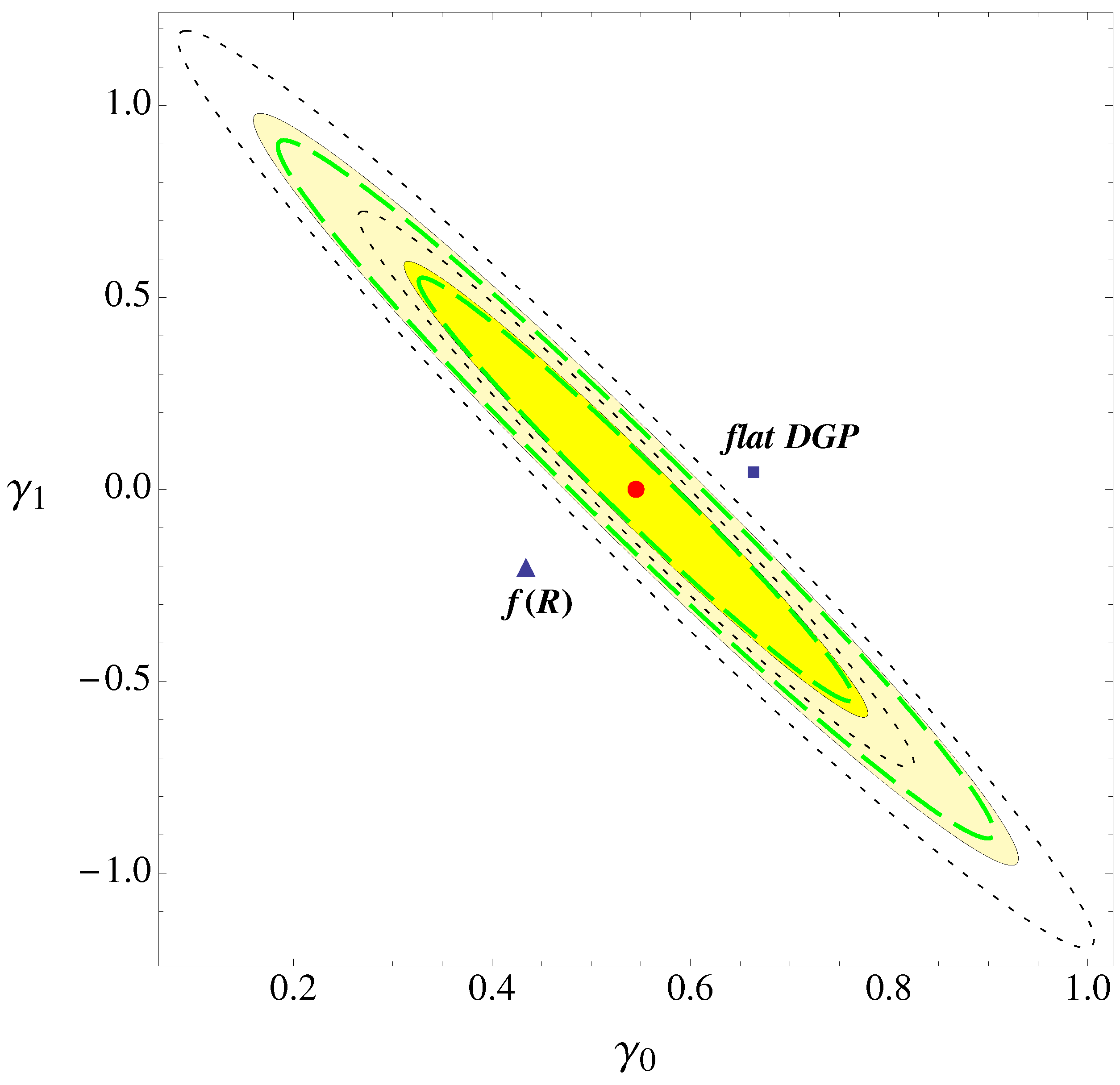
5. Constraining the Expansion History of the Universe in f(R) Gravity

Cosmological models can be tested looking at background evolution and also at the growth of the cosmic structures. Testing the $f\left(R\right)$ model at the background level allows finding the so-called “realistic” models that have the radiation, matter and DE eras very close to the ΛCDM ones. Although many realistic $f\left(R\right)$ models have been constructed, it should be considered that different models with a comparable late-time accelerated expansion and similar background densities’ evolution could differ in the growing of the matter density perturbations [170]. For example, it is well known that the effects at the background level of considering a collisional matter component filling the Universe are negligible. Nevertheless, non-collisional and collisional matter affect in different ways the evolution of matter perturbations, opening the possibility of distinguishing them [171]. Another problem is represented by the need to break the degeneracies between the evolving DE models and modified gravity in order to confirm/rule out models [172]. Thus, the growth factor (GF) data become extremely important to test modified gravity and to find their signatures. However, the available data have less accuracy than the other datasets, such as SNeIa, Baryonic Acoustic Oscillation (BAO) and $H\left(z\right)$; thus, it is not possible to fully constrain $f\left(R\right)$-models. This scenario will totally change with the forthcoming Euclid observations. That dataset will have an unprecedented accuracy, and it will allow constraining deviations from the standard model at a few percent level [54].

Let us start by the flat Friedman–Lemaitre–Robertson–Walker metric (FLRW),

$$d{s}^2=-d{t}^2+a^2\left(t\right)d{x}^2$$

(45)

where $a\left(t\right)$ is the rate expansion of the Universe. The Ricci scalar is related to the Hubble function, $H\equiv {\displaystyle \frac{\dot{a}\left(t\right)}{a\left(t\right)}}$ by the following expression:

$$R=6\left(2H^2+\dot{H}\right)$$

(46)

and using the non-relativistic matter and radiation approximation, the following conservation laws are satisfied:

$${\dot{\rho }}_m+3H{\rho }_m=0$$

(47)

$${\dot{\rho }}_{\gamma }+3H{\rho }_{\gamma }=0$$

(48)

Using Equations (2), (3), (45) and (46), the modified Friedman equations are obtained [173]:

$$3f_{,R}{H}^2={\kappa }^2({\rho }_m+{\rho }_{\gamma })+\frac{1}{2}(f_{,R}R-f\left(R\right))-3H{\dot{f}}_{,R}$$

(49)

$$-2f_{,R}\dot{H}={\kappa }^2({\rho }_m+\frac{4}{3}{\rho }_{\gamma })+{\ddot{f}}_{,R}-H{\dot{f}}_{,R}$$

(50)

To compute the the evolution of the matter density perturbations, ${\delta }_{\mathrm{m}}\equiv \frac{\delta {\rho }_{\mathrm{m}}}{{\rho }_{\mathrm{m}}}$, one can mainly follow two different approach:

• Sub-horizon approximation: The evolution of the matter density perturbations can be obtained solving the following equation [174]:

$${\ddot{\delta }}_{\mathrm{m}}+2H{\dot{\delta }}_{\mathrm{m}}-4\pi G_{\mathrm{eff}}(a,k){\rho }_{\mathrm{m}}{\delta }_{\mathrm{m}}=0$$

(51)

where k is the comoving wave number, and $G_{\mathrm{eff}}(a,k)$ is the effective gravitational constant. The explicit forms of $G_{eff}$ depend on the ETGs model. In the case of $f\left(R\right)$ gravity, it is given by [175]:

$$G_{\mathrm{eff}}(a,k)=\frac{G}{f_{,R}}\left[1+\frac{\left(k^2/a^2\right)\left(f_{,RR}/f_{,R}\right)}{1+3\left(k^2/a^2\right)\left(f_{,RR}/f_{,R}\right)}\right]$$

(52)

By definition, the growth factor $f_g$ is:

$$f_g\equiv \frac{dln{\delta }_{\mathrm{m}}}{dlna}$$

(53)

thus, Equation (51) becomes:

$$\frac{d{f}_g}{dlna}+f_g^2+\left(\frac{\dot{H}}{H}+2\right)f_g=\frac{3}{2}\frac{8\pi G_{\mathrm{eff}}{\rho }_{\mathrm{m}}}{3H^2}$$

(54)

Since Equation (51) does not give raise to analytical solutions, it is customary to introduce an efficient parameterization of the matter perturbations. The most common one is the so-called γ-parameterization:

$$f_g={\text{Ω}}_m^{\gamma }$$

(55)

$f_g^{\text{Λ}\mathrm{CDM}}$ is obtained for the value $\gamma \approx 0.545$. Therefore, any departures from this value could indicate the need to use a different model. More in general, the γ function could evolve with the redshift in the case of modified gravity models [176,178,179]:

$$\gamma \left(z\right)={\gamma }_0+{\gamma }_1\frac{z}{1+z}$$

(56)

This approach has been widely used to constrain the $f\left(R\right)$ gravity, pointing out that: the current data have not enough constraining power to discriminate between different modified gravity models and the ΛCDM model; the so-called growth index is the most efficient way to provide constraints on the model parameters; and the γ-parameterization represents the best way to measure deviation from the standard model [176,177].

• Dynamical variables: Starting from Equations (49) and (50), it is possible to reach a model-independent description of the evolution of the matter density perturbations [54,180,181]. Defining the following dimensionless variables:

$$x_1\equiv -\frac{{\dot{f}}_{,R}}{H{f}_{,R}}$$

(57)

$$x_2\equiv -\frac{f\left(R\right)}{6H^2{f}_{,R}}$$

(58)

$$x_3\equiv \frac{R}{6H^2}$$

(59)

$$x_4\equiv -\frac{{\kappa }^2{\rho }_{\gamma }}{3H^2{f}_{,R}}$$

(60)

the density parameters and the effective equation of state of the system can be written as:

$${\text{Ω}}_{\gamma }\equiv x_4$$

(61)

$${\text{Ω}}_m\equiv \frac{{\kappa }^2{\rho }_m}{3H^2{f}_{,R}}=1-x_1-x_2-x_3-x_4$$

(62)

$${\text{Ω}}_X\equiv x_1+x_2+x_3$$

(63)

$$w_{eff}\equiv -\frac{1}{3}(2x_3-1)$$

(64)

The background evolution is given by:

$$x_1^{\prime }=-1-x_3-3x_2+x_1^2-x_1{x}_3+x_4$$

(65)

$$x_2^{\prime }={\displaystyle \frac{x_1{x}_3}{m}}-x_2(2x_3-4-x_1)$$

(66)

$$x_3^{\prime }=-{\displaystyle \frac{x_1{x}_3}{m}}-2x_3(x_3-2)$$

(67)

$$x_4^{\prime }=-2x_3{x}_4-x_1{x}_4$$

(68)

where the prime indicates the derivative with respect to the scale factor $d/dlna$, and m is a parameter related to the theory that indicates how much a specific model is close to the ΛCDM (or how much it deviates from it). This parameter is defined as:

$$m\equiv {\displaystyle \frac{dln{f}_{,R}}{dlnR}}={\displaystyle \frac{R{f}_{,RR}}{f_{,R}}}$$

(69)

and by definition, one also finds the following identity:

$$r\equiv -{\displaystyle \frac{dlnf}{dlnR}}=-{\displaystyle \frac{R{f}_{,R}}{f}}={\displaystyle \frac{x_3}{x_2}}$$

(70)

Equations (65) to (70) represent a closed system that can be integrated numerically, obtaining the evolution of the background densities perturbations. We just need to choose an $f\left(R\right)$-model to compute the two parameters m and r that we need to integrate the system. From the analysis of the critical points, we have several conditions that an $f\left(R\right)$ model has to respect to be cosmologically viable [54,180]. In general, only models with $m\ge 0$ and very close to the ΛCDM model ($f\left(R\right)=R-2\text{Λ}$) are cosmologically viable. Thus, the equations for the matter density perturbations are [181,182]:

$$\begin{array}{cc}\hfill {\delta }_m^{\prime \prime }& +\left(x_3-\frac{1}{2}{x}_1\right){\delta }_m^{\prime }-\frac{3}{2}(1-x_1-x_2-x_3){\delta }_m\hfill \\ & =\frac{1}{2}[\left\{\frac{k^2}{x_5^2}-6+3x_1^2-3x_1^{\prime }-3x_1(x_3-1)\right\}\delta \widetilde{f_{,R}}\hfill \\ & +3(-2x_1+x_3-1)\delta {\widetilde{f_{,R}}}^{\prime }+3\delta {\widetilde{f_{,R}}}^{\prime \prime }]\hfill \end{array}$$

(71)

$$\begin{array}{cc}\hfill \delta {\widetilde{f_{,R}}}^{\prime \prime }& +(1-2x_1+x_3)\delta {\widetilde{f_{,R}}}^{\prime }\hfill \\ & +\left[\frac{k^2}{x_5^2}-2x_3+\frac{2x_3}{m}-x_1(x_3+1)-x_1^{\prime }+x_1^2\right]\delta \widetilde{f_{,R}}\hfill \\ & =(1-x_1-x_2-x_3){\delta }_m-x_1{\delta }_m^{\prime }\hfill \end{array}$$

(72)

where $\delta \widetilde{f_{,R}}\equiv \delta f_{,R}/f_{,R}$ and $x_5\equiv aH$ satisfies:

$$x_5^{\prime }=(x_3-1)x_5.$$

(73)

The evolution at all scales of the growth of the matter density perturbation, ${\delta }_m$, could be obtained via numerical integration. However, a more straightforward approach is to assume that the growth rate, $f_g$, is a function of time, but not of scale [183,184,185,186,187], and to use the γ-parameterization in Equations (55) and (56).

The detection of possible deviation from ΛCDM model has been studied fitting the γ-parameterization to the forthcoming Euclid dataset [54]. Assuming the ΛCDM model as the reference model, it has been found that: the forthcoming data will be able to constrain the parameter γ and w with an accuracy of 4% and 2% if they do not depend on redshift (standard evolution) and to clearly distinguish the ΛCDM from alternative scenarios at more than $2\sigma$; see Figure 5.

Figure 5. The 1σ and 2σ marginalized contours for the parameters γ₀ and γ₁ in the γ-parameterization. Shown is the reference case (shaded yellow regions), with the optimistic error bars (green long-dashed ellipses) and the pessimistic ones (black dotted ellipses). Red circle represent the ΛCDM model (γ = 0.545), while triangles represent the f(R) model [54].

Figure 5. The 1σ and 2σ marginalized contours for the parameters γ₀ and γ₁ in the γ-parameterization. Shown is the reference case (shaded yellow regions), with the optimistic error bars (green long-dashed ellipses) and the pessimistic ones (black dotted ellipses). Red circle represent the ΛCDM model (γ = 0.545), while triangles represent the f(R) model [54].

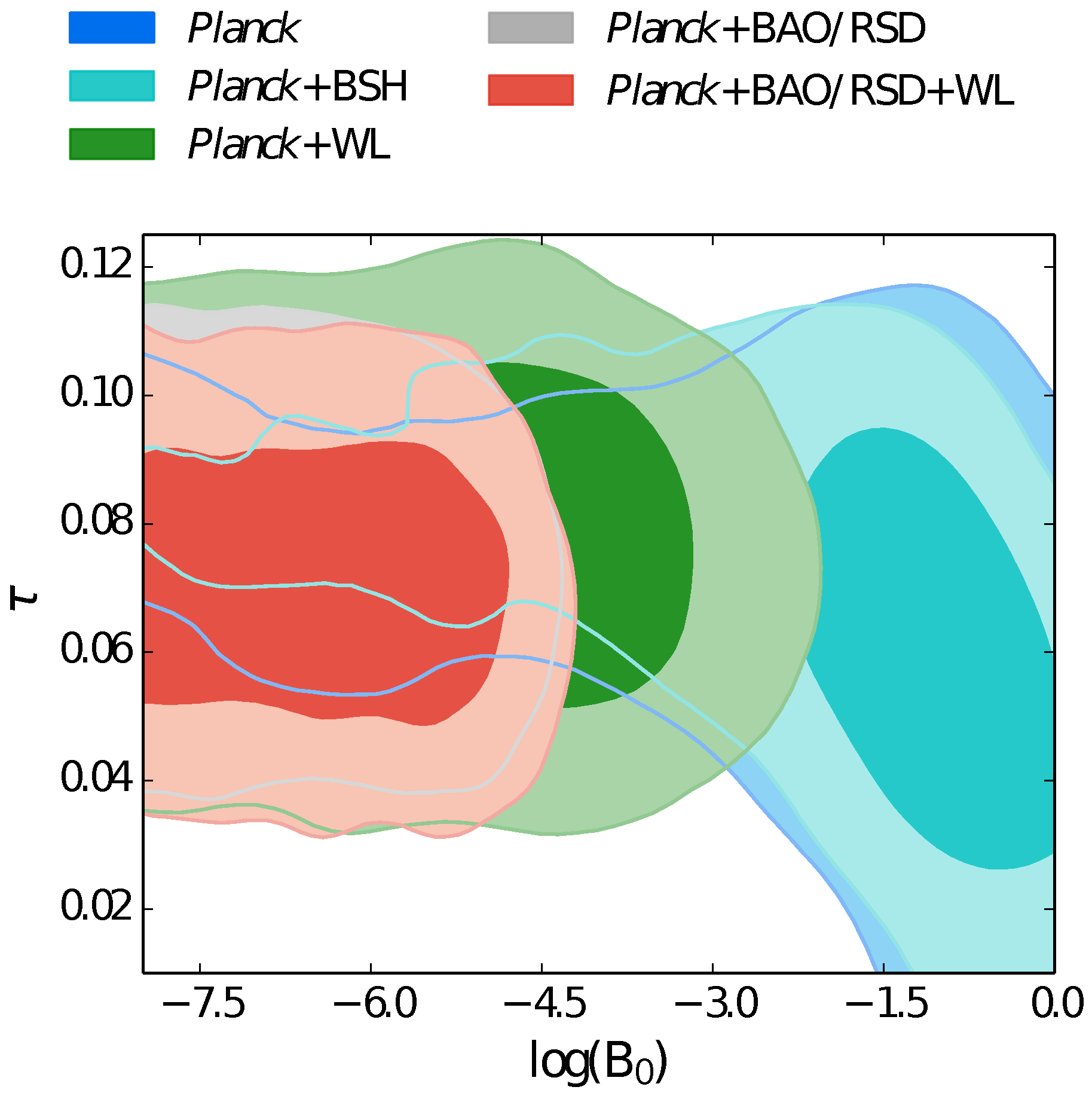
6. Testing Gravity Using the Cosmic Microwave Background Data

The CMB temperature anisotropies play a key rule to constrain the cosmological model. They are mostly generated at the last-scattering surface, and thus, they provide a way to probe the early Universe [13,17,133]. However, the lack of a full-consistent theoretical framework and the fine tuning problem related to the cosmological constant, Λ, have encouraged studying wide classes of alternative DE or modified gravity models. The most difficult challenge of modern cosmology is to use current and forthcoming datasets to discriminate between those alternative visions of the Universe [54,188,189,190,191]. Many of those models mimic the ΛCDM at background evolution, but differ in the perturbations, and they could produce several effects on the CMB power spectrum. As an example, different models could have different expansion histories that shift the location of the peaks [192], and could affect the gravitational potential at late time, changing the integrated Sachs–Wolfe (ISW) effect [193,194]. Moreover, modification of the gravitational theory should be reflected in modifications of the lensing potential [195,196], the growth of the structures [197,198,199,200] and also the amplitude of the primordial B-modes [201,202].

Modified gravity models affect the evolution of the Universe at both the background and the perturbation [203,204,205,206]. There are mainly two different approaches used to constrain alternative models of gravity: the parametrized modified gravity approach and the effective field theory.

The parametrized modified gravity approach constructs functions probing the geometry of space-time and the growth of perturbations. Starting from a spatially-flat FLRW metric, the perturbed line element in the Newtonian gauge is given by:

$$d{s}^2=a{\left(\tau \right)}^2[-(1+2\text{Ψ})d{\tau }^2+(1-2\text{Φ})d{x}^2]$$

(74)

where τ is the conformal time. Ψ and Φ are the two scalar gravitational potentials that are a function of the scale $\text{Ψ}=\text{Ψ}(k,a)$ and $\text{Φ}=\text{Φ}(k,a)$ and are related to the energy-momentum tensor, $T_{\mu \nu }$, through Einstein’s equations. Those potentials can be modeled to fix all degrees of freedom in order to match observational data. Moreover, the difference of those two potentials $\text{Φ}-\text{Ψ}$, which is the anisotropic stress, has to be equal to zero in GR. Any departure from this value would indicate a departure from GR [207,208]. One of the most common parameterization is implemented in the Modification of Growth with Code for Anisotropies in the Microwave Background (the code is publicly available at http://www.sfu.ca/ aha25/MGCAMB.html) (MGCAMB) [209,210], and it considers the following:

$$k^2\text{Ψ}=-4\pi G{a}^2\mu (k,a)\rho \Delta$$

(75)

$$\frac{\text{Φ}}{\text{Ψ}}=\gamma (k,a)$$

(76)

to parameterize the Poisson and the anisotropic stress equations using two scale and time-dependent functions $\mu (k,a)$ and $\gamma (k,a)$. Those two functions are determined by choosing the particular model. For example, some classes of $f\left(R\right)$ models lead to [211]:

$$\mu (k,a)=\frac{1+{\beta }_1{\lambda }_1^2{k}^2{a}^s}{1+{\lambda }_1^2{k}^2{a}^s}$$

(77)

$$\gamma (k,a)=\frac{1+{\beta }_2{\lambda }_2^2{k}^2{a}^s}{1+{\lambda }_2^2{k}^2{a}^s}$$

(78)

where the parameters ${\beta }_i$ are dimensionless and represent the couplings, and the parameters ${\lambda }_i$ are lengths. Those functional forms have been used in early studies to forecast errors of the parameters for the Dark Energy Survey (www.darkenergysurvey.org/) (DES, [212]) and Large Synoptic Survey Telescope (http://www.lsst.org/lsst/) (LSST, [213]) surveys [210]. The main limitation of this approach is the use of the quasi-static regime assuming that the scales at which one is interested are still linear and smaller than the horizon. Furthermore, the time derivatives are neglected.

Effective field theory (EFT) [214,215] describes the whole range of the scalar field theories. The Lagrangian preserves the isotropy and homogeneity of the Universe at the background, providing a more general approach without assuming the quasi-static regime, but adding much more free parameters that must be constrained. The $f\left(R\right)$-models are a sub-class of those theories. The action of EFT reads:

$$\begin{array}{ccc}\hfill S& =& \int d^{4}x\sqrt{-g}\left\{\frac{m_0^2}{2}\left[1+\text{Ω}\left(\tau \right)\right]R+\text{Λ}\left(\tau \right)-a^{2}c\left(\tau \right)\delta g^{00}\right.\hfill \\ & & +\frac{M_2^4\left(\tau \right)}{2}{\left(a^2\delta g^{00}\right)}^2-{\overline{M}}_1^3\left(\tau \right)2a^2\delta g^{00}\delta K_{\mu }^{\mu }\hfill \\ & & -\frac{{\overline{M}}_2^2\left(\tau \right)}{2}{\left(\delta K_{\mu }^{\mu }\right)}^2-\frac{{\overline{M}}_3^2\left(\tau \right)}{2}\delta K_{\nu }^{\mu }\delta K_{\mu }^{\nu }+\frac{a^2{\stackrel{˰}{M}}^2\left(\tau \right)}{2}\delta g^{00}\delta R^{\left(3\right)}\hfill \\ & & \left.+m_2^2\left(\tau \right)\left(g^{\mu \nu }+n^{\mu }{n}^{\nu }\right){\partial }_{\mu }\left(a^2{g}^{00}\right){\partial }_{\nu }\left(a^2{g}^{00}\right)\phantom{\frac{m_0^2}{2}}\right\}\hfill \\ & & +S_{\mathrm{m}}\left[{\chi }_i,g_{\mu \nu }\right]\hfill \end{array}$$

(79)

where $\delta R^{\left(3\right)}$ is its spatial perturbation, $K_{\nu }^{\mu }$ is the extrinsic curvature, $m_0$ is the bare (reduced) Planck mass and $S_{\mathrm{m}}$ is the matter part of the action, including all fluid components, such as baryons, cold DM, radiation, and neutrinos, but it does not include DE. The nine time-dependent functions [216] $\{\text{Ω},c,\text{Λ},{\overline{M}}_1^3,{\overline{M}}_2^4,{\overline{M}}_3^2,M_2^4,{\stackrel{˰}{M}}^2,m_2^2\}$, have to be fixed to specify the theory. The EFT has been implemented in the publicly-available EFTCAMBcode (http://www.lorentz.leidenuniv.nl/h̃u/codes/, Version 1.1, October 2014.) [59,217], that numerically solves both the background and perturbation equations. The code has been used to constrain massive neutrinos in $f\left(R\right)$ gravity [59].

Planck collaboration has used in both approaches to fit $f\left(R\right)$ models to investigate their effect combining early time datasets, such as CMB, and cosmological datasets at much lower redshift [14]. In general, $f\left(R\right)$ models require setting the initial condition:

$${\displaystyle \underset{R\to \infty }{lim}}\frac{f\left(R\right)}{R}=0$$

(80)

and the boundary condition:

$$B\left(z\right)=\frac{f_{RR}}{1+f_R}\frac{H\dot{R}}{\dot{H}-H^2}$$

(81)

High values of $B_0$, its present value, change the ISW effect and the CMB lensing potential [211,218,219], Marchini2013. Their analysis has shown the presence of a degeneracy between the optical depth τ and $B_0$ that can be broken adding other probes on the structure formation, such as weak lensing, CMB lensing or redshift-space distortions (see Figure 6).

The same study carried out using MGCAMB code led to the same results within the uncertainties, improving the previous constraint on $B_0$ [220].

Nevertheless, both EFTCAMB and MGCAMB assume a specific background cosmology. MGCAMB code assumes for the background evolution the ΛCDM or wCDM, while EFTCAMB assumes a fixed background evolution, and the CMB power spectrum is calculated for an $f\left(R\right)$ model re-constructed by the fixed expansion history. A more recent code, named $f\left(R\right)$ Code for Anisotropies in the Microwave Background (FRCAMB) [221], allows reconstructing the CMB power spectrum for any $f\left(R\right)$ model by specifying the first and second derivatives of the Lagrangian. Although the results obtained are consistent with the one from EFTCAMB and MGCAMB, the code has the advantage of being designed for any $f\left(R\right)$ model at both the background and perturbation level.

Figure 6. The $68\%$ and $95\%$ contour plots for the two parameters, $\{{\mathrm{Log}}_{10}\left({\mathrm{B}}_0\right),\tau \}$. There is a degeneracy between the two parameters for Planck temperature power spectrum (TT) + BSH (the combination of BAO, SNIa, and $H_0$ datasets). Adding lensing will break the degeneracy between the two. Here, Planck indicates Planck TT.

Figure 6. The $68\%$ and $95\%$ contour plots for the two parameters, $\{{\mathrm{Log}}_{10}\left({\mathrm{B}}_0\right),\tau \}$. There is a degeneracy between the two parameters for Planck temperature power spectrum (TT) + BSH (the combination of BAO, SNIa, and $H_0$ datasets). Adding lensing will break the degeneracy between the two. Here, Planck indicates Planck TT.

7. Discussion and Future Perspectives

In this review, we have outlined the possibilities offered by the current and the forthcoming astrophysical and cosmological dataset to constrain or rule out the $f\left(R\right)$-models. It is mandatory to search for the answer to one of the fundamental questions in modern cosmology: is GR the effective theory of gravitation? This question comes from the evidence that GR is not enough to fully explain the cosmological evolution of the Universe and the emergence of the clustered structures, and it needs the addition of two unknown components. The difficulties in identifying the DM and DE components at a fundamental level have opened the possibility that the answer resides in modifying the theory of gravity. Nevertheless, having an alternative demands testing it study the physical phenomena at much smaller scales than the cosmological ones. To this effect, much analysis has been carried out to ensure that modified gravity could recover the tight constraints at the Solar System scale. Models that survive these probes have been used to test galactic and extragalactic scales. Clusters of galaxies provide an excellent laboratory to probe the different features of the different modified gravity models. The variety of the phenomenology related to the cluster physics allows one to use SZ, X-ray and WL observations in order to constrain $f\left(R\right)$-models. Many efforts have been also devoted to quantitatively describing the physical effects of alternative cosmological scenarios. Those efforts have required developing new algorithms for hydrodynamical N-body simulations, to study the degeneracy between baryonic physics and modifications of gravity and also new Boltzmann codes to predict the CMB power spectrum and to take advantage of the Planck data to constrain modified gravity models.

Nevertheless, a self-consistent picture has not been reached yet. The current datasets do not have enough statistical power to discriminate between modified gravity models and standard cosmology, and when the needed precision is present, several degeneracies have been found. Next generation experiments, such as the LSST [213] and the Wide-Field Infrared Survey Telescope (WFIRST) (http://wfirst.gsfc.nasa.gov/) [222], will undertake large imaging surveys of the sky, while other surveys, such as Euclid [223] and the Big-Baryon Oscillation Spectroscopic Survey (BigBOSS) [224], will make spectroscopic measurements of galaxies. The combination of all forthcoming datasets will hopefully put strong constraints on the evolution of the Universe and the emergence of the LSS, allowing us to discriminate between the concordance ΛCDM model and its alternatives.

References

1. Perlmutter, S.; Gabi, S.; Goldhaber, G.; Goobar, A.; Groom, D.E.; Hook, I.M.; Kim, A.G.; Kim, M.Y.; Lee, J.C.; Pain, R.; et al. Measurements of the Cosmological Parameters Omega and Lambda from the First Seven Supernovae at z ≥ 0.35. Astrophys. J. 1997, 483, 565. [Google Scholar]
2. Riess, A.G.; Strolger, L.-G.; Tonry, J.; Casertano, S.; Ferguson, H.C.; Mobasher, B.; Challis, P.; Filippenko, A.V.; Jha, S.; Li, W.; et al. Type Ia Supernova Discoveries at z > 1 from the Hubble Space Telescope: Evidence for Past Deceleration and Constraints on Dark Energy Evolution. Astrophys. J. 2004, 607, 665–687. [Google Scholar] [CrossRef]
3. Astier, P.; Guy, J.; Regnault, N.; Pain, R.; Aubourg, E.; Balam, D.; Basa, S.; Carlberg, R.G.; Fabbro, S.; Fouchez, D.; et al. The Supernova Legacy Survey: Measurement of ΩM, ΩΛ and w from the first year data set. Astron. Astrophys. 2006, 447, 31–48. [Google Scholar] [CrossRef]
4. Suzuki, N.; Rubin, D.; Lidman, C.; Aldering, G.; Amanullah, R.; Barbary, K.; Barrientos, L.F.; Botyanszki, J.; Brodwin, M.; Connolly, N.; et al. The Hubble Space Telescope Cluster Supernova Survey. V. Improving the Dark-energy Constraints above z > 1 and Building an Early-type-hosted Supernova Sample. Astrophys. J. 2012, 746, 85. [Google Scholar]
5. Pope, A.C.; Matsubara, T.; Szalay, A.S.; Blanton, M.R.; Eisenstein, D.J.; Gray, J.; Jain, B.; Bahcall, N.A.; Brinkmann, J.; Budavari, T.; et al. Cosmological Parameters from Eigenmode Analysis of Sloan Digital Sky Survey Galaxy Redshifts. Astrophys. J. 2004, 607, 655. [Google Scholar] [CrossRef]
6. Percival, W.J.; Baugh, C.M.; Bland-Hawthorn, J.; Bridges, T.; Cannon, R.; Cole, S.; Colless, M.; Collins, C.; Couch, W.; Dalton, G.; et al. The 2dF Galaxy Redshift Survey: The power spectrum and the matter content of the Universe. Mon. Not. R. Astron. Soc. 2001, 327, 1297–1306. [Google Scholar] [CrossRef]
7. Tegmark, M.; Blanton, M.R.; Strauss, M.A.; Hoyle, F.; Schlegel, D.; Scoccimarro, R.; Vogeley, M.S.; Weinberg, D.H.; Zehavi, I.; Berlind, A.; et al. The Three-Dimensional Power Spectrum of Galaxies from the Sloan Digital Sky Survey. Astrophys. J. 2004, 606, 702. [Google Scholar] [CrossRef]
8. Hinshaw, G.; Larson, D.; Komatsu, E.; Spergel, D.N.; Bennett, C.L.; Dunkley, J.; Nolta, M.R.; Halpern, M.; Hill, R.S.; Odegard, N.; et al. Nine-Year Wilkinson Microwave Anisotropy Probe (WMAP) Observations: Cosmological Parameter Results. Astrophys. J. Suppl. Ser. 2013, 208, 19. [Google Scholar] [CrossRef]
9. Planck Collaboration. Planck 2013 Results. XV. CMB power spectra and likelihood. Astron. Astrophys. 2013, 571, A15. [Google Scholar]
10. Planck Collaboration. Planck 2013 Results. XX. Cosmology from Sunyaev? Zeldovich cluster counts. Astron. Astrophys. 2013, 571, A20. [Google Scholar]
11. Planck Collaboration. Planck 2013 Results. XXIII: Isotropy and statistics of the CMB. Astron. Astrophys. 2013, 571, A23. [Google Scholar]
12. Planck Collaboration. Planck Results. I. Overview of products and scientific results. 5 February 2015; arXiv:1502.01582v1. [Google Scholar]
13. Planck Collaboration. Planck Results. XIII. Cosmological parameters. 6 February 2015; arXiv:1502.01589v1. [Google Scholar]
14. Planck Collaboration. Planck Results. XIV. Dark energy and modified gravity. 5 February 2015; arXiv:1502.01590v1. [Google Scholar]
15. Planck Collaboration. Planck Results. XVII. Primordial non-Gaussianity. 5 February 2015; arXiv:1502.01592v1. [Google Scholar]
16. Planck Collaboration. Planck Results. XVIII. Background geometry and topology of the Universe. 5 February 2015; arXiv:1502.01593v1. [Google Scholar]
17. Planck Collaboration. PPlanck 2015 results. XX. Constraints on inflation. 7 February 2015; arXiv:1502.02114v1. [Google Scholar]
18. Planck Collaboration. Planck Results. XXI. The integrated Sachs-Wolfe effect. 5 February 2015; arXiv:1502.01595v1. [Google Scholar]
19. Blake, C.; Kazin, E.A.; Beutler, F.; Davis, T.M.; Parkinson, D.; Brough, S.; Colless, M.; Contreras, C.; Couch, W.; Croom, S.; et al. The WiggleZ Dark Energy Survey: Mapping the distance-redshift relation with baryon acoustic oscillations. Mon. Not. R. Astron. Soc. 2011, 418, 1707–1724. [Google Scholar] [CrossRef]
20. Capozziello, S.; De Laurentis, M. Extended theories of gravity. Phys. Rep. 2011, 509, 167–321. [Google Scholar] [CrossRef]
21. Nojiri, S; Odintsov, S.D. Unified cosmic history in modified gravity: from F(R) theory to Lorentz non- invariant models. Phys. Rept. 2011, 505, 59–144. [Google Scholar]
22. Capozziello, S.; Francaviglia, M. Extended theories of gravity and their cosmological and astrophysical applications. Gen. Relativ. Gravit. 2008, 40, 357–420. [Google Scholar] [CrossRef]
23. Capozziello, S.; De Laurentis, M.; Faraoni, V. A Bird’s eye view of f(R)-gravity. 2 October 2009; arXiv:0909.4672v2 [gr-qc]. [Google Scholar]
24. Olmo, G.J. Palatini Approach to Modified Gravity: f(R) Theories and Beyond. Int. J. Mod. Phys. D 2011, 20, 413–462. [Google Scholar] [CrossRef]
25. Lobo, F.S.N. The Dark side of gravity: Modified theories of gravity. 10 July 2008; arXiv:0807.1640 [gr-qc]. [Google Scholar]
26. De Felice, A.; Tsujikawa, S. f(R) Theories. Available online: http://www.emis.ams.org/journals/ LRG/Articles/lrr-2010-3/download/lrr-2010-3Color.pdf (accessed on 22 July 2015).
27. Sotiriou, T.; Faraoni, V. f(R) Theories Of Gravity. Rev. Mod. Phys. 2010, 82, 451. [Google Scholar] [CrossRef]
28. Capozziello, S.; De Laurentis, M. F(R) theories of gravitation. Scholarpedia 2015, 10, 31422. [Google Scholar] [CrossRef]
29. Capozziello, S.; De Laurentis, M.; Odintsov, S.D.; Stabile, A. Hydrostatic equilibrium and stellar structure in f(R) gravity. Phys. Rev. D 2012, 83, 064004. [Google Scholar] [CrossRef]
30. Capozziello, S.; De Laurentis, M.; de Martino, I.; Formisano, M.; Odintsov, S.D. Jeans analysis of self-gravitating systems in f(R) gravity. Phys. Rev. D 2012, 85, 044022. [Google Scholar] [CrossRef]
31. Arbuzova, E.V.; Dolgov, A.D.; Reverberi, L. Jeans instability in classical and modified gravity. Phys. Lett. B 2014, 739, 279–284. [Google Scholar] [CrossRef]
32. Farinelli, R.; De Laurentis, M.; Capozziello, S.; Odintsov, S.D. Numerical solutions of the modified Lane-Emden equation in f(R)-gravity. Mon. Not. R. Astron. Soc. 2014, 440, 2909–2915. [Google Scholar] [CrossRef]
33. Astashenok, A.V.; Capozziello, S.; Odintsov, S.D. Magnetic neutron stars in f(R) gravity. Astrophys. Space Sci. 2015, 355, 333–341. [Google Scholar] [CrossRef]
34. Astashenok, A.V.; Capozziello, S.; Odintsov, S.D. Extreme neutron stars from Extended Theories of Gravity. J. Cosmol. Astropart. Phys. 2015. [Google Scholar] [CrossRef] [PubMed]
35. De Laurentis, M.; de Martino, I. Testing f(R)-theories using the first time derivative of the orbital period of the binary pulsars. Mon. Not. R. Astron. Soc. 2013, 431, 741–748. [Google Scholar] [CrossRef]
36. De Laurentis, M.; de Martino, I. Probing the physical and mathematical structure of f(R) gravity by PSR J0348 + 0432. Int. J. Geom. Methods Mod. Phys. 2015, 12, 1550040. [Google Scholar]
37. De Laurentis, M.; Capozziello, S. Quadrupolar gravitational radiation as a test-bed for f(R)-gravity. Astropart. Phys. 2011, 35, 257–265. [Google Scholar] [CrossRef]
38. De Laurentis, M.; de Rosa, R.; Garufi, F; Milano, L. Testing gravitational theories using eccentric eclipsing detached binaries. Mon. Not. R. Astron. Soc. 2012, 424, 2371–2379. [Google Scholar]
39. Bogdanos, C.; Capozziello, S.; De Laurentis, M.; Nesseris, S. Massive, massless and ghost modes of gravitational waves from higher-order gravity. Astropart. Phys. 2010, 34, 236–244. [Google Scholar] [CrossRef]
40. Antoniadis, J.; Freire, P.C.C.; Wex, N.; Tauris, T.M.; Lynch, R.S.; van Kerkwijk, M.H.; Kramer, M.; Bassa, C.; Dhillon, V.S.; Driebe, T.; et al. A Massive Pulsar in a Compact Relativistic Binary. Science 2013. [Google Scholar] [CrossRef] [PubMed]
41. Clifton, T.; Barrow, J.D. Observational Constraints on the Completeness of Space near Astrophysical Objects. Phys. Rev. D 2010, 81, 063006. [Google Scholar] [CrossRef]
42. Clifton, T.; Barrow, J.D. The Power of General Relativity. Phys. Rev. D 2005, 72, 103005. [Google Scholar] [CrossRef]
43. Antoniadis, J. Gravitational Radiation from Compact Binary Pulsars. Astrophys. Space Sci. Proc. 2014, 40, 1–22. [Google Scholar]
44. Berry, C.P.L.; Gair, J.R. Linearized f(R) Gravity: Gravitational Radiation & Solar System Tests. Phys.Rev. D 2011, 83, 104022. [Google Scholar]
45. Cardone, V.; Capozziello, S. Systematic biases on galaxy halos parameters from Yukawa-like gravitational potentials. Mon. Not. R. Astron. Soc. 2011, 414, 1301–1313. [Google Scholar] [CrossRef]
46. Napolitano, N.R.; Capozziello, S.; Romanowsky, A.J.; Capaccioli, M.; Tortora, C. esting Yukawa-like Potentials from f(R)-gravity in Elliptical Galaxies. Astrophys. J. 2012, 748, 87. [Google Scholar] [CrossRef]
47. Capozziello, S.; de Filippis, E.; Salzano, V. Modelling clusters of galaxies by f(R) gravity. Mon. Not. R. Astron. Soc. 2009, 394, 947–959. [Google Scholar] [CrossRef]
48. Schmidt, F.; Vikhlinin, A.; Hu, W. Cluster constraints on f(R) gravity. Phys. Rev. D 2009, 80, 083505. [Google Scholar] [CrossRef]
49. Ferraro, S.; Schmidt, F.; Hu, W. Cluster abundance in f(R) gravity models. Phys. Rev. D 2011, 83, 063503. [Google Scholar] [CrossRef]
50. De Martino, I.; De Laurentis, M.; Atrio-Barandela, F.; Capozziello, S. Constraining f(R) gravity with Planck data on galaxy cluster. Mon. Not. R. Astron. Soc. 2014, 442, 921–928. [Google Scholar] [CrossRef]
51. Terukina, A.; Yamamoto, K. Gas Density Profile in Dark Matter Halo in Chameleon Cosmology. Phys. Rev. D 2012, 86, 103503. [Google Scholar] [CrossRef]
52. Terukina, A.; Lombriser, L.; Yamamoto, K.; Bacon, D.; Koyama, K.; Nichol, R.C. Testing chameleon gravity with the Coma cluster. J. Cosmol. Astropart. Phys. 2014. [Google Scholar] [CrossRef]
53. Wilcox, H.; Bacon, D.; Nichol, R.C.; Rooney, P.J.; Terukina, A.; Romer, A.K.; Koyama, K.; Zhao, G.-B.; Hood, R.; Mann, R.G.; et al. The XMM Cluster Survey: Testing chameleon gravity using the profiles of clusters. 15 July 2015; arXiv:1504.03937. [Google Scholar]
54. Amendola, L.; Appleby, S.; Bacon, D.; Baker, T.; Baldi, M.; Bartolo, N.; Blanchard, A.; Bonvin, C.; Borgani, S.; Branchini, E.; et al. Cosmology and fundamental physics with the Euclid satellite. Living Rev. Relativ. 2013. [Google Scholar] [CrossRef]
55. Jennings, E.; Baugh, C.M.; Li, B.; Zhao, G.-B.; Koyama, K. Redshift-space distortions in f(R) gravity. Mon. Not. R. Astron. Soc. 2012, 425, 2128–2143. [Google Scholar] [CrossRef]
56. Zhao, G.-B.; Li, B.; Koyama, K. N-body simulations for f(R) gravity using a self-adaptive particle-mesh code. Phys. Rev. D 2011, 83, 044007. [Google Scholar] [CrossRef]
57. Puchwein, E.; Baldi, M.; Springel, V. Modified-Gravity-GADGET: A new code for cosmological hydrodynamical simulations of modified gravity models. Mon. Not. R. Astron. Soc. 2013, 436, 348–360. [Google Scholar] [CrossRef]
58. Arnold, C.; Puchwein, E.; Springel, V. The Lyman alpha forest in f(R) modified gravity. Mon. Not. R. Astron. Soc. 2015, 448, 2275–2283. [Google Scholar] [CrossRef]
59. Hu, B.; Raveri, M.; Silvestri, A.; Frusciante, N. EFTCAMB/EFTCosmoMC: Massive neutrinos in dark cosmologies. Phys. Rev. D 2015, 91, 063524. [Google Scholar] [CrossRef]
60. Marchini, A.; Melchiorri, A.; Salvatelli, V.; Pagano, L. Constraints on modified gravity from the Atacama Cosmology Telescope and the South Pole Telescope. Phys. Rev. D 2013, 87, 083527. [Google Scholar] [CrossRef]
61. Nojiri, S.; Odintsov, S.D. Accelerating cosmology in modified gravity: From convenient F(R) or string-inspired theory to bimetric F(R) gravity. Int. J. Geom. Methods Mod. Phys. 2014, 11, 1460006. [Google Scholar] [CrossRef]
62. Bamba, K.; Odintsov, S.D. Inflationary cosmology in modified gravity theories. Symmetry 2015, 7, 220–240. [Google Scholar] [CrossRef]
63. Carloni, S.; Troisi, A.; Dunsby, P.K.S. Some remarks on the dynamical systems approach to fourth order gravity. Gen. Rel. Grav. 2009, 41, 1757–1776. [Google Scholar] [CrossRef]
64. Carloni, S.; Dunsby, P.K.S.; Capozzielllo, S.; Troisi, A. Cosmological dynamics of Rn gravity. Class. Quant. Grav 2005, 22, 4839–4868. [Google Scholar] [CrossRef]
65. Abdelwahab, M.; Goswami, M.; Dunsby, P.K.S. Cosmological dynamics of fourth order gravity: A compact view. Phys. Rev. D 2008, 85, 083511. [Google Scholar]
66. Aldrovandi, R.; Pereira, J.G. Teleparallel Gravity; Springer: New York, NY, USA, 2013. [Google Scholar]
67. Ferraro, R.; Fiorini, F. Modified teleparallel gravity: Inflation without an inflaton. Phys. Rev. D 2007, 75, 084031. [Google Scholar] [CrossRef]
68. Ferraro, R.; Fiorini, F. Born-Infeld gravity in Weitzenbock spacetime. Phys. Rev. D 2008, 78, 124019. [Google Scholar] [CrossRef]
69. Setare, M.R.; Houndjo, M.J.S. Finite-time future singularity models in f(T) gravity and the effects of viscosity. Can. J. Phys. 2013, 90, 260–267. [Google Scholar] [CrossRef]
70. Chen, S.H.; Dent, J.B.; Dutta, S.; Saridakis, E.N. Solar system constraints on f(T) gravity. Phys. Rev. D 2011, 83, 023508. [Google Scholar]
71. Liu, D.; Reboucas, M.J. Energy conditions bounds on f(T) gravity. Phys. Rev. D 2012, 86, 083515. [Google Scholar] [CrossRef]
72. Bamba, K.; Geng, C.Q.; Lee, C.C.; Luo, L.W. Equation of state for dark energy in f(T) gravity. J. Cosmol. Astropart. Phys. 2011. [Google Scholar] [CrossRef]
73. Setare, M.R.; Houndjo, M.J.S. Finite-time future singularities models in f(T) gravity and the effects of viscosity. Can. J. Phys. 2013, 91, 260–267. [Google Scholar] [CrossRef]
74. Bamba, K.; Capozziello, S.; Nojiri, S.; Odintsov, S.D. Dark energy cosmology: The equivalent description via different theoretical models and cosmography tests. Astrophys. Space Sci. 2012, 342, 155–228. [Google Scholar] [CrossRef]
75. Bamba, K.; Odintsov, S.D. Universe Acceleration in Modified Gravities: F(R) and F(T) cases. In Proceedings of the KMI International Symposium 2013, Nagoya, Japan, 11–13 December 2013.
76. Li, B.; Sotiriou, T.P.; Barrow, J.D. Large-scale Structure in f(T) Gravity. Phys. Rev. D 2011, 83, 104017. [Google Scholar] [CrossRef]
77. Basilakos, S.; Capozziello, S.; De Laurentis, M.; Paliathanasis, A.; Tsamparlis, M. Noether symmetries and analytical solutions in f(T) cosmology: A complete study. Phys. Rev. D 2013, 88, 103526. [Google Scholar] [CrossRef]
78. Zheng, R.; Huang, Q. Growth factor in f(T) gravity. J. Cosmol. Astropart. Phys. 2011. [Google Scholar] [CrossRef]
79. Dent, J.B.; Dutta, S.; Saridakis, E.N. f(T) gravity mimicking dynamical dark energy. Background and perturbation analysis. J. Cosmo. Astropart. Phys. 2011. [Google Scholar] [CrossRef]
80. Sotiriou, T.P.; Li, B.; Barrow, J.D. Generalizations of teleparallel gravity and local Lorentz symmetry. Phys. Rev. D 2011, 83, 104030. [Google Scholar] [CrossRef]
81. Yang, R.J. Conformal transformation in f(T) theories. Europhys. Lett. 2011, 93, 60001. [Google Scholar] [CrossRef]
82. Maluf, J.W.; Faria, F.F. Conformally invariant teleparallel theories of gravity. Phys. Rev. D 2012, 85, 027502. [Google Scholar] [CrossRef]
83. Bamba, K.; Capozziello, S.; De Laurentis, M.; Nojiri, S.; Sáez-Gómez, D. No further gravitational wave modes in F(T) gravity. Phys. Lett. B 2013, 727, 194–198. [Google Scholar] [CrossRef]
84. Geng, C.Q.; Lee, C.C.; Saridakis, E.N.; Wu, Y.P. Teleparallel. Dark Energy. Phys. Lett. B 2011, 704, 384–387. [Google Scholar] [CrossRef]
85. Capozziello, S.; De Laurentis, M.; Myrzakulov, R. Noether Symmetry Approach for teleparallel-curvature cosmology. Int. J. Geom. Methods Mod. Phys. 2015, 12, 1550095. [Google Scholar] [CrossRef]
86. Myrzakulov, R. FRW Cosmology in F(R,T) gravity. Eur. Phys. J. C 2012. [Google Scholar] [CrossRef]
87. Sharif, M.; Rani, S.; Myrzakulov, R. Analysis of F(R,T) Gravity Models Through Energy Conditions. Eur. Phys. J. Plus 2013. [Google Scholar] [CrossRef]
88. Myrzakulov, R.; Sebastiani, L.; Zerbini, S. Some aspects of generalized modified gravity models. Int. J. Mod. Phys. D 2013, 22, 1330017. [Google Scholar] [CrossRef]
89. Nojiri, S.; Odintsov, S.D. Modified Gauss-Bonnet theory as gravitational alternative for dark energy. Phys. Lett. B 2005. [Google Scholar] [CrossRef]
90. Nojiri, S.; Odintsov, S.D. From Inflation to Dark Energy in the Non-Minimal Modified Gravity. J. Phys. Conf. Ser. 2007, 66, 012005. [Google Scholar] [CrossRef]
91. Nojiri, S.; Odintsov, S.D.; Sami, M. Dark energy cosmology from higher-order, string-inspired gravity and its reconstruction. Phys. Rev. D 2006, 74, 046004. [Google Scholar] [CrossRef]
92. Li, B.; Barrow, J.D.; Mota, D.F. The Cosmology of Modified Gauss-Bonnet Gravity. Phys. Rev. D 2007, 76, 044027. [Google Scholar] [CrossRef]
93. Nojiri, S.; Odintsov, S.D.; Toporensky, A.; Tretyakov, P. Reconstruction and deceleration-acceleration transitions in modified gravity. Gen. Relativ. Gravit. 2010, 42, 1997–2008. [Google Scholar] [CrossRef] [Green Version]
94. De Laurentis, M.; Lopez-Revelles, A.J. Newtonian, Post Newtonian and Parameterized Post Newtonian limits of f(R,G) gravity. Int. J. Geom. Methods Mod. Phys. 2014, 11, 1450082. [Google Scholar] [CrossRef]
95. De Laurentis, M. Topological invariant quintessence. Mod. Phys. Lett. A 2015, 30, 1550069. [Google Scholar] [CrossRef]
96. De Laurentis, M.; Paolella, M.; Capozziello, S. Cosmological inflation in F(R,G) gravity. Phys. Rev. D 2015, 91, 083531. [Google Scholar] [CrossRef]
97. Khoury, J.; Weltman, A. Chameleon Fields: Awaiting Surprises for Tests of Gravity in Space. Phys. Rev. Lett. 2004, 93, 171104. [Google Scholar] [CrossRef]
98. Gasperini, M.; Piazza, F.; Veneziano, G. Quintessence as a runaway dilaton. Phys. Rev. D 2002, 65, 023508. [Google Scholar] [CrossRef]
99. Hinterbichler, K.; Khoury, J. Symmetron Fields: Screening Long-Range Forces Through Local Symmetry Restoration. Phys. Rev. Lett. 2010, 104, 231301. [Google Scholar] [CrossRef]
100. Vainshtein, A. A New Strategy for Solving Two Cosmological Constant Problems in Hadron Physics. Phys. Lett. B 1972. [Google Scholar] [CrossRef]
101. Deffayet, C.; Dvali, G.; Gabadadze, G.; Vainshtein, A.I. Accelerated Universe from Gravity Leaking to Extra Dimensions. Phys. Rev. D 2002, 65, 044026. [Google Scholar] [CrossRef]
102. Starobinsky, A.A. Disappearing cosmological constant in f(R) gravity. JETP Lett. 2007, 86, 157163. [Google Scholar] [CrossRef]
103. Hu, W.; Sawicki, I. Models of f(R) Cosmic Acceleration that Evade Solar-System Tests. Phys. Rev. D 2007, 76, 064004. [Google Scholar] [CrossRef]
104. Capozziello, S.; De Laurentis, M. The dark matter problem from f(R)-gravity viewpoint. Ann. Phys. 2012, 524, 545–578. [Google Scholar] [CrossRef]
105. Capozziello, S.; Tsujikawa, S. Solar system and equivalence principle constraints on f(R) gravity by the chameleon approach. Phys. Rev. D 2008, 77, 107501. [Google Scholar] [CrossRef]
106. Sunyaev, R.; Zeldovich, Y. The Observations of Relic Radiation as a Test of the Nature of X-Ray Radiation from the Clusters of Galaxies. Comments Astrophys. Space Phys. 1972, 4, 173. [Google Scholar]
107. Sunyaev, R.; Zeldovich, Y. The velocity of clusters of galaxies relative to the microwave background: The possibility of its measurement. Mon. Not. R. Astron. Soc. 1980, 190, 413–420. [Google Scholar] [CrossRef]
108. Fixsen, D.J. The Temperature of the Cosmic Microwave Background. Astrophys. J. 2009. [Google Scholar] [CrossRef]
109. Cavaliere, A.; Fusco-Femiano, R. X-rays from hot plasma in clusters of galaxies. Astron. Astrophys. 1976, 49, 137–144. [Google Scholar]
110. Cavaliere, A.; Fusco-Femiano, R. The Distribution of Hot Gas in Clusters of Galaxies. Astron. Astrophys. 1978, 70, 677–684. [Google Scholar]
111. Jones, C.; Forman, W. The structure of clusters of galaxies observed with Einstein. Astrophys. J. 1984, 276, 38–55. [Google Scholar] [CrossRef]
112. Atrio-Barandela, F.; Kashlinsky, A.; Kocevski, D.; Ebeling, H. Measurement of the Electron-Pressure Profile of Galaxy Clusters in 3 Year Wilkinson Microwave Anisotropy Probe (WMAP) Data. Astrophys. J. 2008. [Google Scholar] [CrossRef]
113. Nagai, D.; Kravtsov, A.V.; Vikhlinin, A. Effects of Galaxy Formation on Thermodynamics of the Intracluster Medium. Astrophys. J. 2007. [Google Scholar] [CrossRef]
114. Arnaud, M.; Pratt, G.W.; Piffaretti, R.; Böhringer, H.; Croston, J.H.; Pointecouteau, E. The universal galaxy cluster pressure profile from a representative sample of nearby systems (REXCESS) and the YSZM500 relation. Astron. Astrophys. 2010, 517, A92. [Google Scholar] [CrossRef]
115. Sayers, J.; Czakon, N.G.; Mantz, A.; Golwala, S.R.; Ameglio, S.; Downes, T.P.; Koch, P.M.; Lin, K.-Y.; Maughan, B.J.; Molnar, S.M.; et al. Sunyaev-Ze’dovich-measured Pressure Profiles from the Bolocam X-Ray/SZ Galaxy Cluster Sample. Astrophys. J. 2013. [Google Scholar] [CrossRef]
116. Planck Collaboration. Planck Intermediate Results V: Pressure profiles of galaxy clusters from the Sunyaev-Zeldovich effect. Astron. Astrophys. 2013, 550, A131. [Google Scholar]
117. Allen, S.W.; Evrard, A.E.; Mantz, A.B. Cosmological Parameters from Observations of Galaxy Clusters. Annu. Rev. Astron. Astrophys. 2011, 49, 409. [Google Scholar] [CrossRef]
118. Mana, A.; Giannantonio, T.; Weller, J.; Hoyle, B.; Hütsi, G.; Sartoris, B. Combining clustering and abundances of galaxy clusters to test cosmology and primordial non-Gaussianity. Mon. Not. R. Astron. Soc. 2013, 434, 684–695. [Google Scholar] [CrossRef]
119. Planck Collaboration. Planck 2015 results. XXIV. Cosmology from Sunyaev-Zeldovich cluster counts. 5 February 2015; arXiv:1502.01597. [Google Scholar]
120. Sartoris, B.; Biviano, A.; Fedeli, C.; Bartlett, J.G.; Borgani, S.; Costanzi, M.; Giocoli, C.; Moscardini, L.; Weller, J.; Ascaso, B.; et al. Next Generation Cosmology: Constraints from the Euclid Galaxy Cluster Survey. 8 May 2015; arXiv:150502165. [Google Scholar]
121. De Martino, I.; Atrio-Barandela, F.; da Silva, A.; Ebeling, H.; Kashlinsky, A.; Kocevski, D.; Martins, C.J.A.P. Measuring the Redshift Dependence of the Cosmic Microwave Background Monopole Temperature with Planck Data. Astrophys. J. 2012. [Google Scholar] [CrossRef]
122. De Martino, I.; Génova-Santos, R.; Atrio-Barandela, F.; da Silva, A.; Ebeling, H.; Kashlinsky, A.; Kocevski, D.; Martins, C.J.A.P. Constraining the redshift evolution of the Cosmic Microwave Background black-body temperature with PLANCK data. 6 June 2015; arXiv:1502.06707v2. [Google Scholar]
123. Hand, N.; Appel, J.W.; Battaglia, N.; Bond, J.R.; Das, S.; Devlin, M.J.; Dunkley, J.; Dünner, R.; Essinger-Hileman, T.; Fowler, J.W.; et al. The Atacama Cosmology Telescope: Detection of Sunyaev-Ze’dovich Decrement in Groups and Clusters Associated with Luminous Red Galaxies. Astrophys. J. 2011. [Google Scholar] [CrossRef]
124. Sehgal, N.; Trac, H.; Acquaviva, V.; Ade, P.A.R.; Aguirre, P.; Amiri, M.; Appel, J.W.; Barrientos, L.F.; Battistelli, E.S.; Bond, J.R.; et al. The Atacama Cosmology Telescope: Cosmology from Galaxy Clusters Detected via the Sunyaev-Ze’dovich Effect. Astrophys. J. 2011. [Google Scholar] [CrossRef]
125. Hasselfield, M.; Hilton, M.; Marriage, T.A.; Addison, G.E.; Barrientos, L.F.; Battaglia, N.; Battistelli, E.S.; Bond, J.R.; Crichton, D.; Das, S.; et al. The Atacama Cosmology Telescope: Sunyaev-Ze’dovich selected galaxy clusters at 148 GHz from three seasons of data. J. Cosmol. Astropart. Phys. 2013. [Google Scholar] [CrossRef] [PubMed]
126. Menanteau, F.; Sifón, C.; Barrientos, L.F.; Battaglia, N.; Bond, J.R.; Crichton, D.; Das, S.; Devlin, M.J.; Dicker, S.; Dünner, R.; et al. The Atacama Cosmology Telescope: Physical Properties of Sunyaev-Ze’dovich Effect Clusters on the Celestial Equator. Astrophys. J. 2013. [Google Scholar] [CrossRef]
127. Staniszewski, Z.; Ade, P.A.R.; Aird, K.A.; Benson, B.A.; Bleem, L.E.; Carlstrom, J.E.; Chang, C.L.; Cho, H.-M.; Crawford, T.M.; Crites, A.T.; et al. Galaxy Clusters Discovered with a Sunyaev-Ze’dovich Effect Survey. Astrophys. J. 2009. [Google Scholar] [CrossRef]
128. Vanderlinde, K.; Crawford, T.M.; de Haan, T.; Dudley, J.P.; Shaw, L.; Ade, P.A.R.; Aird, K.A.; Benson, B.A.; Bleem, L.E.; Brodwin, M.; et al. Galaxy Clusters Selected with the Sunyaev-Zel’dovich Effect from 2008 South Pole Telescope Observations. Astrophys. J. 2010. [Google Scholar] [CrossRef]
129. Williamson, R.; Benson, B.A.; High, F.W.; Vanderlinde, K.; Ade, P.A.R.; Aird, K.A.; Andersson, K.; Armstrong, R.; Ashby, M.L.N.; Bautz, M.; et al. A Sunyaev-Ze’dovich-selected Sample of the Most Massive Galaxy Clusters in the 2500 deg2 South Pole Telescope Survey. Astrophys. J. 2011. [Google Scholar] [CrossRef]
130. Benson, B.A.; de Haan, T.; Dudley, J.P.; Reichardt, C.L.; Aird, K.A.; Andersson, K.; Armstrong, R.; Ashby, M.L.N.; Bautz, M.; Bayliss, M.; et al. Cosmological Constraints from Sunyaev-Ze’dovich-selected Clusters with X-Ray Observations in the First 178 deg2 of the South Pole Telescope Survey. Astrophys. J. 2013. [Google Scholar] [CrossRef]
131. Planck Collaboration. Planck intermediate results. X: Physics of the hot gas in the Coma cluster. Astron. Astrophys. 2013, 554, A140. [Google Scholar]
132. Planck Collaboration. Planck 2015 results. XXII. A map of the thermal Sunyaev-Zeldovich effect. Astron. Astrophys. 5 February 2015; arXiv:1502.01596. [Google Scholar]
133. Planck Collaboration. Planck 2015 results. XXVII. The Second Planck Catalogue of Sunyaev-Zeldovich Sources. 5 February 2015; arXiv:1502.01598. [Google Scholar]
134. Komatsu, E.; Smith, K.M.; Dunkley, J.; Bennett, C.L.; Gold, B.; Hinshaw, G.; Jarosik, N.; Larson, D.; Nolta, M.R.; Page, L.; et al. Seven-year Wilkinson Microwave Anisotropy Probe (WMAP) Observations: Cosmological Interpretation. Astrophys. J. 2011. [Google Scholar] [CrossRef]
135. Fusco-Femiano, R.; Lapi, A.; Cavaliere, A. The Planck Sunyaev-Ze’dovich versus the X-Ray View of the Coma Cluster. Astrophys. J. 2013. [Google Scholar] [CrossRef]
136. Kocevski, D.D.; Ebeling, H. On the Origin of the Local Group’s Peculiar Velocity. Astrophys. J. 2006. [Google Scholar] [CrossRef]
137. Planck Collaboration. Planck 2013 results. XII. Component separation. Astron. Astrophys. Astron. Astrophys. 2014, 571, A12. [Google Scholar]
138. Battaglia, N.; Bond, J.R.; Pfrommer, C.; Sievers, J.L. On the Cluster Physics of Sunyaev-Ze’dovich and X-Ray Surveys. I. The Influence of Feedback, Non-thermal Pressure, and Cluster Shapes on Y-M Scaling Relations. Astrophys. J. 2012. [Google Scholar] [CrossRef]
139. Shaw, L.D.; Nagai, D.; Bhattacharya, S.; Lau, E.T. Impact of Cluster Physics on the Sunyaev-Ze’dovich Power Spectrum. Astrophys. J. 2010. [Google Scholar] [CrossRef]
140. Lombriser, L.; Koyama, K.; Zhao, G.-B.; Li, B. Chameleon f(R) gravity in the virialized cluster. Phys. Rev. D 2012, 85, 124054. [Google Scholar] [CrossRef]
141. Navarro, J.F.; Frenk, C.S.; White, S.D.M. A Universal Density Profile from Hierarchical Clustering. Astrophys. J. 1997. [Google Scholar] [CrossRef]
142. Snowden, S.L.; Mushotzky, R.F.; Kuntz, K.D.; Davis, D.S. A catalog of galaxy clusters observed by XMM-Newton. Astron. Astrophys. 2008, 478, 615–658. [Google Scholar] [CrossRef]
143. Wik, D.R.; Sarazin, C.L.; Finoguenov, A.; Matsushita, K.; Nakazawa, K.; Clarke, T.E. A Suzaku Search for Nonthermal Emission at Hard X-Ray Energies in the Coma Cluster. Astrophys. J. 2009. [Google Scholar] [CrossRef]
144. Churazov, E.; Vikhlinin, A.; Zhuravleva, I.; Schekochihin, A.; Parrish, I.; Sunyaev, R.; Forman, W.; Böhringer, H.; Randall, S. X-ray surface brightness and gas density fluctuations in the Coma cluster. Mon. Not. R. Astron. Soc. 2012, 421, 1123–1135. [Google Scholar] [CrossRef]
145. Okabe, N.; Okura, Y.; Futamase, T. Weak-lensing Mass Measurements of Substructures in Coma Cluster with Subaru/Suprime-cam. Astrophys. J. 2010. [Google Scholar] [CrossRef]
146. Heymans, C.; van Waerbeke, L.; Miller, L.; Erben, T.; Hildebrandt, H.; Hoekstra, H.; Kitching, T.D.; Mellier, Y.; Simon, P.; Bonnett, C.; et al. CFHTLenS: The Canada-France-Hawaii Telescope Lensing Survey. Mon. Not. R. Astron. Soc. 2012, 427, 146–166. [Google Scholar] [CrossRef]
147. Baldi, M. Dark Energy simulations. Phys. Dark Univ. 2012, 1, 162. [Google Scholar] [CrossRef]
148. Oyaizu, H. Nonlinear evolution of f(R) cosmologies. I. Methodology. Phys. Rev. D 2009, 78, 123523. [Google Scholar]
149. Khoury, J.; Wyman, M. N-body simulations of DGP and degravitation theories. Phys. Rev. D 2009, 80, 064023. [Google Scholar] [CrossRef]
150. Li, B.; Zhao, G.-B.; Teyssier, R.; Koyama, K. ECOSMOG: An Efficient COde for Simulating MOdified Gravity. J. Cosmol. Astropart. Phys. 2012. [Google Scholar] [CrossRef]
151. Brax, P.; van de Bruck, C.; Davis, A.-C.; Li, B.; Shaw, D.J. Nonlinear structure formation with the environmentally dependent dilaton. Phys. Rev. D 2011, 83, 104026. [Google Scholar] [CrossRef]
152. Davis, A.-C.; Li, B.; Mota, D.F.; Winther, H.A. Structure Formation in the Symmetron Model. Astrophys. J. 2012. [Google Scholar] [CrossRef]
153. Llinare, C.; Mota, D.F. Releasing Scalar Fields: Cosmological Simulations of Scalar-Tensor Theories for Gravity Beyond the Static Approximation. Phys. Rev. Lett. 2013, 110, 161101. [Google Scholar] [CrossRef]
154. Schmidt, F.; Lima, M.V.; Oyaizu, H.; Hu, W. Nonlinear evolution of f(R) cosmologies. III. Halo statistics. Phys. Rev. D 2009, 79, 083515. [Google Scholar]
155. Lee, J.; Zhao, G.-B.; Li, B.; Koyama, K. Modified Gravity Spins up Galactic Halos. Astrophys. J. 2013. [Google Scholar] [CrossRef]
156. Lam, T.Y.; Nishimichi, T.; Schmidt, F.; Takada, M. Testing Gravity with the Stacked Phase Space around Galaxy Clusters. Phys. Rev. Lett. 2012, 109, 051301. [Google Scholar] [CrossRef]
157. Llinares, C.; Mota, D.F. Shape of Clusters of Galaxies as a Probe of Screening Mechanisms in Modified Gravity. Phys. Rev. Lett. 2010, 110, 151104. [Google Scholar] [CrossRef]
158. Zhao, H.; Macció, A.V.; Li, B.; Hoekstra, H.; Feix, M. Structure Formation by Fifth Force: Power Spectrum from N-Body Simulations. Astrophys. J. 2010. [Google Scholar] [CrossRef]
159. Winther, H.A.; Mota, D.F.; Li, B. Environment Dependence of Dark Matter Halos in Symmetron Modified Gravity. Astrophys. J. 2012. [Google Scholar] [CrossRef]
160. Li, B.; Zhao, G.-B.; Koyama, K. Haloes and voids in f(R) gravity. Mon. Not. R. Astron. Soc. 2012, 421, 3481–3487. [Google Scholar] [CrossRef] [Green Version]
161. Puchwein, E.; Bartelmann, M.; Dolag, K.; Meneghetti, M. The impact of gas physics on strong cluster lensing. Astron. Astrophys. 2005, 442, 405–412. [Google Scholar] [CrossRef]
162. Puchwein, E.; Sijacki, D.; Springel, V. Simulations of AGN Feedback in Galaxy Clusters and Groups: Impact on Gas Fractions and the LXT Scaling Relation. Astrophys. J. 2008, 687, L53. [Google Scholar] [CrossRef]
163. Stanek, R.; Rudd, D.; Evrard, A.E. The effect of gas physics on the halo mass function. Mon. Not. R. Astron. Soc. 2009, 394, L11–L15. [Google Scholar] [CrossRef]
164. Van Daalen, M.P.; Schaye, J.; Booth, C.M.; Dalla Vecchia, C. The effects of galaxy formation on the matter power spectrum: A challenge for precision cosmology. Mon. Not. R. Astron. Soc. 2011, 415, 3649–3665. [Google Scholar] [CrossRef]
165. Semboloni, E.; Hoekstra, H.; Schaye, J.; van Daalen, M.P.; McCarthy, I.G. Quantifying the effect of baryon physics on weak lensing tomography. Mon. Not. R. Astron. Soc. 2011, 417, 2020–2035. [Google Scholar] [CrossRef]
166. Casarini, L.; Macció, A.V.; Bonometto, S.A.; Stinson, G.S. High-accuracy power spectra including baryonic physics in dynamical Dark Energy models. Mon. Not. R. Astron. Soc. 2014, 412, 911–920. [Google Scholar] [CrossRef]
167. Viel, M.; Haehnelt, M.G.; Springel, V. The effect of neutrinos on the matter distribution as probed by the intergalactic medium. J. Cosmol. Astropart. Phys. 2010. [Google Scholar] [CrossRef]
168. Baldi, M.; Villaescusa-Navarro, F.; Viel, M.; Puchwein, E.; Springel, V.; Moscardini, L. Cosmic degeneracies—I. Joint N-body simulations of modified gravity and massive neutrinos Mon. Not. R. Astron. Soc. 2014, 440, 75–88. [Google Scholar]
169. Arnold, C.; Puchwein, E.; Springel, V. Scaling relations and mass bias in hydrodynamical f(R) gravity simulations of galaxy clusters. Mon. Not. R. Astron. Soc. 2014, 440, 833–842. [Google Scholar] [CrossRef]
170. Starobinsky, A.A. How to determine an effective potential for a variable cosmological term. JETP Lett. 1998, 68, 757–763. [Google Scholar] [CrossRef]
171. Oikonomou, V.K.; Karagiannakis, N.; Park, M. Dark Energy and Equation of State Oscillations with Collisional Matter Fluid in Exponential Modified Gravity. Phys. Rev. D 2015, 91, 064029. [Google Scholar] [CrossRef]
172. Gong, Y. Growth factor parametrization and modified gravity. Phys. Rev. D 2008, 78, 123010. [Google Scholar] [CrossRef]
173. Hwang, J.C. Perturbations of the Robertson-Walker space—Multicomponent sources and generalized gravity. Astrophys. J. 1991, 375, 443–462. [Google Scholar] [CrossRef]
174. Boisseau, B.; Esposito-Farese, G.; Polarski, D.; Starobinsky, A.A. Reconstruction of a Scalar-Tensor Theory of Gravity in an Accelerating Universe. Phys. Rev. Lett. 2000. [Google Scholar] [CrossRef]
175. Tsujikawa, S. Matter density perturbations and effective gravitational constant in modified gravity models of dark energy. Phys. Rev. D 2007, 76, 023514. [Google Scholar] [CrossRef]
176. López-Revelles, A.J. Growth of matter perturbations for realistic f(R) models. Phys. Rev. D 2013, 87, 024021. [Google Scholar] [CrossRef]
177. Zhang, W.; Cheng, C.; Huang, Q.G.; Li, M.; Li, S.; Li, X.D.; Wang, S. Testing modified gravity models with recent cosmological observations. Sci. China Phys. Mech. Astron. 2012, 55, 2244–2258. [Google Scholar] [CrossRef]
178. Gannouji, R.; Moraes, B.; Polarski, D. The growth of matter perturbations in f(R) models. J. Cosmol. Astropart. Phys. 2009. [Google Scholar] [CrossRef]
179. Fu, X.; Wu, P.; Yu, H. The growth of linear perturbations in the DGP model. Phys. Lett. B 2009, 677, 12–15. [Google Scholar] [CrossRef]
180. Amendola, L.; Gannouji, R.; Polarski, D.; Tsujikawa, S. Conditions for the cosmological viability of f(R) dark energy models. Phys. Rev. D 2007, 75, 083504. [Google Scholar] [CrossRef]
181. Tsujikawa, S.; Uddin, K.; Tavakol, R. Density perturbations in f(R) gravity theories in metric and Palatini formalisms. Phys. Rev. D 2008, 77, 043007. [Google Scholar] [CrossRef]
182. Hwang, J.C.; Noh, H.R. Gauge-ready formulation of the cosmological kinetic theory in generalized gravity theories. Phys. Rev. D 2002, 65, 023512. [Google Scholar] [CrossRef]
183. Peebles, P.J.E. The Peculiar Velocity Field in the Local Supercluster. Astrophys. J. 1976, 205, 318–328. [Google Scholar] [CrossRef]
184. Lahav, O.; Lilje, P.B.; Primack, J.R.; Rees, M.J. Dynamical effects of the cosmological constant. Mon. Not. R. Astron. Soc. 1991, 251, 128–136. [Google Scholar] [CrossRef]
185. Polarski, D.; Gannouji, R. On the growth of linear perturbations. Phys. Lett. B 2008, 660, 439–443. [Google Scholar] [CrossRef]
186. Linder, E.V. Cosmic growth history and expansion history. Phys. Rev. D 2005, 72, 043529. [Google Scholar] [CrossRef]
187. Wang, L.-M.; Steinhardt, P.J. Cluster Abundance Constraints for Cosmological Models with a Time-varying, Spatially Inhomogeneous Energy Component with Negative Pressure. Astrophys. J. 1998. [Google Scholar] [CrossRef]
188. Clifton, T.; Ferreira, P.G.; Padilla, A.; Skordis, C. Modified Gravity and Cosmology. Phys. Rep. 2012, 513, 1–139. [Google Scholar] [CrossRef]
189. Joyce, A.; Jain, B.; Khoury, J.; Trodden, M. Beyond the Cosmological Standard Model. Phys. Rep. 2015, 568, 1–98. [Google Scholar] [CrossRef]
190. Huterer, D.; Kirkby, D.; Bean, R.; Connolly, A.; Dawson, K.; Dodelson, S.; Evrard, A.; Jain, B.; Jarvis, M.; Linder, E.; et al. Growth of cosmic structure: Probing dark energy beyond expansion. Astropart. Phys. 2015, 63, 23–41. [Google Scholar] [CrossRef]
191. LSST Science Collaboration. LSST Science Book; Version 2.0.; 1 December 2009. [Google Scholar]
192. Hu, W.; White, M. Acoustic Signatures in the Cosmic Microwave Background. Astrophys. J. 1996. [Google Scholar] [CrossRef]
193. Sachs, R.K.; Wolfe, A.M. Perturbations of a Cosmological Model and Angular Variations of the Microwave Background. Astrophys. J. 1967, 147, 73–90. [Google Scholar] [CrossRef]
194. Kofman, L.A.; Starobinskii, A.A. Effect of the Cosmological Constant on Large scale Anisotropies in the Microwave Background. Sov. Astron. Lett. 1985, 11, 271–274. [Google Scholar]
195. Acquaviva, V.; Baccigalupi, C. Dark energy records in lensed cosmic microwave background. Phys. Rev. D 2006, 74, 103510. [Google Scholar] [CrossRef]
196. Carbone, C.; Baldi, M.; Pettorino, V.; Baccigalupi, C. Maps of CMB lensing deflection from N-body simulations in Coupled Dark Energy Cosmologies. J. Cosmol. Astropart. Phys. 2013. [Google Scholar] [CrossRef] [PubMed]
197. Peebles, P.J.E. Tests of cosmological models constrained by inflation. Astrophys. J. 1984, 284, 439. [Google Scholar] [CrossRef]
198. Barrow, J.D.; Saich, P. Growth of large-scale structure with a cosmological constant. Mon. Not. R. Astron. Soc. 1993, 262, 717–725. [Google Scholar] [CrossRef]
199. Kunz, M.; Corasaniti, P.-S.; Parkinson, D.; Copeland, E. J. Model-independent dark energy test with sigma(8) using results from the Wilkinson microwave anisotropy probe. Phys. Rev. D 2004, 70, 041301. [Google Scholar] [CrossRef]
200. Baldi, M.; Pettorino, V. High-z massive clusters as a test for dynamical coupled dark energy. Mon. Not. R. Astron. Soc. 2011, 412, L1–L5. [Google Scholar] [CrossRef]
201. Amendola, L.; Ballesteros, G.; Pettorino, V. Effects of modified gravity on B-mode polarization. Phys. Rev. D 2014, 90, 043009. [Google Scholar] [CrossRef]
202. Raveri, M.; Baccigalupi, C.; Silvestri, A.; Zhou, S.-Y. Measuring the speed of cosmological gravitational waves. Phys. Rev. D 2015, 91, 061501. [Google Scholar] [CrossRef]
203. Abebe, A.; Abdelwahab, M.; de la Cruz-Dombriz, A.; Dunsby, P.K.S. Covariant gauge-invariant perturbations in multifluid f(R) gravity. Class. Quant. Grav. 2012, 29, 130511. [Google Scholar] [CrossRef]
204. Abebe, A.; de la Cruz-Dombriz, A.; Dunsby, P.K.S. Large Scale Structure Constraints for a Class of f(R) Theories of Gravity. Phys. Rev. D 2013, 88, 044050. [Google Scholar] [CrossRef]
205. Carloni, S.; Dunsby, P.K.S.; Troisi, A. The Evolution of density perturbations in f(R) gravity. Phys. Rev. D 2008, 77, 024024. [Google Scholar] [CrossRef]
206. Ananda, K.N.; Carloni, S.; Dunsby, P.K.S. A detailed analysis of structure growth in f(R) theories of gravity. Class. Quant. Grav. 2009, 26, 235018. [Google Scholar] [CrossRef]
207. Mukhanov, V.F.; Feldman, H.; Brandenberger, R.H. Theory of cosmological perturbations Part 1. Classical perturbations. Part 2. Quantum theory of perturbations. Part 3. Extensions. Phys. Rep. 1992, 215, 203–333. [Google Scholar] [CrossRef]
208. Saltas, I.D.; Sawicki, I.; Amendola, L.; Kunz, M. Anisotropic Stress as a Signature of Nonstandard Propagation of Gravitational Waves. Phys. Rev. Lett. 2014, 113, 191101. [Google Scholar] [CrossRef]
209. Lewis, A; Challinor, A.; Lasenby, A. Efficient Computation of CMB anisotropies in closed FRW models. Astrophys. J. 2000, 538, 473–476. [Google Scholar]
210. Zhao, G.B.; Pogosian, L.; Silvestri, A.; Zylberberg, J. Searching for modified growth patterns with tomographic surveys. Phys. Rev. D 2009, 79, 083513. [Google Scholar] [CrossRef]
211. Bertschinger, E.; Zukin, P. Distinguishing modified gravity from dark energy. Phys. Rev. D 2008, 78, 024015. [Google Scholar] [CrossRef]
212. The Dark Energy Survey Collaboration. The Dark Energy Survey. 12 October 2005; arXiv:astro-ph/0510346. [Google Scholar]
213. Ivezic, Z.; Tyson, J.A.; Abel, B.; Acosta, E.; Allsman, R.; AlSayyad, Y.; Anderson, S.F.; Andrew, J.; Angel, R.; Angeli, G.; et al. LSST: From Science Drivers to Reference Design and Anticipated Data Products. 29 August 2014; arXiv:0805.2366. [Google Scholar]
214. Cheung, C.; Fitzpatrick, A.L.; Kaplan, J.; Senatore, L.; Creminelli, P. The effective field theory of inflation. J. High Energy Phys. 2008. [Google Scholar] [CrossRef]
215. Gubitosi, G.; Piazza, F.; Vernizzi, F. The Effective Field Theory of Dark Energy. J. Cosmol. Astropart. Phys. 2013. [Google Scholar] [CrossRef]
216. Bloomfield, J.; Flanagan, É.; Flanagan, ÉÉ.; Park, M.; Watson, S. Dark energy or modified gravity? An effective field theory approach. J. Cosmol. Astropart. Phys. 2013. [Google Scholar] [CrossRef]
217. Hu, B.; Raveri, M.; Frusciante, N.; Silvestri, A. EFTCAMB/EFTCosmoMC: Numerical Notes v1.0. 21 October 2014; arXiv:1405.3590. [Google Scholar]
218. Song, Y.-S.; Peiris, H.; Hu, W. Cosmological constraints on f(R) acceleration models. Phys. Rev. D 2007, 76, 063517. [Google Scholar] [CrossRef]
219. Schmidt, F. Weak lensing probes of modified gravity. Phys. Rev. D 2008, 78, 043002. [Google Scholar] [CrossRef]
220. Song, Y.S.; Hu, W.; Sawicki, I. Large scale structure of f(R) gravity. Phys. Rev. D 2007, 75, 044004. [Google Scholar] [CrossRef]
221. Lixin, X. FRCAMB: An f(R) Code for Anisotropies in the Microwave Background. 10 June 2015; arXiv:1506.03232v1. [Google Scholar]
222. Spergel, D.; Gehrels, N.; Baltay, C.; Bennett, D.; Breckinridge, J.; Donahue, M.; Dressler, A.; Gaudi, B.S.; Greene, T.; Guyon, O.; et al. Wide-Field InfrarRed Survey Telescope-Astrophysics Focused Telescope Assets WFIRST-AFTA 2015 Report. 13 March 2015; arXiv:1506.03232v1arXiv:1503.03757. [Google Scholar]
223. Laureijs, R.; Amiaux, J.; Arduini, S.; Auguères, J.-L.; Brinchmann, J.; Cole, R.; Cropper, M.; Dabin, C.; Duvet, L.; Ealet, A.; et al. Euclid Definition Study Report. 14 October 2011; arXiv:1110.3193. [Google Scholar]
224. Schlegel, D.; Abdalla, F.; Abraham, T.; Ahn, C.; Allende Prieto, C.; Annis, J.; Aubourg, E.; Azzaro, M.; Baltay, S.M.; Bailey., C.; et al. The Big Boss Experiment. 9 June 2011; arXiv:1106.1706. [Google Scholar]