
Quasi-Steady-State Analysis based on Structural Modules and Timed Petri Net Predict System’s Dynamics: The Life Cycle of the Insulin Receptor

Abstract
: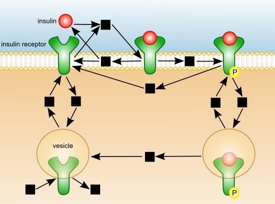
1. Introduction


2. Methods
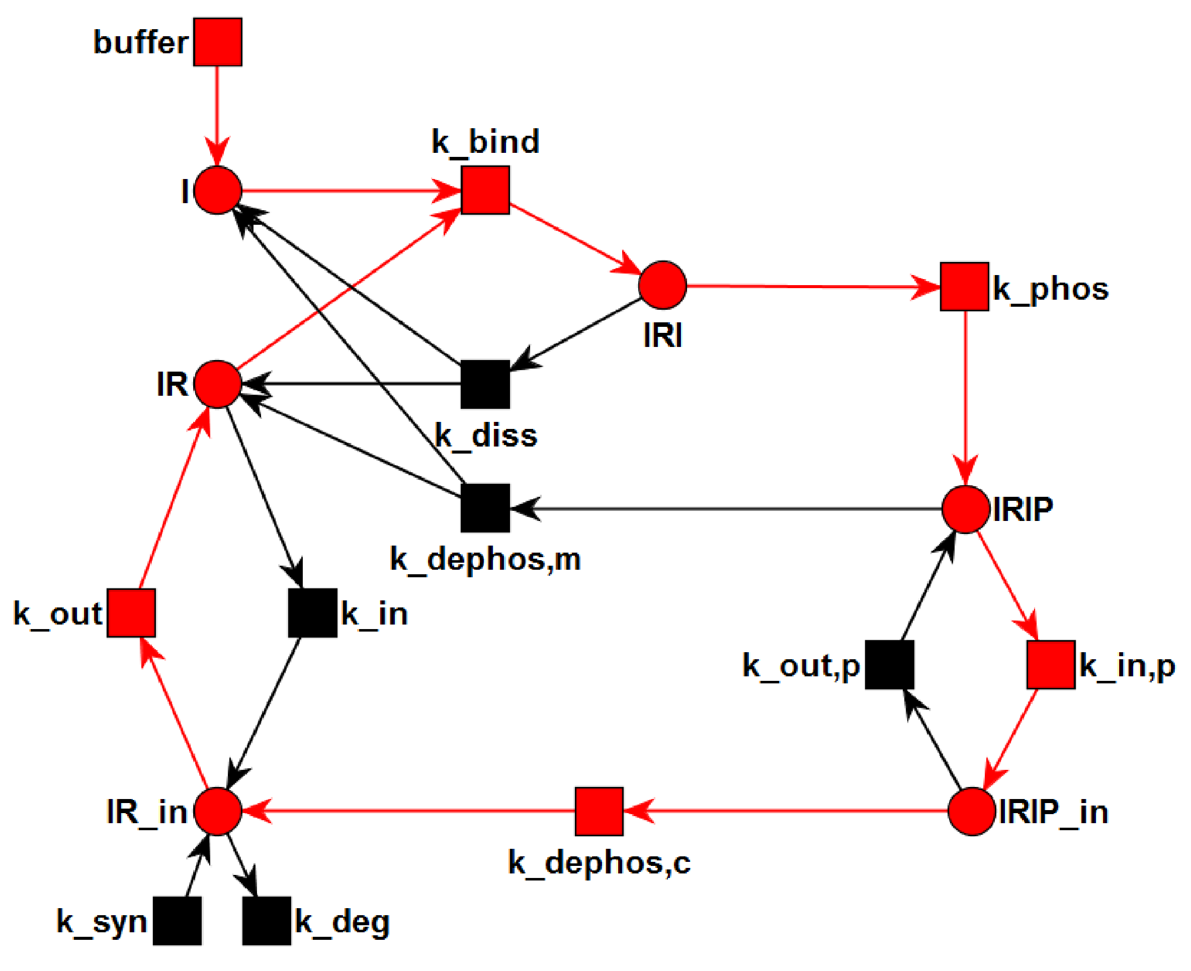
2.1. Petri Nets
- P is a finite set of places,
- T is a finite set of transitions,
- is a set of edges,
- is the set of edge weights, and
- is the initial marking.
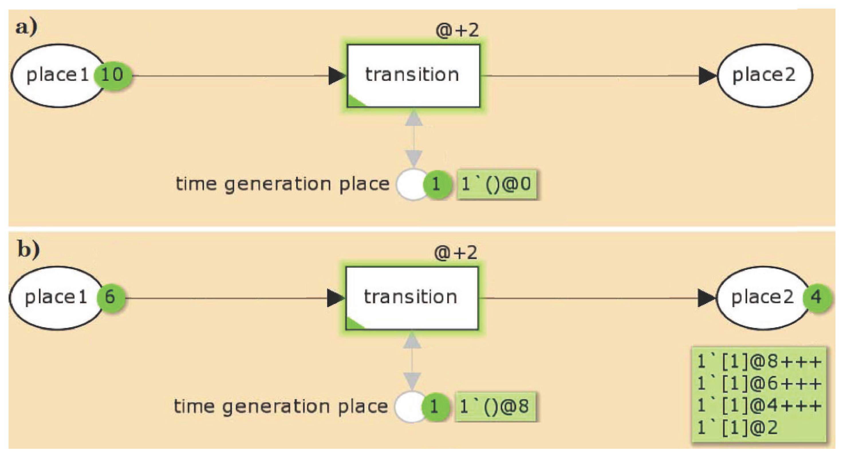
2.1.1. Timed Petri Nets

2.1.2. General Properties
2.1.3. Invariant Properties
3. Results and Discussion

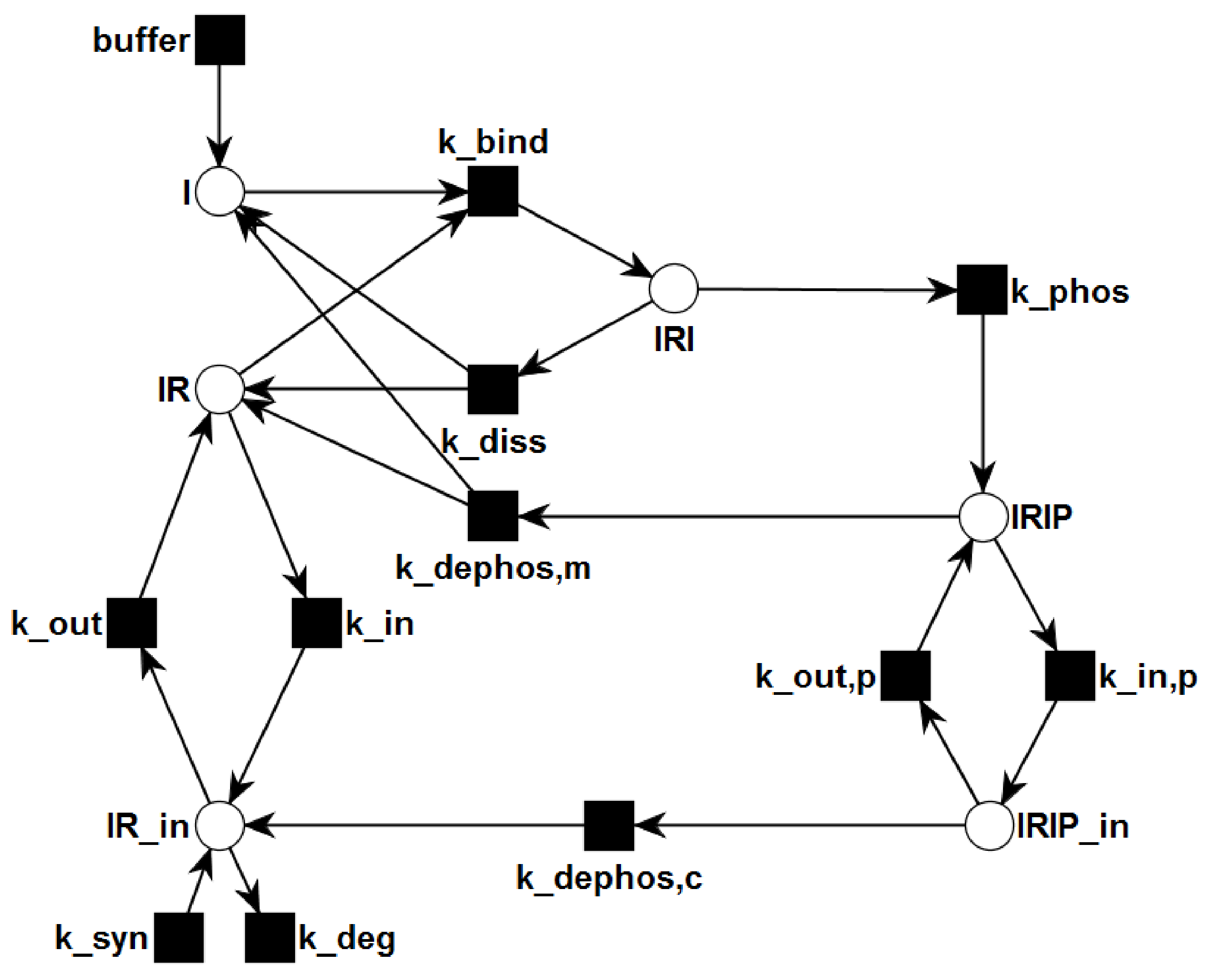
| Abbreviation | Species | Initial Concentration(s) [pM] |
|---|---|---|
| I | insulin | [I]– |
| IR | insulin receptor | [IR] |
| IRI | I-IR complex | — |
| IRIP | phosphorylated IRI | — |
| IRIP | intracellular IRIP | — |
| IR | intracellular IR | [IR] |
| Parameter | Process | Value | Units |
|---|---|---|---|
| binding of insulin | M min | ||
| dissociation of insulin | min | ||
| phosphorylation | min | ||
| dephosphorylation on membrane | min | ||
| internalization of IR | min | ||
| transport of IR to plasma membrane | min | ||
| internalization of phosphorylated IR | min | ||
| transport of phosphorylated IR to plasma membrane | min | ||
| dephosphorylation in cytoplasm | min | ||
| degradation | min | ||
| synthesis | M min | ||
| M min |
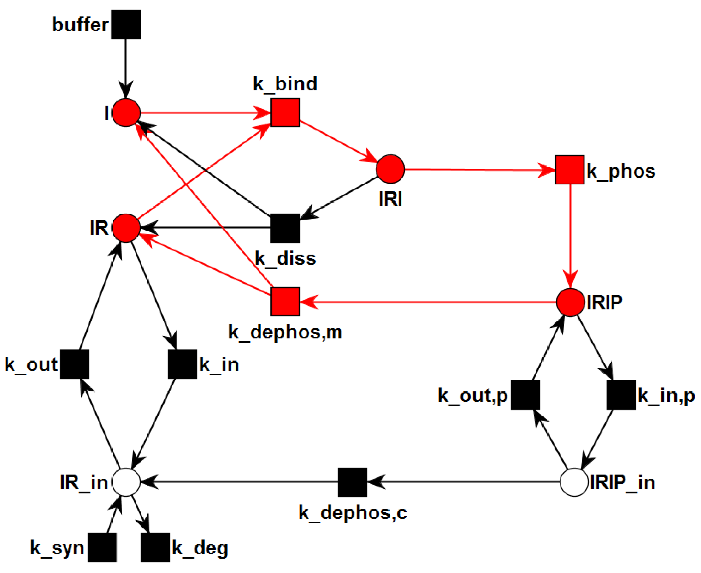
3.1. The P/T-PN Model and Its Properties
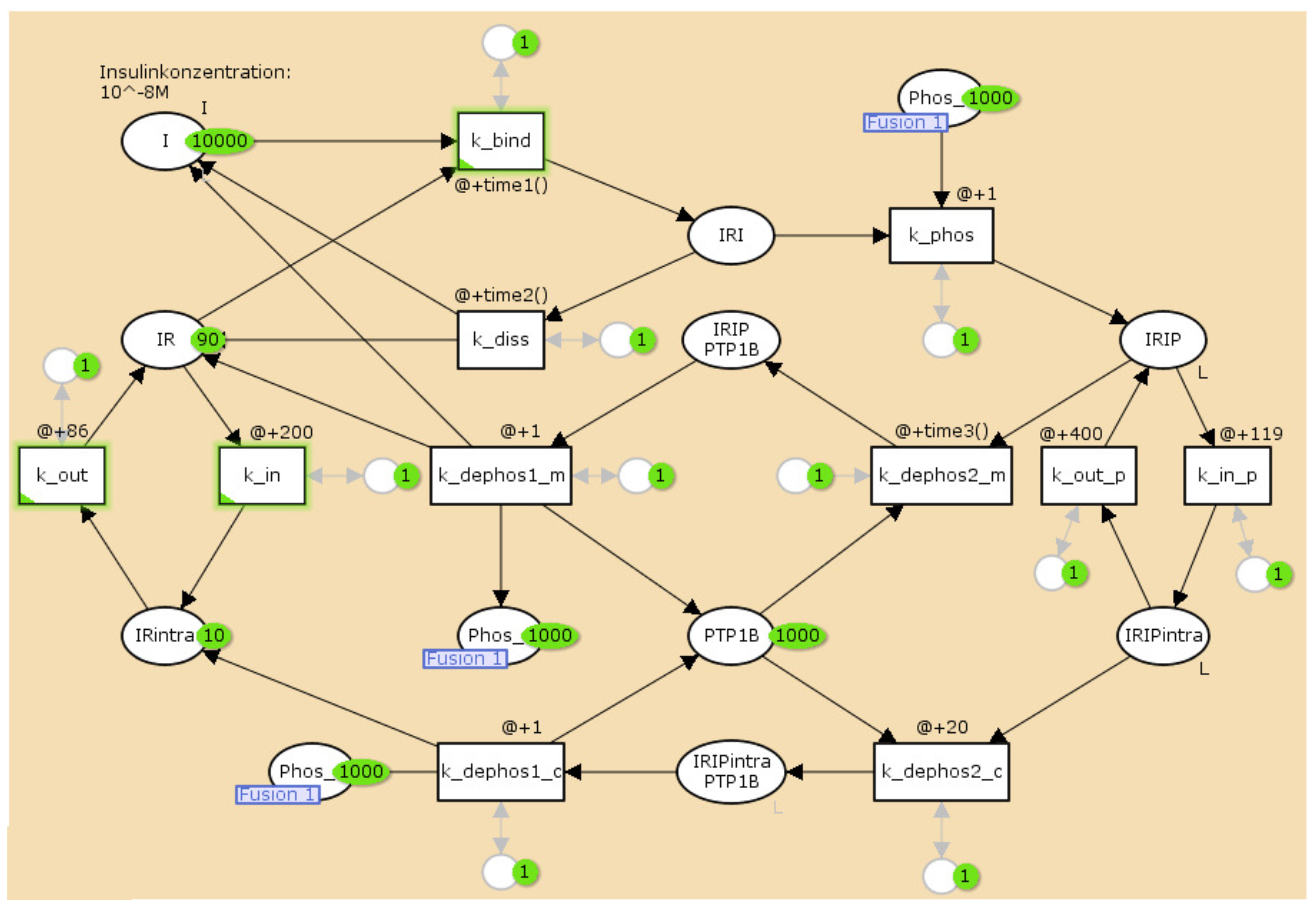
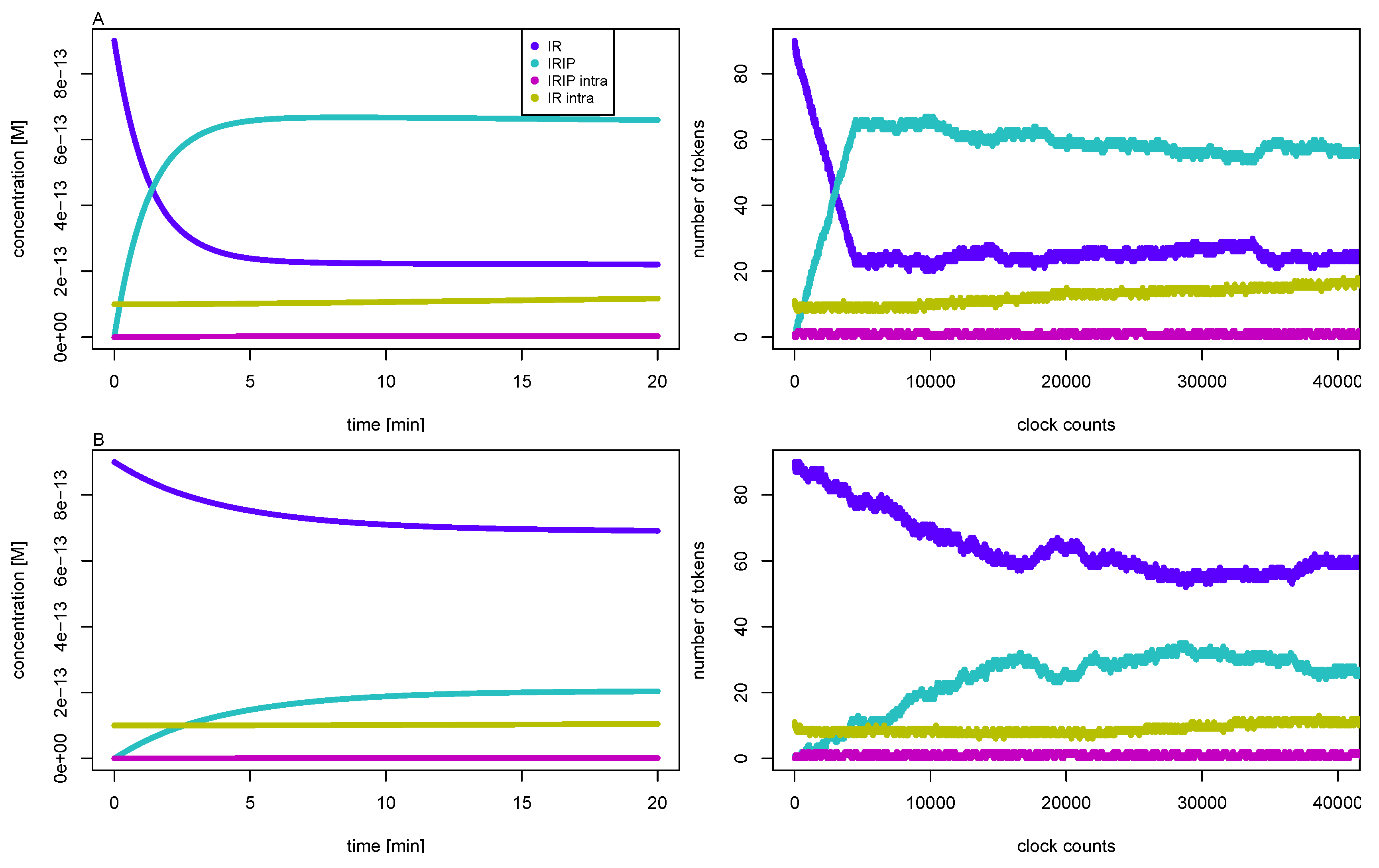
3.2. The TPN Model and Its Properties

| Name | Molecule | Initial Number of Tokens |
|---|---|---|
| I | insulin | 10,000 |
| IR | insulin receptor | 90 |
| IRI | I–IR complex | 0 |
| IRIP | phosphorylated IRI | 0 |
| IRIP | intracellular IRIP | 0 |
| IR | intracellular IR | 10 |
| PTPN1B | protein-tyrosine phosphatase 1B | 1000 |
| IRIP PTP1B | IRIP–PTPN1B complex | 0 |
| IRIP PTPN1B | IRIP–PTPN1B complex | 0 |
| Phos | phosphate | 1000 |
| Name | Process | Time Inscription |
|---|---|---|
| bin_1 | binding of insulin | @ + 1 |
| dis_1 | dissociation of insulin | @ + 40 |
| autophos_1 | phosphorylation of IRI | @ + 1 |
| intra_1 | internalization of IR | @ + 200 |
| memb_1 | transport of IR to plasma membrane | @ + 85 |
| intra_2 | internalization of IRIP | @ + 110 |
| memb_2 | transport of IRIP to plasma membrane | @ + 400 |
| dephos_1 | dephosphorylation of IRIP by PTPN1B | @ + 1 |
| dephos_2 | IRIP binds to PTPN1B | @ + 40 |
| dephos_3 | IRIP binds to PTPN1B | @ + 20 |
| dephos_4 | dephosphorylation of IRIP by PTPN1B | @ + 1 |
| Transition | 1 μM | 100 nM | 10 nM | 1 nM |
|---|---|---|---|---|
| bin_1 | @ + 1 | @ + 7 | @ + 16 (@ + 29) | @ + 20 (@ + 30) |
| dis_1 | @ + 40 | @ + 40 | @ + 40 (@ + 39) | @ + 40 (@ + 60) |
| memb_1 | @ + 85 | @ + 85 | @ + 86 | @ + 86 |
| intra_2 | @ + 110 | @ + 110 | @ + 119 | @ + 119 |
| dephos_2 | @ + 40 | @ + 40 | @ + 40 (@ + 52) | @ + 40 (@ + 65) |

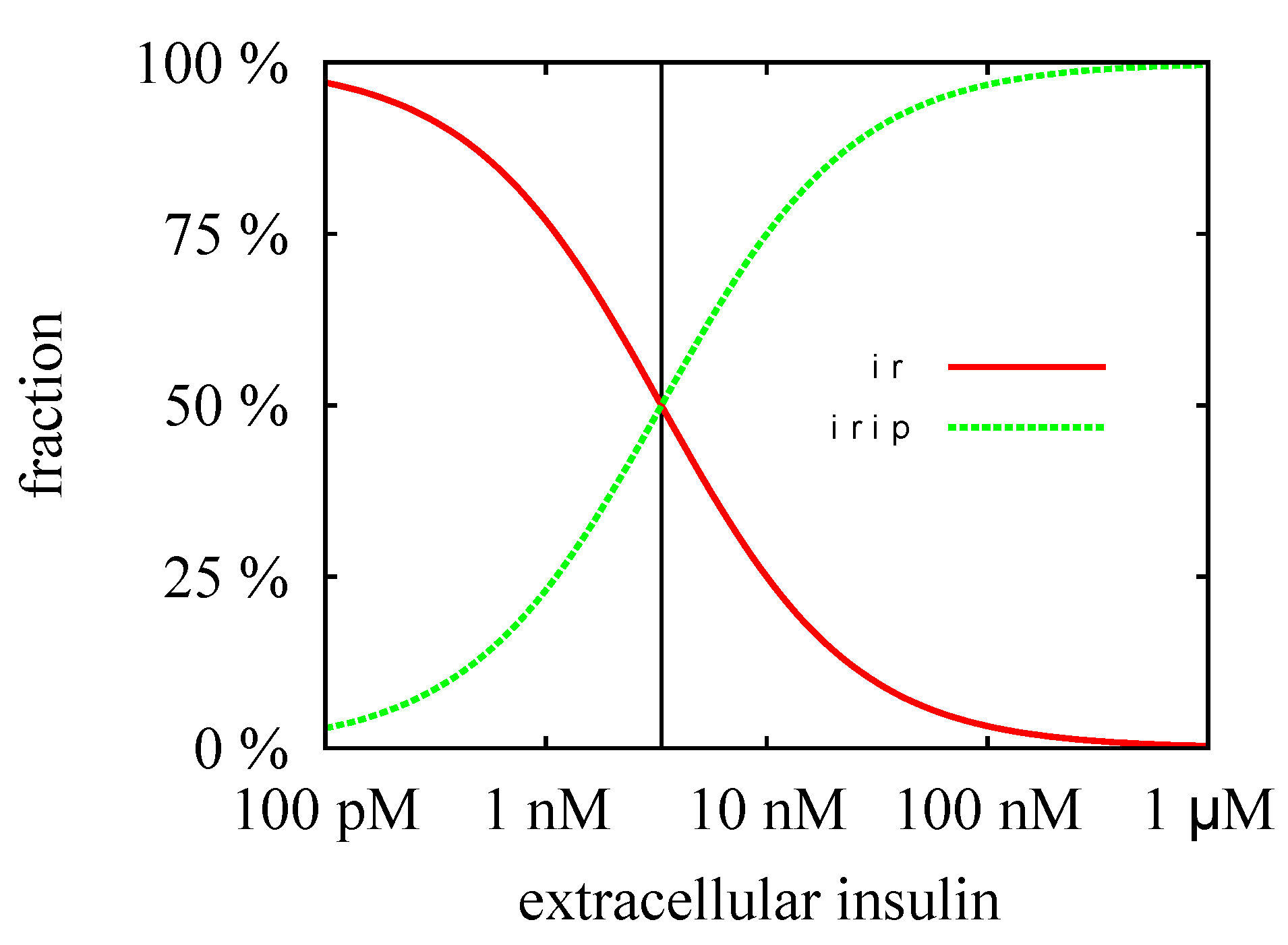
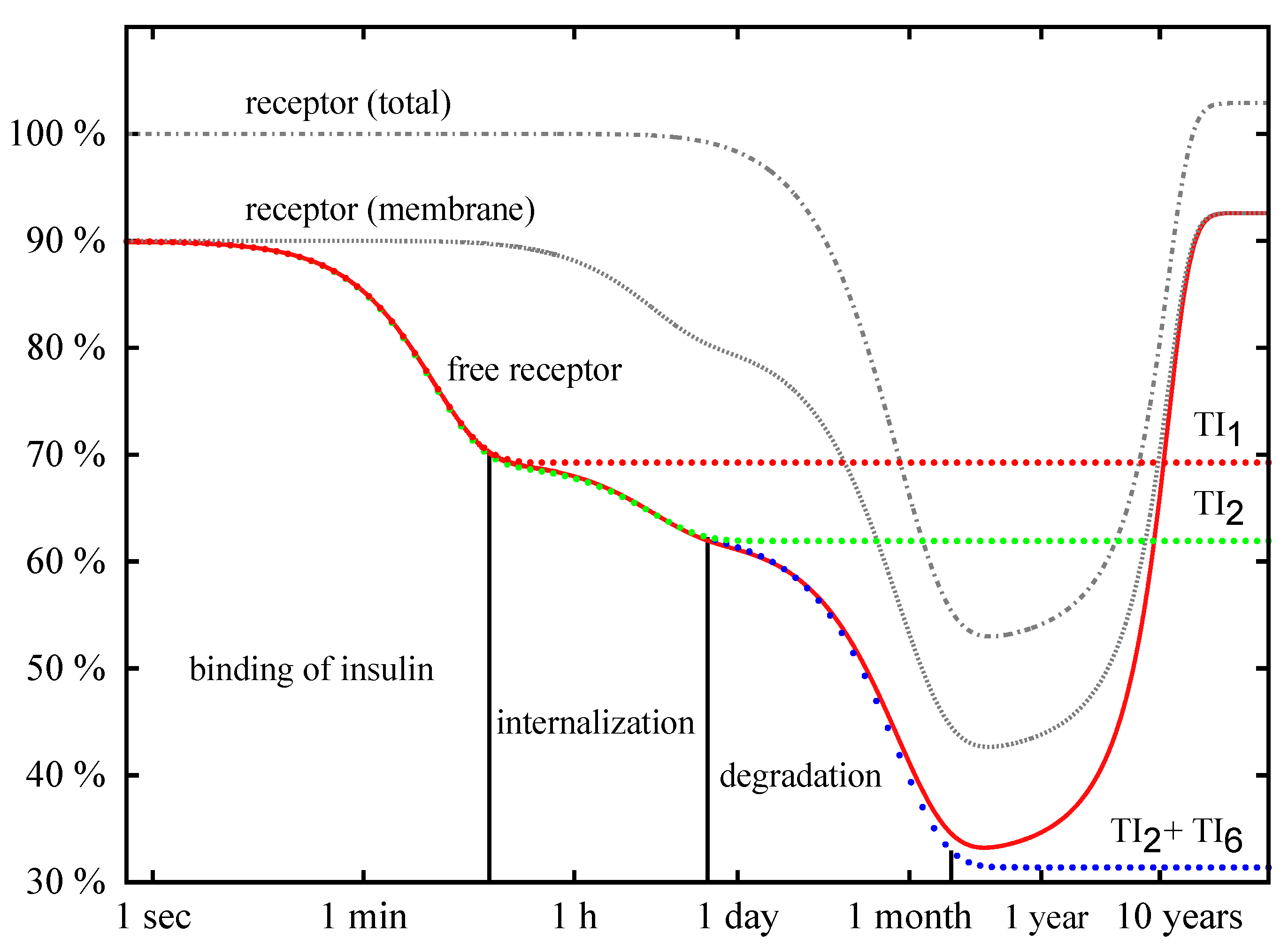
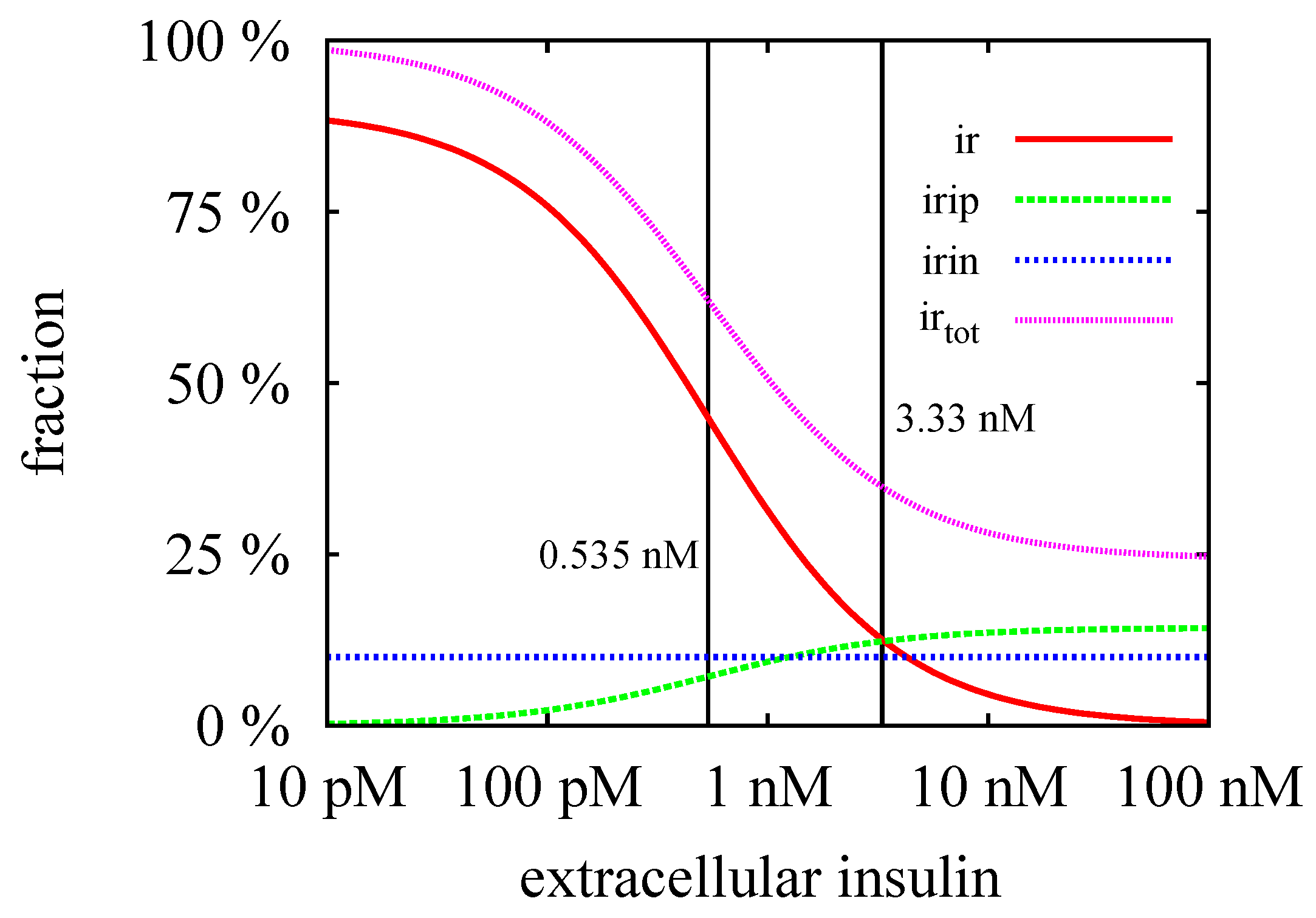
3.3. Quasi-Steady-State Approximation

Time Behavior
4. Conclusions
Supplementary Materials
Acknowledgments
Author Contributions
Conflicts of Interest
References
- Reaven, G.M. Role of insulin resistance in human disease. Diabetes 1988, 37, 1595–1607. [Google Scholar] [CrossRef] [PubMed]
- López-Otín, C.; Blasco, M.A.; Partridge, L.; Serrano, M.; Kroemer, G. The hallmarks of aging. Cell 2013, 153, 1194–1217. [Google Scholar] [CrossRef] [PubMed]
- Cohen, E.; Dillin, A. The insulin paradox: Aging, proteotoxicity and neurodegeneration. Nat. Rev. Neurosci. 2008, 9, 759–767. [Google Scholar] [CrossRef] [PubMed]
- Schäffer, L. A model for insulin binding to the insulin receptor. Eur. J. Biochem. 1994, 221, 1127–1132. [Google Scholar] [CrossRef] [PubMed]
- Subramanian, K.; Fee, C.J.; Fredericks, R.; Stubbs, R.S.; Hayes, M.T. Insulin receptor-insulin interaction kinetics using multiplex surface plasmon resonance. J. Mol. Recognit. 2013, 26, 643–652. [Google Scholar] [CrossRef] [PubMed]
- Menting, J.G.; Whittaker, J.; Margetts, M.B.; Whittaker, L.J.; Kong, G.K.W.; Smith, B.J.; Watson, C.J.; Žáková, L.; Kletvíková, E.; Jirácek, J.; et al. How insulin engages its primary binding site on the insulin receptor. Nature 2013, 493, 241–245. [Google Scholar] [CrossRef] [PubMed]
- Saltiel, A.; Kahn, R. Insulin signalling and the regulation of glucose and lipid metabolism. Nature 2001, 414, 799–806. [Google Scholar] [CrossRef] [PubMed]
- Bouzakri, K.; Koistinen, H.; Zierath, J. Molecular mechanisms of skeletal muscle insulin resistance in type 2 diabetes. Curr. Diabetes Rev. 2005, 1, 167–174. [Google Scholar] [CrossRef] [PubMed]
- Duckworth, W.C.; Bennett, R.G.; Hamel, F.G. Insulin degradation: Progress and potential. Endocr. Rev. 1998, 19, 608–624. [Google Scholar] [CrossRef] [PubMed]
- Thorsøe, K.; Schlein, M.; Steensgaard, D.; Brandt, J.; Schluckebier, G.; Naver, H. Kinetic evidence for the sequential association of insulin binding site 1 and 2 to the insulin receptor and the influence of receptor isoform. Biochemistry 2010, 49, 6234–6246. [Google Scholar] [CrossRef] [PubMed]
- De Meyts, P.; Roth, J.; Neville, D.M., Jr.; Gavin, J.R., III; Lesniak, M.A. Insulin interactions with its receptors: Experimental evidence for negative cooperativity. Biochem. Biophys. Res. Commun. 1973, 55, 154–161. [Google Scholar] [CrossRef]
- Winter, P.W.; McPhee, J.T.; van Orden, A.K.; Roess, D.A.; Barisas, B.G. Fluorescence correlation spectroscopic examination of insulin and insulin-like growth factor 1 binding to live cells. Biophys. Chem. 2011, 159, 303–310. [Google Scholar] [CrossRef] [PubMed]
- Hua, Q. Insulin: A small protein with a long journey. Protein Cell 2010, 1, 537–551. [Google Scholar] [CrossRef] [PubMed]
- Ward, C.W.; Menting, J.G.; Lawrence, M.C. The insulin receptor changes conformation in unforeseen ways on ligand binding: Sharpening the picture of insulin receptor activation. BioEssays 2013, 35, 945–954. [Google Scholar] [CrossRef] [PubMed]
- Corin, R.; Donner, D. Insulin receptors convert to a higher affinity state subsequent to hormone binding. A two-state model for the insulin receptor. J. Biol. Chem. 1982, 257, 104–110. [Google Scholar] [PubMed]
- Jeffrey, P. The interaction of insulin with its receptor: Cross-linking via insulin association as the source of receptor clustering. Diabetologia 1982, 23, 381–385. [Google Scholar] [CrossRef] [PubMed]
- Kohanski, R. Insulin receptor autophosphorylation. I. Autophosphorylation kinetics of the native receptor and its cytoplasmic kinase domain. Biochemistry 1993, 32, 5766–5772. [Google Scholar] [CrossRef] [PubMed]
- Hammond, B.J.; Tikerpae, J.; Smith, G.D. An evaluation of the cross—Linking model for the interaction of insulin with its receptor. Am. J. Physiol. Endocrinol. Metab. 1997, 272, E1136–E1144. [Google Scholar]
- Wanant, S.; Quon, M.J. Insulin receptor binding kinetics: Modeling and simulation studies. J. Theor. Biol. 2000, 205, 355–364. [Google Scholar] [CrossRef] [PubMed]
- Kiselyov, V.; Versteyhe, S.; Gauguin, L.; de Meyts, P. Harmonic oscillator model of the insulin and IGF1 receptors allosteric binding and activation. Mol. Syst. Biol. 2009, 5, 1–12. [Google Scholar] [CrossRef] [PubMed]
- Louise, K.; Pierre, D.M.; Vladislav, V.K. Insight into the molecular basis for the kinetic differences between the two insulin receptor isoforms. Biochem. J. 2011, 440, 397–403. [Google Scholar]
- Desbuquois, B.; Lopez, S.; Burlet, H. Ligand-induced translocation of insulin receptors in intact rat liver. J. Biol. Chem. 1982, 257, 10852–10860. [Google Scholar] [PubMed]
- Giudice, J.; Jares-Erijman, E.A.; Leskow, F.C. Endocytosis and intracellular dissociation rates of human insulin-insulin receptor complexes by quantum dots in living cells. Bioconjug. Chem. 2013, 24, 431–442. [Google Scholar] [CrossRef] [PubMed]
- Amaya, M.J.; Oliveira, A.G.; Guimarães, E.S.; Casteluber, M.C.; Carvalho, S.M.; Andrade, L.M.; Pinto, M.C.; Mennone, A.; Oliveira, C.A.; Resende, R.R.; et al. The insulin receptor translocates to the nucleus to regulate cell proliferation in liver. Hepatology 2014, 59, 274–283. [Google Scholar] [CrossRef] [PubMed]
- Chang, M.; Kwon, M.; Kim, S.; Yunn, N.O.; Kim, D.; Yunn, N.-O.; Kim, D.; Ryu, S.H.; Lee, J.-B. Aptamer-based single-molecule imaging of insulin receptors in living cells. J. Biomed. Opt. 2013, 19, 051204–051204. [Google Scholar] [CrossRef] [PubMed]
- Fagerholm, S.; Örtegren, U.; Karlsson, M.; Ruishalme, I.; Strålfors, P. Rapid insulin-dependent endocytosis of the insulin receptor by caveolae in primary adipocytes. PLoS ONE 2009, 4, e5985. [Google Scholar] [CrossRef] [PubMed] [Green Version]
- Makroglou, A.; Li, J.; Kuang, Y. Mathematical models and software tools for the glucose-insulin regulatory system and diabetes: An overview. Appl. Numer. Math. 2006, 56, 559–573. [Google Scholar] [CrossRef]
- Standaert, M.; Pollet, R. Equilibrium model for insulin-induced receptor down-regulation. regulation of insulin receptors in differentiated BC3H-1 myocytes. J. Biol. Chem. 1984, 259, 2346–2354. [Google Scholar] [PubMed]
- Backer, J.M.; Kahn, C.R.; White, M. Tyrosine phosphorylation of the insulin receptor during insulin-stimulated internalization in rat hepatoma cells. J. Biol. Chem. 1989, 264, 1694–1701. [Google Scholar] [PubMed]
- Sturis, J.; Polonsky, K.S.; Mosekilde, E.; van Cauter, E. Computer model for mechanisms underlying ultradian oscillations of insulin and glucose. Am. J. Physiol. Endocrinol. Metab. 1991, 260, E801–E809. [Google Scholar]
- Quon, M.J.; Campfield, L.A. A mathematical model and computer simulation study of insulin receptor regulation. J. Theor. Biol. 1991, 150, 59–72. [Google Scholar] [CrossRef]
- Shymko, R.; Dumont, E.; de Meyts, P.; Dumont, J. Timing-dependence of insulin-receptor mitogenic versus metabolic signalling: A plausible model based on coincidence of hormone and effector binding. Biochem. J. 1999, 339, 675–683. [Google Scholar] [CrossRef] [PubMed]
- Tolić, I.; Mosekilde, E.; Sturis, J. Modeling the insulin-glucose feedback system: The significance of pulsatile insulin secretion. J. Theor. Biol. 2000, 207, 361–375. [Google Scholar] [CrossRef] [PubMed]
- Sedaghat, A.R.; Sherman, A.; Quon, M.J. A mathematical model of metabolic insulin signaling pathways. Am. J. Physiol. Endocrinol. Metab. 2002, 283, E1084–E1101. [Google Scholar] [CrossRef] [PubMed]
- Giri, L.; Mutalik, V.K.; Venkatesh, K. A steady state analysis indicates that negative feedback regulation of PTP1B by Akt elicits bistability in insulin-stimulated GLUT4 translocation. Theor. Biol. Med. Model. 2004, 1, 2. [Google Scholar] [CrossRef] [PubMed] [Green Version]
- Hori, S.S.; Kurland, I.J.; DiStefano, J.J., III. Role of endosomal trafficking dynamics on the regulation of hepatic insulin receptor activity: Models for Fao cells. Ann. Biomed. Eng. 2006, 34, 879–892. [Google Scholar] [CrossRef] [PubMed]
- Koschorrek, M.; Gilles, E. Mathematical modeling and analysis of insulin clearance in vivo. BMC Syst. Biol. 2008, 2, 1–18. [Google Scholar] [CrossRef] [PubMed]
- Liu, W.; Tang, F. Modeling a simplified regulatory system of blood glucose at molecular levels. J. Theor. Biol. 2008, 252, 608–620. [Google Scholar] [CrossRef] [PubMed]
- Cedersund, G.; Roll, J.; Ulfhielm, E.; Danielsson, A.; Tidefelt, H.; Strålfors, P. Model-based hypothesis testing of key mechanisms in initial phase of insulin signaling. PLoS Comput. Biol. 2008, 4, e1000096. [Google Scholar] [CrossRef] [PubMed]
- Cedersund, G.; Roll, J. Systems biology: Model based evaluation and comparison of potential explanations for given biological data. FEBS J. 2009, 276, 903–922. [Google Scholar] [CrossRef] [PubMed]
- Liu, W.; Hsin, C.; Tang, F. A molecular mathematical model of glucose mobilization and uptake. Math. Biosci. 2009, 221, 121–129. [Google Scholar] [CrossRef] [PubMed]
- Chew, Y.H.; Shia, Y.L.; Lee, C.T.; Majid, F.A.A.; Chua, L.S.; Sarmidi, M.R.; Aziz, R.A. Modeling of glucose regulation and insulin-signaling pathways. Mol. Cell. Endocrinol. 2009, 303, 13–24. [Google Scholar] [CrossRef] [PubMed]
- Sogaard, P.; Szekeres, F.; Garcia-Roves, P.; Larsson, D.; Chibalin, A.; Zierath, J.R. Spatial insulin signalling in isolated skeletal muscle preparations. J. Cell. Biochem. 2010, 109, 943–949. [Google Scholar] [CrossRef] [PubMed]
- Brännmark, C.; Palmér, R.; Glad, S.T.; Cedersund, G.; Strålfors, P. Mass and information feedbacks through receptor endocytosis govern insulin signaling as revealed using a parameter-free modeling framework. J. Biol. Chem. 2010, 285, 20171–20179. [Google Scholar] [CrossRef] [PubMed]
- Nyman, E.; Brännmark, C.; Palmér, R.; Brugård, J.; Nyström, F.H.; Cedersund, G.; Strålfors, P. A hierarchical wholebody modeling approach elucidates the link between in vitro insulin signaling and in vivo glucose homeostasis. J. Biol. Chem. 2011, 286, 26028–26041. [Google Scholar] [CrossRef] [PubMed]
- Nyman, E.; Cedersund, G.; Strålfors, P. Insulin signaling-mathematical modeling comes of age. Trends Endocrinol. Metab. 2012, 23, 107–115. [Google Scholar] [CrossRef] [PubMed]
- Cedersund, G. Conclusions via unique predictions obtained despite unidentifiability-new definitions and a general method. FEBS J. 2012, 279, 3513–3527. [Google Scholar] [CrossRef] [PubMed]
- Berestovsky, N.; Zhou, W.; Nagrath, D.; Nakhleh, L. Modeling integrated cellular machinery using hybrid Petri-Boolean networks. PLoS Comput. Biol. 2013, 9, e1003306. [Google Scholar] [CrossRef] [PubMed]
- Garcia-Gabin, W.; Jacobsen, E.W. Multilevel model of type 1 diabetes mellitus patients for model-based glucose controllers. J. Diabetes Sci. Technol. 2013, 7, 193–201. [Google Scholar] [CrossRef] [PubMed]
- Brännmark, C.; Nyman, E.; Fangerholm, S.; Bergenholm, L.; Ekstrand, E.M.; Cedersund, G.; Strålfors, P. Insulin signaling in type 2 diabetis. J. Biol. Chem. 2013, 288, 9876–9880. [Google Scholar]
- Smith, G.R.; Shanley, D.P. Computational modelling of the regulation of insulin signalling by oxidative stress. BMC Syst. Biol. 2013, 7, 41. [Google Scholar] [CrossRef] [PubMed]
- Ajmera, I.; Swat, M.; Laibe, C.; le Novère, N.; Chelliah, V. The impact of mathematical modeling on the understanding of diabetes and related complications. CPT Pharmacomet. Syst. Pharmacol. 2013, 2, e54. [Google Scholar] [CrossRef] [PubMed]
- Bevan, A.P.; Drake, P.G.; Bergeron, J.J.; Posner, B.I. Intracellular signal transduction: The role of endosomes. Trends Endocrinol. Metab. 1996, 7, 13–21. [Google Scholar] [CrossRef]
- Goh, L.K.; Sorkin, A. Endocytosis of receptor tyrosine kinases. Cold Spring Harb. Perspect. Biol. 2013, 5, a017459. [Google Scholar] [CrossRef] [PubMed]
- Song, R.; Peng, W.; Zhang, Y.; Lv, F.; Wu, H.K.; Guo, J.; Cao, Y.; Pi, Y.; Zhang, X.; Jin, L.; et al. Central role of E3 ubiquitin ligase MG53 in insulin resistance and metabolic disorders. Nature 2013, 494, 375–379. [Google Scholar] [CrossRef] [PubMed]
- Olefsky, J.M. Decreased insulin binding to adipocytes and circulating monocytes from obese subjects. J. Clin. Investig. 1976, 57, 1165–1172. [Google Scholar] [CrossRef] [PubMed]
- Kolterman, O.; Insel, J.; Saekow, M.; Olefsky, J. Mechanisms of insulin resistance in human obesity: Evidence for receptor and postreceptor defects. J. Clin. Investig. 1980, 65, 1272–1284. [Google Scholar] [CrossRef] [PubMed]
- Kolterman, O.; Gray, R.; Griffin, J.; Burstein, P.; Insel, J.; Scarlett, J.A.; Olefsky, J.M. Receptor and postreceptor defects contribute to the insulin resistance in noninsulin-dependent diabetes mellitus. J. Clin. Investig. 1981, 68, 957–969. [Google Scholar] [CrossRef] [PubMed]
- Friedman, J.E.; Ishizuka, T.; Liu, S.; Farrell, C.J.; Bedol, D.; Koletsky, R.J.; Kaung, H.-L.; Ernsberger, P. Reduced insulin receptor signaling in the obese spontaneously hypertensive Koletsky rat. Am. J. Physiol. Endocrinol. Metab. 1997, 273, E1014–E1023. [Google Scholar]
- Danielsson, A.; Fagerholm, S.; Öst, A.; Franck, N.; Kjolhede, P.; Nystrom, F.H.; Strålfors, P. Short-term overeating induces insulin resistance in fat cells in lean human subjects. Mol. Med. 2009, 15, 228–234. [Google Scholar] [CrossRef] [PubMed]
- Petri, C.A. Kommunikation mit Automaten. Ph.D. Thesis, University of Bonn, Bonn, Germany, 1962. [Google Scholar]
- Murata, T. Petri nets: Properties, analysis and applications. Proc. IEEE Int. Conf. Consum. Electron. 1989, 77, 541–580. [Google Scholar] [CrossRef]
- Koch, I.; Reisig, W.; Schreiber, F. Modeling in Systems Biology: The Petri Net Approach; Computational Biology; Dress, A., Vingron, M., Eds.; Springer-Verlag: London, UK, 2011; Volume 16. [Google Scholar]
- Reisig, W. Petri Nets: An Introduction. In EATCS Monographs on Theoretical Computer Science; Springer-Verlag: Berlin, Germany; Heidelberg, Germany, 1985; Volume 4. [Google Scholar]
- Haken, H. Synergetics. An Introduction; Springer-Verlag: Berlin, Germany; Heidelberg, Germany; New York, NY, USA, 1977. [Google Scholar]
- Murray, J.D. Mathematical Biology, 2nd ed.; Springer-Verlag: Berlin, Germany, 1993. [Google Scholar]
- Deuflhard, P.; Bornemann, F. Scientific Computing with Ordinary Differential Equations; Springer-Verlag: New York, NY, USA, 2002; Volume 42. [Google Scholar]
- Gillespie, D.T. Exact stochastic simulation of coupled chemical reactions. J. Phys. Chem. 1977, 81, 2340–2361. [Google Scholar] [CrossRef]
- Gardiner, C.W. Handbook of Stochastic Methods; Springer-Verlag: Berlin, Germany, 1985; Volume 3. [Google Scholar]
- Wilkinson, D.J. Stochastic Modelling for Systems Biology; CRC Press: London, UK; New York, NY, USA, 2011. [Google Scholar]
- Gray, C. Sensitivity Analysis of the Insulin Signalling Pathway for Glucose Transport. Master’s Thesis, School of Mathematics and Statistics, The University of New South Wales, Pontypridd, UK, 2013. [Google Scholar]
- Gavin, J.R.; Roth, J.; Neville, D.M.; de Meyts, P.; Buell, D.N. Insulin-dependent regulation of insulin receptor concentrations: A direct demonstration in cell culture. Proc. Natl. Acad. Sci. USA 1974, 71, 84–88. [Google Scholar] [CrossRef] [PubMed]
- Kosmakos, F.; Roth, J. Insulin-induced loss of the insulin receptor in IM-9 lymphocytes. A biological process mediated through the insulin receptor. J. Biol. Chem. 1980, 255, 9860–9869. [Google Scholar] [PubMed]
- Kasuga, M.; Kahn, C.R.; Hedo, J.A.; van Obberghen, E.; Yamada, K.M. Insulin-induced receptor loss in cultured human lymphocytes is due to accelerated receptor degradation. Proc. Natl. Acad. Sci. USA 1981, 78, 6917–6921. [Google Scholar] [CrossRef] [PubMed]
- Krupp, M.; Lane, M.D. On the mechanism of ligand-induced down-regulation of insulin receptor level in the liver cell. J. Biol. Chem. 1981, 256, 1689–1694. [Google Scholar] [PubMed]
- Ronnett, G.; Knutson, V.; Lane, M. Insulin-induced down-regulation of insulin receptors in 3T3-L1 adipocytes. Altered rate of receptor inactivation. J. Biol. Chem. 1982, 257, 4285–4291. [Google Scholar] [PubMed]
- Green, A.; Olefsky, J.M. Evidence for insulin-induced internalization and degradation of insulin receptors in rat adipocytes. Proc. Natl. Acad. Sci. USA 1982, 79, 427–431. [Google Scholar] [CrossRef] [PubMed]
- Berhanu, P.; Olefsky, J.M.; Tsai, P.; Thamm, P.; Saunders, D.; Brandenburg, D. Internalization and molecular processing of insulin receptors in isolated rat adipocytes. Proc. Natl. Acad. Sci. USA 1982, 79, 4069–4073. [Google Scholar] [CrossRef] [PubMed]
- Marshall, S. Kinetics of insulin receptor biosynthesis and membrane insertion: Relationship to cellular function. Diabetes 1983, 32, 319–325. [Google Scholar] [CrossRef] [PubMed]
- Marshall, S.; Garvey, W.T.; Geller, M. Primary culture of isolated adipocytes. A new model to study insulin receptor regulation and insulin action. J. Biol. Chem. 1984, 259, 6376–6384. [Google Scholar] [PubMed]
- Marshall, S. Kinetics of insulin receptor internalization and recycling in adipocytes. Shunting of receptors to a degradative pathway by inhibitors of recycling. J. Biol. Chem. 1985, 260, 4136–4144. [Google Scholar] [PubMed]
- Knutson, V.; Ronnett, G.; Lane, M. The effects of cycloheximide and chloroquine on insulin receptor metabolism. Differential effects on receptor recycling and inactivation and insulin degradation. J. Biol. Chem. 1985, 260, 14180–14188. [Google Scholar] [PubMed]
- Kahn, C.R.; White, M. The insulin receptor and the molecular mechanism of insulin action. J. Clin. Investig. 1988, 82, 1151–1156. [Google Scholar] [CrossRef] [PubMed]
- Brunetti, A.; Maddux, B.; Wong, K.; Goldfine, I. Muscle cell differentiation is associated with increased insulin receptor biosynthesis and messenger RNA levels. J. Clin. Investig. 1989, 83, 192–198. [Google Scholar] [CrossRef] [PubMed]
- Trischitta, V.; Wong, K.Y.; Brunetti, A.; Scalisi, R.; Vigneri, R.; Goldfine, I.D. Endocytosis, recycling, and degradation of the insulin receptor. Studies with monoclonal antireceptor antibodies that do not activate receptor kinase. J. Biol. Chem. 1989, 264, 5041–5046. [Google Scholar] [PubMed]
- Haft, C.R.; Klausner, R.D.; Taylor, S.I. Involvement of dileucine motifs in the internalization and degradation of the insulin receptor. J. Biol. Chem. 1994, 269, 26286–26294. [Google Scholar] [PubMed]
- Capozza, F.; Combs, T.P.; Cohen, A.W.; Cho, Y.R.; Park, S.Y.; Schubert, W.; Williams, T.M.; Brasaemle, D.L.; Jelicks, L.A.; Scherer, P.E.; et al. Caveolin-3 knockout mice show increased adiposity and whole body insulin resistance, with ligand-induced insulin receptor instability in skeletal muscle. Am. J. Physiol. Cell Physiol. 2005, 288, C1317–C1331. [Google Scholar] [CrossRef] [PubMed]
- Ramos, F.J.; Langlais, P.R.; Hu, D.; Dong, L.Q.; Liu, F. Grb10 mediates insulin-stimulated degradation of the insulin receptor: A mechanism of negative regulation. Am. J. Physiol. Endocrinol. Metab 2006, 290, E1262–E1266. [Google Scholar] [CrossRef] [PubMed]
- Zhou, L.; Zhang, J.; Fang, Q.; Liu, M.; Liu, X.; Jia, W.; Dong, L.Q.; Liu, F. Autophagy-mediated insulin receptor down-regulation contributes to endoplasmic reticulum stress-induced insulin resistance. Mol. Pharmacol. 2009, 76, 596–603. [Google Scholar] [CrossRef] [PubMed]
- González-Muñoz, E.; Lopez-Iglesias, C.; Calvo, M.; Palacín, M.; Zorzano, A.; Camps, M. Caveolin-1 loss of function accelerates glucose transporter 4 and insulin receptor degradation in 3T3-L1 adipocytes. Endocrinology 2009, 150, 3493–3502. [Google Scholar] [CrossRef] [PubMed] [Green Version]
- Mayer, C.M.; Belsham, D.D. Central insulin signaling is attenuated by long-term insulin exposure via insulin receptor substrate-1 serine phosphorylation, proteasomal degradation, and lysosomal insulin receptor degradation. Endocrinology 2010, 151, 75–84. [Google Scholar] [CrossRef] [PubMed]
- Popova-Zeugmann, L. Time and Petri Nets: An Introduction; Springer-Verlag: Berlin, Germany; Heidelberg, Germany, 2013. [Google Scholar]
- Jensen, K. Coloured Petri Nets: Basic Concepts, Analysis Methods and Practical Use; Springer-Verlag: Berlin, Germany; Heidelberg, Germany, 1997; Volume 2. [Google Scholar]
- Ratzer, A.V.; Wells, L.; Lassen, H.M.; Laursen, M.; Qvortrup, J.F.; Stissing, M.S.; Westergaard, M.; Christensen, S.; Jensen, K. CPN tools for editing, simulating, and analysing coloured Petri nets. In Proceedings of the ICATPN’03 Proceedings of the 24th International Conference on Applications and Theory of Petri Nets, Eindhoven, The Netherlands, 23–27 June 2003; Springer-Verlag: Berlin, Germany; Heidelberg, Germany, 2003; pp. 450–462. [Google Scholar]
- Starke, P. Analyse von Petri-Netz-Modellen; G.G. Teubner-Verlag: Stuttgart, Germany, 1990. [Google Scholar]
- Balazki, P.; Lindauer, K.; Einloft, J.; Ackermann, J.; Koch, I. MonaLisa for stochastic simulations of Petri net models of biochemical systems. BMC Bioinform. 2015, 16, 215–226. [Google Scholar] [CrossRef] [PubMed]
- Balazki, P.; Lindauer, K.; Einloft, J.; Ackermann, J.; Koch, I. Erratum to: MonaLisa for stochastic simulations of Petri net models of biochemical systems. BMC Bioinform. 2015, 16, 371. [Google Scholar] [CrossRef] [PubMed]
- Corless, R.; Gonnet, G.; Hare, D.; Jeffrey, D.; Knuth, D. On the Lambert W function. Adv. Comput. Math. 1996, 5, 329–359. [Google Scholar] [CrossRef]
- Lautenbach, K. Exakte Bedingungen der Lebendigkeit für eine Klasse von Petri-Netzen; Report 82; Gesellschaft für Mathematik und Datenverarbeitung: Bonn, Germany, 1973. [Google Scholar]
- Colom, J.M.; Silva, M. Convex geometry and semiflows in P/T nets. A comparative study of algorithms for computation of minimal p-semiflows. In Advances in Petri Nets; Springer-Verlag: Berlin, Germany; Heidelberg, Germany, 1991; pp. 79–112. [Google Scholar]
- Fortunato, S. Community detection in graphs. Phys. Rep. 2010, 486, 75–174. [Google Scholar] [CrossRef]
- Shen, J.; Chen, Z.; Chen, C.; Zhu, X.; Han, Y. Impact of incretin on early-phase insulin secretion and glucose excursion. Endocrine 2013, 44, 403–410. [Google Scholar] [CrossRef] [PubMed]
- Brunetti, A.; Manfiolett, G.; Chiefari, E.; Goldfine, I.D.; Foti, D. Transcriptional regulation of human insulin receptor gene by the high-mobility group protein HMGI (Y). FASEB J. 2001, 15, 492–500. [Google Scholar] [CrossRef] [PubMed]
- Foti, D.; Iuliano, R.; Chiefari, E.; Brunetti, A. A nucleoprotein complex containing Sp1, C/EBP, and HMGI-Y controls human insulin receptor gene transcription. Mol. Cell. Biol. 2003, 23, 2720–2732. [Google Scholar] [CrossRef] [PubMed]
- Puig, O.; Tjian, R. Transcriptional feedback control of insulin receptor by dFOXO/FOXO1. Genes Dev. 2005, 19, 2435–2446. [Google Scholar] [CrossRef] [PubMed]
- Friedman, A.; Perrimon, N. A functional RNAi screen for regulators of receptor tyrosine kinase and ERK signalling. Nature 2006, 444, 230–234. [Google Scholar] [CrossRef] [PubMed]
- Sackmann, A.; Heiner, M.; Koch, I. Application of Petri net based analysis techniques to signal transduction pathways. BMC Bioinform. 2006, 7, 482. [Google Scholar] [CrossRef] [PubMed]
- Ackermann, J.; Einloft, J.; Nöthen, J.; Koch, I. Reduction techniques for network validation in systems biology. J. Theor. Biol. 2012, 315, 71–80. [Google Scholar] [CrossRef] [PubMed]
- Einloft, J.; Ackermann, J.; Nöthen, J.; Koch, I. MonaLisa—Visualization and analysis of functional modules in biochemical networks. Bioinformatics 2013, 29, 1469–1470. [Google Scholar] [CrossRef] [PubMed]
- Baumgarten, B. Petri-Netze Grundlagen und Anwendungen; Spektrum Akademischer Verlag GmbH: Heidelberg, Germany; Berlin, Germany; Oxford, UK, 1996. (In German) [Google Scholar]
- Grafahrend-Belau, E.; Schreiber, F.; Heiner, M.; Sackmann, A.; Junker, B.; Grunwald, S.; Speer, A.; Winder, K.; Koch, I. Modularization of biochemical networks based on classification of Petri Net t-invariants. BMC Bioinform. 2008, 9, 90. [Google Scholar] [CrossRef] [PubMed]
© 2015 by the authors; licensee MDPI, Basel, Switzerland. This article is an open access article distributed under the terms and conditions of the Creative Commons Attribution license (http://creativecommons.org/licenses/by/4.0/).
Share and Cite
Scheidel, J.; Lindauer, K.; Ackermann, J.; Koch, I. Quasi-Steady-State Analysis based on Structural Modules and Timed Petri Net Predict System’s Dynamics: The Life Cycle of the Insulin Receptor. Metabolites 2015, 5, 766-793. https://doi.org/10.3390/metabo5040766
Scheidel J, Lindauer K, Ackermann J, Koch I. Quasi-Steady-State Analysis based on Structural Modules and Timed Petri Net Predict System’s Dynamics: The Life Cycle of the Insulin Receptor. Metabolites. 2015; 5(4):766-793. https://doi.org/10.3390/metabo5040766
Chicago/Turabian StyleScheidel, Jennifer, Klaus Lindauer, Jörg Ackermann, and Ina Koch. 2015. "Quasi-Steady-State Analysis based on Structural Modules and Timed Petri Net Predict System’s Dynamics: The Life Cycle of the Insulin Receptor" Metabolites 5, no. 4: 766-793. https://doi.org/10.3390/metabo5040766