A Deep Learning-Based Scatter Correction of Simulated X-ray Images


Artificial Intelligence Lab., Division of Computer Science and Engineering, Chonbuk National University, Jeonju-si 54896, Korea
*
Author to whom correspondence should be addressed.
Electronics 2019, 8(9), 944; https://doi.org/10.3390/electronics8090944
Submission received: 10 July 2019
/
Revised: 19 August 2019
/
Accepted: 24 August 2019
/
Published: 27 August 2019
(This article belongs to the Special Issue Deep Neural Networks and Their Applications)
Abstract
:X-ray scattering significantly limits image quality. Conventional strategies for scatter reduction based on physical equipment or measurements inevitably increase the dose to improve the image quality. In addition, scatter reduction based on a computational algorithm could take a large amount of time. We propose a deep learning-based scatter correction method, which adopts a convolutional neural network (CNN) for restoration of degraded images. Because it is hard to obtain real data from an X-ray imaging system for training the network, Monte Carlo (MC) simulation was performed to generate the training data. For simulating X-ray images of a human chest, a cone beam CT (CBCT) was designed and modeled as an example. Then, pairs of simulated images, which correspond to scattered and scatter-free images, respectively, were obtained from the model with different doses. The scatter components, calculated by taking the differences of the pairs, were used as targets to train the weight parameters of the CNN. Compared with the MC-based iterative method, the proposed one shows better results in projected images, with as much as 58.5% reduction in root-mean-square error (RMSE), and 18.1% and 3.4% increases in peak signal-to-noise ratio (PSNR) and structural similarity index measure (SSIM), on average, respectively.
1. Introduction
When X-rays penetrate a patient’s body, the scattered radiation significantly limits image quality, resulting in contrast reduction, image artifacts, and lack of computed tomography (CT) number. In addition, in digital radiography (DR) images, scattered photons due to large illumination fields seriously degrade image quality. Therefore, scatter correction is important to enhance the quality of X-ray images and eventually of 3D reconstructed volume data.
1.1. Scatter Correction Methods
Conventional strategies for scatter management can be classified into two groups according to whether a method is based on hardware or software. In general, scatter control can be achieved by scatter suppression and scatter estimation. Hardware-based scatter suppression techniques, such as anti-scatter grid [1,2], attempt to reduce the number of scattered photons that reach the detector array. Hardware-based scatter estimation techniques such as a beam stop array (BSA) [3,4] acquire two sets of projection data: the regular cone beam CT (CBCT) and scatter-only projection data. The scatter-only projection data are acquired using a BSA to stop all primary radiation. The scatter component is then estimated and removed from the regular CBCT projections. This technique requires additional scanning, and therefore increases the acquisition time and radiation dose to the patients.
The software-based methods include image restoration techniques [5,6,7] and Monte Carlo (MC) simulation [8]. Since the image taken under scattering environment is degraded, proper image restoration techniques can be used for scatter reduction. The techniques, however, require an accurate model of degradation due to the scatter, which is not easy to find in general. Even for the linear and space-invariant model, it is not easy to find the corresponding point spread function. In addition, especially for an inhomogeneous object with various tissues such as the human body, it is insufficient for accurately expressing the complicated scatter process [9] although we successfully obtain the model. The MC simulation technique overcomes the inaccuracy caused by the degradation model, but it requires time-consuming statistical experiment. Reportedly, the MC-based iterative scatter correction can accurately reproduce the attenuation coefficients of a mathematical phantom, and has been clinically verified [10,11,12]. Because this type of iterative approach can be directly applied to the primitive projection data from CBCT, and the patient’s prior information is not necessary, it is useful with respect to clinical implementation. Even though several techniques have been used to reduce the computation time [13,14,15,16], excessive time is still required to prevent practical use in clinic. In addition, the iterative method cannot be applied to DR, although useful for CBCT.
1.2. Deep Learning Approaches for Image Restoration
The deep learning approach has been successfully used in various image processing tasks, including image restoration and noise removal. Especially, a convolution neural network (CNN) can be trained to provide excellent performance on image processing tasks [17,18]. In a CNN, however, obtaining the spatially shared weights for a convolution kernel requires supervised training, and many kernels are needed to capture the various local features in each layer. Therefore, many weight parameters associated with the kernels need to be adjusted in a deep structure equipped with many layers. This in turn means that the amount of labeled data for training should be sufficiently large to prevent overfitting.
In image restoration, blind deblurring has been implemented with various structures of a deep neural network. The traditional deconvolution scheme has been approximated by a series of convolution steps in a CNN [19]. A neural blind deconvolution learns inverse kernels for motion deblurring in the frequency domain [20], while the multiscale method is used to restore sharp images in an end-to-end manner in the case of blurring caused by various sources [21].
In addition to image restoration, many deep learning-based methods have been developed for noise removal. Among them, the present study was inspired by denoising CNN (DnCNN) [17], which removes the general type of noise after separating it from a noisy image, and reportedly shows the best performance compared with other deep learning-based denoising algorithms [22]. The DnCNN suggests three important characteristics of the CNN for noise removal. First, the deeper structure has the advantage of extracting diverse image features with various scales suitable for the task [23]. Second, the training process can be speeded up and the performance on noise removal enhanced by adopting the rectified linear unit (ReLU) [24] for activation function, the batch normalization (BN) [25], and residual learning [26] in the CNN. Lastly, the CNN has an appropriate structure for parallel computing with a GPU, which implies a fast run-time speed for noise removal.
In general, the receptive field of a convolution unit, on which the operation effectively provides an influence, in each consecutive layer becomes wider as the CNN deepens. Therefore, to increase the size of the receptive field, the network should be deepened, which increases the number of weight parameters to be trained. This can be relieved by dilated convolution [27,28,29], which widens the receptive field without increasing the number of layers or weights. For example, inception recurrent CNN (IRCNN) [18] enlarges the receptive fields without increasing the number of layers and weights by applying the dilated convolution to DnCNN. In addition, DDRN [30] has proposed the combined structure of the dilated convolution and ResNet for image denoising. Recently, the 3D dilated convolution has been successfully applied even for denoising and restoration of hyperspectral images which include a large number of bands [31]. The reduced number of layers and weights makes the training easier with less chance of overfitting.
Although there have been many studies performed on deep learning-based image restoration, most of them are focused on deblurring and noise removal [22,32] and only a few on the scatter correction of the X-ray image. One recent study examined scatter correction based on deep learning and MC simulation [33], but the phantom was used for spectral CT, which has relatively less scatter than CBCT. In addition, a U Net-like architecture for scatter correction has been proposed for CBCT [34,35], in which the training dataset is constructed from real cancer patients. Although this approach has provided good performance, it is more difficult to collect the new training data from real patients than from MC simulation whenever the geometry of the X-ray imaging system has changed. In addition, the method is confined to CBCT, and generally cannot be applied to the DR images.
1.3. Proposed CNN-Based Scatter Correction
This paper proposes a deep learning-based scatter correction method, which adopts a CNN for restoration of degraded images. As aforementioned, this type of deep learning approach requires a large amount of training data, which consist of pairs of degraded images due to scatter and their corresponding scatter-free target image. It is, however, not easy to freely obtain such training data in a real environment.
One way to overcome the training data problem is to use synthetic data. MC simulated images have been reported to be so similar to real ones that the experimental result based on such synthetic images can be applied to a real X-ray system [8]. In the proposed method, the MC simulation is performed to generate the data off-line. The CBCT is typically vulnerable to scatter, thus we decided to use it as an example in our study with the aim of being able to demonstrate clear improvement, even though our proposed method is not confined to CBCT. Once the data are obtained, they can be used for training the CNN for image restoration, after which the CNN can be used for scatter correction of X-ray images.
Therefore, our overall scheme can be treated as a learned deconvolution filter that utilizes the nonlinearity of the CNN in the scatter correction of X-ray images. To this end, the CNN structure should be carefully devised to reveal the desired properties of X-ray scatter correction. In the proposed scheme, we present a CNN-based structure with two parallel branches, which are responsible for estimating the high- and low-frequency components of scatter, respectively. For the low-frequency branch, the dilated convolution filters are adapted to increase the receptive field to estimate the slowly varying scatter components over the entire image. For the high-frequency branch, only conventional convolution filters are used to estimate the fast varying scatter. Then, the estimated high- and low-frequency components of scatter by the network can be combined, and subtracted from the scattered input image in order to produce the scatter-corrected output image.
Additional branches with different dilation rates may be available in the proposed CNN-based structure for better performance as in the semantic segmentation [28]. However, the scatter correction task differs from the image segmentation, which needs diverse spatial features with various scales. Therefore, we only use two branches in the CNN structure, and this simpler network provides better training performance with fewer parameters and without degrading the scatter correction performance.
In the experiment, the training data were obtained from an MC simulation of real chest CT volume data of the National Biomedical Imaging Archive (NBIA) [36] and augmented by proper geometric transform to increase the amount of data. After training, the test data were also taken from the MC simulation. The quantitative evaluation results for both 2D image and 3D reconstructed volume data show that the proposed scatter correction scheme is effective in terms of three indices: root-mean-square error (RMSE), peak signal-to-noise ratio (PSNR) and structural similarity index measure (SSIM). In addition, qualitative results show that the contrast can be significantly improved by the scatter correction without additional artifacts. Therefore, we summarize the contributions of our work as follows.
- It demonstrates that supervised learning approaches such as CNN-based deep learning can be effectively used for scatter correction, at least in simulated data, in which training is performed by using the synthetic data generated from MC simulation.
- A dual-scale structure of CNN-based scatter correction is proposed, which considers the characteristics of CBCT scatter.
- Even though synthetic data were used for the test, the proposed scatter correction method was experimentally validated as more effective and efficient than the MC-based iterative one in terms of RMSE, PSNR, and SSIM indices and correction time.
2. Method
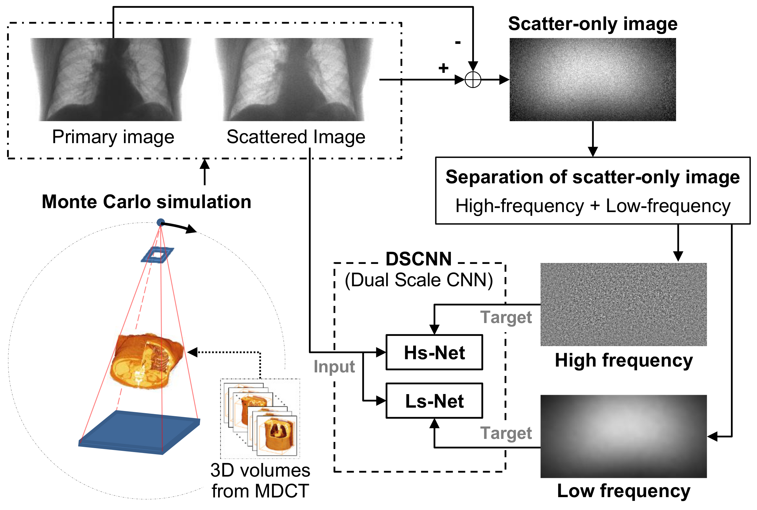
The training process of the proposed method is shown in Figure 1. In the figure, the 3D volume data from NBIA are used for generating synthetic X-ray images by MC simulation. As opposed to multi-detector CT (MDCT), the wide field of view (FOV) of CBCT for the human body can generate severe scattering, which degrades the image quality. Therefore, we chse a CBCT model for the simulation.
Through the simulation, we generated a set of image pairs composed of a scattered image and its corresponding scatter-free target image by increasing the dose amount. The synthetic image pairs were used firstly to train the CNN after the augmentation process in order to increase the amount of training data by the proper geometric transform and, secondly, to evaluate the performance of the trained network. The CNN in the proposed method was trained to estimate the difference between the scattered and scatter-free images, which corresponds to the scatter component in the input image that has been degraded by scatter.
We assumed that the scatter consists of low- and high-frequency components, and that the different types of the CNN structure effectively estimate each component separately. Once the two components were predicted in the separated branches of the CNN, they were combined to estimate the overall scatter. The scatter-free image was finally obtained by subtracting the overall scatter from the scattered input image.
2.1. Generation of Training and Test Images Based on MC Simulation
As aforementioned, CBCT was chosen as an example to generate the synthetic data for training the network. Because the spectra differ depending on the working systems, the simulation environment should be designed to resemble the real system and operating conditions as closely as possible. The specifications of CBCT for simulation are listed in Table 1. We set the tube voltage at 110 kV with a copper 0.2 mm filter, because it is a typical condition of CBCT.
To generate exceedingly many X-ray images from a large volume of 3D human body data, the speed of simulation is an important factor in choosing the simulation tool. Among the various available tools, we chose GATE [37,38] to support the GPU operation because it is reliable, convenient to use, and sufficiently versatile to make a proper and flexible model for CT. In the table, a relatively low resolution was taken to speed up the simulation process for synthetic data generation. However, the acquisition was sized as large as a real system in order to validate the proposed method.
The 3D volume data taken from MDCT, which contains little scatter compared to CBCT, were used to generate training and test images. The volume dataset was obtained from NBIA. Each volume dataset shows a patient’s real chest, which gives the anatomical variability of the human body. We took one and nine volumes of data to generate training and test images, respectively. During the MC simulation process, the gantry, composed of an X-ray generator and a detector, was rotated 360 degrees, and a pair of scattered and scatter-free images was obtained for every degree, which generated 360 pairs of images for the volume data. In addition, to increase the amount of data, each pair of images was rotated 180 degrees, and flipped horizontally and vertically, so that 4 × 360 pairs of images for a volume were produced, including the original pairs of images. The nine volumes give a total of 12,960 (4 after augmentation × 360 degrees × 9 volumes) X-ray image pairs for training. The size of image corresponds to the detector resolution, i.e., 256 × 128. The scattered X-ray image was generated in such a way that 5000 photons on average were captured at a pixel, which means 163,840,000 photons were considered in the simulation for a projected image. For the scatter-free image, the number of photons for a pixel was increased to 6000 so that 196,608,000 photons were considered for an image. In other words, the high-dosed projected image over 20% of the low-dosed one was treated as a scatter-free target. The pairs of scattered and scatter-free images were used in the training and testing of the proposed network. In the training, the scattered image was input into the network and its scatter-free image became the ultimate target to be achieved.
For testing the trained network, 360 (no augmentation, 360 degrees × 1 volume) pairs of scattered and scatter-free images from a volume were generated by the same simulation process. In the test, the augmentation to increase the data by rotation and flipping was meaningless, because it was not necessary to increase the number of data. In the test process, the scattered image was input into the trained network, and the scatter-free image was used to evaluate the performance by comparing it with the output of the network.
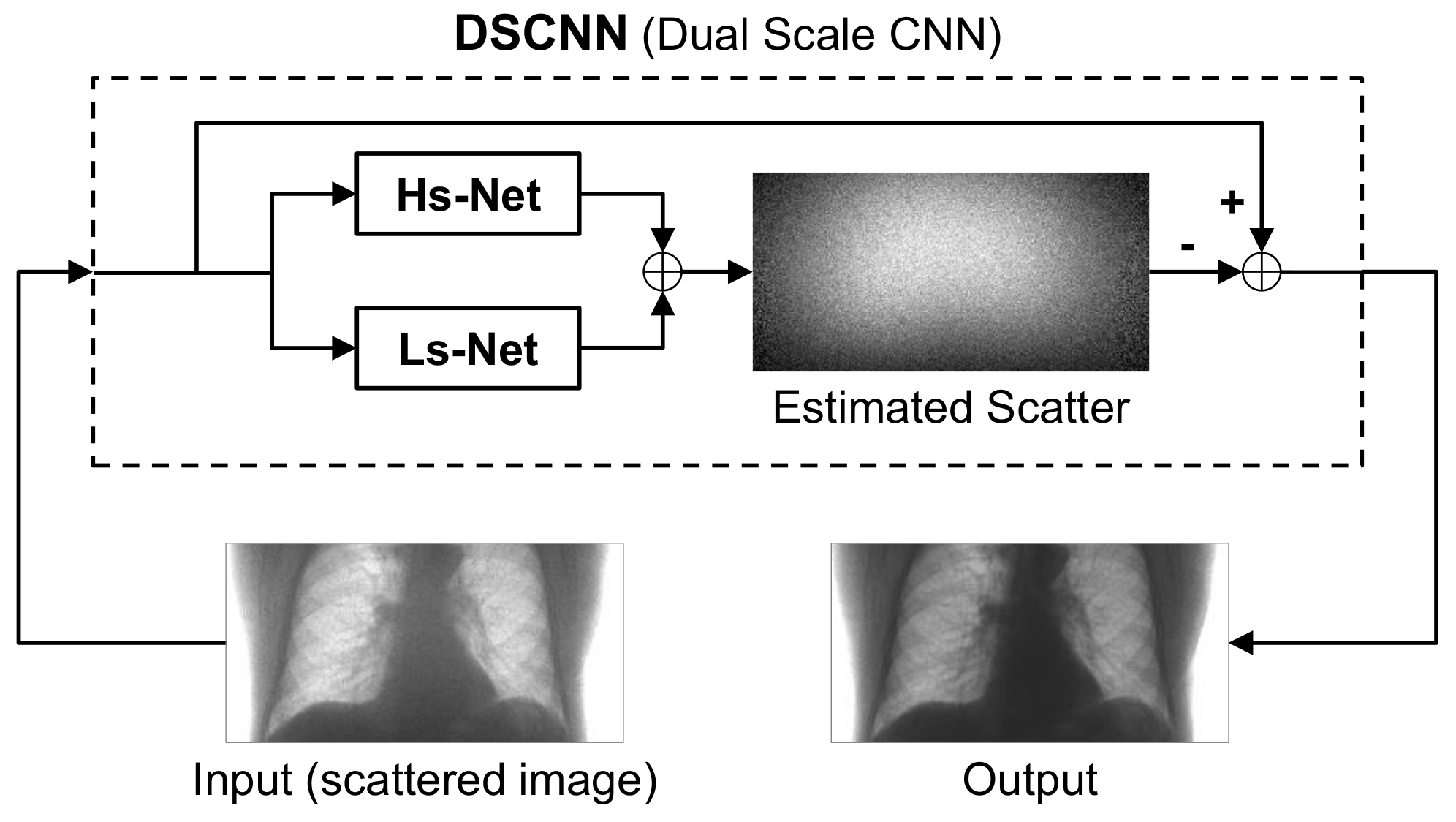
2.2. CNN-Based Scatter Correction
The CNN-based scatter correction was achieved by using a dual-scale CNN (DSCNN), as shown in Figure 2. The input into the network was a scattered X-ray image and the scatter component of the image was predicted by the trained network. To obtain a scatter-free image, the scatter component predicted by the network was subtracted from the input scattered image.
The DSCNN consists of two separate branches, Hs-Net and Ls-Net, which were designed to estimate the high- and low-frequency components of scatter, respectively. The two components were separately predicted in the parallel branches, and then combined to obtain the overall scatter.
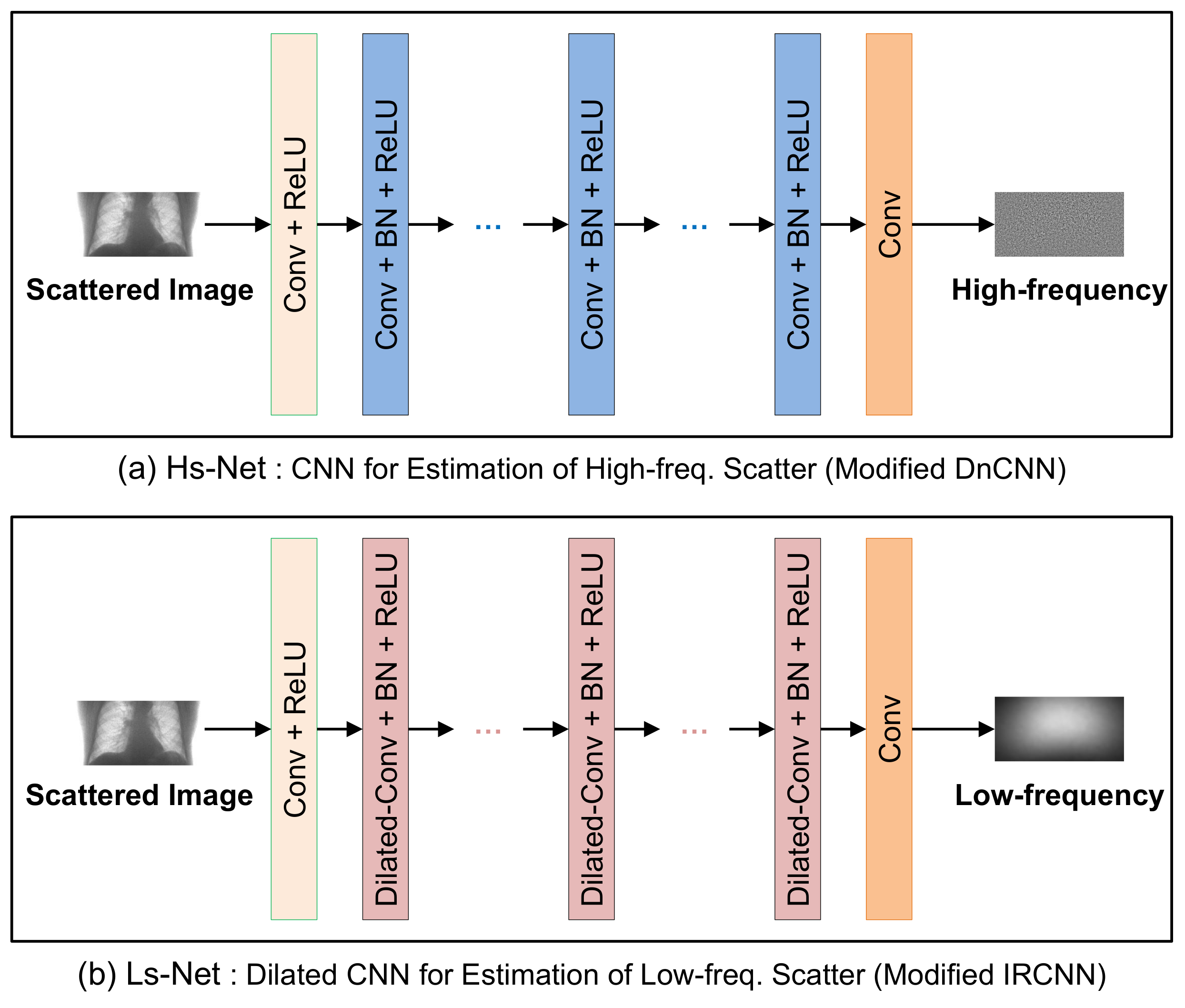
The Hs-Net and Ls-Net based on CNN are shown in Figure 3a,b, respectively. Hs-Net was inspired by DnCNN [17], in which successive CNN blocks are used to estimate the residual noise. The initial CNN block with BN is followed by CNN blocks, each of which has a BN and an ReLU activation function. Finally, a CNN block produces the residual of high-frequency scatter. Table 2a presents the size of the convolution filters and the number of filters in each layer with the corresponding receptive fields. As the network deepens, the spatial region of influence of a filter, called the receptive field, widens.
In Ls-Net for the low-frequency scatter, the dilated CNN was adopted instead of conventional CNN in order to expand the receptive field without increasing the number of weights as IRCNN [18]. The dilation rates, given in Table 2b, increase exponentially up to Layer 6, and then decrease at the same rate. The receptive field amounts to almost the same size of input image. The dilated convolution in Ls-Net is applied for capturing the wide-range variation of scattering over the whole region of images.
The input scattered image to the network is represented by , where p and s denote the target scatter-free image and the scatter-only image, respectively. The residual component of scatter, , was estimated by the network so that the scatter-corrected image can be obtained by .
The training of the network was performed to minimize the loss function
where , and are the loss of Hs-Net and Ls-Net adjustable with (usually set to 0.5), respectively, which are defined by
and
In the equations, and are the targets of the high- and low-frequency components for the ith input , respectively. The is the Gaussian smoothed scatter component by taking Gaussian low-pass filter on the scatter component of the ith input image, i.e. , where the size of window is 21 × 21 with . Once we calculated using the training data from MC simulation of nine volumes, the objective function in Equation (1) was minimized with respect to the network parameters , which correspond to the weights of the convolution filters. After training the parameters, the network estimated for scattered input , where and are the predicted high- and low-frequency components of scatter, respectively. Then, the scatter-corrected image can be obtained by .
2.3. Metrics for Performance Evaluation
We chose the three metrics, RMSE, PSNR, and SSIM, for objective performance evaluation, which are defined by
and
respectively.
3. Experimental Results and Discussion
In the experiment, we used a desktop PC with Intel Core i7 CPU and NVIDIA GeForce GTX 1060 GPU. From the MC simulation of nine volumes and three types of transform for data augmentation, 12,960 pairs of scattered and primary scatter-free images were obtained for training. In addition, 360 pairs from the same MC simulation of a volume without augmentation were obtained for testing and evaluation. It took about 18.71 days to generate the training set and test data with the three aforementioned desktop PCs.
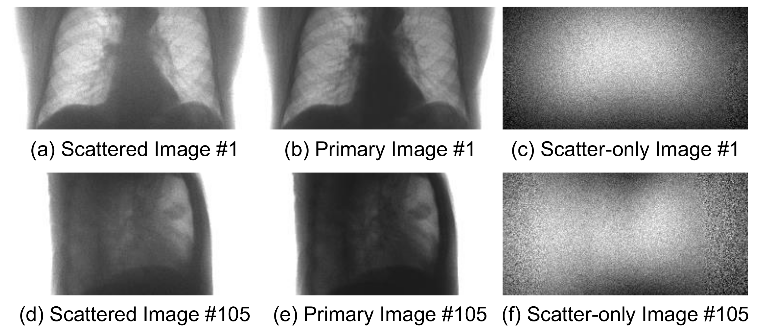
Figure 4 shows the sample pairs of projected images, in which each pair consists of the scattered image and the scatter-free primary image. The last column of the figure shows the residual images, which correspond to scatter components.
3.1. Network Training
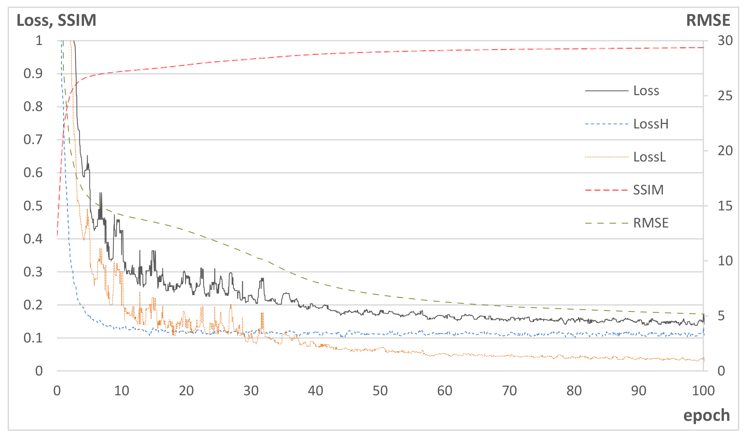
In the training, it took 13.3 days for 500 epochs in the aforementioned PC equipped with GPU. The batch size was 5 and all the batches were randomly reordered for every epoch. In an epoch, 12,960 pairs of training images were shown to the network to estimate the loss using Equation (1). The learning rate was initially set to , and scheduled to decrease to , and then set to the fixed value after 100 epochs. Adam optimizer [39] was taken to minimize the loss in Equation (1) with respect to weights of the network.
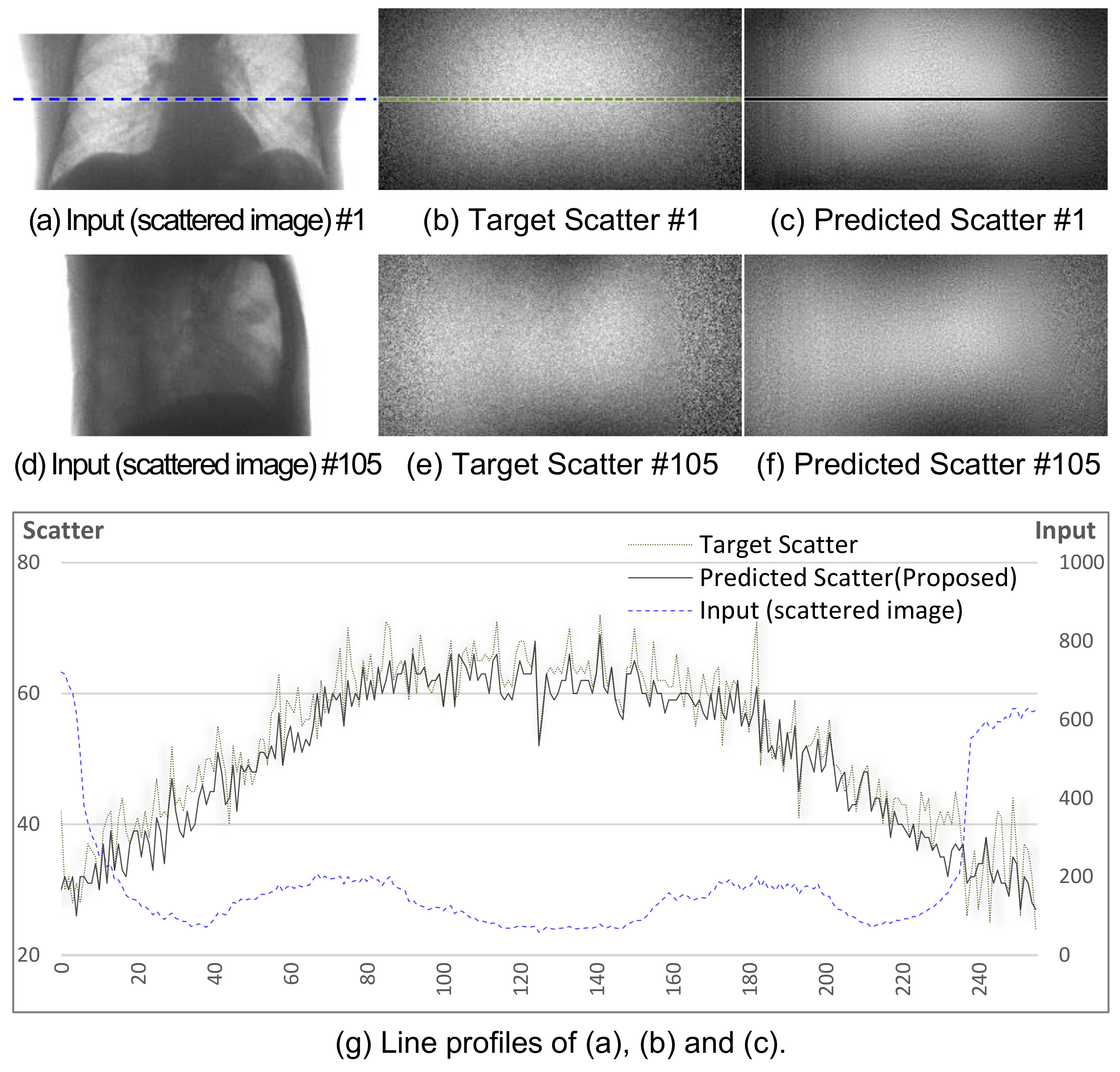
Figure 5 shows the learning curves of the training, where the losses were calculated from the training data, while RMSE and SSIM were obtained from test data. In the figure, SSIM increases as decreases, while RMSE decreases as decreases. This implies that Hs-Net contributes to the increase in the structural similarity by correcting the high-frequency component of scatter, while Ls-Net corrects the wide range of spatial scatter pattern over the entire image region. Figure 6a–f shows the two sets of sample images denoted by #1 and #105 after training. Figure 6g shows the profile of a specific row in the #1 image. The trained network generates similar scatter patterns to the corresponding targets.
3.2. Performance Evaluation with Comparison
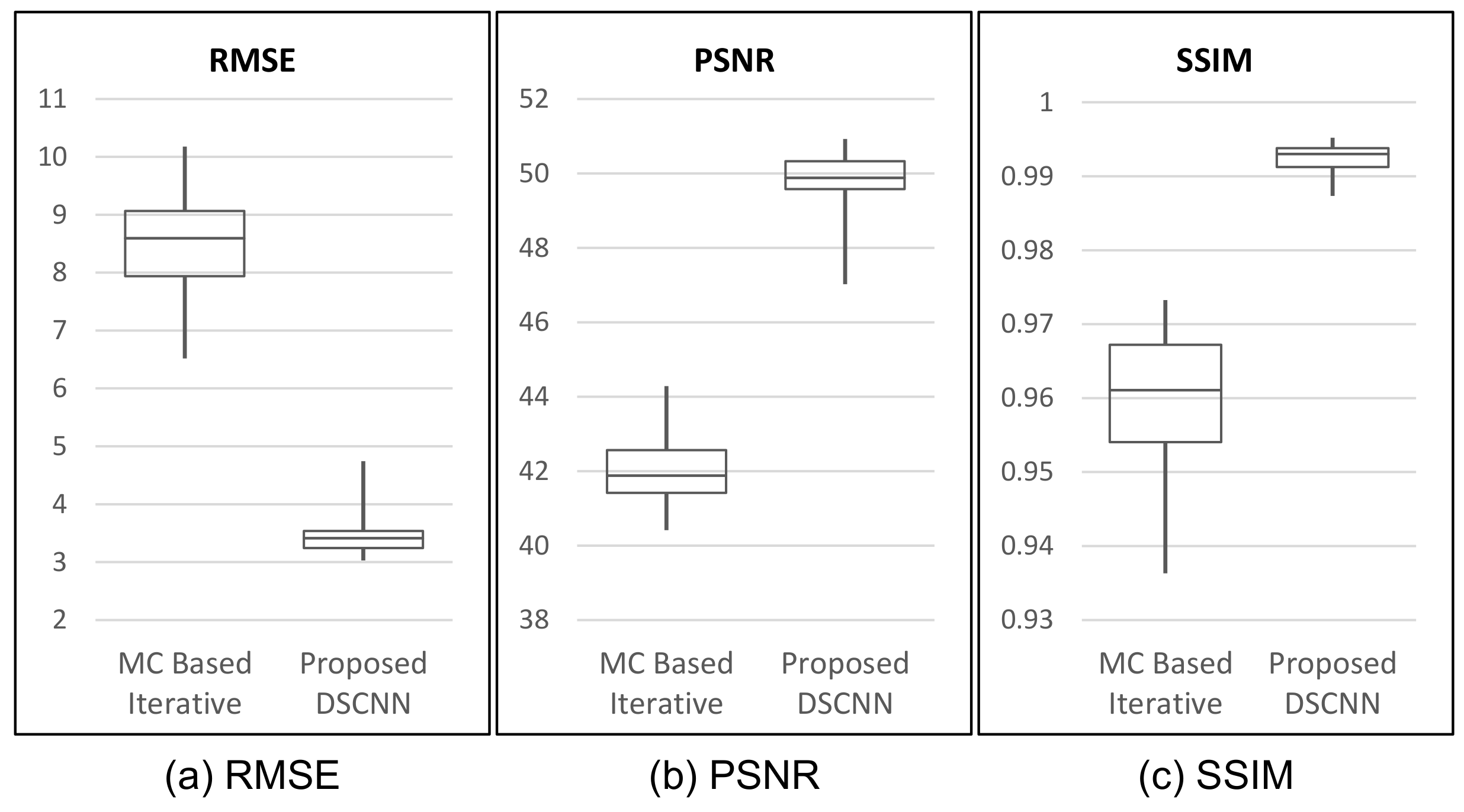
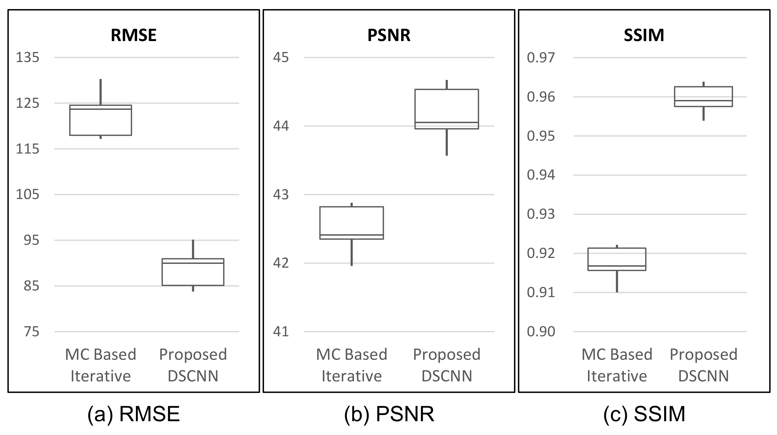
The set of 360 projected images from the MC simulation of a test volume, which is excluded from the training process, was used to evaluate the performance of the trained network for scatter correction. In the test, the correction of each scattered image took an average of 17.3 ms in the same PC set-up as that used in the training process. After the scatter correction by the proposed method, the RMSE, PSNR, and SSIM indices were calculated by comparison with its primary target image. Then, the average score and variance over all 360 images for each index were taken, as listed in Table 3. We compared the proposed method with the MC-based iterative scatter correction [10]. In the iterative method, we performed the MC simulation in such a way that 1000 photons on average were collected per pixel, which amounted to 32,768,000 photons for an image size of 256 × 128. The iteration algorithm was stopped if the difference in average RMSE over the slices at the center of the 3D reconstructed volume between consecutive iterations was less than 0.001 cm−1. Five iterations were performed, which took over about five days for all 360 images.
In Table 3, our proposed method shows superior performance to that of the MC-based iterative one with respect to all three indices of performance evaluation. The proposed method shows better results, with as much as 58.5% reduction in RMSE, and 18.1% and 3.4% increases in PSNR and SSIM, on average, respectively. The box-whiskers plot in Figure 7 shows that the proposed method produces a more stable result than the MC-based iterative one does.
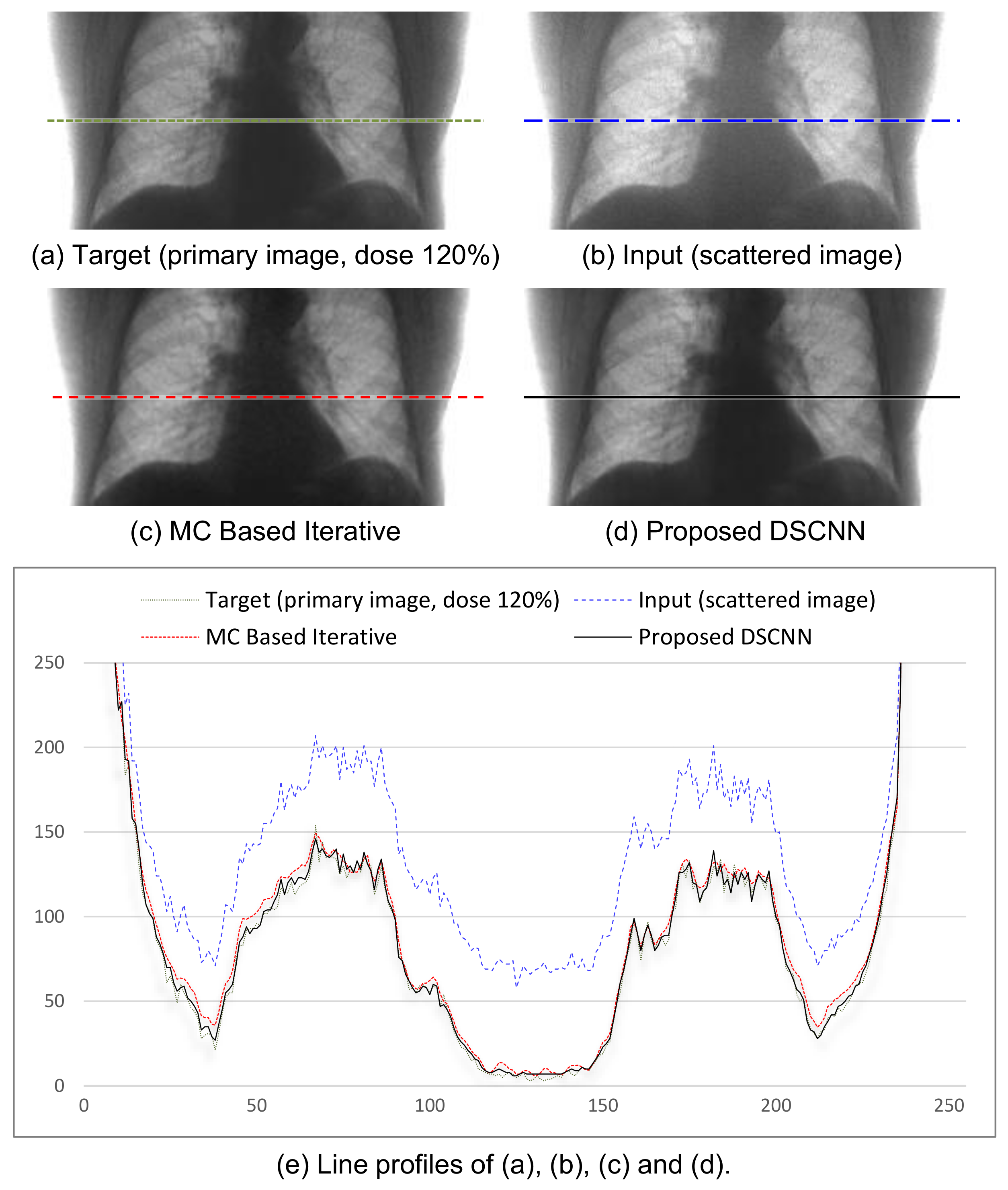
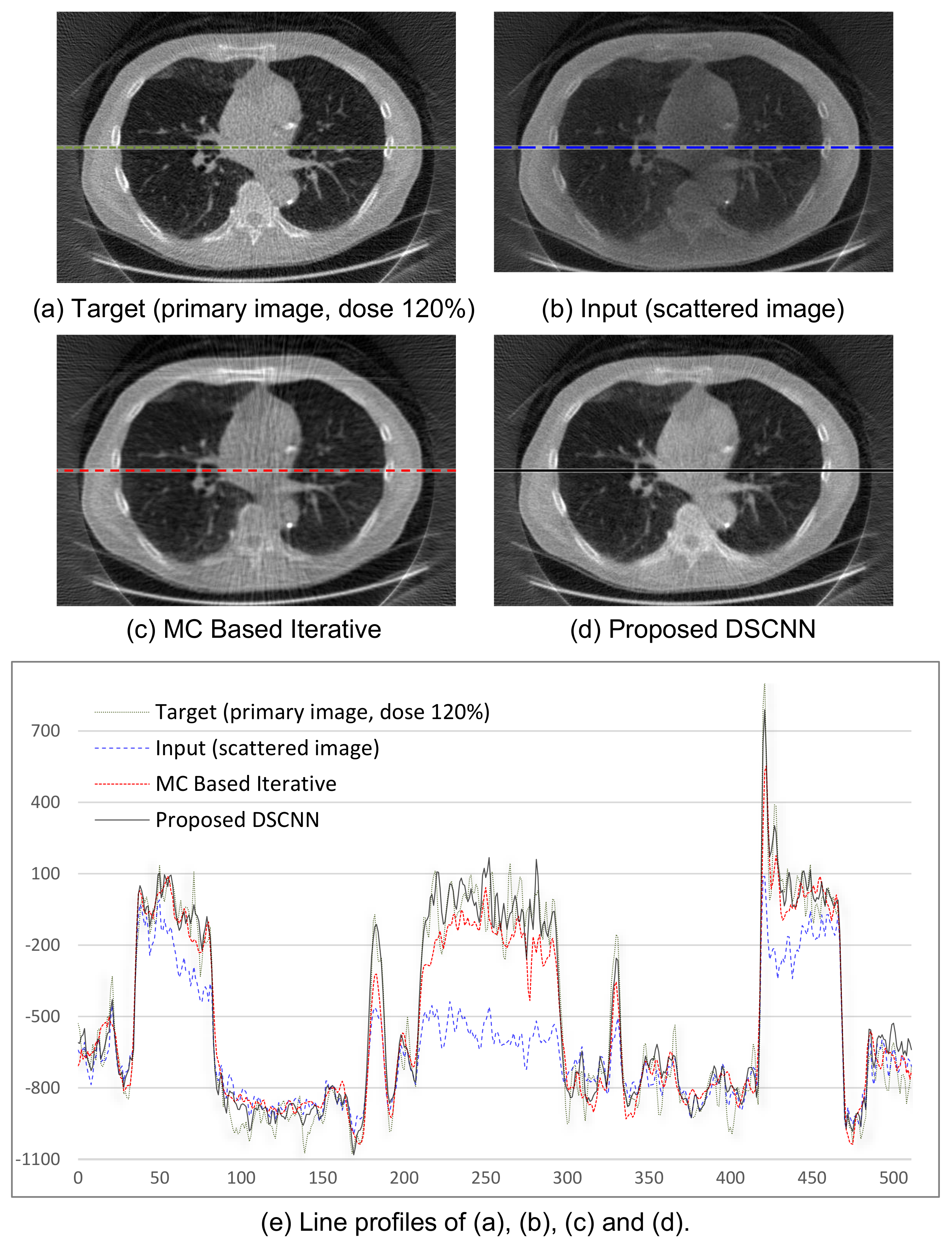
The average SSIM of 0.992 in Table 3 indicates that the proposed method can produce the scatter correction with high structural similarity with small variance. This is a required property of scatter correction, because a result with less scatter could provide additional artifacts or lose important information for medical diagnosis. Figure 8a–d shows the visual results of the two correction methods, and Figure 8e the line profiles of the four images in Figure 8a–d. Again, the proposed method predicts the target images more accurately than the MC-based one.
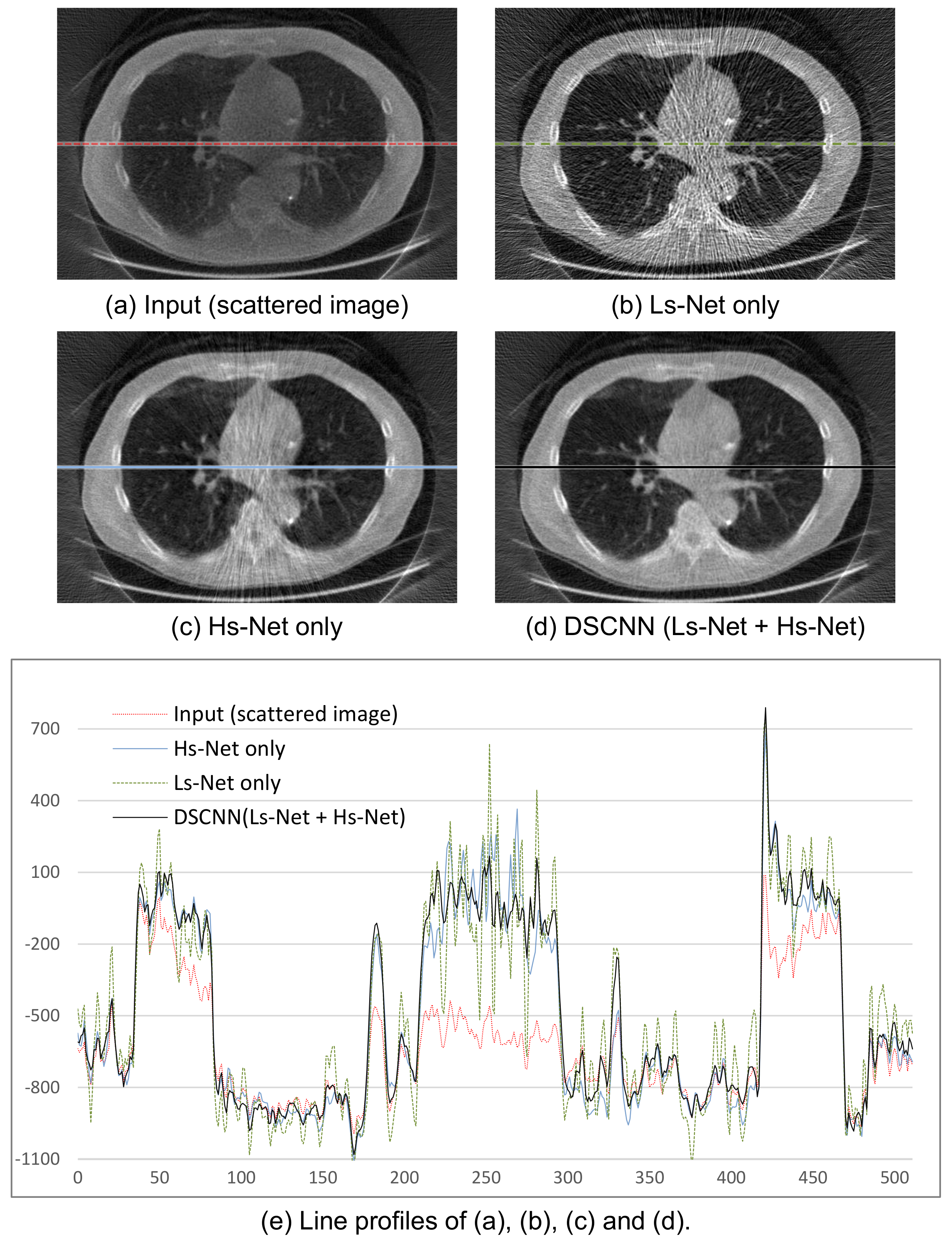
The performances of the 3D reconstructed image after scatter correction are shown in Figure 9. The images in Figure 9b–d were obtained from the separately trained Ls-Net and Hs-Net, and from the combined Ls- and Hs-Net, respectively. Figure 9b shows that a single branch of Ls-Net enhances the overall contrast of the image by compensating for the low-frequency scatter component, but generates streak artifacts due to high-frequency component of scatter and noise. Meanwhile, Figure 9c shows that a single branch of Hs-Net reduces the streak artifacts, but the corresponding profile in Figure 9e reveals the uniformity of the image is not so good. Further, relatively numerous artifacts are visibly, especially on the pathway of the X-ray beam going through thick and dense objects where severe scatter occurs. In summary, Ls-Net is suitable for correcting the low-frequency scatter component, but not the high-frequency component. Therefore, the dual-branch structure, where Hs-Net complements Ls-Net, effectively provides scatter correction, as shown in Figure 9d. Figure 9e shows the profile images of a specific line of the resulting images.
In Table 4, the performance of the proposed DSCNN after 3D reconstruction is compared with that of the MC-based iteration method. We record the average scores over the slices at the center of 3D volumes of the reconstructed images after scatter correction and of the scatter-less target. For all three indices, the proposed DSCNN outperforms the MC-based iteration method. The proposed method produces a 27.6% reduction in RMSE, and 4.0% and 4.6% increases in PSNR and SSIM, respectively, on average, compared to the MC-based one. Figure 10 shows the box-whiskers plot, which demonstrates that the proposed method produces more or less stable results.
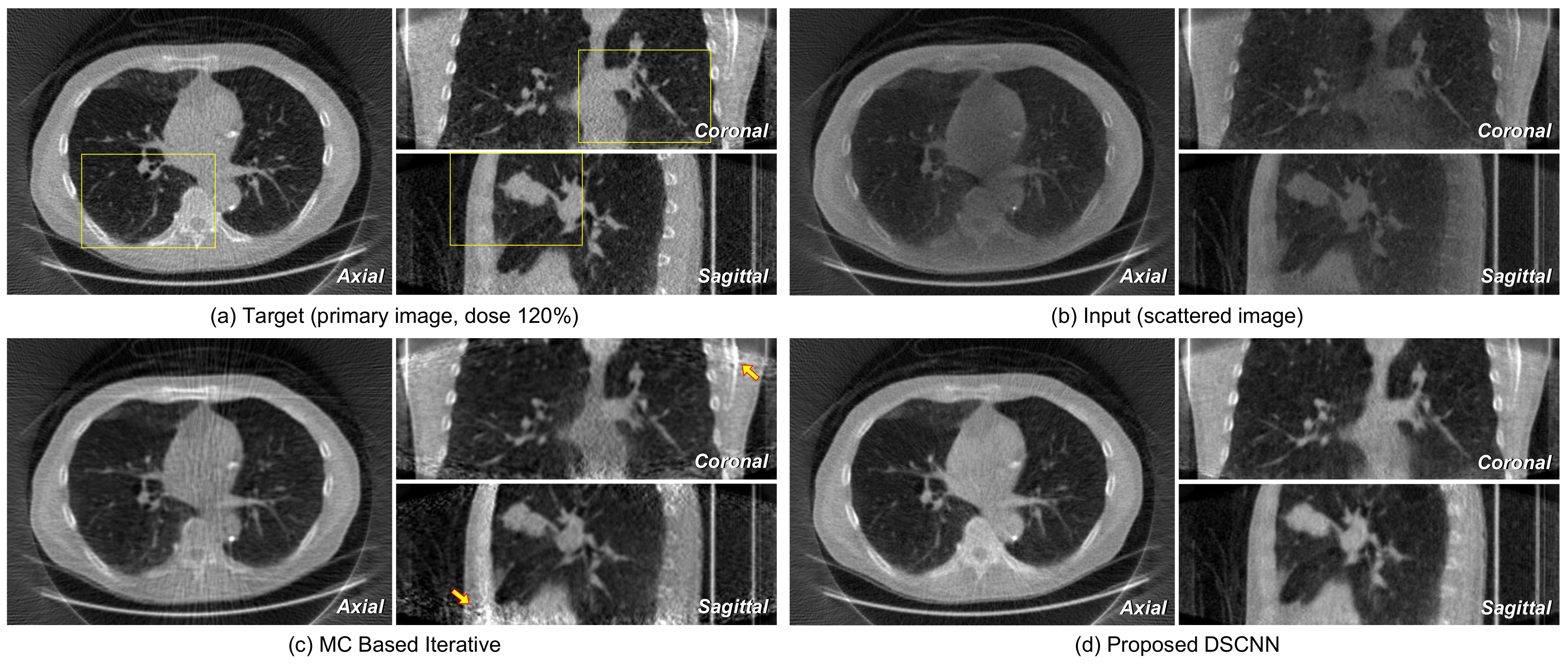
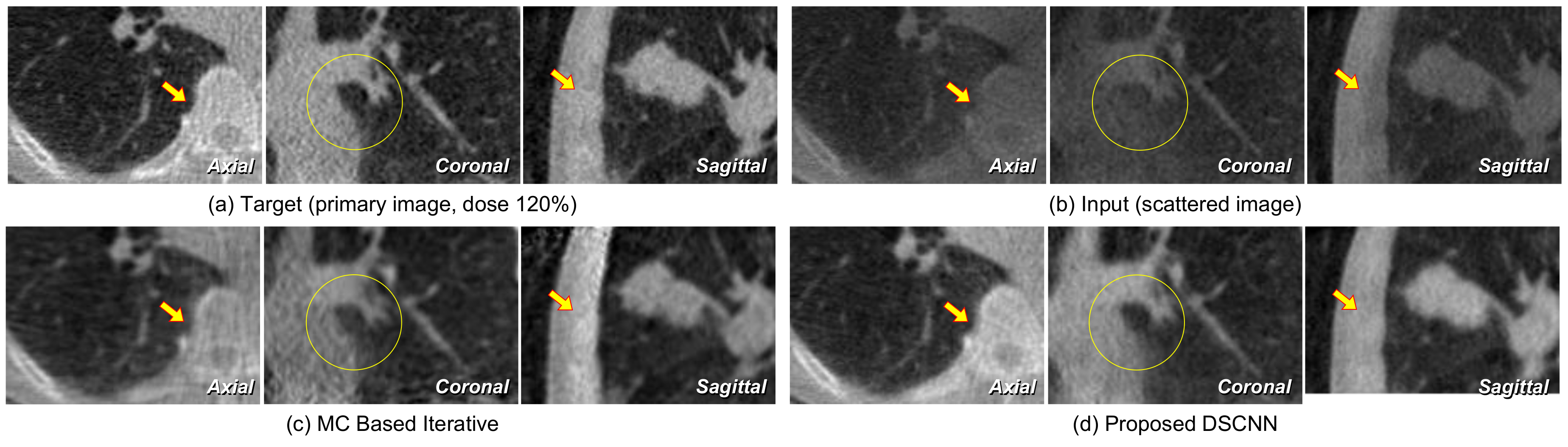
Figure 11 shows the axial images taken from reconstructed volumes with specific profile data. The superiority of the proposed DSCNN against MC-based method is evident from both the sliced image and the profile. Figure 12a,b represents the axial, coronal, and sagittal images of a target and its corresponding input scattered image, respectively. Figure 12c shows that no additional artifact is generated from the proposed DSCNN, as opposed to the MC-based iteration method in Figure 12d. However, additional artifacts are seen in the coronal and sagittal images at the arrow-indicted parts of the images from the MC-based iteration method. The regions enclosed by the yellow rectangles in Figure 12 are magnified in Figure 13. The proposed DSCNN enhances the bone boundary in the axial image (arrow), recovers the morphological information in the coronal image (circle), and well reveals the shading in soft structure in the sagittal image (arrow). The MC-based iterative method produces additional noise in the soft structure.
4. Conclusions
Conventional strategies for scatter reduction based on physical equipment or measurements inevitably increase the dose to improve the image quality. In addition, scatter reduction based on a computational algorithm requires an accurate model for the complicated degradation process, or it could take a large amount time for iterative MC simulation.
This paper proposes a CNN-based scatter correction method. In general, this type of deep learning approach requires a large amount of training data. Because of the difficulty in obtaining such a training dataset in the real world, MC simulation is performed to generate the data off-line in the proposed method. The CBCT is so vulnerable to scatter that we apply it in the present study with the aim of demonstrating clear improvement, even though our proposed method can be generally applied to projected X-ray images. After obtaining synthetic data that are sufficiently similar so as to be treated as real data by MC simulation, they can be used for training the CNN for image restoration, after which the CNN can be used for scatter correction of X-ray images.
In the method, the CNN architecture consists of two parallel branches to estimate scattering: one for the high- and the other for the low-frequency component. For the low-frequency branch, the dilated convolution filters are adapted to increase the receptive field to estimate the slowly varying scatter components over the entire image. For the high-frequency branch, only convolution filters are used to estimate the fast varying scatter. Then, the estimated high- and low-frequency components of scatter can be combined, and finally subtracted from the input scattered image to produce a scatter-corrected output image.
In the experiment, the training dataset was obtained from an MC simulation of real chest CT volume data of NBIA and augmented to increase the number of data. Again, a test dataset from the MC simulation of a test volume was used to evaluate the performance of the trained network.
The RMSE, PSNR, and SSIM indices were calculated, and the average scores over all test images for each index were taken, along with their variances. Even though the test was performed on synthetic data, the quantitative evaluation results for both 2D image and 3D reconstructed volume data show that the proposed method is effective in terms of RMSE, PSNR and SSIM indices with increased stability. Compared with the MC-based iterative method, the proposed method produces better results, with as much as 58.5% reduction in RMSE, and 18.1% and 3.4% increases in PSNR and SSIM, respectively, on average, for the projected images, and 27.6% decrease in RMSE, and 4.0% and 4.6% enhancements in PSNR and SSIM, respectively, on average, for the reconstructed images. In addition, qualitative results show that the contrast can be well improved by the scatter correction without additional artifacts. The proposed scatter correction is so fast that it only takes about 17.3 ms for the correction of a projected image in a PC with GPU.
Because research on deep learning-based scatter correction has only recently commenced, we did not compare our results with those of other methods. However, we expect that various deep learning models will be developed for scatter correction, once a training dataset is obtained by the proposed simulation method.
In general, collecting synthetic data for MC simulation takes a long time, thus we only examined the chest region with low-resolution images. Furthermore, we validated our method by using the target scatter-free images with an increased dose of only 20%. We believe that the superior performance of proposed method renders it capable of being applied to real X-ray images if the training data are taken with increased resolution and dose amount in an improved, fast simulation environment close to that of real X-ray CT.
Author Contributions
Project administration, H.L.; Supervision, J.L.
Funding
This work was supported in part by Basic Science Research Program through the National Research Foundation of Korea (NRF) funded by the Ministry of Education (No. 2019R1A6A1A09031717) and Brain Korea 21 PLUS Project, National Research Foundation of Korea.
Conflicts of Interest
The authors declare no conflict of interest.
References
- Neitzel, U. Grids or air gaps for scatter reduction in digital radiography: A model calculation. Med. Phys. 1992, 19, 475–481. [Google Scholar] [CrossRef] [PubMed]
- Schafer, S.; Stayman, J.W.; Zbijewski, W.; Schmidgunst, C.; Kleinszig, G.; Siewerdsen, J.H. Antiscatter grids in mobile C-arm cone-beam CT: Effect on image quality and dose. Med. Phys. 2012, 39, 153–159. [Google Scholar] [CrossRef] [PubMed]
- Ning, R.; Tang, X.; Conover, D. X-ray scatter correction algorithm for cone beam CT imaging. Med. Phys. 2004, 31, 1195–1202. [Google Scholar] [CrossRef] [PubMed]
- Maltz, J.S.; Gangadharan, B.; Vidal, M.; Paidi, A.; Bose, S.; Faddegon, B.A.; Aubin, M.; Morin, O.; Pouliot, J.; Zheng, Z.; et al. Focused beam-stop array for the measurement of scatter in megavoltage portal and cone beam CT imaging. Med. Phys. 2008, 35, 2452–2462. [Google Scholar] [CrossRef] [PubMed]
- Ohnesorge, B.; Flohr, T.; Klingenbeck-Regn, K. Efficient object scatter correction algorithm for third and fourth generation CT scanners. Eur. Radiol. 1999, 9, 563–569. [Google Scholar] [CrossRef]
- Li, H.; Mohan, R.; Zhu, X.R. Scatter kernel estimation with an edge-spread function method for cone-beam computed tomography imaging. Phys. Med. Biol. 2008, 53, 6729. [Google Scholar] [CrossRef] [PubMed]
- Star-Lack, J.; Sun, M.; Kaestner, A.; Hassanein, R.; Virshup, G.; Berkus, T.; Oelhafen, M. Efficient scatter correction using asymmetric kernels. Medical Imaging 2009: Physics of Medical Imaging. Int. Soc. Opt. Photon. 2009, 7258, 72581Z. [Google Scholar]
- Jarry, G.; Graham, S.A.; Moseley, D.J.; Jaffray, D.J.; Siewerdsen, J.H.; Verhaegen, F. Characterization of scattered radiation in kV CBCT images using Monte Carlo simulations. Med. Phys. 2006, 33, 4320–4329. [Google Scholar] [CrossRef] [Green Version]
- Sun, M.; Star-Lack, J. Improved scatter correction using adaptive scatter kernel superposition. Phys. Med. Biol. 2010, 55, 6695. [Google Scholar] [CrossRef]
- Watson, P.G.; Mainegra-Hing, E.; Tomic, N.; Seuntjens, J. Implementation of an efficient Monte Carlo calculation for CBCT scatter correction: phantom study. J. Appl. Clin. Med. Phys. 2015, 16, 216–227. [Google Scholar] [CrossRef]
- Peplow, D.E.; Verghese, K. Digital mammography image simulation using Monte Carlo. Med. Phys. 2000, 27, 568–579. [Google Scholar] [CrossRef]
- Sisniega, A.; Zbijewski, W.; Badal, A.; Kyprianou, I.; Stayman, J.; Vaquero, J.J.; Siewerdsen, J. Monte Carlo study of the effects of system geometry and antiscatter grids on cone-beam CT scatter distributions. Med. Phys. 2013, 40, 051915. [Google Scholar] [CrossRef] [Green Version]
- Mainegra-Hing, E.; Kawrakow, I. Fast Monte Carlo calculation of scatter corrections for CBCT images. J. Phys. 2008, 102, 012017. [Google Scholar] [CrossRef]
- Mainegra-Hing, E.; Kawrakow, I. Variance reduction techniques for fast Monte Carlo CBCT scatter correction calculations. Phys. Med. Biol. 2010, 55, 4495. [Google Scholar] [CrossRef]
- Thing, R.S.; Bernchou, U.; Mainegra-Hing, E.; Brink, C. Patient-specific scatter correction in clinical cone beam computed tomography imaging made possible by the combination of Monte Carlo simulations and a ray tracing algorithm. Acta Oncol. 2013, 52, 1477–1483. [Google Scholar] [CrossRef] [Green Version]
- Thing, R.S.; Mainegra-Hing, E. Optimizing cone beam CT scatter estimation in egs_cbct for a clinical and virtual chest phantom. Med. Phys. 2014, 41, 071902. [Google Scholar] [CrossRef] [Green Version]
- Zhang, K.; Zuo, W.; Chen, Y.; Meng, D.; Zhang, L. Beyond a gaussian denoiser: Residual learning of deep cnn for image denoising. IEEE Trans. Image Process. 2017, 26, 3142–3155. [Google Scholar] [CrossRef]
- Zhang, K.; Zuo, W.; Gu, S.; Zhang, L. Learning deep CNN denoiser prior for image restoration. In Proceedings of the IEEE Conference on Computer Vision and Pattern Recognition, Honolulu, HI, USA, 21–26 July 2017; Volume 2. [Google Scholar]
- Xu, L.; Ren, J.S.; Liu, C.; Jia, J. Deep convolutional neural network for image deconvolution. In Proceedings of the Advances in Neural Information Processing Systems, Montreal, QC, Canada, 8–13 December 2014; pp. 1790–1798. [Google Scholar]
- Chakrabarti, A. A neural approach to blind motion deblurring. In Proceedings of the European Conference on Computer Vision, Amsterdam, The Netherlands, 8–16 October 2016; pp. 221–235. [Google Scholar]
- Nah, S.; Kim, T.H.; Lee, K.M. Deep multi-scale convolutional neural network for dynamic scene deblurring. In Proceedings of the CVPR, Honolulu, HI, USA, 21–26 July 2017; Volume 1, p. 3. [Google Scholar]
- Chen, H.; Zhang, Y.; Kalra, M.K.; Lin, F.; Chen, Y.; Liao, P.; Zhou, J.; Wang, G. Low-dose CT with a residual encoder-decoder convolutional neural network. IEEE Trans. Med. Imaging 2017, 36, 2524–2535. [Google Scholar] [CrossRef]
- Simonyan, K.; Zisserman, A. Very deep convolutional networks for large-scale image recognition. arXiv 2014, arXiv:1409.1556. [Google Scholar]
- Krizhevsky, A.; Sutskever, I.; Hinton, G.E. Imagenet classification with deep convolutional neural networks. In Advances in Neural Information Processing Systems; MIT Press Ltd.: Cambridge, MA, USA, 2012; pp. 1097–1105. [Google Scholar]
- Ioffe, S.; Szegedy, C. Batch normalization: Accelerating deep network training by reducing internal covariate shift. arXiv 2015, arXiv:1502.03167. [Google Scholar]
- He, K.; Zhang, X.; Ren, S.; Sun, J. Deep residual learning for image recognition. In Proceedings of the IEEE Conference on Computer Vision and Pattern Recognition, Las Vegas, NV, USA, 27–30 June 2016; pp. 770–778. [Google Scholar]
- Yu, F.; Koltun, V. Multi-scale context aggregation by dilated convolutions. arXiv 2015, arXiv:1511.07122. [Google Scholar]
- Chen, L.C.; Papandreou, G.; Kokkinos, I.; Murphy, K.; Yuille, A.L. Deeplab: Semantic image segmentation with deep convolutional nets, atrous convolution, and fully connected crfs. IEEE Trans. Pattern Anal. Mach. Intell. 2018, 40, 834–848. [Google Scholar] [CrossRef]
- Yu, F.; Koltun, V.; Funkhouser, T. Dilated residual networks. In Proceedings of the Computer Vision and Pattern Recognition, Honolulu, HI, USA, 21–26 July 2017; Volume 1, p. 2. [Google Scholar]
- Wang, T.; Sun, M.; Hu, K. Dilated Deep Residual Network for Image Denoising. In Proceedings of the 2017 IEEE 29th International Conference on Tools with Artificial Intelligence (ICTAI), Boston, MA, USA, 6–8 November 2017; pp. 1272–1279. [Google Scholar]
- Liu, W.; Lee, J. An Efficient Residual Learning Neural Network for Hyperspectral Image Superresolution. IEEE J. Sel. Top. Appl. Earth Obs. Remote Sens. 2019, 12, 1240–1253. [Google Scholar] [CrossRef]
- Kang, E.; Min, J.; Ye, J.C. A deep convolutional neural network using directional wavelets for low-dose X-ray CT reconstruction. Med. Phys. 2017, 44, e360–e375. [Google Scholar] [CrossRef] [Green Version]
- Xu, S.; Prinsen, P.; Wiegert, J.; Manjeshwar, R. Deep residual learning in CT physics: scatter correction for spectral CT. arXiv 2017, arXiv:1708.04151. [Google Scholar]
- Hansen, D.C.; Landry, G.; Kamp, F.; Li, M.; Belka, C.; Parodi, K.; Kurz, C. ScatterNet: A convolutional neural network for cone-beam CT intensity correction. Med. Phys. 2018, 45, 4916–4926. [Google Scholar] [CrossRef]
- Yang, J.; Park, D.; Gullberg, G.T.; Seo, Y. Joint correction of attenuation and scatter in image space using deep convolutional neural networks for dedicated brain 18F-FDG PET. Phys. Med. Biol. 2019, 64, 075019. [Google Scholar] [CrossRef]
- National Cancer Institute. NBIA—National Biomedical Imaging Archive. Available online: https://imaging.nci.nih.gov/ (accessed on 9 June 2017).
- Jan, S.; Santin, G.; Strul, D.; Staelens, S.; Assie, K.; Autret, D.; Avner, S.; Barbier, R.; Bardies, M.; Bloomfield, P.; et al. GATE: A simulation toolkit for PET and SPECT. Phys. Med. Biol. 2004, 49, 4543. [Google Scholar] [CrossRef]
- Jan, S.; Benoit, D.; Becheva, E.; Carlier, T.; Cassol, F.; Descourt, P.; Frisson, T.; Grevillot, L.; Guigues, L.; Maigne, L.; et al. GATE V6: A major enhancement of the GATE simulation platform enabling modelling of CT and radiotherapy. Phys. Med. Biol. 2011, 56, 881. [Google Scholar] [CrossRef]
- Kingma, D.P.; Ba, J. Adam: A method for stochastic optimization. arXiv 2014, arXiv:1412.6980. [Google Scholar]
- The Startling Power of Synthetic Data—Towards Data Science. Available online: https://towardsdatascience.com/the-startling-power-of-synthetic-data-604aadb78c9d (accessed on 19 August 2019).
- Tremblay, J.; Prakash, A.; Acuna, D.; Brophy, M.; Jampani, V.; Anil, C.; To, T.; Cameracci, E.; Boochoon, S.; Birchfield, S. Training deep networks with synthetic data: Bridging the reality gap by domain randomization. In Proceedings of the IEEE Conference on Computer Vision and Pattern Recognition Workshops, Munich, Germany, 8–14 September 2018; pp. 969–977. [Google Scholar]
Figure 1.
Training process of the proposed scatter correction method.

Figure 2.
Test process of the proposed scatter correction method.

Figure 3.
Hs-Net for high-frequency component of scatter (a); and Ls-Net for low-frequency component of scatter (b).
Figure 3.
Hs-Net for high-frequency component of scatter (a); and Ls-Net for low-frequency component of scatter (b).

Figure 4.
Examples of pairs of scattered and scatter-free primary images with their residuals.

Figure 5.
Learning curves of training (losses for training data, SSIM and RMSE for test data).

Figure 6.
Predicted scatter after training.

Figure 7.
Box and whiskers plots of Table 3.
Figure 7.
Box and whiskers plots of Table 3.

Figure 8.
Comparison of scatter-corrected images and line profiles.

Figure 9.
Performance of reconstructed images after scatter correction.

Figure 10.
Box and whiskers plots of Table 4.
Figure 10.
Box and whiskers plots of Table 4.

Figure 11.
Comparison of axial images after reconstruction and the line profiles.

Figure 12.
Comparison of 3D reconstructed images: target primary image (a); input scattered image (b); and after scatter correction (c,d).
Figure 12.
Comparison of 3D reconstructed images: target primary image (a); input scattered image (b); and after scatter correction (c,d).

Figure 13.
Magnified images of the yellow rectangle regions in Figure 12.
Figure 13.
Magnified images of the yellow rectangle regions in Figure 12.


Table 1.
Specification of CBCT for Simulation.
| Item | Specification of CBCT |
|---|---|
| SDD (mm) | 685 |
| SOD (mm) | 400 |
| FOV (x,y,z) (mm) | 358 × 358 × 200 |
| X-ray Tube kV | 110 kV |
| X-ray Filter | Cu 0.2 mm |
| X-ray Detector Size (mm) | 686 × 343 |
| X-ray Detector Resolution (pixel) | 256 × 128 |
| 3D Object Size (x,y,z) (mm) | 400 × 400 × 300 |
Table 2.
Network specifications of Hs-Net and Ls-Net.
| (a) Hs-Net: CNN for Estimation of High-Frequency Scatter (Modified DnCNN [17]) | ||||||||||||
| Layer | 1 | 2 | 3 | 4 | 5 | 6 | 7 | 8 | 9 | 10 | 11 | 12 |
| Convolution | 3 × 3 × 1 | 3 × 3 × 64 | 3 × 3 × 64 | 3 × 3 × 64 | 3 × 3 × 64 | 3 × 3 × 64 | 3 × 3 × 64 | 3 × 3 × 64 | 3 × 3 × 64 | 3 × 3 × 64 | 3 × 3 × 64 | 3 × 3 × 64 |
| Receptive field | 3 × 3 | 5 × 5 | 7 × 7 | 9 × 9 | 11 × 11 | 13 × 13 | 15 × 15 | 17 × 17 | 19 × 19 | 21 × 21 | 23 × 23 | 25 × 25 |
| Output channels | 64 | 64 | 64 | 64 | 64 | 64 | 64 | 64 | 64 | 64 | 64 | 1 |
| (b) Ls-Net: Dilated CNN for Estimation of Low-Frequency Scatter (Modified IRCNN [18]) | ||||||||||||
| Layer | 1 | 2 | 3 | 4 | 5 | 6 | 7 | 8 | 9 | 10 | 11 | 12 |
| Convolution | 3 × 3 × 1 | 3 × 3 × 64 | 3 × 3 × 64 | 3 × 3 × 64 | 3 × 3 × 64 | 3 × 3 × 64 | 3 × 3 × 64 | 3 × 3 × 64 | 3 × 3 × 64 | 3 × 3 × 64 | 3 × 3 × 64 | 3 × 3 × 64 |
| Dilation rate | 1 | 2 | 4 | 8 | 16 | 32 | 32 | 16 | 8 | 4 | 2 | 1 |
| Receptive field | 3 × 3 | 7 × 7 | 15 × 15 | 31 × 31 | 63 × 63 | 127 × 127 | 191 × 191 | 223 × 223 | 239 × 239 | 247 × 247 | 251 × 251 | 253 × 253 |
| Output channels | 64 | 64 | 64 | 64 | 64 | 64 | 64 | 64 | 64 | 64 | 64 | 1 |
Table 3.
Comparison of projected images after scatter correction.
| Index | MC Based Iterative | Proposed DSCNN | ||
|---|---|---|---|---|
| Average | Variance | Average | Variance | |
| RMSE | 8.43 | 0.829 | 3.50 | 0.151 |
| PSNR | 42.10 | 0.959 | 49.72 | 0.787 |
| SSIM | 0.960 | 8.5 × | 0.992 | 4.5 × |
Table 4.
Comparison of reconstructed images after scatter correction.
| Index | MC Based Iterative | Proposed DSCNN | ||
|---|---|---|---|---|
| Average | Variance | Average | Variance | |
| RMSE | 122.11 | 15.948 | 88.41 | 13.176 |
| PSNR | 42.53 | 0.080 | 44.21 | 0.127 |
| SSIM | 0.918 | 1.2 × | 0.960 | 9.8 × |
© 2019 by the authors. Licensee MDPI, Basel, Switzerland. This article is an open access article distributed under the terms and conditions of the Creative Commons Attribution (CC BY) license (http://creativecommons.org/licenses/by/4.0/).
Share and Cite
MDPI and ACS Style
Lee, H.; Lee, J. A Deep Learning-Based Scatter Correction of Simulated X-ray Images. Electronics 2019, 8, 944. https://doi.org/10.3390/electronics8090944
AMA Style
Lee H, Lee J. A Deep Learning-Based Scatter Correction of Simulated X-ray Images. Electronics. 2019; 8(9):944. https://doi.org/10.3390/electronics8090944
Chicago/Turabian StyleLee, Heesin, and Joonwhoan Lee. 2019. "A Deep Learning-Based Scatter Correction of Simulated X-ray Images" Electronics 8, no. 9: 944. https://doi.org/10.3390/electronics8090944
Note that from the first issue of 2016, this journal uses article numbers instead of page numbers. See further details here.