A Traffic Flow Prediction Method Based on Road Crossing Vector Coding and a Bidirectional Recursive Neural Network


School of Mechanical Engineering, Xi’an University of Science and Technology, Xi’an 710054, China
*
Author to whom correspondence should be addressed.
Electronics 2019, 8(9), 1006; https://doi.org/10.3390/electronics8091006
Submission received: 17 August 2019
/
Revised: 5 September 2019
/
Accepted: 5 September 2019
/
Published: 8 September 2019
(This article belongs to the Special Issue Intelligent Transportation Systems (ITS))
Abstract
:Aiming at the problems that current predicting models are incapable of extracting the inner rule of the traffic flow sequence in traffic big data, and unable to make full use of the spatio-temporal relationship of the traffic flow to improve the accuracy of prediction, a Bi-directional Regression Neural Network (BRNN) is proposed in this paper, which can fully apply the context information of road intersections both in the past and the future to predict the traffic volume, and further to make up the deficiency that the current models can only predict the next-moment output according to the time series information in the previous moment. Meanwhile, a vectorized code to screen out the intersections related to the predicting point in the road network and to train and predict through inputting the track data of the selected intersections into BRNN, is designed. In addition, the model is testified through the true traffic data in partial area of Shen Zhen. The results indicate that, compared with current traffic predicting models, the model in this paper is capable of providing the necessary evidence for traffic guidance and control due to its excellent performance in extracting the spatio-temporal feature of the traffic flow series, which can enhance the accuracy by 16.298% on average.
1. Introduction
In many cities of China, frequent traffic congestion in the main road intersections, especially during the rush hours, has brought an increasingly severe challenge to the urban road traffic system [1,2]. To improve traffic safety and efficiency, some researchers are connecting vehicles to each other and to the road infrastructure [3]. Nonetheless, the long-studied techniques on traffic systems in many developed countries have already paved the way to the birth of the Intelligent Transportation System (ITS) [4]. In the past ten years, ITS has exerted its significant influence on many aspects such as traffic guidance, supervision on fatigue driving [5,6], monitoring traffic conditions, emergency support, as well as the prediction of traffic flow. Noticeably, for a more accurate and efficient identification on the traffic condition, as well as the more perfect and intelligent traffic system, the difficulties and key points stand on the prediction of the traffic flow, of which the core study point in turn lies on how to predict traffic volume.
The variation pattern of traffic volume is affected by factors which are very complicated, thereby with the characters of nonlinearity and spatial-temporal correlation, etc., which have brought significant difficulties in predicting the traffic flow [7,8]. Of the current predicting methods on traffic flow, the mainstream models contain the parametric model and nonparametric model, as well as the mixed model, etc.
Among those, the Seasonal Autoregressive Integrated Moving Average model (SARIMA), a parametric model advocated by Kumar, taking into account the influence that the various seasons exert upon traffic flow, can predict the short-term traffic flow with just a small amount of data input, which have solved the problem of applicability that the traditional model ARIMA cannot deal with; but the considerable deviation that this model generates during the fluctuation of traffic flow may have a significant impact on the prediction results, and the results of the experiments based on the nonlinear and instable traffic flow data set are lower than expected [9]. In order to minimize the deviation and to further perfect the method related to the nonlinear traffic flow, nonparametric models such as nonparametric regression, wavelet theory, etc., were proposed by scholars, which can better process the data with complicated variations when targeting the traffic time series; but due to the enormous calculation and complex structure, this kind of model is not applicable for practical operation [10,11]. Thereby, many mixed models have been proposed to improve the prediction performance. Li et al. firstly proposed a mixed model combining the Support Vector Regression (SVR) with ARIMA to predict the sample data by preprocessing the traffic flow data set to extract the data representing the traffic features from the complicated and complex samples [12]. Cheng et al. integrated the advantages of the Particle Swarm Optimizer (PSO) (aiming at optimizing the weight and threshold of the BP neural network) and the BP neural network (aiming at predicting the traffic flow) into one single model to fulfill the purpose of an accurate prediction by enhancing the accuracy of prediction and the rate of convergence [13]. Liu et al. combined the Support Vector Regression (SVR) with the k-nearest Neighbor method to construct the more accurate KNN-SVR model, which is obtained by comparing the three other models—SVR, BPNN and KNN—with the SVR model retrained by the historical traffic flow series that is reorganized according to the KNN algorithm [14]. Chen Xiaobo et al. analyzed the urban traffic road network through a model constructed by combining the Least Squares SVR (LSSVR) and the Genetic Algorithm (GA), which can simulate the variation rules to accomplish the prediction of traffic flow [15]. Although those mixed models above have succeeded in integrating the advantages and to some extent optimized the prediction, the enormous difficulty in combination and different results from various combinations have negatively impacted the actual effect.
Nowadays, with the computer becoming increasingly pervasive and powerful, the development of the Artificial Intelligence and deep learning theory have opened a new horizon in the field of traffic flow prediction. The general deep learning algorithm contains Deep Residual Network, Convolutional Neural Network and Recurrent Neural Network, etc. Ma et al. constructed an integrated model algorithm combining the Restricted Boltzmann Machine (RBM) and Recurrent Neural Network (RNN) after fully investigating the rule of traffic series, and the consequence showed that the model had more a accurate prediction and thus was applicable to predict the traffic volume of the urban road network [16]. But this model, like other neural network prediction models, has the flaws of the gradient disappearing and a gradient blow-up, and thus is not applicable for prediction on a long-term time series. Deng Xuankun et al. combined the feature components extracted by the Convolutional Neural Network (CNN) with an LSTM model to solve the problem on predicting the traffic flow series [17]. This model has stronger real-time capability, but was too complicated, due to the countless parameters. Jonathan Mackenzie et al. [18] adopted the Regression Analysis method in the experiment part to compare the expectation value (Y) with the actual traffic figure (Y), and to assess the statistical data from traffic prediction model with the Mean Absolute Percentage Error (MAPE), Root Mean Squared Error (RMSE) and GEH [18,19]. Meanwhile the MAPE and RMSE were recorded for the sake of comparison with previous studies. At last, GEH was considered to be the most useful to assess the traffic prediction. Tian and Pan firstly studied a variant of the Long Short Term Memory (LSTM), one of the Recurrent Neural Network [20]. After realizing a hidden layer containing 5–40 units, they assessed the traffic data with the California Caltrans Performance measuring system, and eventually made a comparison with the methods of Random Walk, Radial Basis Function Support Vector Machine, Single-hidden Layer Feedforward Neural Network and SAEs; the consequence revealed that the MAPE and RMSE deriving from the LSTM were impressive in all testing sections.
In the test, T. Pamula proposed the simplest network structure to realize the function of monitoring the difference of the traffic data series in the network map by predicting through various neural network structures [21,22]. Huang et al. developed a deep system structure consisting of the Deep Belief Network (DBN) and a multitasking regression layer to obtain the optimized prediction result, in which the author had tested the DBN in different depth and with various node numbers [23]. K. Halawa et al. proposed the expanding method for the main road intersection in the urban traffic network through introducing an additional hidden layer in the network to realize the reflection of the multi-layer sensor to the complicated relation among different variates [24]. J. Guo et al. developed the filter method based upon the least square, minimum mean square, generalized linear model and Kalman filter by adopting the Kalman filter with the adaptive mechanism to the variance, which revealed an excellent fitting ability to the varying flow characteristic [25]. Min and Wynter presented a multivariate auto-regression model based on Vector-ARMA, which contains the dependency relationship between the adjacent testing points, and the consequence showed an outstanding prediction accuracy to the different vehicle speed and traffic volume [26].
As known from the studies above on the prediction of the traffic flow, the deviation of the traffic flow time series in a single road intersection is usually significant, and the deviation reduces as the flow curve or such is taken account into the prediction input data of the road intersection. However, the similar flow curve between the road intersections does not indicate a necessary relationship among them, neither the influence relation among different road intersections. Accordingly, to explore the spatio-temporal relationship among the road intersections, this paper designs a vectorized code which extracts the spatial feature of the road intersections by vectorizing them and meanwhile screens out those with the closest relation to the predicting point; eventually, the track vector matrix will be input into BRNN model for training and predicating, and be evaluated and compared with other predicting models. As a result, the consequence shows that the predicting method in this paper has higher accuracy.
2. Theory
2.1. Model Introduction
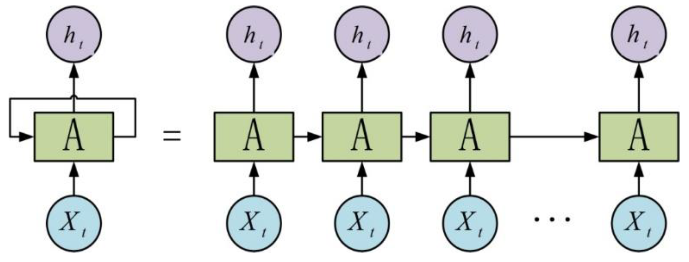
Recurrent Neural Network (RNN) is specialized for processing the series data. Compared with the classical feedforward neural network, the structure is relatively simple, which just reconnects the output of the hidden layer (or the output layer) back to the hidden layer forming a closed loop. It can also be considered as to add a memory unit in the feedforward neural network. When the neure transmits forward, the hidden layer does not only send messages to the front end, but also stores the message in the memory unit. When the next message performs, it will be sent to the hidden layer with the previous message stored in the memory units together to extract the features, and those processed messages will then be stored in the memory units again. The typical RNN model structure is as shown in Figure 1.
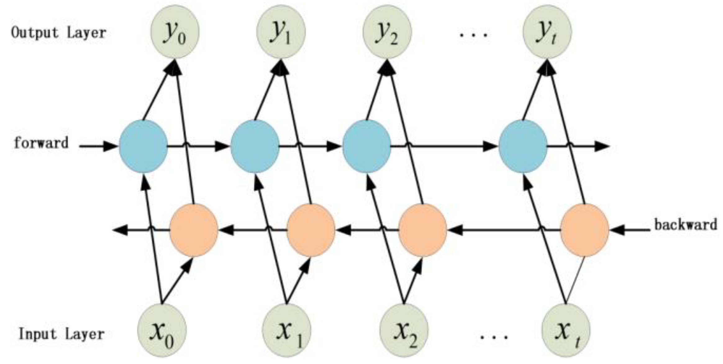
However, as the standard RNN is unidirectional, when processing the time series, the status value in the position is only related to output from position 0 to position , but has nothing to do with that from position i+1 to the end, namely information above only; to obtain the context information, RNN may calculate inversely to allow the status value in every position, and can obtain the information above from the forward RNN and the information below from the inverse RNN in order to make full use of the information in the past and the future. Such RNN is called bidirectional RNN, and according to which this paper proposed the Bi-directional Recurrent Neural Network (BRNN) [27]. The core conception of BRNN is that two RNNs will read the information from opposite directions with one starting from the beginning and the other starting from the end, as the series data are input into the model; the model will store the information respectively in two hidden layers connecting to the same output layer, and such a bidirectional recycle structure can provide every output series point in the output layer with the complete context information of the past and the future; namely the output of the neure in time depends on both the elements in the past and the future. Thereby, this model is able to visit the context information in the past as well as that in the future, and make full use of the input information during the model training. Whereas, RNN is incapable of providing the context information in the future. Theoretically, the input of BRNN contains three parts including the input from the input layer, as well as the previous-moment and next-moment output from the hidden layer. Consequently, the output layer can integrate perfectly the complete context information in every moment of the input series. The typical structure of BRNN is as shown in Figure 2.
From Figure 2, it is clear that the hidden layer of the network reserves two parts of information, namely the forward information , and the inverse information , while the final output contains both parts. is the output bias. Known from the three Equations above, the six unique weights including the weight matrix , (input layer to hidden layer), , (hidden layer to input layer) and , (hidden layer to hidden layer) are applied repeatedly in every moment, but each pair of the values between the forward and inverse is quite different.
2.2. The Vectorization of the Road Intersection
In the intelligent transportation system (ITS), the camera installation applied in recording the passing vehicles is involved. The cameras are installed in each road intersection with a unique serial number represented as ( is the integer between 0 and, and is the sum of the road intersections).
The data collected in every road intersection contain the information including the serial number of the road intersection, the vehicle numbers and time, which are the primary data for research. Since each vehicle passes through a different intersection in sequence, vehicle trajectory can be represented by a series of road intersection serial numbers sorted by time.
where is the number of the vehicle. is the road intersection serial number and is arranged according to the time sequence of the vehicles passing through the intersection. is the length of the vehicle track. In order to get the track data of each vehicle passing through the intersection serial number in a certain period of time, we need to process the original data into track data. Since the original data set is large, this paper adopts the trajectory data set statistical algorithm to generate the trajectory data (See Appendix A for the specific algorithm).
In the neural network training, as the intersection serial numbers of the traffic flow data are not in the vector form, they are unable to be directly input into the neural network, thus for the convenience of calculation and understanding of the neural network, the intersection serial number should be vectorized. This paper will regard each track data as a natural-language document with each intersection serial number as the single word in the document. Firstly, according to the data set the intersection serial numbers will be collected, which will be vectorized into the corresponding serial number after that. Finally, the vector matrix will be obtained depending on the vectorized intersection serial number. The vectorized serial number model can simplify the process of the text content into the vector operation in k-dimensional vector space, and the similarity in the vector space can be used to express the similarity of the text meaning [28]. This model connects all words to the hidden layer casting out the most time-consuming, nonlinear hidden layer, meanwhile inputting the word vector of the context of the testing word and outputting that of the testing word. As the large number of weight matrices need updating during the model training, which results in the excessive calculation, the training speed may possibly slow down. Therefore, to reduce the burden of training, this model integrates the negative sampling method which updates only the input and element weight in the negative sample set, and tends to considerably reduce the calculation amount during the gradient descent, and thereby accelerate the training speed [29].
Negative Sampling may generate a random negative example in the source code (the variate can be set in the code, and if the original word is generated during the random generation of the negative example, the number may possibly be less), where the original word is positive example with the label as 1, the other random generated label is 0, so the input is:
Loss is the negative Log likelihood (due to the random gradient descent method, here represents only a single layer in a word), namely:
The gradient can be expressed as follows:
The gradient transfer from the hidden layer to the output layer is even simpler, because the hidden layer is the sum of the variates in the input layer; thereby, the gradient of the input layer is namely that of the hidden layer.
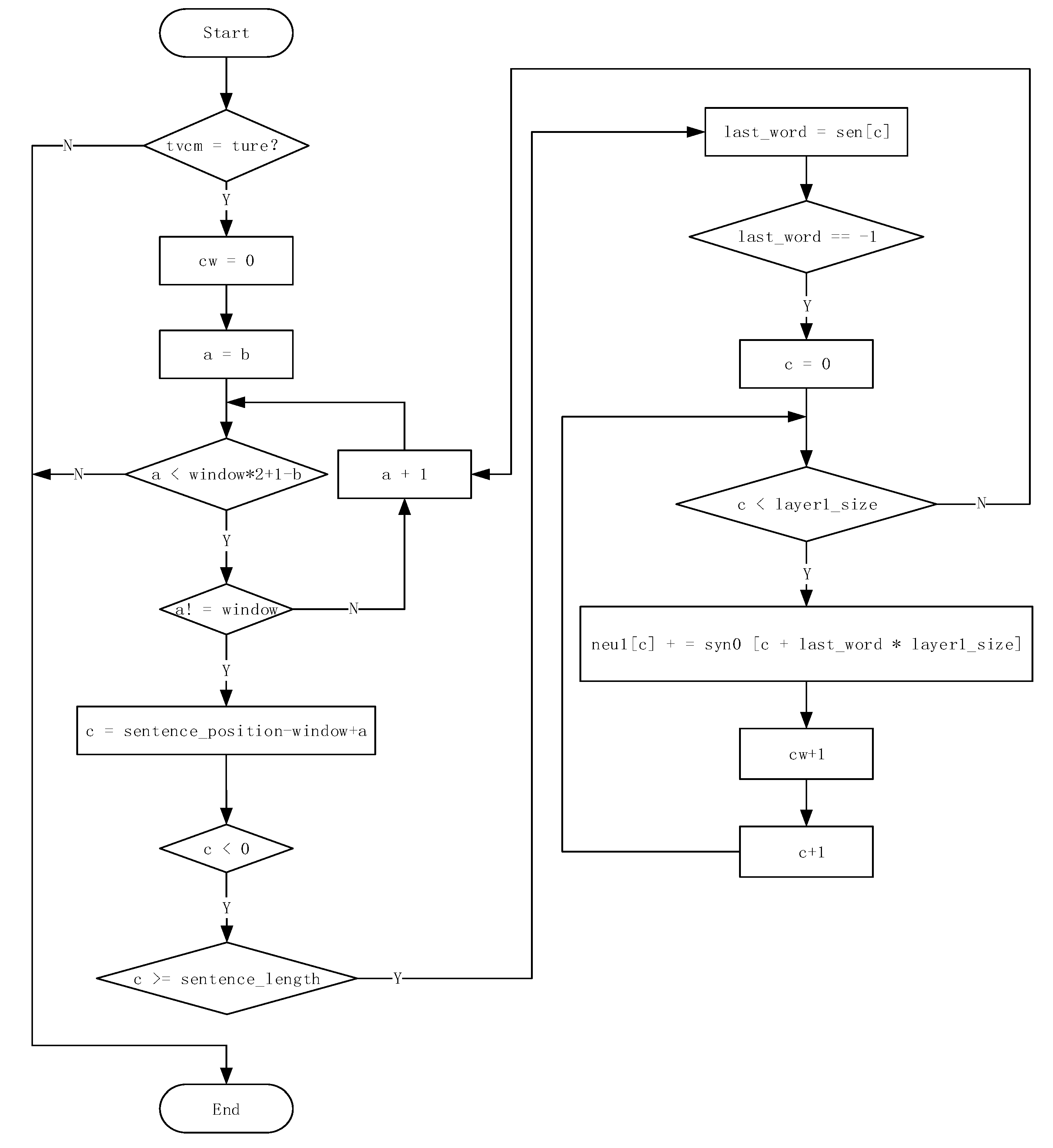
As shown in the Figure 3, the sentence position is the subscript of the current word in the sentence. Set the specific sentence A B C D as an example, when the code below is entered for the first time, the current word is A, its sentence position is 0. is the word generated randomly between 0 and window −1, and the size of entire window is (2 × window + 1 – 2 × b), which means to read window −b words on both the left and right side. It is obvious that with the window slipping from left to right the size is random, and when the random variation is from 3 (when b = window −1) to 2 (when b = 0), the random value b decides the size of the current window. In the code, nue1 is the vector of the hidden layer, namely the sum of the corresponding vector of the context (the words in the window except the current word.)
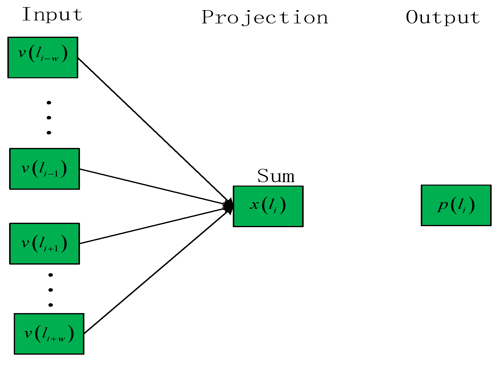
As shown in Figure 4, the prediction of the vectorized code model P (wt/wt−k, wt−(k−1), … wt−1, wt+1, wt+2, …, wt+k) can be obtained. The operation from input layer to the hidden layer is actually the sum of the context vector. The structure of the vectorized code model consists of four layers including the input layer, forward hidden layer, inverse hidden layer and the output layer, which is a discriminative model.
The core concept is the probability that the appearance of the current word will be maximum when the number of words appearing around the current word in the context is c, namely conditional probability maximization. When the words (the number of words is c) around the current two words tends to appear frequently, the vector of the two words will be very close, and the vector distance of this word will shrink.
Based on such a theory, it can be considered that in the date set constituted by the road intersection serial numbers, when the current vehicle is passing the testing road intersection, if the similar situation happens frequently in the adjacent road intersections, the relevance of those road intersections is high. Thereby, the spatial-tempo feature of the traffic flow can be fully manifested by the corresponding vector of the road intersection.
Where, is the vector of road intersection . is the step length. The Equation for the output of the projection layer and output layer is as follows:
The adjust equation of the vectorized code parameter based on the negative sampling is:
where, η is learning rate. NEG(li) is the negative sampling set. The update Equation of the vector of the input road intersection is:
This paper considers all track as the input of vectorized code model for the road intersection. The corresponding vector matrix for each track data is obtain by obtaining the corresponding vector of each road intersection serial number through training.
2.3. Calculation of Spatial Relations
The spatial relationship between intersections can be expressed by calculating the distance between the corresponding vectors of each intersection. The spatial closeness of any two intersections can be expressed by Equation (13).
For each intersection serial number, we calculated the Euclidean distance between and the corresponding vectors of other intersection serial numbers and sorted the results from smallest to largest. After this, we can get the serial number of intersections that are closest to it. Their serial number is. Combine them with , and the result is . The elements in this group are ordered from smallest to largest distance from the vector of the first intersection serial number (See Algorithm A2 in the Appendix A). Finally, the vehicle trajectory matrix of these intersections is input into the BRNN model for training and prediction. Such prediction results can not only reflect the close relationship between adjacent road intersections in traffic flow, but also reflect the spatial traffic flow relationship.
3. Experimental Results and Discussion
3.1. Data Description
This paper adopts the monitoring data of road intersections in partial sections in Shen Zhen, of which the list information of the intersection serial number includes six aspects—intersection serial number, ID of the monitoring point, name of the monitoring point, direction, the involved road and date. The passing vehicle record data in the intersections includes the plate number, vehicle color, time, the name of the monitoring point and the ID of the vehicle lane. Setting the intersection with the serial number 101000206 as the predicting point, nine intersection serial numbers with the closest relation to the predicting point are obtained by calculating the spatial relationship, as shown in Figure 5. Those ten intersections contain 3,469,741 primary data which were collected during 12 March 2018 to 1 April 2018. Through the trajectory data set statistic algorithm we obtained 725, 570 track data which were low-quality primary data with a different step length S for each track owing to the deviation during the data collection, such as equipment defect on certain intersections, identification error of the moving vehicle, failure of the information collection and position error of the moving vehicle, and so on. In order to solve those questions above, this paper input the corresponding vector matrix of the track data into the BRNN for training and prediction. BRNN will make full use of the historical and future information of the spatio-temporal series to predict the intersection serial number that the track actually passed. After several trainings, the model can obtain the high-quality track data, perform the counting statistics on the time of fixed step length, and thereby predict the traffic volume in the predicting intersection. Comparing the actual traffic volume on 1 April with the predicting value:
3.2. Error Evaluation Index
This paper uses mean square error (MSE) and accuracy (ACC) as evaluation indicators. The specific definition is as follows:
where: is the true value of traffic flow; is the predicted result; N is the number of predicted samples.
3.3. Result of the Intersection Vector
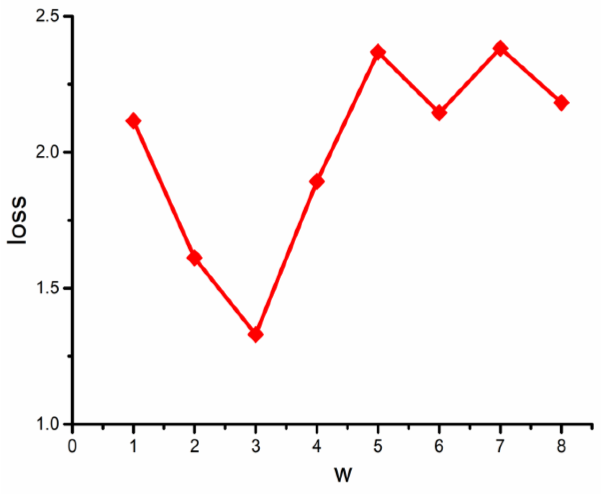
During the training of the vectorized mode model, the negative sampling set needed setting, which will be set as 10 here. In order to improve the training speed and the vector quality of the obtained word, the loss value of the vectorized code model with the different step length needs analyzing as well for a more accurate intersection vector. To analyze the variation rule of the loss value under a different step length, with the step length w between 1 and 8, after training experiments, the variation pattern of the loss value under different conditions can be summarized as shown in Figure 6.
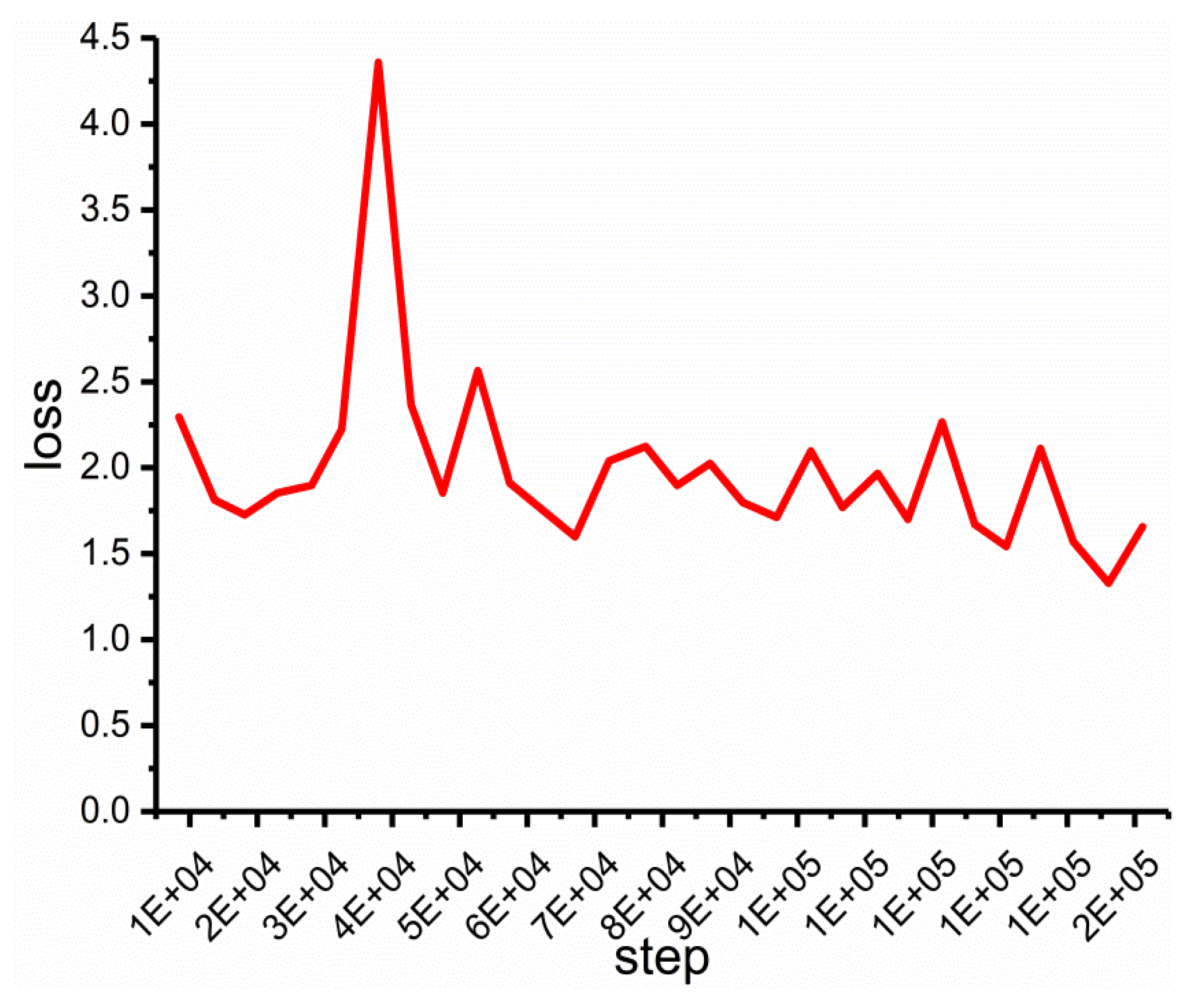
As known from the graph, the loss value meets a decrease before increasing, and slightly fluctuates after that. When is 3, this loss value reaches the bottom, and thereby the intersection vector is obtained by setting the step length as 3. Accordingly, the variation curve of the loss value with the iterations under the situation of negative sampling set being 10 and the step length being 3, is obtained as shown in Figure 7.
3.4. Result of BRNN Experiment
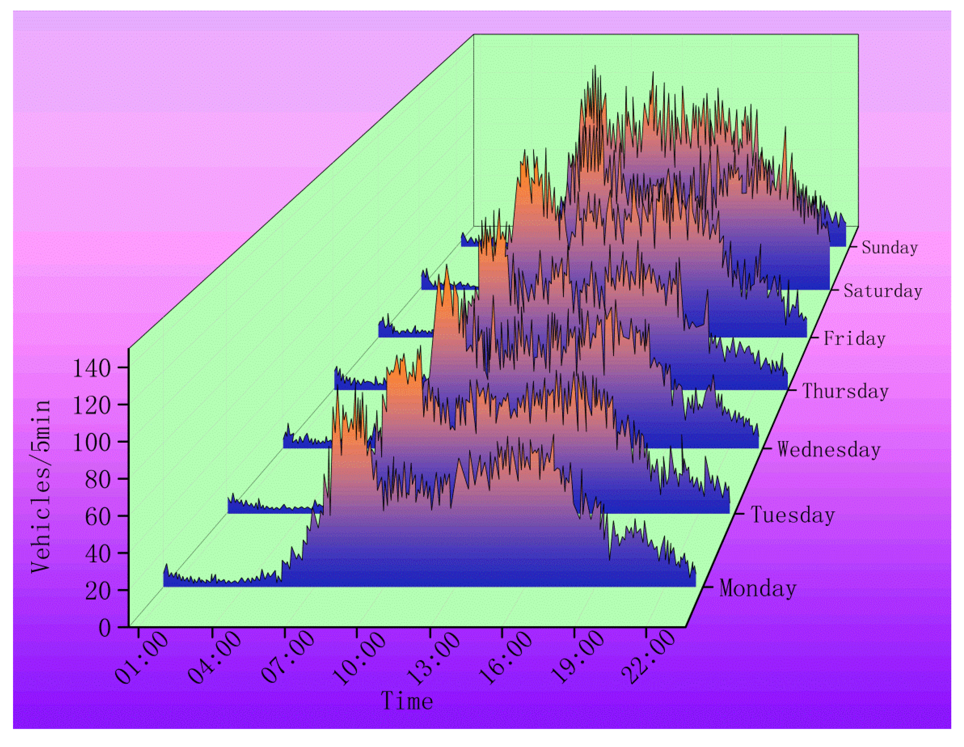
After a great deal of training of BRNN, the traffic volume on the predicting point (10100206) has been predicted during 25 March to 31 March, as shown in Figure 8.
As shown in Figure 8, the rush hour shows during 7 a.m. to 10 a.m. and 4 p.m. to 7 p.m. when the traffic is intense and the congestion is severe. According to the peak value and traffic intensity, traffic volume on Saturday and Sunday is considerably large. Accordingly, it is evident that the variation curve accords with the actually daily traffic situation.
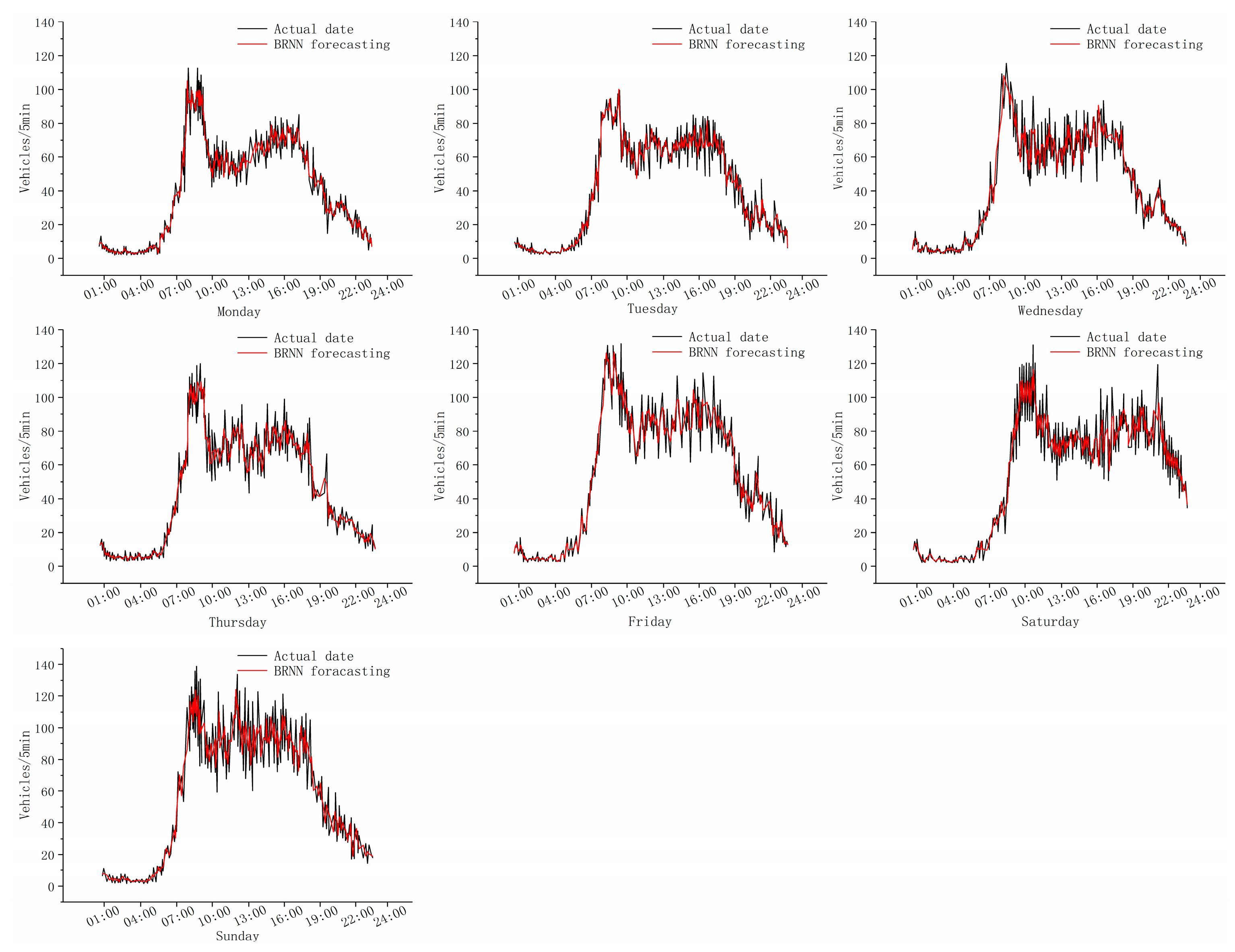
As shown in Figure 9, the predicting training results of the intersection (10100206) in one week reveal the deviation existing between the predicting results of BRNN and the true value. In order to more thoroughly analyze the predicting performance of BRNN, the RNN is trained as well during the training of the BRNN, and the result of comparison of the two models is as follows:
As shown in Figure 10, the result of BRNN is better than that of RNN. From the result of RNN, it is evident that RNN has higher similarity with short-term data series, but lower accuracy on long-term data series. This is because RNN cannot make use of the information in the past and the future of any specific moment, and thus will lose certain characteristics as the time runs longer, which tends to generate the predicting deviation.
3.5. Data Fitting and Residual Analysis
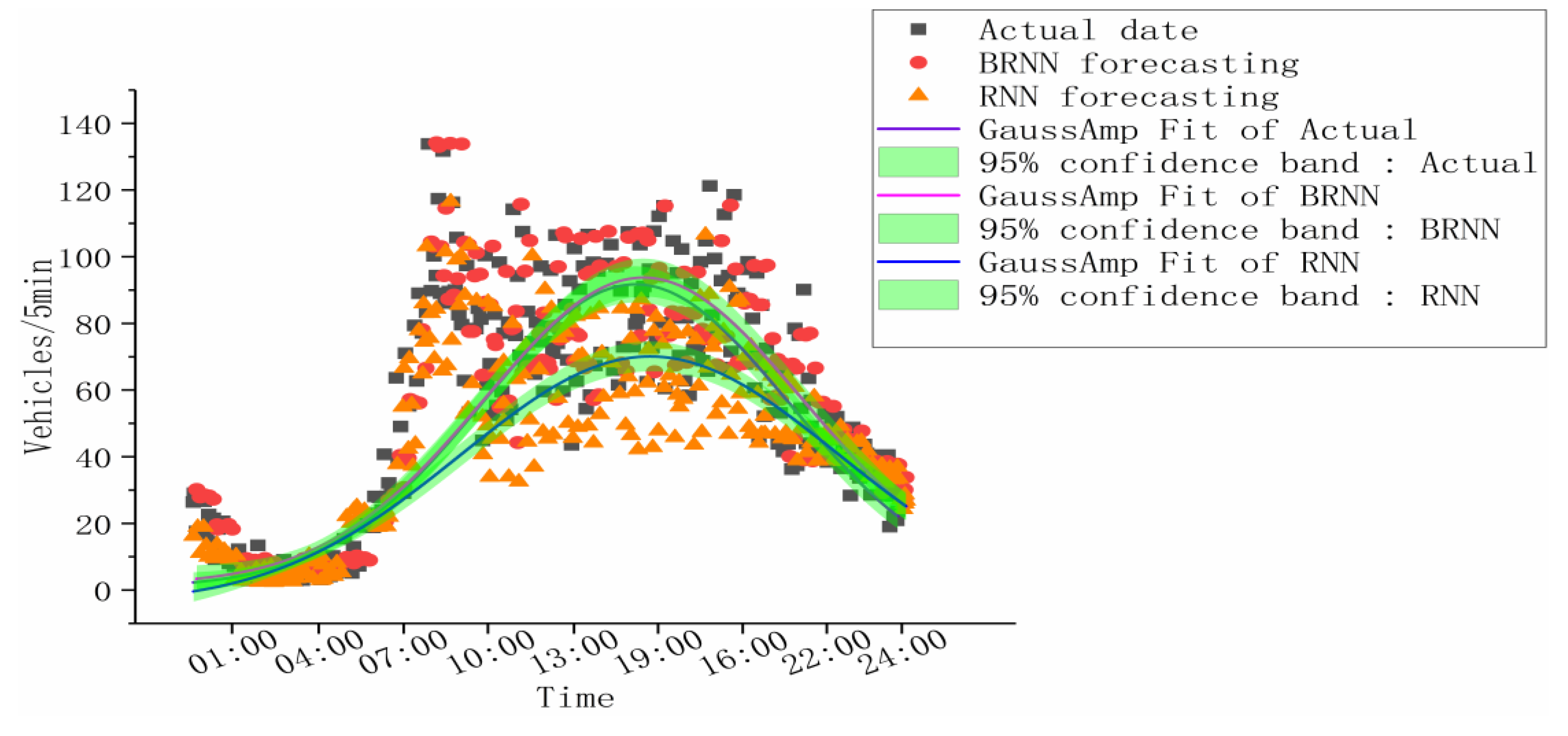
As shown in Figure 11, the discrete figure consists of three types of data on one coordination, and we fit those data by a nonlinear curve due to the nonlinear characteristic of the traffic flow, with GaussAmp as the fitting function during fitting to construct 95% of the confident belt, the Levenberg-Marquardt optimizing algorithm and the root of Reduced Chi-square to shrink the standard deviation. The result is as follows:
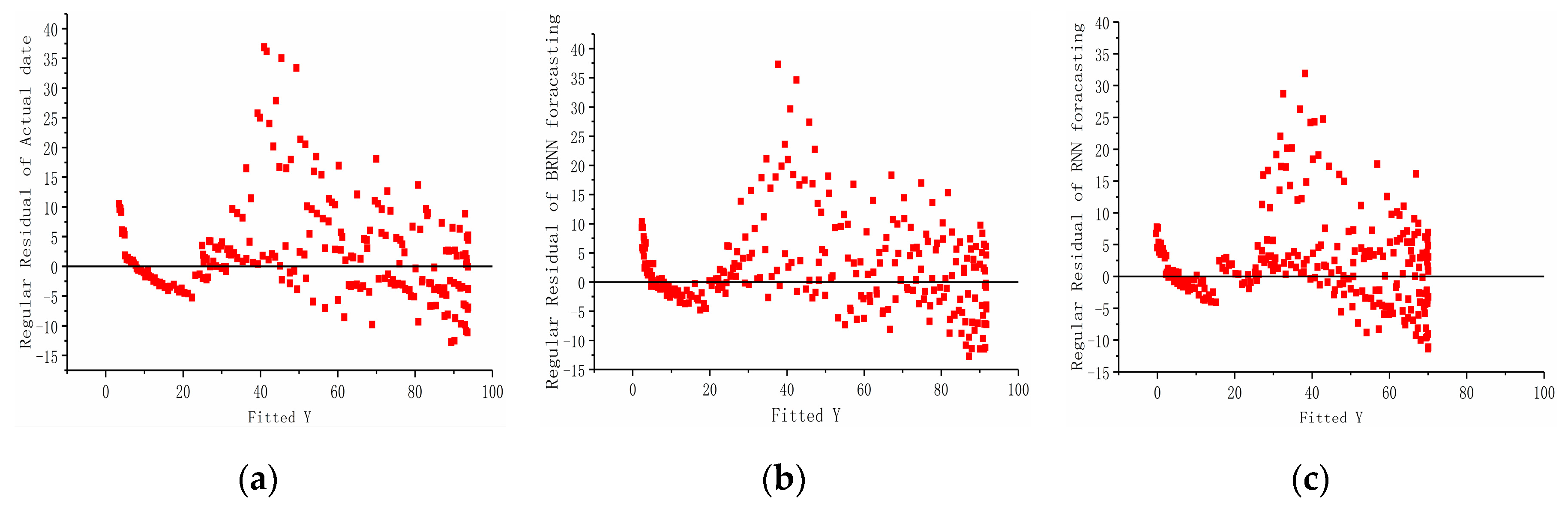
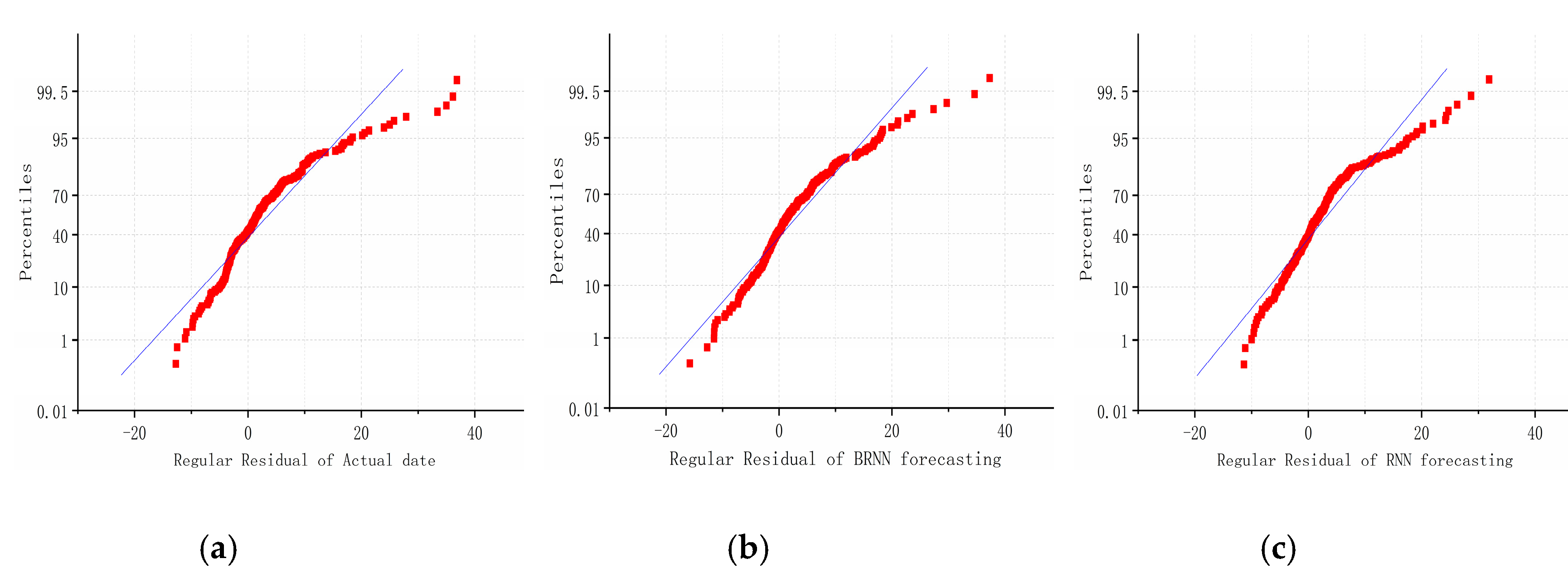
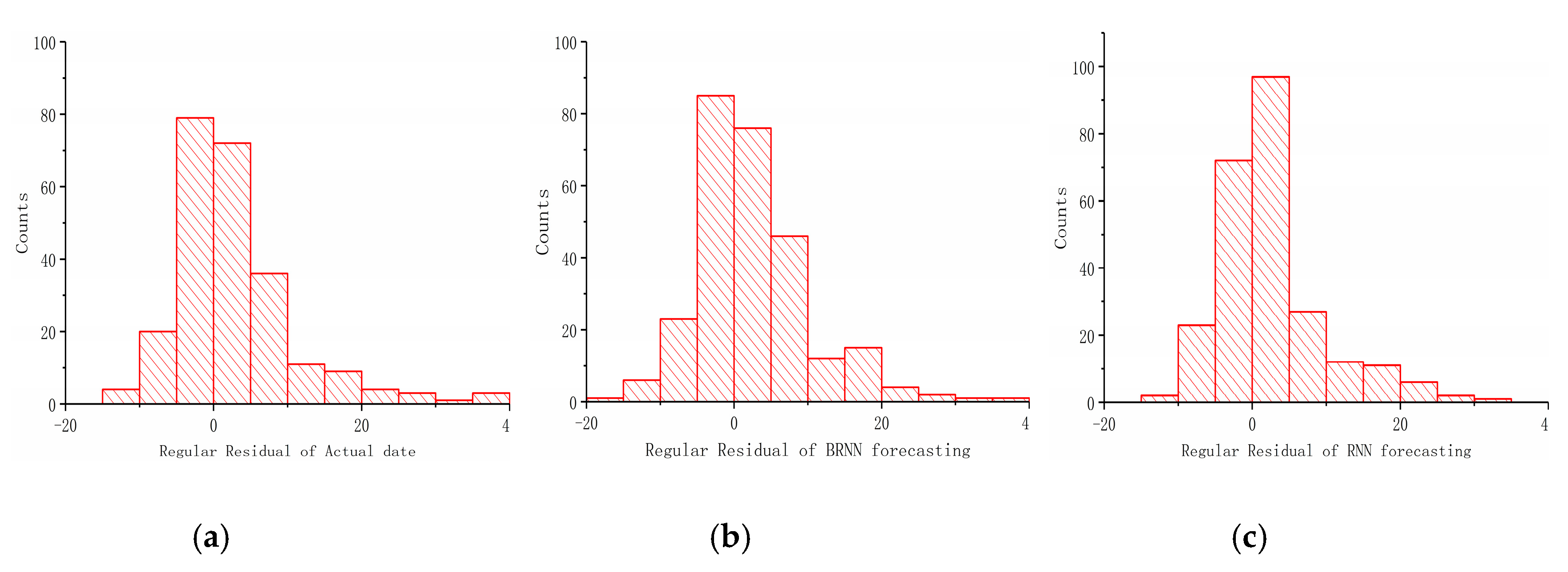
The fitting residual graphs of true value, BRNN and RNN, are shown as Figure 12, Figure 13 and Figure 14. The graphs show the result of fitting the Y value in the traffic flow prediction in the standard form, proportion form and column form. Comparing the intensity of the value near degree 0 in the three graphs, it is obvious that the density of BRNN is higher than RNN, thus with a better fitting result. In Figure 12, the fitting result of RNN is lower than expected due to the RNN being incapable to use the future information and losing part of data with input data becoming increasingly dense during training. However, the fitting result of BRNN is satisfied due to the capability of making full use of information in the past and the future, which makes the predicting result close to the true value. In Figure 13, all data points are distributed around the diagonal line, and the data point from BRNN is closer to the line with high density, and thus less deviation. In Figure 14 the column graphs of three predicting results reveal that the prediction of BRNN is closer to the true traffic volume.
The Equations used in the data fitting are shown in Table 1. The fitting results of the data are shown in Table 2.
From the squared value of the correlation coefficient R (COD) of the BRNN and RNN, it is apparent that the closer the squared value of R is to 0, the better the fitting degree. When the squared value of R of the BRNN and RNN are 7.40129 and 6.03239, respectively, that of BRNN is much closer to 1, and thus the deviation between the curve after fitting and the primary data point is smaller, and the prediction is more accurate. As to the residual sum of squares, that of BRNN is obviously larger than that of RNN, which means BRNN is better.
3.6. The Effect of Track Length on the Model
In data collection, due to the error of the acquisition equipment (or other error factors), we get the wrong original data. The original data can be processed to obtain the track data, and the vector matrix corresponding to the track data can be used as the input of the model for training and prediction. Therefore, when errors occur in the collected data, the most significant impact on the model is the accuracy of prediction results. Let us discuss how error data affects model accuracy. In other words, explore the influence of trajectory lengthcon model accuracy.
As shown in Section 2.2, this is the number of intersections, so when the data is wrong, we get that the length of the trajectory will change or stay the same. In this case, it reduces the track collection density, affects the description of moving vehicle tracks, and also gets the wrong track data. Therefore, it is equivalent to discussing the influence of on model accuracy.
There are two cases of the most common trajectory missing (we only discuss the most common cases). For example, if the HD camera fails, it will not work properly. At this time, the serial number of the road intersection of the trajectory data will be missing, and the track length will become smaller. In another case, when the camera recognizes an error in the license plate number, the serial number of the intersection does not change, but the identified vehicle is no longer a real vehicle.
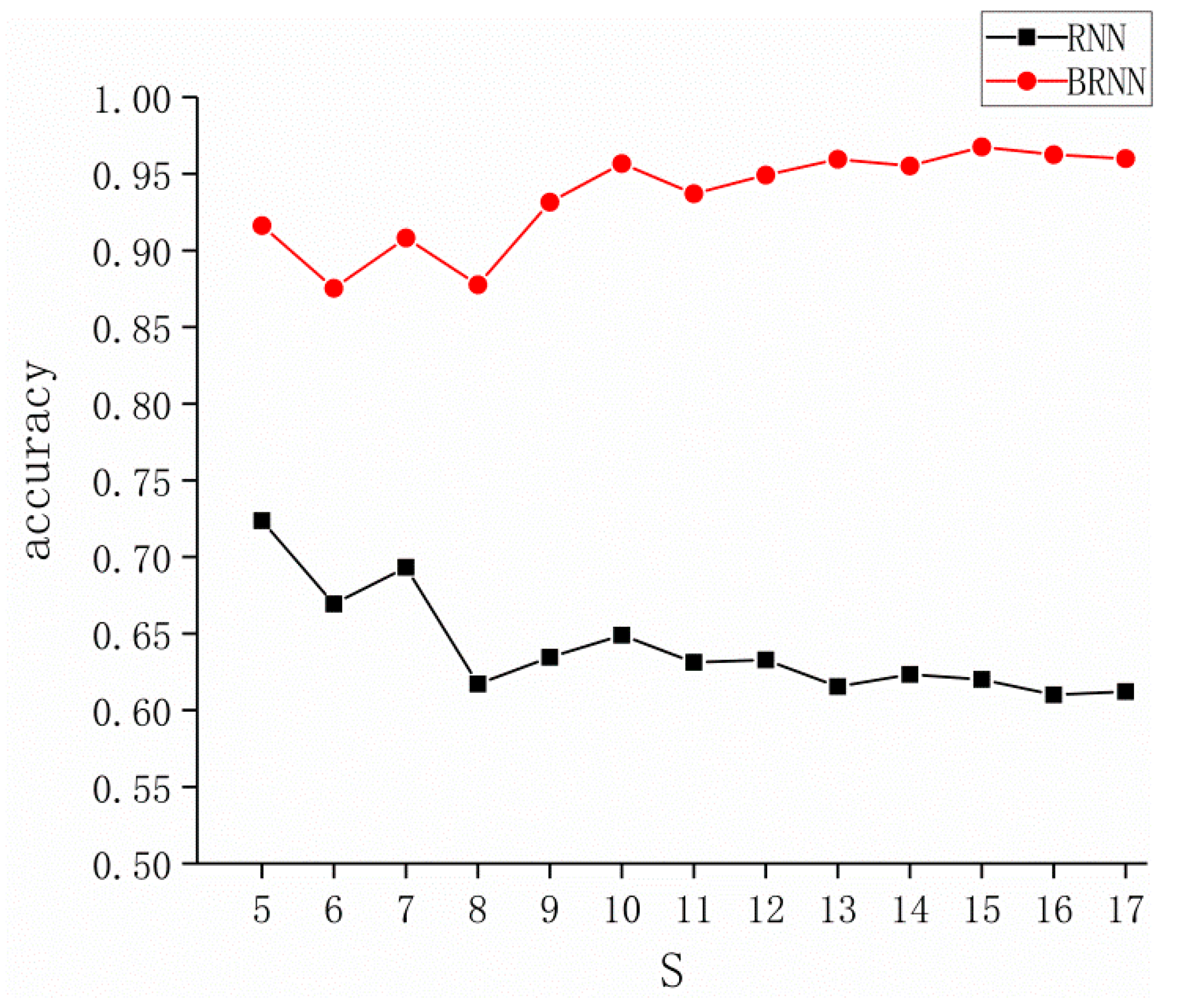
When changes. We select the trajectory of. Because when the trajectory length is less than 5, the trajectory does not reflect the moving characteristics of the vehicle between road intersections (If there are too many such trajectories, it can be inferred that the damage of the collection equipment is too serious. It is recommended that the equipment at the intersection be inspected and repaired). Set the default length of the track length to 7 (value range is 5, 7, 8, 9, 10, 11, 12, 13, 14, 15, 16, 17) to compare the accuracy of the model at different track lengths. The result is shown in the Figure 15.
As shown in the above figure, the accuracy of the BRNN model is relatively low at the beginning and fluctuates strongly, and then becomes a slow upward trend, then slowly stabilizes, while RNN is reversed. When , the BRNN model has the lowest accuracy rate of 87.53%. When , the BRNN model has the highest accuracy rate of 96.75%.
In summary, when there are more errors in data collection, will become smaller. As a result, the accuracy of the BRNN model is reduced, and the magnitude of the change is large, which is an unstable state.
When S does not change. Due to camera recognition error. For example, the real license plate number AT6351 is incorrectly identified as AT63S1. The track length S thus acquired is constant, and the prediction accuracy obtained after the model training is higher than the true accuracy. Therefore, the BRNN model has to do more work. This work is to repair the trajectory. This will result in an increase in the computation time of the model (After the track data is repaired, it has little influence on the prediction accuracy of the model and can be ignored).
In order to further assess the predicting performance of BRNN, this paper calculates the predicting results of MSE and ACC, respectively, and makes comparison with RNN, ARIMA, SVR, DBN-SVR, LSTM and KNN-LSTM [30]. The results are shown as in Table 3 that BRNN processes the best predicting performance with an accuracy of 96.75%, which is 24.34%, 25.06, 8.58%, 7.15% and 6.36% higher than RNN, ARIMA, SVR, DNB-SVR and LSTM, respectively. Meanwhile compared with KNN-LSTM, which takes into account the spatio-temporal relationship, the accuracy improves 2.16% as well. Consequently, this experiment illustrates that BRNN has excellent predicting performance.
4. Conclusions
Based on the deep learning theory, this paper proposed the Bi-directional Regression Neural Network, which can make full use of the intersection information in the past and the future to make up the deficiency of most other models that they are incapable to reflect the spatio-temporal relation of the traffic flow. Meanwhile, this paper, according to the TensorFlow platform, designed the vectorized code to extract the spatial feature of the intersections and to screen out the intersections related closely to the predicting point, as well as to train and predict through inputting the track vector matrix of those intersections into the BRNN. This paper also carried out the predicting data fitting of BRNN and RNN, and the residual analysis. The results indicated that the BRNN can make full use of the information in the past and future to process better performance, whose accuracy is up to 96.75%. In addition, this paper made the compassion of the deviation between BRNN and RNN, ARIMA, SVR, DBN-SVR and LSTM, as well as KNN-LSTM, and the consequences show that the accuracy of BRNN is 16.298% higher on average, which further proved the excellent predicting performance of BRNN.
Author Contributions
Conceptualization, S.Z. and Q.Z.; Data curation, S.Z. and Q.Z.; Formal analysis, S.Z. and Q.Z.; Funding acquisition, S.Z. and S.L.; Investigation, Q.Z. and Y.B.; Methodology, S.Z. and Q.Z.; Project administration, S.Z.; Resources, Q.Z. and Y.B.; Software, S.Z., Q.Z. and S.L.; Supervision, S.Z.; Validation, S.Z., Q.Z. and S.L.; Writing – original draft, Q.Z.; Writing – review & editing, Y.B.
Funding
This research was supported by the Shaanxi Provincial Education Department serves Local Scientific Research Plan in 2019 (Project NO.19JC028) and Shaanxi Provincial Key Research and Development Program (Project NO.2018ZDCXL-G-13-9) and Shaanxi province special project of technological innovation guidance (fund) (Program No.2019QYPY-055).
Conflicts of Interest
The authors declare no conflict of interest.
Appendix A
| Algorithm A1. Trajectory data set statistical algorithm. |
| map: |
| map (key, value, context): |
| passRecord = value. split(); |
| for pr in passRecord: |
| context. write(pr. vehicleNo, pr. locationId); |
| reduce: |
| reduce (key, values, context): |
| result = temp; |
| for value in values; |
| result.append (value); |
| context.write(key, result); |
| //The final output is < vehicle ID, intersection serial number list > |
| Algorithm A2. The algorithm of spatial closeness. |
| G = Empty collection; |
| for la in L: //L is the set of all intersection serial number |
| list<lx, distance(la, lx)>1; |
| for lx in L: |
| if(lx ≠ la): |
| d = distance(la, lx); |
| 1.put(lx, d); |
| 1.sortByValues();//Sort by distance |
| Ga = 1.top(k) ∪ la;//Banked the nearest k intersection serial number collection |
| G = G ∪ Ga; |
| return G; |
References
- Zambrano-Martinez, J.L.; Calafate, C.T.; Soler, D.; Lemus-Zúñiga, L.-G.; Cano, J.-C.; Manzoni, P.; Gayraud, T. A Centralized Route-Management Solution for Autonomous Vehicles in Urban Areas. Electronics 2019, 8, 722. [Google Scholar] [CrossRef]
- Shaikh, R.A.; Thayananthan, V. Risk-Based Decision Methods for Vehicular Networks. Electronics 2019, 8, 627. [Google Scholar] [CrossRef]
- Botte, M.; Pariota, L.; D’Acierno, L.; Bifulco, G.N. An Overview of Cooperative Driving in the European Union: Policies and Practices. Electronics 2019, 8, 616. [Google Scholar] [CrossRef]
- Kalamaras, I.; Zamichos, A.; Salamanis, A.; Drosou, A.; Kehagias, D.D.; Papadopoulos, S.; Tzovaras, D. An interactive visual analytics platform for smart intelligent transportation systems management. IEEE Trans. Intell. Transp. Syst. 2017, 19, 1–10. [Google Scholar] [CrossRef]
- Shuanfeng, Z.; Wei, G.; Chuanwei, Z. Extraction Method of Driver’s Mental Component Based on Empirical Mode Decomposition and Approximate Entropy Statistic Characteristic in Vehicle Running State. J. Adv. Transp. 2017, 2017, 1–14. [Google Scholar]
- Zhao, S. The implementation of driver model based on the attention transfer process. Math. Probl. Eng. 2017, 2017, 15. [Google Scholar] [CrossRef]
- Gang, Y.; Le, W.; Lizhen, D.; Fangping, X. Traffic Flow Prediction Based on Adaptive Particle Swarm Optimization of Least Square Support Vector Machine. Control Eng. China 2017, 24, 1838–1843. [Google Scholar]
- Sheng, N.; Tang, U.W. Spatial Analysis of Urban Form and Pedestrian Exposure to Traffic Noise. Int. J. Environ. Res. Public Health 2011, 8, 1977–1990. [Google Scholar] [CrossRef] [PubMed]
- Kumar, S.V.; Vanajakshi, L. Short-term traffic flow prediction using seasonal ARIMA model with limited input data. Eur. Transp. Res. Rev. 2015, 7, 21. [Google Scholar] [CrossRef]
- Dihua, S.; Chao, L.; Xiaoyong, L. An Improved Nonparametric Regression Algorithm for Short-term Expressway Traffic Flow Forecasting. J. Highw. Transp. Res. Dev. 2013, 30, 112–118. [Google Scholar]
- Yu, W.; Su, J.; Zhang, W. Research on Short-Time Traffic Flow Prediction Based on Wavelet de-Noising Preprocessing. In Proceedings of the IEEE Ninth international Conference on Natural Computation, Shenyang, China, 23–25 July 2013; pp. 252–256. [Google Scholar]
- Li, L.; He, S.; Zhang, J.; Ran, B. Short-term highway traffic flow prediction based on a hybrid strategy considering temporal-spatial information. J. Adv. Transp. 2016, 50, 2029–2040. [Google Scholar] [CrossRef]
- Mikolov, T.; Sutskever, I.; Chen, K.; Corrado, G.S.; Dean, J. Distributed Representations of Word and their Compositionality. In Proceedings of the Advances in Neural Information Processing Systems, Stateline, NV, USA, 5–10 December 2013; pp. 3111–3119. [Google Scholar]
- Lee, C.-H.; Chih-Hung, W. A Novel Big Data Modeling Method for Improving Driving Range Estimation of EVs. IEEE Access 2015, 3, 1980–1993. [Google Scholar] [CrossRef]
- Xiaobo, C.; Xiang, L.; Zhongjie, W.; Jun, L.; Yingfeng, C.; Long, C. Short-term Traffic Flow Forecasting of Road Network Based on GA-LSSVR Model. J. Transp. Syst. Eng. Inf. Technol. 2017, 17, 60–66. [Google Scholar]
- Ma, X.; Yu, H.; Wang, Y.; Wang, Y. Large-scale transportation network congestion evolution prediction using deep learning theory. PLoS ONE 2015, 10, e0119044. [Google Scholar] [CrossRef] [PubMed]
- Xuankun, D.; Liang, W.; Hongwei, D.; Zhuang, X. Traffic Flow Prediction Based on Deep Neural Networks. Comput. Eng. Appl. 2019, 55, 228–235. [Google Scholar]
- Mackenzie, J.; Roddick, J.F.; Zito, R. An Evaluation of HTM and LSTM for Short-Term Arterial Traffic Flow Prediction. IEEE Trans. Intell. Transp. Syst. 2019, 20, 1847–1857. [Google Scholar] [CrossRef]
- Feldman, O. The GEH Measure and Quality of the Highway Assignment Models; Association European Transport: Glasgow, Scotland, UK, 2012. [Google Scholar]
- Tian, Y.; Pan, L. Predicting short-term traffic flow by long short-term memory recurrent neural network. In Proceedings of the IEEE international conference on smart city/SocialCom/SustainCom (SmartCity), Chengdu, China, 19–21 December 2015; pp. 153–158. [Google Scholar]
- Pamuła, T. Classification and prediction of traffic flow based on real data using neural networks. Arch. Transp. 2012, 24, 519–529. [Google Scholar] [CrossRef]
- Pamuła, T. Short-term traffic flow forecasting method based on the data from video detectors using a neural network. In Activities of Transport Telematics (Communications in Computer and Information Science); Springer: Berlin, Germany, 2013; pp. 147–154. [Google Scholar]
- Huang, W.; Song, G.; Hong, H.; Xie, K. Deep architecture for traffic flow prediction: Deep belief networks with multitask learning. IEEE Trans. Intell. Transp. Syst. 2014, 15, 2191–2201. [Google Scholar] [CrossRef]
- Halawa, K.; Bazan, M.; Ciskowski, P.; Janiczek, T.; Kozaczewski, P.; Rusiecki, P. Road traffic predictions across major city intersections using multilaye perceptrons and data from multiple intersections located in various places. IEEE Trans. Intell. Transp. Syst. 2016, 10, 469–475. [Google Scholar] [CrossRef]
- Guo, J.; Huang, W.; Williams, B.M. Adaptive Kalman filter approach for stochastic short-term traffic flow rate prediction and uncertainty quantification. Transp. Res. C Emerg. Technol. 2014, 43, 50–64. [Google Scholar] [CrossRef]
- Min, W.; Wynter, L. Real-time road traffic prediction with spatiotemporal correlations. Transp. Res. C Emerg. Technol. 2011, 19, 606–616. [Google Scholar] [CrossRef]
- Schuster, M.; Paliwal, K.K. Bidirectional Recurrent Neural Networks. IEEE Trans. Signal Process. 1997, 11, 2673–2681. [Google Scholar] [CrossRef]
- Mikolov, T.; Chen, K.; Corrado, G.; Dean, J. Efficient Estimation of Word Representations in Vector Space. arXiv 2013, arXiv:1301.3781. [Google Scholar]
- Mikolov, T.; Sutskever, I.; Chen, K.; Corrado, G.; Dean, J. Distributed Representations of Word and Phrases and their Compositionality. In Proceedings of the 26th International Conference on Neural Information Processing Systems, Lake Tahoe, NV, USA, 5–10 December 2013. [Google Scholar]
- Luo, X.; Li, D.; Yu, Y.; Zhang, S. Short-term traffic flow prediction based on KNN-LSTM. J. Beijing Univ. Technol. 2018, 44, 1521–1527. [Google Scholar]
Figure 1.
Computation flow of RNN model.

Figure 2.
Computation flow of Bi-directional Regression Neural Network (BRNN) model.

Figure 3.
Part of the source code flow chart of the vectorization coding model.

Figure 4.
Calculation process the vectorization coding model.

Figure 5.
Distribution and ID of intersections in the testing road network.

Figure 6.
Linear graph of loss variation.

Figure 7.
Curve of loss value varying with iterations.

Figure 8.
The predicted value in a week.

Figure 9.
The comparison results of predicted and real traffic flow in a week’s time.

Figure 10.
This is the model prediction curves of RNN and BRNN. This first graph (a) is the comparison diagram of real traffic flow and predicted traffic flow by RNN, while the second (b) is the comparison diagram of real traffic flow and predicted traffic flow by BRNN.
Figure 10.
This is the model prediction curves of RNN and BRNN. This first graph (a) is the comparison diagram of real traffic flow and predicted traffic flow by RNN, while the second (b) is the comparison diagram of real traffic flow and predicted traffic flow by BRNN.

Figure 11.
Fitting curve of the scatter value.

Figure 12.
This is the residual diagram of the predicted results for each model. The graph (a) is the regular residual of actual data under the fitted Y value. That of (b) is the regular residual of BRNN model under the fitted Y value. The one of (c) is the regular residual of RNN model under the fitted Y value.

Figure 13.
The graph designated (a) is the regular residual of actual data under the percentiles form, (b) is the regular residual of BRNN forecasting under the percentiles form, and (c) is the regular residual of RNN forecasting under the percentiles form.
Figure 13.
The graph designated (a) is the regular residual of actual data under the percentiles form, (b) is the regular residual of BRNN forecasting under the percentiles form, and (c) is the regular residual of RNN forecasting under the percentiles form.

Figure 14.
This is a histogram of regular residual of traffic flow prediction results. Graph (a) is a histogram regular residual of the actual data. Graph (b) is a histogram regular residual of the BRNN model. Graph (c) is a histogram regular residual of the RNN model.
Figure 14.
This is a histogram of regular residual of traffic flow prediction results. Graph (a) is a histogram regular residual of the actual data. Graph (b) is a histogram regular residual of the BRNN model. Graph (c) is a histogram regular residual of the RNN model.

Figure 15.
Accuracy of the model for different values.


Table 1.
Models and equations used in the fitting.
| Model | Equation |
|---|---|
| GaussAmp |
Table 2.
Data table of fitting results.
| Plot | Actual Date | BRNN Forecasting | RNN Forecasting |
|---|---|---|---|
| 0.8452 ± 2.02181 | 1.70427 ± 2.6873 | −4.33261 ± 2.886 | |
| 9.08585 ± 0.0815 | 9.229 ± 0.08364 | 0.34728 ± 0.1072 | |
| 2.7974 ± 0.12182 | 2.87558 ± 0.1420 | 3.42083 ± 0.2021 | |
| 90.87526 ± 2.808 | 92.04544 ± 3.179 | 74.42464 ± 2.888 | |
| Reduced Chi-Square | 8.64135 | 7.40129 | 6.03239 |
| R-square(COD) | 0.80646 | 0.79486 | 0.79342 |
| ADJ.R-square | 0.8043 | 0.79227 | 0.79093 |
| Residual sum of squares | 96066.57313 | 90180.34987 | 68932.96234 |
Table 3.
Prediction performance of different models.
| Prediction Model | The Evaluation Index | |
|---|---|---|
| MSE | ACC/% | |
| ARIMA | 1.5134 | 61.09 |
| RNN | 0.7365 | 72.36 |
| SVR | 0.3266 | 88.17 |
| DBN-SVR | 0.3053 | 89.60 |
| LSTM | 0.1262 | 90.39 |
| KNN-LSTM | 0.0987 | 94.59 |
| BRNN | 0.0831 | 96.75 |
© 2019 by the authors. Licensee MDPI, Basel, Switzerland. This article is an open access article distributed under the terms and conditions of the Creative Commons Attribution (CC BY) license (http://creativecommons.org/licenses/by/4.0/).
Share and Cite
MDPI and ACS Style
Zhao, S.; Zhao, Q.; Bai, Y.; Li, S. A Traffic Flow Prediction Method Based on Road Crossing Vector Coding and a Bidirectional Recursive Neural Network. Electronics 2019, 8, 1006. https://doi.org/10.3390/electronics8091006
AMA Style
Zhao S, Zhao Q, Bai Y, Li S. A Traffic Flow Prediction Method Based on Road Crossing Vector Coding and a Bidirectional Recursive Neural Network. Electronics. 2019; 8(9):1006. https://doi.org/10.3390/electronics8091006
Chicago/Turabian StyleZhao, Shuanfeng, Qingqing Zhao, Yunrui Bai, and Shijun Li. 2019. "A Traffic Flow Prediction Method Based on Road Crossing Vector Coding and a Bidirectional Recursive Neural Network" Electronics 8, no. 9: 1006. https://doi.org/10.3390/electronics8091006
Note that from the first issue of 2016, this journal uses article numbers instead of page numbers. See further details here.