Performance Analysis of Low-Level and High-Level Intuitive Features for Melanoma Detection
by
 ,
,
Muniba Ashfaq
1, 
Nasru Minallah
1,*,
Zahid Ullah
2,*,
Arbab Masood Ahmad
1,
Aamir Saeed
3 and
Abdul Hafeez
1,3,* 1
Department of Computer Systems Engineering, University of Engineering & Technology, Peshawar 54890, Pakistan
2
Department of Electrical Engineering, CECOS University of IT & Emerging Sciences, Peshawar 25000, Pakistan
3
Departmnt of Computer Science & IT, University of Engineering & Technology, Jalozai Campus, Khyber Pakhtunkhwa 24240, Pakistan
*
Authors to whom correspondence should be addressed.
Electronics 2019, 8(6), 672; https://doi.org/10.3390/electronics8060672
Submission received: 27 May 2019
/
Revised: 7 June 2019
/
Accepted: 7 June 2019
/
Published: 13 June 2019
(This article belongs to the Section Bioelectronics)
Abstract
:This paper presents an intelligent approach for the detection of Melanoma—a deadly skin cancer. The first step in this direction includes the extraction of the textural features of the skin lesion along with the color features. The extracted features are used to train the Multilayer Feed-Forward Artificial Neural Networks. We evaluate the trained networks for the classification of test samples. This work entails three sets of experiments including , and of the data used for training, while the remaining , and constitute the test sets. Haralick’s statistical parameters are computed for the extraction of textural features from the lesion. Such parameters are based on the Gray Level Co-occurrence Matrices (GLCM) with an offset of and 28, each with an angle of and 135 degrees, respectively. In order to distill color features, we have calculated the mean, median and standard deviation of the three color planes of the region of interest. These features are fed to an Artificial Neural Network (ANN) for the detection of skin cancer. The combination of Haralick’s parameters and color features have proven better than considering the features alone. Experimentation based on another set of features such as Asymmetry, Border irregularity, Color and Diameter (ABCD) features usually observed by dermatologists has also been demonstrated. The ‘D’ feature is however modified and named Oblongness. This feature captures the ratio between the length and the width. Furthermore, the use of modified standard deviation coupled with ABCD features improves the detection of Melanoma by an accuracy of
1. Introduction
Skin cancer is the most common form of cancer types. It is generally divided into two categories: melanoma (5%) and nonmelanoma (95%). However, melanoma is the most serious skin cancer because of its strong ability to metastasize. This skin cancer is primarily linked to overexposure to ultraviolet light. Therefore, early detection offers better chances of cure, hence the value of this melanoma detection study.
1.1. Motivation
Skin cancer is the most spread cancer in US [1,2]. According to American Cancer Society (Cancer Facts and Figures 2018), estimation of 91,270 new cases will be diagnosed and 9320 deaths will occur in 2018. A five-year survival rate for early detection and treatment of melanoma is . Excision of malignant (cancerous) tissue can heal a melanoma patient at an early stage of the disease. Benign (non-cancerous) tumors often develop in melanocytes. These benign tumors appear in the form of moles (nevi) and has much resemblance with melanoma. Doctors face difficulty in differentiating benign tumors from melanoma. They use the ABCD rule; and their experience for the detection of melanoma. Friedman et al. was the first one to use “ABCD” features for early detection of melanoma [3]. The mnemonic stands for Asymmetry, Border irregularity, Color and Diameter. A Melanoma lesion is asymmetric, has an irregular border, has color variation containing different shades and combinations of black, brown and tan and its diameter is greater than 6 mm.
1.2. Contributions
In our research, we have done a comprehensive analysis on performance of skin cancer detection with ANN using Low-Level Intuitive Features (LLIF) and High-Level Intuitive Features (HLIF), which is summarized as follows:
- GLCM parameters that include contrast, energy, homogeneity and correlation are extracted from both dermIS and dermQuest dataset. Analysis is done using data split of 50%:50%, 70%:30% and 90%:10% for training:test data. Experiment is repeated ten times to evaluate the accuracy using 10 random seeds.
- Analysis of varying GLCM offsets (2, 4, 8, 12, 16, 20, 24, 28) to measure the performance of ANN for skin cancer detection.
- Color features are extracted from each color plane (red, green and blue) and are considered as statistical features. These include mean, median and standard deviation. Color features are applied to ANN as input with the best random seed selected through varying seed analysis.
- Consequently, GLCM and color features are used as consolidated features to evaluate the performance with varying data split for training:test data.
- ABCD (Asymmetry, Border Irregularity, Color, Diameter) features are used as input to ANN for performance analysis. The color factor is computed using statistical features (mean, median, standard deviation) from each color plane.
- Diameter features from ABCD is taken as Oblongness factor which is mostly ignored in literature. The diameter changes with changes in the distance of lesion and image acquisition system.
- Comparison of LLIF and HLIF using ANN for skin cancer detection has been shown.
- The optimal parameter settings of GLCM offset, ANN training and test data split and the effect of varying random seed have been concluded from the analysis.
- A modified standard deviation, a novel way of computing standard deviation from an image, described in Section 4.1, results in a single value of standard deviation, which proves to be better than conventional standard deviation. The accuracy found using the modified standard deviation is .
The research paper is organized as follows. Past work done in the field of skin cancer detection is presented in Section 2. All phases of skin cancer detection are included in Section 3. Section 4 describes the implementation details of this research work. Section 5 describes the evaluation and experimental results. Section 6 summarizes the work done in this paper and the pros and cons of using the different features of skin cancer. Section 7 concludes the paper giving directions for the future research.
2. Literature Survey
Skin cancer can be detected by using High Level Intuitive Features (HLIF) and Low Level Intuitive Features (LLIF). HLIF are the features that mathematically model human observation for specific characteristics or attributes of a lesion and are generally used for classification e.g., ABCD rule produces the HLIF and is used by physicians. LLIF are not intended to formulate natural human observation to a specific attribute for classification problem. Robert Amelard et al. [6] used HLIF for the classification of skin lesion using standard camera images. Nishu Rani et al. [7] extracted features from skin lesion using 2D wavelet transform [8]. The features consisting of mean, standard deviation, mean absolute deviation, L1 norm and L2 norm were applied to a back propagation neural network for classification. Abdul Jaleel et al. [9] produced Gray Level Co-occurrence Matrix (GLCM) of the image for a lesion to calculate the textural features of contrast, correlation, energy and homogeneity along with other three features including mean, skewness and kurtosis. Djeddi et al. [10] propose multifractal characterization of skin cancer using ultrasound imaging. Results show that the extracted features make a promising quantitative indicator to distinguish between different tissues. Indeed, the combination of the wavelet tool and the concept of fractals [11,12,13] to obtain robust features is justified by the fractal nature of melanoma texture. However, smaller datasets incorporating less than 50 images have been used in literature [14]. Aswin et al. [15] used GLCM and color features of red, green and blue chromaticity. Mhaske et al. [16] used a two-dimensional wavelet to extract features for classification of skin cancer using a neural network, k-means clustering and Support Vector Machine (SVM). The accuracy of artificial neural network was 60–75%. Color features play a crucial role in diagnosing skin cancer disease. Alfed et al. [17] used combined textural and color features for skin cancer diagnosis. Ritesh et al. [18] used seven different color texture features and k-means clustering for lesion segmentation. Nezhadian et al. [19] used color and texture features for skin cancer detection using an SVM classifier. Kavitha et al. [20] has used global and local texture features that includes GLCM parameters i.e., energy, entropy, homogeneity, correlation, contrast, dissimilarity and maximum probability, and SURF features, respectively, for classification of melanoma detection using SVM and KNN. The total number of images taken were 250, which includes 150 for training and 100 for testing. Accuracy of melanoma detection for GLCM parameters is 79.3% and 78.2% using SVM and KNN, respectively, while for SURF features it is 87.3% and 85.2% using SVM and KNN, respectively. Kavitha et al. [21] have used GLCM and color histograms as color features extracted from RGB, HSV and OPP color space. The classification is done using SVM with the best results found using combined GLCM and color histograms in RGB color space. The accuracy is but with a reduced set of training and testing sets of 100 and 50 images, respectively. E. Almansour et al. [22] combines texture and color features for melanoma detection using SVM. Texture feature includes local binary patterns (LBP) and gray level co-occurrence matrix (GLCM) with entropy, contrast, homogeneity and energy. Color features include mean, standard deviation, variation and skewness of individual channels of six color spaces. Accuracy of is found using lesser number of images of 69 from DermIS dataset with a large number of input features. F. Adjed et al. [23] have used fusion of structural and textural features for detection of melanoma using SVM. Structural features include wavelet and curvelet transforms and while textural features include variants of local binary pattern operator. Classification is done on 200 images from PH database with accuracy of .
Kolkur et al. [24] classified multiclass human skin disease using machine learning algorithms (ANN, k-Nearest Neighbor (KNN), SVM, Decision Tree, Random Forest) and ANN give best results among all other selected classification algorithms. Chen et al. [25] extended color histogram analysis to find percent melanoma color features and novel color clustering ratio for the classification of melanoma and non-melanoma skin lesion. Lau [26] used multilayer back propagation neural network and auto-associative neural network as classifiers and different types of wavelets for feature extraction.
Furthermore, Li and Shen [27] used a deep neural learning framework including Lesion Indexing Network (LIN) and the Lesion Feature Network (LFN) for lesion segmentation, feature extraction and classification. Kawahara and Hamarneh [28] used fully convolutional neural networks to detect clinical dermoscopic features. Esteva et al. [29] used deep convolutional neural networks for classification of keratinocyte carcinomas versus benign seborrheic keratoses and malignant melanomas versus benign nevi using only pixels and disease labels as inputs. Yu et al. [30] used a very deep Convolutional Neural Network (CNN) for melanoma recognition and a fully convolutional residual network (FCRN) to segment skin lesion.
Amelard et al. [31] applied a multi-stage illumination correction algorithm on dermIS and dermQuest datasets comprised of 206 images and analyzed the low-level and high-level features. They have taken nine high-level intuitive features and 52 Cavalcanti and Scharcanski’s low-level features. The accuracy achieved is for melanoma detection.
Codella et al. [32] combine deep learning and machine learning approaches to segment as well as analyze the detected area and the surrounding tissues of melanoma detection. Another work by Haenssle et al. [33] used Google’s Inception v4 CNN architecture for lesion classification. A mean sensitivity and specificity of and , respectively, for dermatologist level-I. Furthermore, it included clinical information in level-II sensitivity which improved the specificity to and . Gal et al. [34] Bayesian convolutional neural networks into active learning techniques for high-dimensional data. Lopez et al. [35] used VGGNet Convolution Neural Network in a transfer learning paradigm on the ISIC dataset and achieved sensitivity. Bi et al. [36] used deep residual networks (ResNets) for melanoma detection and classification and achieved state-of-the-art results.
Biopsy is still the gold standard for skin cancer evaluation in the clinic but various anatomical imaging techniques [13,37,38] have been used, including ultrasonography, infrared thermography, computed tomography (CT), positron emission tomography (PET), and a combination of both (PET-CT) for the staging and surveillance of melanoma. Non-invasive approaches have been widely used for the detection of skin lesion. Dubois et al. [39] have used line-field confocal optical coherence tomography (LC-OCT) for high resolution and non-invasive imaging of human skin, which significantly improves accuracy for diagnosis of skin tumors resulting in a reduced number of biopsies. Xiong et al. [40] used optical coherence tomography (OCT), imaging tool for non-invasive diagnosis of skin diseases i.e., basal cell carcinoma (BCC), squamous cell carcinoma (SCC), actinic keratosis, and malignant melanoma. The authors in [41] have used a real-time magneto-motive optical Doppler tomography (MM-ODT), imaging method for detection of superparamagnetic iron oxide (SPIO) magnetic nanoparticles implanted into melanoma tissue melanoma tissues and used multi-threaded programming techniques for real-time imaging and optimized the signal path.
In our research, we have used GLCM features that include contrast, correlation, energy and homogeneity with different offsets of 2, 4, 8, 12, 16, 20, 24, 28 and orientations with 0, 45, 90, 135 degrees along with statistical color features that include mean, median and standard deviation of each color plane. We also used the modified ABCD features. The classification is done using these features as inputs to artificial neural networks.
3. Methodology
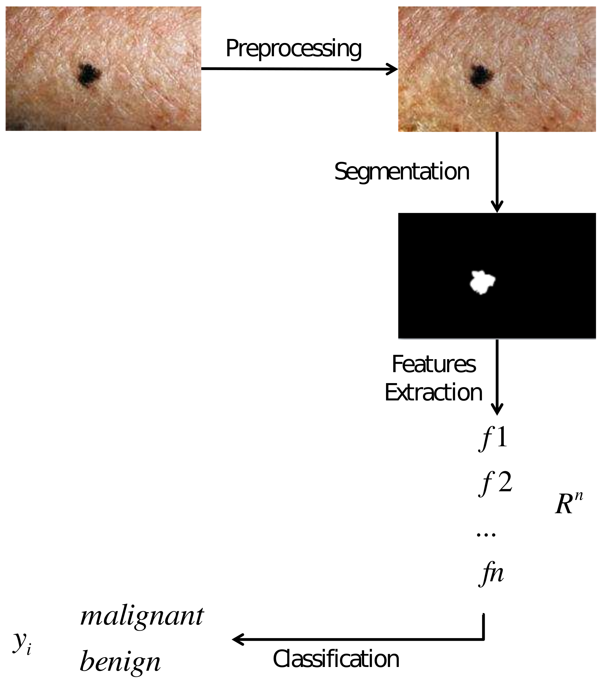
Skin cancer detection involves different stages that include pre-processing, segmentation, feature extraction and classification.
The basic work flow of automatic skin cancer detection is shown in Figure 1.
Details of the phases are as follows.
3.1. Preprocessing
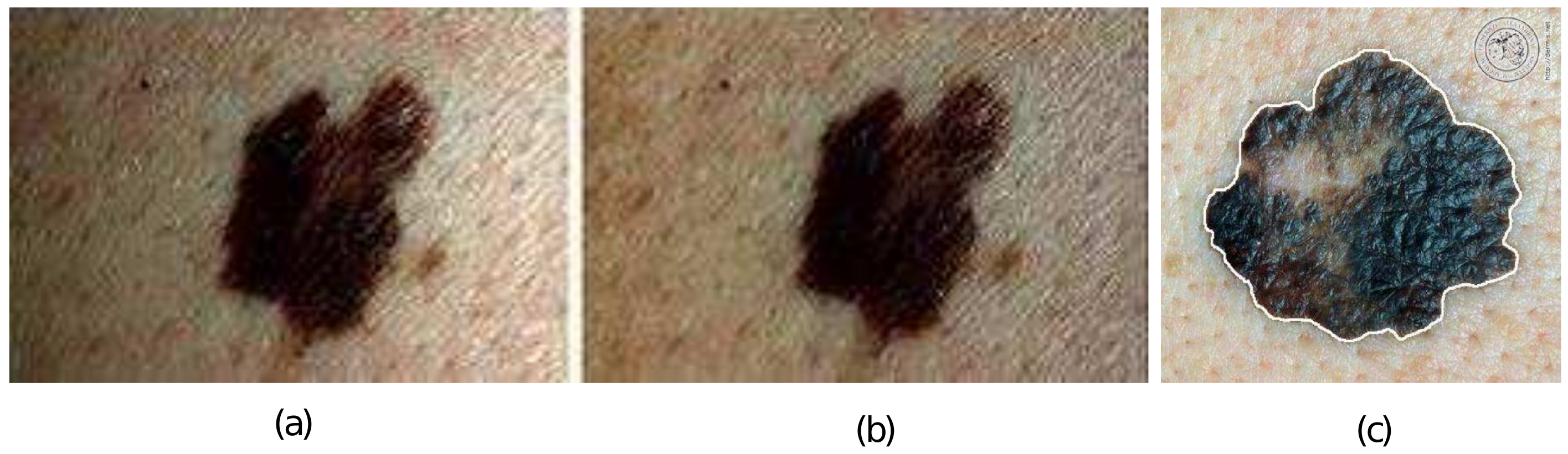
Preprocessing involves illumination correction of the images found in the data-set. Purpose of illumination correction is to standardize lighting exposure across the entire image. Accuracy of features depend upon pixel values, which in turn depends upon the illumination correction. In general, pre-processing can not be restricted to the lighting problem or illumination correction alone but seen in a realistic way. Indeed, image pre-processing is an essential step of detection in order to remove noises and enhance the quality of the original image [42,43,44]. Figure 2a,b show the original image and the one after pre-processing respectively, as discussed in [3].
Using the multistage illumination modeling algorithm, the first stage is to estimate the illumination map of the image using Monte Carlo and then the parametric modeling strategy is incorporated into the second stage to estimate the final illumination map.
3.2. Segmentation
Segmentation characterizes the image pixels into semantic groups. In case of skin cancer detection, segmentation extracts the lesion border that separates it from the surrounding non-cancerous tissues. The result of segmentation is a binary mask at the location of lesion. Figure 2c shows the segmentation of skin lesion. A variety of segmentation strategies have been used for skin lesion detection. Lynn et al. [45] used the mean shift segmentation method to separate skin lesion from background image pixels. Adjed et al. [46] used generalization of the Chen and Vese model for segmentation of skin lesion. Nammalwar et al. [47] used combined color and texture features for segmentation of skin cancer images. Sumithra et al. [48] used a region growing method with initialization of seed points for segmentation. In our project, we have used an already manually segmented dataset of images acquired from the University of Waterloo.
3.3. Feature Extraction
Feature extraction involves specific predefined calculations on the preprocessed and segmented image. In this process, feature vectors of important characteristics of an image are generated. The features are then used to separate malignant from benign cases. Rashi et al. [49] used GLCM parameters as the skin cancer detection features and the SVM classifier for classification. They also used GLCM parameters, with the back propagation neural network as the classifier. For skin cancer, GLCM parameters and color features of the image bear important information and were explored for this project.
3.3.1. Gray Level Co-occurrence Matrix (GLCM) and Haralick’s Statistical Texture Descriptors
The Gray Level Co-occurrence Matrix (GLCM) can be used to evaluate the texture of an image. The relationship between the pixels having different gray levels is represented by GLCM. For this purpose, a separate matrix is generated for each set of pixel offset and orientation. Haralick proposed second order statistical texture descriptors that can be determined from the GLCM.
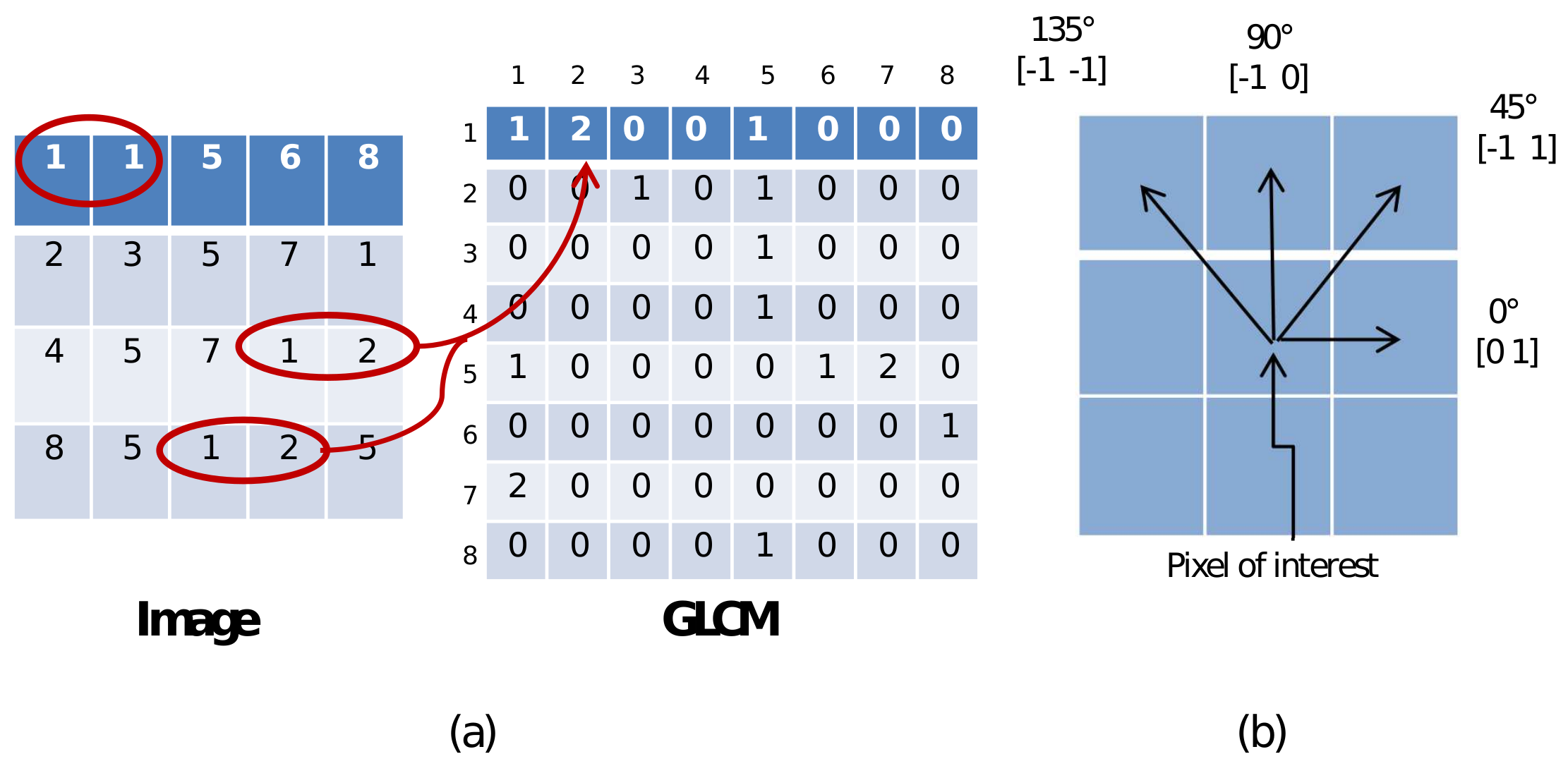
In our research, we used four GLCM parameters i.e., energy, homogeneity, correlation and contrast. These parameters are found by using MATLAB function graycomatrix (R2017a, MathWorks, Natick, Massachusetts, USA). A GLCM contains the information about frequency of gray level repetition for a certain offset distance between two pixels and a certain orientation with respect to each other. The default number of gray levels used by the function is eight. GLCM is demonstrated graphically with Figure 3a. The figure contains an image referenced I, with dimensions . As the total number of gray levels in the image is 8, a GLCM matrix with dimension is used to represent the relationship of gray levels between the pixels. Each coordinate pair of GLCM matrix represents gray levels of the two pixels separated by a certain offset and positioned at a certain angle. Thus, in a cell of GLCM, the row number represents the gray level of the first pixel and the column number represents the gray level of the second pixel in the pair. The content of a GLCM cell shows how frequently the pixel pairs corresponding to that cell appear in the image. In this figure, Image I contains a single pair of gray level (1,1) so the corresponding spatial coordinate of GLCM (at row 1 and column 1) contains a 1. There are two instances of the pair with pixel values 1 and 2, so the cells in row 1 and column 2 contain 2. A similar relationship holds for all the elements of the GLCM matrix and the gray level pairs of the image.
The convention used for the pixel distance with respect to the reference pixel is that it increases towards the right as the number of columns increases and downwards as the number of rows increases. If the offset is 1 and angle is 0 degrees, then the pixel is at position (0,1) relative to the reference pixel, as they are in the same row but adjacent columns. For images containing heterogeneous texture, GLCM with different offsets and orientations are required and analyzed, to cater for the statistics with different offsets and orientations. In general, the offset pairs have the following meaning and are shown in Figure 3b. , where D is the distance between the two pixels. In our research, we have used four, second order statistical descriptors i.e., contrast, correlation, homogeneity and energy with a certain offset and four different angles to classify between melanoma and non-melanoma. MATLAB function graycoprops is used for this purpose. Haralick [50] proposed many GLCM parameters, but we used the ones discussed above for skin cancer detection, as they have shown very good results in the past [9,51]. A part of the samples is used for training while the remaining is for testing the trained ANN.
The four statistical parameters that were discussed above are explained below.
Contrast measures the spatial frequency of an image. It is the difference in the moment of GLCM. Contrast is the difference between the highest and the lowest values of a contiguous set of pixels. It actually measures the amount of local variations present in the image:
Energy is the sum of squared elements in the GLCM matrix. It is also called Uniformity or Angular second moment:
Homogeneity is a measure of how close is the distribution of elements in GLCM to its diagonal. It is also called Inverse Difference Moment. If all the elements are the same, homogeneity attains a maximum value:
Correlation is a measure of how correlated a pixel is to its neighboring pixels over the whole image. It is a measure of gray tone linear dependencies in the image:
where and are the means and standard deviations of and .
3.3.2. Color Features
For skin cancer detection, color features bear useful information and were used for this project. A color image is divided into three color planes i.e., red, green and blue. Statistical features of mean, median and standard deviation were extracted for each color plane. These features can be expressed as follows:
Mean is the average value and is computed as the sum of all the observed outcomes from the sample, divided by the total number of events:
where x is the observed outcome and n is the total number of events.
Median is the middle value of the list after all the outcomes from the samples are sorted.
3.3.3. ABCD Features
These are the features that dermatologists commonly use. The significance of these features is that, based on them, a dermatologist decides whether an observed skin lesion is a melanoma or not. The ABCD rule followed by the doctors has been mathematically modeled and implemented in this project. The details of these features are as follows:
Asymmetry is an important feature for detection of skin cancer. It is represented in terms of Asymmetry Index. In order to find this feature, it is necessary to find the true axis of symmetry around which the image of lesion area is folded. This was done by first finding the center of rotation of the image. The center of image is taken as the point placed in the middle row and middle column of a rectangular region that encompasses the image. The image is then folded at different axes, each passing through the center. A total of 18 axes at increments of , for a total of , were tried. The true axis of symmetry is the one at which the two halves, when folded, result in maximum overlap. The asymmetry index is defined in Equation (7):
where A is the total area of the lesion and is the difference in area of the two halves of the folded region i.e., non-overlapping region.
Border Irregularity: Another important feature for the identification of melanoma or non-melanoma is the shape of the lesion. A regular border is usually benign while an irregular border indicates melanoma. Equation (8) shows border irregularity by using Compactness Index as follows:
where is perimeter of the segmented lesion region and is its total area.
Color: It is the most important feature in melanoma and can be identified by using the statistical features i.e., mean, median and standard deviation of each plane (red, green and blue).
Diameter: The main feature that has been often ignored is the diameter. Diameter changes with distance between the capturing device and the lesion. For fair comparison, the distance between camera and the lesion should remain the same for all images in a data-set. In our research, instead of using diameter, we have introduced a new feature i.e., Oblongness, which is the ratio of length and width. Here, length is the same as the usual diameter feature and is taken along the true axis of symmetry; and width is taken along the axis perpendicular to it, passing through the center of true axis of symmetry. Thus, regardless of distance and orientation of the capturing device, the ratio remains the same.
3.4. Classification
The last stage of automatic skin cancer detection is classification. Classification involves assigning label to the image, based on the feature vector. Skin cancer detection involves supervised learning in which labels of the extracted feature vector are already known. The classification problem consists of two steps: training and testing. In training, the feature vector is applied as an input to the classifier and the corresponding labels form the target outputs. The classification scheme then learns the mapping for separating the two classes from each other. In the testing step, new image features are applied to the trained network which then estimates the image class.
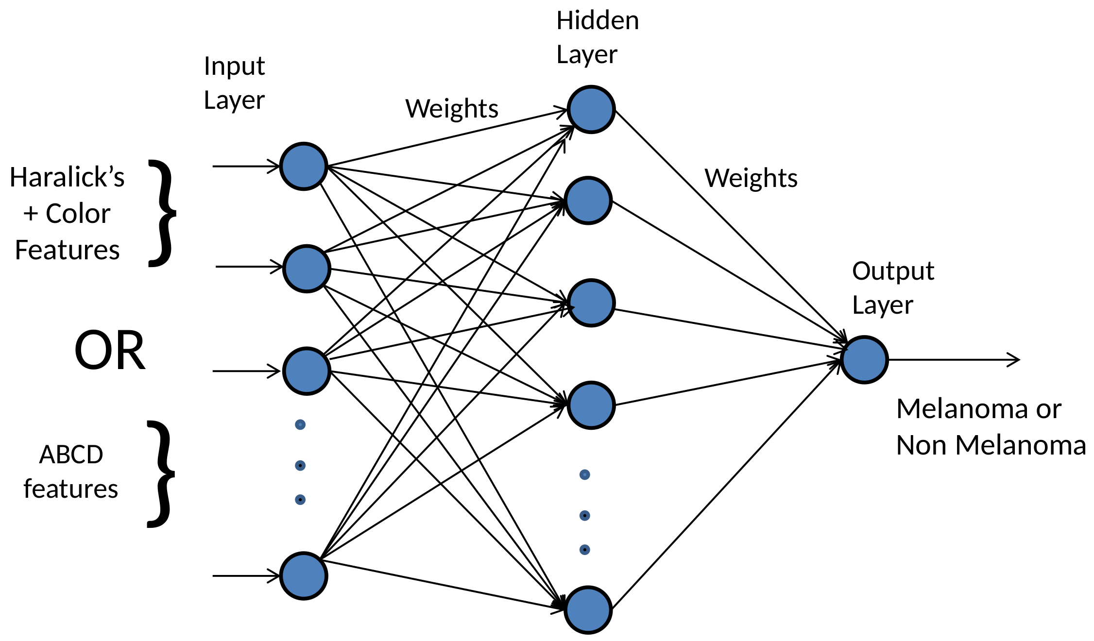
Artificial Neural Networks (ANN) have been used for decades to solve real world problems, especially in the domain of image processing. Here, ANN classifies a skin lesion into melanoma or non-melanoma. We used the feedforward multilayer neural network. The architecture of ANN is comprised of 12 input nodes and a single hidden layer with 15 neurons. Such setup is feasible for our application. Furthermore, we have tested it for a varying number of hidden layers and the number of neurons per layer. However, we achieved the best performance for a single hidden layer with 15 neurons and an input of 12 nodes.
In order to train the network, the back propagation BP algorithm was used. In a multilayer neural network, there is one input layer and at least one hidden layer and one output layer. The hidden and the output layers take part in adjusting the weights that depend on the classification error. The signal flows in the forward direction and the error is back propagated to update the weights. This results in the reduction of error calculated through the difference between the actual and target output. Initial weights of the neural network are considered at random. This technique in which the network is trained by reducing the difference between the actual and target outputs is also called supervised learning.
The output is generated by applying the input to the initial weights and the activation function. The actual output so produced is compared to the target output and the weights updated in order to reduce the difference. This process continues until there is zero error or the number of epochs reach a preset value. After training, the network is tested with new data for classification accuracy. A ‘0’ at the neural network output indicates a non-cancerous or non-melanoma case, while a ‘1’ indicates cancerous or melanoma cases. Figure 4 shows a typical ANN.
3.5. Selection of the Number of Hidden Nodes
Although we are not aware of a well-established theory regarding the number of hidden neurons in the hidden layer, there are empirical rules (rule-of-thumb) that have been proposed in the literature. Having too few neurons in the hidden layer leads to under-fitting, whereas having too many neurons will lead to over-fitting where the network will essentially memorize the input samples and does not generalize well to the new test data. In general, the number of hidden layer neurons should be (a function of) between the size of the input and output layers and are usually selected through cross validation to ensure the network is not over-fitting to the training data.
In general, an exhaustive search is used to find an optimal ANN architecture for better performance. However, the mathematical relationship for computing hidden neurons with respect to the number of input node, input samples, number layers and output nodes have been investigated in the literature that can provide a good set of initial parameters to evaluate an ANN performance.
As such, Santin et al. [53] design, train and test 4000 neural networks with different architectures for the problem of estimating riparian buffer width. They have used nine different neural network architectures with an input-hidden-output configuration of to . An individual architecture produces five different neural networks initialized with different weights and biases. Furthermore, 100 different training sets are produced in order to generate different neural network configurations. The basic architecture is to . However, the configuration of ANN architecture used in our research is , which almost resembles one of the architectures used by Santin et al. i.e., in [53] with the input to a hidden neurons relationship.
Sheela et al. [54] provide a review on various methods to fix the number of neurons in relation to the number of inputs and outputs. Devi et al. have used an optimum number of hidden neurons by the trial and error technique [55]. Xinzhe [56] have proposed and used a formula to test 40 cases, where is number of hidden nodes. is number of input nodes, is number of input samples and L is the number of hidden layer. In our case, , and produce the number of hidden nodes, . Nonetheless, we have used 15 hidden nodes which are lesser than the one computed through formula investigated by [56]. The method described by Trenn [56] is , where is the number of hidden nodes, n is the number of inputs and is the number of outputs. According to this method, the number of hidden nodes compute to be or if rounded , which is almost the same as we investigated in our research with original .
3.6. Input Samples to Number of Hidden Nodes
In our case, a mathematical relationship to compute the number of hidden nodes with respect to the number of input and output nodes is , where is the number of hidden nodes and is the number of output nodes. and , which results in 15. Similarly, a mathematical relationship to compute number of hidden nodes with respect to the number of input nodes and the number of input samples is , where is number of input samples and is equal to 206, which computes out to be and if rounded becomes 15 nodes.
4. Implementation Details
Automatic skin cancer detection is divided into different modules. The modules are generated in MATLAB. These include image acquisition, computing region of interest (ROI) and feature extraction. In the image acquisition stage, two popular data-sets of DermIS and Dermquest were used for dermoscopic images and manually segmented lesions. These data-sets contain cases for both melanoma and non-melanoma. Total number of samples in these data-sets is 206, out of which 119 samples belong to melanoma and 87 samples to non-melanoma type. From a segmented lesion, the region of interest (ROI) is determined by finding the minimum and maximum row and column indices of the segmented image. Once ROI is extracted, it is used for further processing. From the ROI image, a GLCM is produced. From the GLCM, four Haralick’s statistical parameters of contrast, correlation, energy and homogeneity are extracted, for offsets of and 28; and four different angles i.e., , , and . The parameters are fed as input to the neural network. The neural network is trained and tested with different random seeds and configured with 15 hidden nodes, as shown in Table 1. Training data are taken randomly using different random seeds, and 50%, 70% and 90% of the data set. The results contain the accuracy rate and the confusion matrix. All features except color features are extracted using gray scale images, while color features necessarily require individual color planes. Therefore, we have used gray scale ROI for computation of all features including GLCM, Asymmetry, Border irregularity, diameter and ROI of three color planes for statistical measures of individual colors. Similarly, color features are extracted and applied to the neural network. For extraction of the color features, the ROI is divided into red, green and blue planes. Mean, median and standard deviation are calculated for each plane. Thus, a total of nine color parameters are determined. These features alone and, in combination with GLCM features, are used to find the performance of the neural network in skin cancer detection.
By comparing the average performance values, the best results are obtained with 50%, 25% and 25% for training, validation and test data splits, respectively.
The performance of ANN for cancer detection is evaluated with GLCM parameters determined for different offsets of and 28. The results from Table 2 show that the best performance is obtained with offset = 24. The performance of ANN with ABCD features was also evaluated. We provided an input of twelve features to the ANN including one feature for asymmetry, one pertaining to the border irregularity, nine color features and one for diameter that captures the Oblongness. The ANN is comprised of 15 hidden nodes. The data used were in a split of 70% training set and 30% of test set.
Modified Standard Deviation
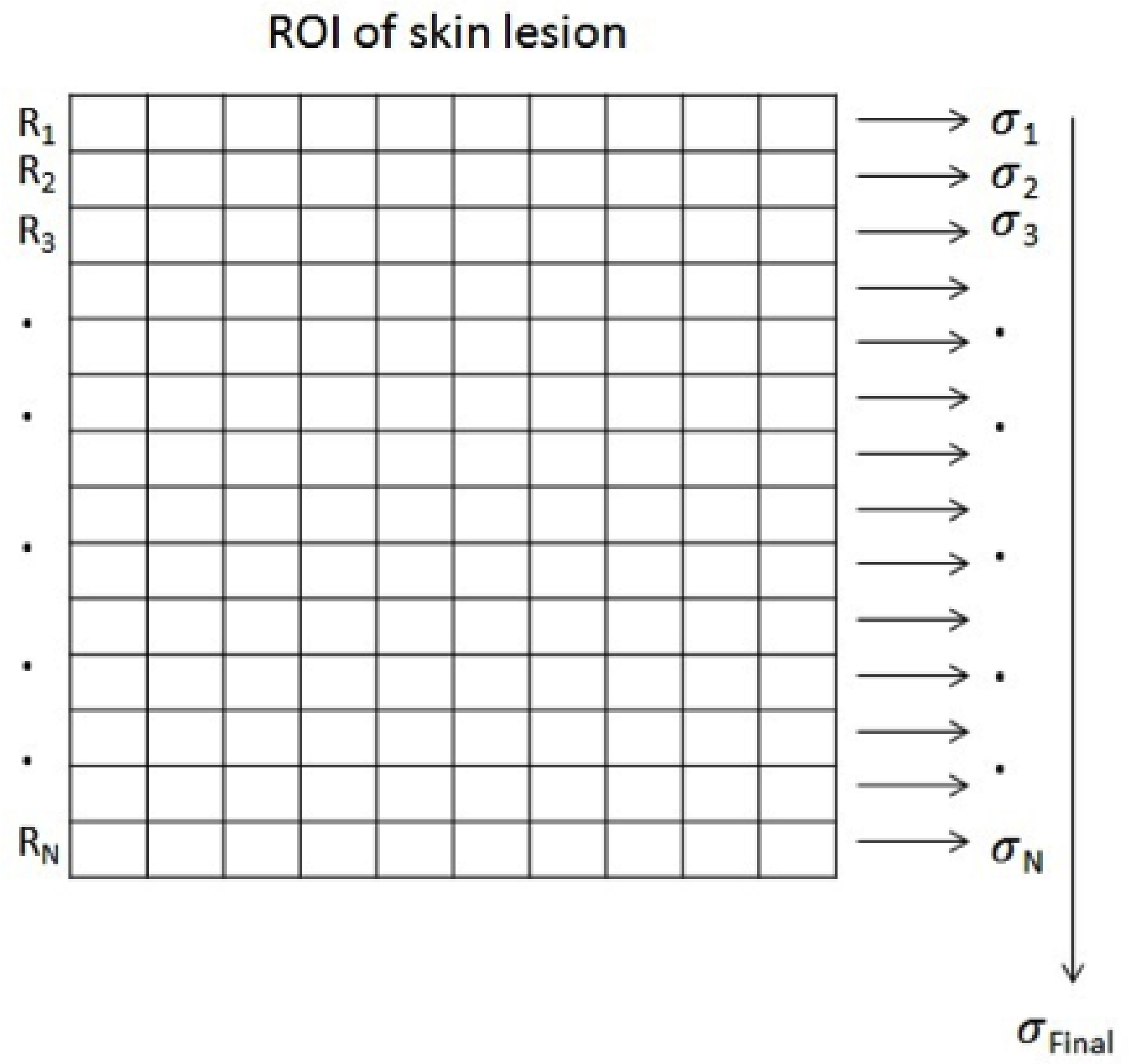
In this research paper, we have proposed a new dimension of finding standard deviation of an image named as modified standard deviation. In this case, the standard deviation is taken row wise and then a column comprising of the resultant standard deviation from each row undergoes the process of computing standard deviation, which results in a single feature value of the standard deviation as delineated in Algorithm 1. As compared to conventional standard deviation, the modified standard deviation results in a different value—much suitable for melanoma classification.
| Algorithm 1 Compute Modified Standard Deviation |
| Input: Image of dimension: Output: Final value of the modified standard deviation, Step 1: Compute standard deviation vector along each row vector from the ROI of an image Step 2: Compute final value of standard deviation along the column vector of standard deviation |
The procedure of finding modified standard deviation is shown in Figure 5. Here, standard deviation of ROI of skin lesion is computed row wise. The result of the row wise standard deviation is again a column vector with each element corresponding to the result of standard deviation for each row. The final value of modified standard deviation is computed along the resultant standard deviation vector. We compute the standard deviation of the column vector again to compute the final feature value. The final result is a single value of the standard deviation, which is attained from the applied ROI on skin lesion image as shown in Figure 5. This proposed way of computing and extracting standard deviation of image results in a different value as compared to the conventional standard deviation comprised of a matrix. Replacing conventional standard deviation features by the modified version of standard deviation outperforms and improves overall results in the ANN classification by 4.23%
5. Evaluation and Results
5.1. Impact of Varying Seed Values on Accuracy
Table 1 shows that the ANN performance by considering as training data, as validation and as verification data. The ANN constitutes from 15 hidden nodes and different random seeds are fed to it. The offset taken in this case is 2 with all the four directions. Sixteen GLCM parameters (four for each one of contrast, energy, homogeneity, and correlation) are used as input to the neural network. Similarly, ANN performance is evaluated by taking as the training data, as validation data and as verification data and by taking as training data, validation and verification data. The best results are shown in bold letters. The average performance is also shown.
In Table 1, it can also be seen that insufficient and uneven availability of dataset may result in varying accuracy. Number of images used for classification can adversely affect the accuracy. Recent work shows varying success rate with varying number of images as shown by Rashi Goel et al. [49] for multiclass skin cancer disease. The random seeds select different combination of samples in the dataset for training, test and validation, which shows that dataset used in training have an impact on computing the final accuracy of the classifier. Alternatively, the best result shows the best set of training samples. The true representative of data and large dataset can result in further improvement in the accuracy of classifier.
From Table 1, it is clear that, on average, choosing 50% training data gives better results and within 50% percentage for selecting training dataset, random seed = 8.15 × 10⁵ selects the best training subset. Furthermore, offset taken here is an initial offset without digging into other options for better offsets, and is used for evaluating the best distribution of dataset in the percentage for training, testing and validation using a random seed generated in MATLAB.
5.2. Impact of Offset Selection on Accuracy
In Table 2, further analysis is done to choose an optimal offset that gives best results along with best outcomes from Table 1. In Table 3, different feature set is used for analysis using the mean, median and SD of each of red, green and blue planes, best results are found by using 50% and 70% training data.
5.3. Performance of GLCM, Statistical Features and ABCD Features
Table 4 shows the results of using another feature set which is a combination of GLCM and the red, green and blue statistical or low-level intuitive features including mean, median and standard deviation. Here, the total number of inputs is 25, out of which 16 features are extracted from GLCM and 9 features are mean, median and standard deviation for each of the red, green and blue planes of ROI. The best result found is by using training data, validation and 15% verification data. Table 5 shows the classification results of ANN with ABCD features which are HLIF. Here, features are asymmetry, border irregularity, color features including mean, median, standard deviation for red, green, blue planes and diameter which depicts oblongness. It can be seen that accuracy as high as is achieved with these features. Here, results are generated using of training dataset.
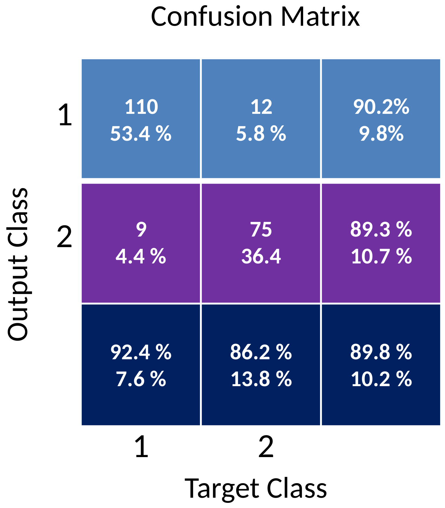
It is clear from our experiments that most of the results using 70% of the training set are better than other data split and it is also most a common practice to split data into 70%:30% of training:test set. The accuracy found by using (ABCD) HLIF are comparable to the methods found in the literature. The confusion matrix is shown in Figure 6. At the end, we analyze the performance of ANN through the fusion of GLCM and ABCD features with expectations of getting higher accuracy, but the results are not promising. The accuracy found through fusion of ABCD and GLCM is .
5.4. Impact of Modified Standard Deviation
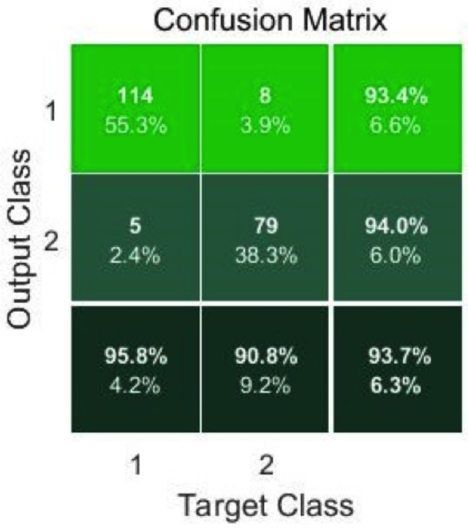
Furthermore, results of ABCD are computed using modified standard deviation. In color features of ABCD, conventional standard deviation of each color plane of ROI is replaced with modified standard deviation and classification is done using ANN. Replacing conventional standard deviation with modified standard deviation results in improvement in accuracy from to . Our main goal is to provide melanoma detection scheme, with best features selection and classification using ANN. Our proposed modified standard deviation has improved accuracy by . Moreover, sensitivity and specificity are and , respectively. The confusion matrix of using proposed modified standard deviation is shown in Figure 7.
In addition to that, the experiments are performed with an increased number of hidden layers and neurons. We observe that the accuracy does not improve further as compared to using 15 hidden neurons with 12 inputs of ABCD. The experiments with a varying number of hidden layers, number of neurons and the corresponding accuracy is captured in Table 6.
5.5. Comparison with State-Of-The-Art
In our proposed method, some of the features are the same as compared to [57]. The performance in the [57] is computed with the features mentioned along with GLCM parameters. In our paper, we also combined ABCD features with GLCM parameters, but there is no further improvement in results as compared to using ABCD features alone. However, accuracy achieved by coupling GLCM and ABCD features with modified standard deviation is .
The number of images used in [31] is 200 images, while in our paper we used 206 images. The number of images used in both papers is the same, but the datasets are different. In the referenced work, Interactive Atlas of Dermoscopy and a private dataset is used, while we have used the DermIS and DermQuest dataset.
The classification is done using SVM after applying the correlation based feature selection (CFS) algorithm, while we used ANN directly applied on the features extracted.
The performance is better in terms of sensitivity and comparable results in terms of specificity. Sensitivity in the [31] is 90%, while in our proposed method the sensitivity found is 95.8%. Specificity in previous work is 96%, while, in our proposed method, it is 91%. The accuracy is not mentioned in the above-mentioned work; however, we achieve an accuracy of 93.7%.
The bottom line is that, in both of the papers, ABCD features are incorporated. In [31], a subset of ABCD features is combined with GLCM parameters along with the CFS algorithm to select features. In contrast, we used a complete set of ABCD features with GLCM parameters, although the performance is not significant. Our proposed method is better in terms of the number of selected features, i.e., no further feature selection processing on the extracted features and in terms of better sensitivity and accuracy with approximately the same number of images.
6. Discussion
Skin cancer is one of the most common types of cancer. Melanoma is the deadliest type of skin cancers. Automatic skin cancer detection is needed to help physicians for early detection. In this research, automatic detection of skin cancer was done with a comparison analysis of high level and low level intuitive features. Neural networks were used for classification. Results were generated for GLCM parameters with different offsets in the range of 2–28 and the offset that gave the best result was chosen. Color features were also used to check the performance of neural networks. Results were comparable to those obtained with the GLCM parameters. A combination of GLCM parameters and color features applied to ANN resulted in even better performance. Finally, ABCD features in which color parameter has the same statistical measures of color planes and diameter was replaced with oblongness resulted in the highest accuracy. Color features outperform in both cases when combined with GLCM and ABCD.
Table 7 shows performance results of the proposed method compared to the methods adapted by contemporary researchers. One of the big challenges in medical image analysis research is the non-availability of large datasets. Table 7 shows that different datasets are used by different researchers and even the amount of data used is different. Each accuracy shown is true with respect to its own experimental setup and data used, but we cannot say it as true accuracy among different researchers. True accuracy among different research studies should be conducted with same platform, equal amount of data and the same dataset for finding performance of skin cancer detection.
Brinker et al. [58] also commented on performance comparison of skin cancer related research due to use of non-public datasets and recommended to use publicly available benchmark datasets. The second challenge is uneven dataset of class melanoma and non-melanoma cases that can affect accuracy. The third challenge is the choice of dataset used for training as it is confirmed by our experiments that, different random seeds come up with different accuracy with the same experimental setup. ANN with an increasing number of hidden layers with different numbers of nodes can also affect accuracy. Conversely, a higher number of hidden layers can increase the computation cost.
High-level intuitive features ABCD give better performance in terms of accuracy and with a reduced number of features i.e., 12 inputs to ANN. The results are derived on publicly available datasets of DermIS and DermQuest with 206 images. The dataset used in literature as stated in Section 2 in [31] is identical to the one used in our research paper, i.e., DermIS and DermQuest with the same number of images i.e., 206. In [31], they found and of sensitivity, specificity and accuracy, respectively. As compared to the referenced paper, our method results in and sensitivity, specificity and accuracy, respectively. Our results are better i.e., accurate as compared to the [31].
Part of the reason for better performance is the use of ABCD features with less extracted features fed to the most suitable neuron size of artificial neural networks. In [31], they have used a total of 59 features in their results and did not apply any features’ reduction steps. In contrast, our feature set is comprised of only 12 features, which is very compact as compared to 59. Therefore, the performance achieved is not only better in terms of accuracy, but also in terms of a reduced number of features as compared to the same dataset used in the literature.
7. Conclusions and Future Directions
In order to decrease mortality rate through early detection of melanoma and providing an aid to doctors, image features were extracted, analyzed and classified using ANN. The combination of GLCM and color features gave better results as compared to using these features standalone. Another set of features i.e., ABCD were also applied to ANN and its results were found to be the best of all the tests performed with the other features, with an accuracy of . Both the sets contain color features showing its significance for the detection of skin cancer. In ABCD features, diameter is usually ignored because different orientations of the capturing device result in different diameters. We introduced a new feature, Oblongness in place of Diameter that considers the ratio of length and width, with the length taken along the true axis of symmetry. In the future, we intend to work on skin cancer detection using deep learning and evolutionary algorithms. Moreover, we would like to perform research work on a publicly available large database of ISIC (International Skin Imaging Collaboration) for skin cancer detection [60]. In order to compute the true accuracy and comparable results, researchers must be provided with an identical platform, big data, and the same number of image samples with common training and test datasets. In the future, we intend to develop an end-to-end PC-based detection system that would be capable to analyze a lesion in real time, using a camera attached to the PC.
Author Contributions
M.A. and N.M. worked on the conceptualization and methodology. M.A. and A.H. worked on software, formal analysis and validation. A.M.A. worked on the methodology. A.S. and Z.U. helped in writing and editing the original draft. N.M., Z.U. and A.H. supervised the project and the administration.
Funding
The financial support of National Center of Big data and Cloud Computing—NCBC, University of Engineering and Technology, Peshawar, under the auspices of Higher Education Commission, Pakistan, is gratefully acknowledged.
Conflicts of Interest
The authors declare no conflict of interest.
Abbreviations
The following abbreviations are used in this manuscript:
| ANN | Artificial Neural Network |
| GLCM | Gray Level Co-occurrence Matrices |
| ABCD | Asymmetry Border irregularity Color Diameter |
| HLIF | High Level Intuitive Features |
| LLIF | Low Level Intuitive Features |
References
- Guy, G.P., Jr.; Thomas, C.C.; Thompson, T.; Watson, M.; Massetti, G.M.; Richardson, L.C. Vital signs: Melanoma incidence and mortality trends and projections—United States, 1982–2030. MMWR. Morb. Mortal. Wkly. Rep. 2015, 64, 591. [Google Scholar] [PubMed]
- Guy, G.P., Jr.; Machlin, S.R.; Ekwueme, D.U.; Yabroff, K.R. Prevalence and Costs of Skin Cancer Treatment in the US, 2002–2006 and 2007–2011. Am. J. Prev. Med. 2015, 48, 183–187. [Google Scholar] [CrossRef]
- Glaister, J.; Amelard, R.; Wong, A.; Clausi, D.A. MSIM: Multistage illumination modeling of dermatological photographs for illumination-corrected skin lesion analysis. IEEE Trans. Biomed. Eng. 2013, 60, 1873–1883. [Google Scholar] [CrossRef] [PubMed]
- Geller, A.C.; Swetter, S.M.; Brooks, K.; Demierre, M.F.; Yaroch, A.L. Screening, early detection, and trends for melanoma: Current status (2000–2006) and future directions. J. Am. Acad. Dermatol. 2007, 57, 555–572. [Google Scholar] [CrossRef] [PubMed]
- Braun, R.P.; Rabinovitz, H.S.; Oliviero, M.; Kopf, A.W.; Saurat, J.H. Dermoscopy of pigmented skin lesions. J. Am. Acad. Dermatol. 2005, 52, 109–121. [Google Scholar] [CrossRef] [PubMed]
- Amelard, R.; Wong, A.; Clausi, D.A. Extracting high-level intuitive features (HLIF) for classifying skin lesions using standard camera images. In Proceedings of the 2012 Ninth Conference on Computer and Robot Vision (CRV), Toronto, ON, Canada, 28–30 May 2012; pp. 396–403. [Google Scholar]
- Rani, N.; Nalam, M.; Mohan, A. Detection of Skin Cancer Using Artificial Neural Network. IJIACS 2014, 2, 20–25. [Google Scholar]
- Ouahabi, A. Signal and Image Multiresolution Analysis; John Wiley & Sons: Hoboken, NJ, USA, 2012. [Google Scholar]
- Jaleel, J.A.; Salim, S.; Aswin, R. Computer Aided Detection of Skin Cancer. In Proceedings of the 2013 International Conference on Circuits, Power and Computing Technologies (ICCPCT), Nagercoil, India, 20–21 March 2013; pp. 1137–1142. [Google Scholar]
- Meriem, D.; Abdeldjalil, O.; Hadj, B.; Adrian, B.; Denis, K. Discrete wavelet for multifractal texture classification: Application to medical ultrasound imaging. In Proceedings of the 2010 IEEE International Conference on Image Processing, Hong Kong, China, 26–29 September 2010; pp. 637–640. [Google Scholar]
- Ouahabi, A. Multifractal analysis for texture characterization: A new approach based on DWT. In Proceedings of the 10th International Conference on Information Science, Signal Processing and their Applications (ISSPA 2010), Kuala Lumpur, Malaysia, 10–13 May 2010; pp. 698–703. [Google Scholar]
- Ouahabi, A.; Femmam, S. Wavelet-based multifractal analysis of 1D, and 2D, signals: New results. Analog Integr. Circuits Signal Process. 2011, 69, 3–15. [Google Scholar] [CrossRef]
- Gerasimova, E.; Audit, B.; Roux, S.G.; Khalil, A.; Gileva, O.; Argoul, F.; Naimark, O.; Arneodo, A. Wavelet-based multifractal analysis of dynamic infrared thermograms to assist in early breast cancer diagnosis. Front. Physiol. 2014, 5, 176. [Google Scholar] [CrossRef] [PubMed] [Green Version]
- Choudhari, S.; Biday, S. Artificial Neural Network for SkinCancer Detection. Int. J. Emerg. Trends Technol. Comput. Sci. 2014, 3, 147–153. [Google Scholar]
- Aswin, R.; Jaleel, J.A.; Salim, S. Hybrid genetic algorithm—Artificial neural network classifier for skin cancer detection. In Proceedings of the 2014 International Conference on Control, Instrumentation, Communication and Computational Technologies (ICCICCT), Kanyakumari, India, 10–11 July 2014; pp. 1304–1309. [Google Scholar]
- Mhaske, H.; Phalke, D. Melanoma skin cancer detection and classification based on supervised and unsupervised learning. In Proceedings of the 2013 International conference on Circuits, Controls and Communications (CCUBE), Bengaluru, India, 27–28 December 2013; pp. 1–5. [Google Scholar]
- Alfed, N.; Khelifi, F. Bagged textural and color features for melanoma skin cancer detection in dermoscopic and standard images. Expert Syst. Appl. 2017, 90, 101–110. [Google Scholar] [CrossRef] [Green Version]
- Ritesh, M.; Ashwani, S. A Comparative Study of Various Color Texture Features for Skin Cancer Detection. In Sensors and Image Processing; Springer: Berlin, Germany, 2018; pp. 1–14. [Google Scholar]
- Nezhadian, F.K.; Rashidi, S. Melanoma skin cancer detection using color and new texture features. In Proceedings of the Artificial Intelligence and Signal Processing Conference (AISP), Shiraz, Iran, 25–27 October 2017; pp. 1–5. [Google Scholar]
- Kavitha, J.; Suruliandi, A.; Nagarajan, D.; Nadu, T. Melanoma detection in dermoscopic images using global and local feature extraction. Int. J. Multimed. Ubiquitous Eng. 2017, 12, 19–28. [Google Scholar] [CrossRef]
- Kavitha, J.; Suruliandi, A. Texture and color feature extraction for classification of melanoma using SVM. In Proceedings of the 2016 International Conference on Computing Technologies and Intelligent Data Engineering (ICCTIDE’16), Kovilpatti, India, 7–9 January 2016; pp. 1–6. [Google Scholar]
- Almansour, E.; Jaffar, M.A. Classification of Dermoscopic skin cancer images using color and hybrid texture features. IJCSNS Int. J. Comput. Sci. Netw. Secur. 2016, 16, 135–139. [Google Scholar]
- Adjed, F.; Gardezi, S.J.S.; Ababsa, F.; Faye, I.; Dass, S.C. Fusion of structural and textural features for melanoma recognition. IET Comput. Vis. 2017, 12, 185–195. [Google Scholar] [CrossRef]
- Kolkur, M.S.; Kalbande, D.; Kharkar, V. Machine Learning Approaches to Multi–Class Human Skin Disease Detection. Int. J. Comput. Intell. Res. 2018, 14, 29–39. [Google Scholar]
- Chen, J.; Stanley, R.J.; Moss, R.H.; Van Stoecker, W. Colour analysis of skin lesion regions for melanoma discrimination in clinical images. Skin Res. Technol. 2003, 9, 94–104. [Google Scholar] [CrossRef]
- Lau, H.T.; Al-Jumaily, A. Automatically Early Detection of Skin Cancer: Study Based on Neural Netwok Classification. In Proceedings of the SOCPAR’09. International Conference of Soft Computing and Pattern Recognition, Malacca, Malaysia, 4–7 December 2009; pp. 375–380. [Google Scholar]
- Li, Y.; Shen, L. Skin lesion analysis towards melanoma detection using deep learning network. Sensors 2018, 18, 556. [Google Scholar] [CrossRef]
- Kawahara, J.; Hamarneh, G. Fully Convolutional Neural Networks to Detect Clinical Dermoscopic Features. IEEE J. Biomed. Health Informat. 2018, 23, 578–585. [Google Scholar] [CrossRef]
- Esteva, A.; Kuprel, B.; Novoa, R.A.; Ko, J.; Swetter, S.M.; Blau, H.M.; Thrun, S. Dermatologist-level classification of skin cancer with deep neural networks. Nature 2017, 542, 115. [Google Scholar] [CrossRef]
- Yu, L.; Chen, H.; Dou, Q.; Qin, J.; Heng, P.A. Automated melanoma recognition in dermoscopy images via very deep residual networks. IEEE Trans. Med Imaging 2017, 36, 994–1004. [Google Scholar] [CrossRef]
- Amelard, R.; Glaister, J.; Wong, A.; Clausi, D.A. Melanoma decision support using lighting-corrected intuitive feature models. In Computer Vision Techniques for the Diagnosis of Skin Cancer; Springer: Berlin, Germany, 2014; pp. 193–219. [Google Scholar]
- Codella, N.C.; Nguyen, Q.B.; Pankanti, S.; Gutman, D.; Helba, B.; Halpern, A.; Smith, J.R. Deep learning ensembles for melanoma recognition in dermoscopy images. IBM J. Res. Dev. 2017, 61, 5:1–5:15. [Google Scholar] [CrossRef] [Green Version]
- Haenssle, H.; Fink, C.; Schneiderbauer, R.; Toberer, F.; Buhl, T.; Blum, A.; Kalloo, A.; Hassen, A.B.H.; Thomas, L.; Enk, A.; et al. Man against machine: Diagnostic performance of a deep learning convolutional neural network for dermoscopic melanoma recognition in comparison to 58 dermatologists. Ann. Oncol. 2018, 29, 1836–1842. [Google Scholar] [CrossRef] [PubMed]
- Gal, Y.; Islam, R.; Ghahramani, Z. Deep bayesian active learning with image data. In Proceedings of the 34th International Conference on Machine Learning, Sydney, Australia, 6–11 August 2017; Volume 70, pp. 1183–1192. [Google Scholar]
- Lopez, A.R.; Giro-i Nieto, X.; Burdick, J.; Marques, O. Skin lesion classification from dermoscopic images using deep learning techniques. In Proceedings of the 2017 13th IASTED International Conference on Biomedical Engineering (BioMed), Innsbruck, Austria, 20–21 February 2017; pp. 49–54. [Google Scholar]
- Bi, L.; Kim, J.; Ahn, E.; Feng, D. Automatic skin lesion analysis using large-scale dermoscopy images and deep residual networks. arXiv 2017, arXiv:1703.04197. [Google Scholar]
- Masood, A.; Ali Al-Jumaily, A. Computer aided diagnostic support system for skin cancer: A review of techniques and algorithms. Int. J. Biomed. Imaging 2013, 2013, 323268. [Google Scholar] [CrossRef] [PubMed]
- Xing, Y.; Bronstein, Y.; Ross, M.I.; Askew, R.L.; Lee, J.E.; Gershenwald, J.E.; Royal, R.; Cormier, J.N. Contemporary diagnostic imaging modalities for the staging and surveillance of melanoma patients: A meta-analysis. J. Natl. Cancer Inst. 2011, 103, 129–142. [Google Scholar] [CrossRef] [PubMed]
- Dubois, A.; Levecq, O.; Azimani, H.; Siret, D.; Barut, A.; Suppa, M.; Del Marmol, V.; Malvehy, J.; Cinotti, E.; Rubegni, P.; et al. Line-field confocal optical coherence tomography for high-resolution noninvasive imaging of skin tumors. J. Biomed. Opt. 2018, 23, 106007. [Google Scholar] [CrossRef] [PubMed]
- Xiong, Y.Q.; Mo, Y.; Wen, Y.Q.; Cheng, M.J.; Huo, S.T.; Chen, X.J.; Chen, Q. Optical coherence tomography for the diagnosis of malignant skin tumors: A meta-analysis. J. Biomed. Opt. 2018, 23, 020902. [Google Scholar] [CrossRef] [PubMed]
- Wijesinghe, R.E.; Park, K.; Kim, D.H.; Jeon, M.; Kim, J. In vivo imaging of melanoma-implanted magnetic nanoparticles using contrast-enhanced magneto-motive optical Doppler tomography. J. Biomed. Opt. 2016, 21, 064001. [Google Scholar] [CrossRef]
- Ouahabi, A. A review of wavelet denoising in medical imaging. In Proceedings of the 2013 8th International Workshop on Systems, Signal Processing and their Applications (WoSSPA), Algiers, Algeria, 12–15 May 2013; pp. 19–26. [Google Scholar]
- Hoshyar, A.N.; Al-Jumaily, A.; Hoshyar, A.N. The beneficial techniques in preprocessing step of skin cancer detection system comparing. Procedia Comput. Sci. 2014, 42, 25–31. [Google Scholar] [CrossRef]
- Bakheet, S. An svm framework for malignant melanoma detection based on optimized hog features. Computation 2017, 5, 4. [Google Scholar] [CrossRef]
- Lynn, N.C.; Kyu, Z.M. Segmentation and Classification of Skin Cancer Melanoma from Skin Lesion Images. In Proceedings of the 2017 18th International Conference on Parallel and Distributed Computing, Applications and Technologies (PDCAT), Taipei, Taiwan, 18–20 December 2017; pp. 117–122. [Google Scholar]
- Adjed, F.; Faye, I.; Ababsa, F. Segmentation of skin cancer images using an extension of chan and vese model. In Proceedings of the 2015 7th International Conference on Information Technology and Electrical Engineering (ICITEE), Chiang Mai, Thailand, 29–30 October 2015; pp. 442–447. [Google Scholar]
- Xu, L.; Jackowski, M.; Goshtasby, A.; Roseman, D.; Bines, S.; Yu, C.; Dhawan, A.; Huntley, A. Segmentation of skin cancer images. Image Vis. Comput. 1999, 17, 65–74. [Google Scholar] [CrossRef]
- Sumithra, R.; Suhil, M.; Guru, D. Segmentation and classification of skin lesions for disease diagnosis. Procedia Comput. Sci. 2015, 45, 76–85. [Google Scholar] [CrossRef]
- Goel, R.; Singh, S. Skin Cancer Detection using GLCM Matrix Analysis and Back Propagation Neural Network Classifier. Int. J. Comput. Appl. 2015, 112, 40–47. [Google Scholar]
- Haralick, R.; Shanmugam, K.; Dinstein, I. Texture Features for Image Classification. IEEE Trans. Syst. Man, Cybern. 1973, 3, 610–621. [Google Scholar] [CrossRef]
- Ahmad, A.M.; Khan, G.M.; Mahmud, S.A.; Miller, J.F. Breast cancer detection using cartesian genetic programming evolved artificial neural networks. In Proceedings of the Fourteenth International Conference on Genetic and Evolutionary Computation Conference, Philadelphia, PA, USA, 7–11 July 2012; pp. 1031–1038. [Google Scholar]
- Al Mutaz, M.A.; Dress, S.; Zaki, N. Detection of Masses in Digital Mammogram Using Second Order Statistics and Artificial Neural Network. Int. J. Comput. Sci. Inf. Technol. 2011, 3, 176–186. [Google Scholar]
- Santin, F.M.; Grzybowski, J.M.V.; da Silva, R.V. Application of neural network ensembles to the problem of estimating riparian buffer width as a function of desired filtering properties. In Proceedings of the Ist International Congress of Management Technology and Innovation, Erechim, Brazil, 21–25 September 2015. [Google Scholar]
- Sheela, K.G.; Deepa, S.N. Review on methods to fix number of hidden neurons in neural networks. Math. Probl. Eng. 2013, 2013, 425740. [Google Scholar] [CrossRef]
- Ramadevi, R.; Sheela Rani, B.; Prakash, V. Role of hidden neurons in an elman recurrent neural network in classification of cavitation signals. Int. J. Comput. Appl. 2012, 37, 9–13. [Google Scholar]
- Ke, J.; Liu, X. Empirical analysis of optimal hidden neurons in neural network modeling for stock prediction. In Proceedings of the 2008 IEEE Pacific–Asia Workshop on Computational Intelligence and Industrial Application, Wuhan, China, 19–20 December 2008; Volume 2, pp. 828–832. [Google Scholar]
- Jaworek-Korjakowska, J. Computer-aided diagnosis of micro-malignant melanoma lesions applying support vector machines. BioMed Res. Int. 2016, 2016, 4381972. [Google Scholar] [CrossRef]
- Brinker, T.J.; Hekler, A.; Utikal, J.S.; Grabe, N.; Schadendorf, D.; Klode, J.; Berking, C.; Steeb, T.; Enk, A.H.; von Kalle, C. Skin Cancer Classification Using Convolutional Neural Networks: Systematic Review. J. Med Internet Res. 2018, 20, e11936. [Google Scholar] [CrossRef]
- Ganster, H.; Pinz, P.; Rohrer, R.; Wildling, E.; Binder, M.; Kittler, H. Automated melanoma recognition. IEEE Trans. Med Imaging 2001, 20, 233–239. [Google Scholar] [CrossRef]
- Codella, N.C.F.; Gutman, D.; Celebi, M.E.; Helba, B.; Marchetti, M.A.; Dusza, S.W.; Kalloo, A.; Liopyris, K.; Mishra, N.; Kittler, H.; et al. Skin lesion analysis toward melanoma detection: A challenge at the 2017 International symposium on biomedical imaging (ISBI), hosted by the international skin imaging collaboration (ISIC). In Proceedings of the 2018 IEEE 15th International Symposium on Biomedical Imaging (ISBI 2018), Washington, DC, USA, 4–7 April 2018; pp. 168–172. [Google Scholar]
Figure 1.
The basic work flow of automatic skin cancer detection.

Figure 2.
(a) Original image; (b) image after pre-processing; (c) segmentation of skin lesion.

Figure 3.
(a) Gray Level Co-occurrence Matrix (GLCM) showing the number of occurrences of sets of gray levels of two adjacent pixels in an image; (b) GLCM offset directions represented by pairs of pixels lying at , , and .
Figure 3.
(a) Gray Level Co-occurrence Matrix (GLCM) showing the number of occurrences of sets of gray levels of two adjacent pixels in an image; (b) GLCM offset directions represented by pairs of pixels lying at , , and .

Figure 4.
A typical ANN with Input, Hidden and Output layers and the different input features used in this project.
Figure 4.
A typical ANN with Input, Hidden and Output layers and the different input features used in this project.

Figure 5.
The procedure for modified standard deviation.

Figure 6.
Classification results of ABCD features with conventional standard deviation.

Figure 7.
Classification results of ABCD features using ANN with modified standard deviation.


Table 1.
ANN Performance with an offset of 2 and GLCM parameters. ANN with input nodes = 16, hidden nodes = 15 and output nodes = 2. Result 1 (Training Data = , Validation & Verification Data = ), Result 2 (Training Data = , Validation & Verification Data = ), Result 3 (Training Data = , Validation & Verification Data = ). ANN—Artificial Neural Networks; GLCM—Gray Level Co-occurrence Matrix.
| Random Seeds | Result 1 | Result 2 | Result 3 |
|---|---|---|---|
| 71.40% | 69.90% | 65.00% | |
| 67.50% | 66.00% | 68.90% | |
| 67.50% | 67.50% | 42.20% | |
| 68.90% | 65.50% | 65.00% | |
| 66.50% | 58.30% | 66.50% | |
| 65.00% | 66.00% | 60.70% | |
| 68.40% | 50.00% | 58.30% | |
| 69.40% | 65.00% | 71.40% | |
| 57.80% | 65.50% | 42.20% | |
| 67.00% | 62.10% | 63.10% | |
| Average | 66.94% | 63.58% | 60.33% |
Table 2.
Results of different offsets used with constant random seed = 8.15 × 10⁵ and by taking 50% training and 25% validation and 25% verification.
Table 2.
Results of different offsets used with constant random seed = 8.15 × 10⁵ and by taking 50% training and 25% validation and 25% verification.
| Offset | Performance |
|---|---|
| 2 | 71.4% |
| 4 | 65.0% |
| 8 | 68.0% |
| 12 | 69.9% |
| 16 | 70.4% |
| 20 | 70.9% |
| 24 | 76.2% |
| 28 | 73.8% |
Table 3.
Using color features Mean, Median and Standard Deviation of Red, Green and Blue planes (Seed = 8.15 × 10⁵ and No. of hidden nodes = 15).
Table 3.
Using color features Mean, Median and Standard Deviation of Red, Green and Blue planes (Seed = 8.15 × 10⁵ and No. of hidden nodes = 15).
| Training Data | Validation Data | Verification Data | Performance |
|---|---|---|---|
| 50% | 25% | 25% | 76.2% |
| 70% | 15% | 15% | 76.2% |
| 90% | 5% | 5% | 42.2% |
Table 4.
ANN Performance using GLCM and Mean, Median and Standard deviation of (Red, Green and Blue).
Table 4.
ANN Performance using GLCM and Mean, Median and Standard deviation of (Red, Green and Blue).
| Training Data | Validation Data | Verification Data | Performance |
|---|---|---|---|
| 50% | 25% | 25% | 80.1% |
| 70% | 15% | 15% | 81.6% |
| 90% | 5% | 5% | 58.3% |
Table 5.
ANN performance using ABCD features (Seed = 8.15 × 10⁵ and hidden nodes = 15) compared to conventional and modified standard deviation .
Table 5.
ANN performance using ABCD features (Seed = 8.15 × 10⁵ and hidden nodes = 15) compared to conventional and modified standard deviation .
| Standard Deviation Version | Training Data | Validation Data | Verification Data | Accuracy |
|---|---|---|---|---|
| Conventional 2D stdev | 70% | 15% | 15% | 89.8% |
| Modified stdev | 70% | 15% | 15% | 93.7% |
Table 6.
Performance analysis with varying number of neurons and hidden layers using modified standard deviation. [15 15] denotes two hidden layers with 15 neurons each, while [15 15 15] denotes three hidden layers with 15 neurons each.
Table 6.
Performance analysis with varying number of neurons and hidden layers using modified standard deviation. [15 15] denotes two hidden layers with 15 neurons each, while [15 15 15] denotes three hidden layers with 15 neurons each.
| # Hidden Layers | Neurons per Layer | Sensitivity | Specificity | Accuracy |
|---|---|---|---|---|
| 1 | 15 | 95.8% | 91% | 93.7% |
| 1 | 20 | 88.2% | 62% | 77.2% |
| 1 | 25 | 89% | 77% | 84% |
| 1 | 30 | 84% | 78% | 81.5% |
| 2 | [15 15] | 81.5% | 71.3% | 77.2% |
| 2 | [20 20] | 84% | 60% | 93.8% |
| 2 | [25 25] | 76.4% | 67% | 72.3% |
| 2 | [30 30] | 81.5% | 64.4% | 74.3% |
| 3 | [15 15 15] | 89% | 68% | 80.1% |
| 3 | [20 20 20] | 92.4% | 82.7% | 88.3% |
| 3 | [25 25 25] | 82.3% | 80.45% | 81.5% |
| 3 | [30 30 30] | 73.5% | 89.1% | 82.5% |
Table 7.
Performance comparison between the proposed method and those adapted by other contemporary researchers. Spe: Specificity, Sen: Sensitivity, Acc: Accuracy.
Table 7.
Performance comparison between the proposed method and those adapted by other contemporary researchers. Spe: Specificity, Sen: Sensitivity, Acc: Accuracy.
| Features | Method | Data Source | Samples | Spe | Sen | Acc | Ref |
|---|---|---|---|---|---|---|---|
| 2D wavelets | ANN | Skincancer.org | — | 60–75% | [16] | ||
| melanoma color feature | Color histogram analysis | NY Univ., Dept. Dermatology | 129 melanoma, 129 benign | 88–89% | [25] | ||
| wavelets | 3 layer NN | — | — | 89.90% | [26] | ||
| wavelets | Auto associative NN | — | — | 80.80% | [26] | ||
| Shape and radiometric features | KNN | 5363 | 92% | 87% | [59] | ||
| Proposed method | ANN | Derm IS and DermQuest | 206 | 91% | 95.8% | 93.7% |
© 2019 by the authors. Licensee MDPI, Basel, Switzerland. This article is an open access article distributed under the terms and conditions of the Creative Commons Attribution (CC BY) license (http://creativecommons.org/licenses/by/4.0/).
Share and Cite
MDPI and ACS Style
Ashfaq, M.; Minallah, N.; Ullah, Z.; Ahmad, A.M.; Saeed, A.; Hafeez, A. Performance Analysis of Low-Level and High-Level Intuitive Features for Melanoma Detection. Electronics 2019, 8, 672. https://doi.org/10.3390/electronics8060672
AMA Style
Ashfaq M, Minallah N, Ullah Z, Ahmad AM, Saeed A, Hafeez A. Performance Analysis of Low-Level and High-Level Intuitive Features for Melanoma Detection. Electronics. 2019; 8(6):672. https://doi.org/10.3390/electronics8060672
Chicago/Turabian StyleAshfaq, Muniba, Nasru Minallah, Zahid Ullah, Arbab Masood Ahmad, Aamir Saeed, and Abdul Hafeez. 2019. "Performance Analysis of Low-Level and High-Level Intuitive Features for Melanoma Detection" Electronics 8, no. 6: 672. https://doi.org/10.3390/electronics8060672
Note that from the first issue of 2016, this journal uses article numbers instead of page numbers. See further details here.