Modeling and Analysis of Adaptive Temperature Compensation for Humidity Sensors


Jiangsu Key Laboratory of Meteorological Observation and Information Processing, Nanjing University of Information Science & Technology, Nanjing 210044, China
*
Author to whom correspondence should be addressed.
Electronics 2019, 8(4), 425; https://doi.org/10.3390/electronics8040425
Submission received: 2 March 2019
/
Revised: 5 April 2019
/
Accepted: 8 April 2019
/
Published: 11 April 2019
(This article belongs to the Special Issue Deep Learning Applications with Practical Measured Results in Electronics Industries)
Abstract
:In addition to being sensitive to humidity, humidity sensors with moisture sensitive elements are also sensitive to ambient temperature. The fusion of temperature and humidity data is an effective way to improve the accuracy of humidity sensors. In view of the problem of insufficient adaptive ability and poor universality in the current compensation algorithm, a piecewise processing of measured error at different temperatures by using multiple linear regression is proposed in this paper. The least squares method and back propagation (BP) neural network improved by a genetic simulated annealing algorithm (GSA-BP) were used to compensate the measured humidity data of different temperature ranges. The efficiency of the GSA-BP algorithm was tested, and the compensation function model was established. The compensation accuracy was also compared with the accuracies obtained by other methods. The experimental results show that the adaptive segmentation compensation method can significantly improve the measured error of the humidity sensor over a wide temperature range.
1. Introduction
Automatic weather stations monitor changes in the climate environment in real time. The meteorological sensors are susceptible to ambient influences and their measurement errors exist objectively [1]. Usually, the humidity sensor used in automatic weather stations is a voltage output type polymer film humidity sensitive capacitance sensor, which senses the humidity through the humidity sensitive capacitor and then converts it into a voltage amount by the conversion circuit [2]. The humidity sensitive capacitor is mainly composed of an upper electrode, a humidity sensitive material, a lower electrode and a glass substrate. The humidity sensitive material is a high-molecular-weight polymer with a dielectric constant that changes with the relative humidity of the external environment. In addition to being sensitive to ambient humidity, humidity sensitive materials are also sensitive to temperature. The temperature coefficient is not a constant but a variable. Nonlinear compensation for measured data of the sensor is often required [3,4].
The humidity sensor manufacturer and meteorological calibrator will compensate for the influence of temperature on the measurement results, but the compensation effect is not ideal under low temperature (−20 °C) or high temperature (+50 °C) conditions, and the compensation algorithm is not universal over a wide temperature range. It is important to study an efficient and adaptive compensation method for improving the calibration efficiency.
In recent years, many scholars have compensated sensors using both hardware and software and have achieved some notable results. References 5 and 6 proposed using a conditioning chip and concentric wheatstone bridge circuit to compensate [5,6], but this hardware compensation circuit is subject to electronic components’ temperature drift and process technology constraints, which results in high cost and poor compensation. Software compensation has become a research hotspot because of its low cost, strong applicability and high compensation accuracy. In 2014, reference 7 proposed a combination of hardware and software. The circuit was first designed and compensated by the extreme learning machine (ELM) [7]. The hardware compensation circuit itself would be affected by the ambient temperature, the ELM algorithm easily produced the over fitting problem, and the optimal effect could not be obtained. Reference 8 proposed using principal component analysis (PCA) to improve the back propagation (BP) neural network for nonlinear compensation [8]. PCA was the most widely used method of reducing the dimension and error correction. In practical applications, when gross corruptions existed, PCA could not grasp the real subspace structure of the data well, and the algorithm had no universality. In 2015, reference 9 used a particle swarm optimization (PSO) algorithm to optimize the nonlinear compensation method of the BP neural network. PSO had no crossover and mutation operations [9], and the search speed was fast, but it lacked dynamic speed adjustment and would easily fall into a local extremum. The ability to adapt to ambient temperature was not strong. In 2016, reference 10 proposed using the least squares support vector machine (LS-SVM) to compensate [10]. Compared with the artificial neural network, the LS-SVM could overcome the shortage of long training time and was faster than SVM in solving equations. The solution satisfied the extreme condition, but it could not guarantee that it was a global optimal solution, and there was still the problem of easily falling into a local extremum. All of these compensation methods simply applied an algorithm to the sensor compensation and did not account for the influence of temperature, making the compensation method less adaptive, and making it difficult to guarantee the superiority of the compensation algorithm over a wide temperature range.
In recent years, we have conducted considerable research on the nonlinear compensation of humidity sensors. From 2012 to 2017, we proposed an improved BP neural network nonlinear compensation method, which used a genetic algorithm (GA) to optimize the weight and threshold [11,12]. The method avoided the BP neural network plunging into a local extremum, but the compensation speed was slow when the amount of humidity data was large. Furthermore, combined with the influence of temperature on the humidity sensor, a method of segmentation compensation was proposed, and the compensation speed was fast [13], but the segmentation node was artificially selected. The intelligence and adaptive ability were not high. On the basis of our previous research, and inspired by the idea of a multi-information approach, this paper proposes an adaptive nonlinear compensation method for humidity sensors. According to the influence regularity of temperature on humidity sensors, the sensor was compensated by adaptive segmentation, and the effects of various compensation methods were compared and studied.
2. Principle of Compensation
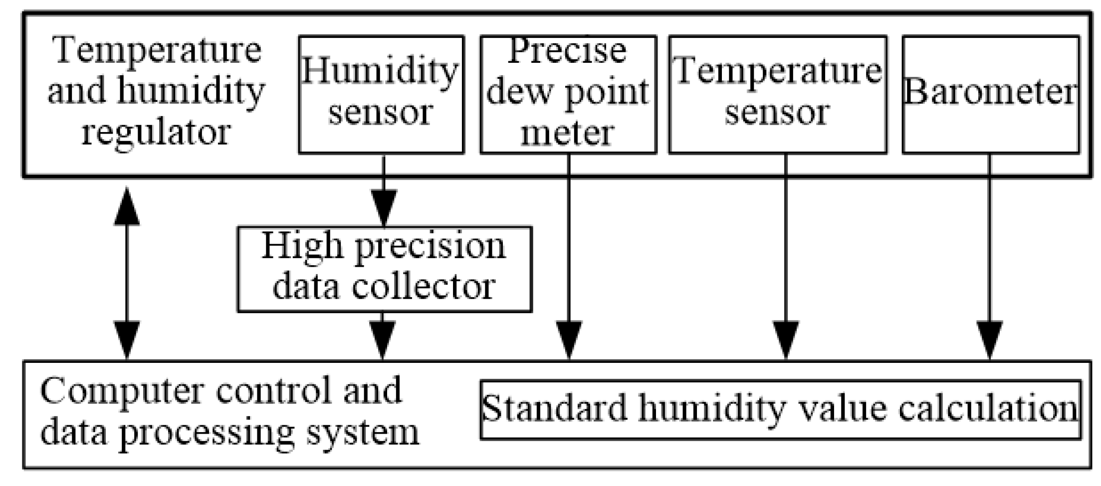
Through a large number of experimental tests, the measured error of the humidity sensor has been shown to be linear near room temperature and nonlinear at high and low temperatures. Some sensors are also nonlinear near room temperature. In the experiment, the humidity sensor was put into the temperature and humidity test chamber, which can adjust the temperature and humidity simultaneously. The standard humidity value was calculated from the measured values of the precise dew point instrument, temperature sensor and pressure gauge. The temperature at which the water vapor in the air becomes dewdrops is called the dew point temperature. The dew point temperature is a means of expressing air humidity. The standard humidity value can be calculated by the experimentally measured dew point value, temperature value and pressure value. In this experiment, the data acquisition range of the data collector was 0.1 uV–100 V, the sensitivity was 100 nV, and the error was ±0.002%. The temperature was measured by a second-class standard PT100 temperature sensor with an allowable error value of ±0.15 °C. During the experiment, all equipment and instruments were verified with high measurement accuracy and could obtain accurate, scientific and reasonable data. The measured value of the humidity sensor was read by the high precision data acquisition unit. The temperature and humidity test chamber was adjusted, and the points near the preset value were observed and recorded. The experimental principle is shown in Figure 1.
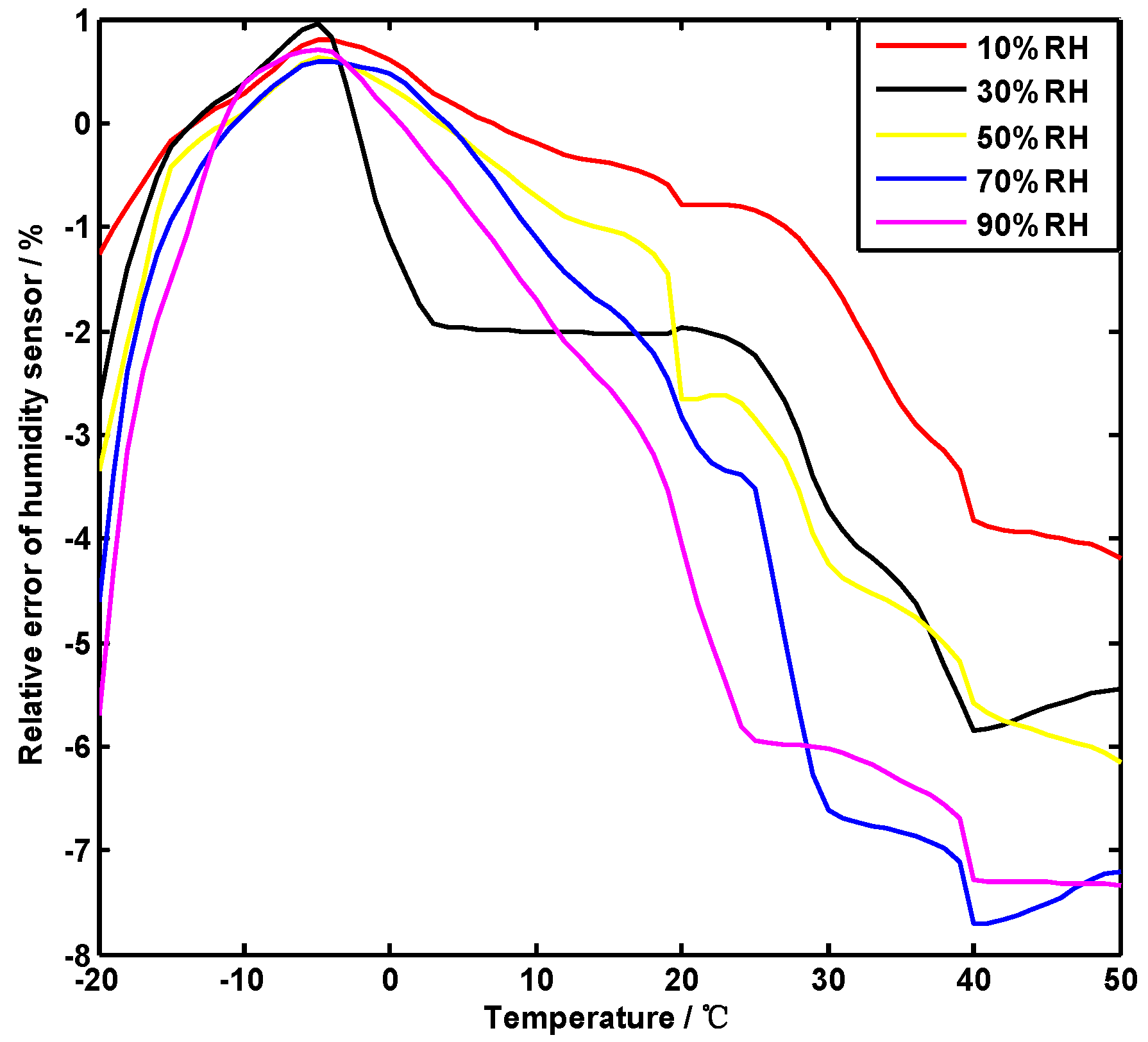
The humidity-sensitive capacitive sensor was placed in the temperature and humidity regulating chamber. The humidity was set to 10% RH, and the temperature was changed. After the temperature was stabilized, the measured value of the humidity sensor was read. The humidity was set to 30% RH, 50% RH, 70% RH and 90% RH, and the above steps were repeated. The measuring error curve of the humidity sensor at different temperatures was obtained as shown in Figure 2.
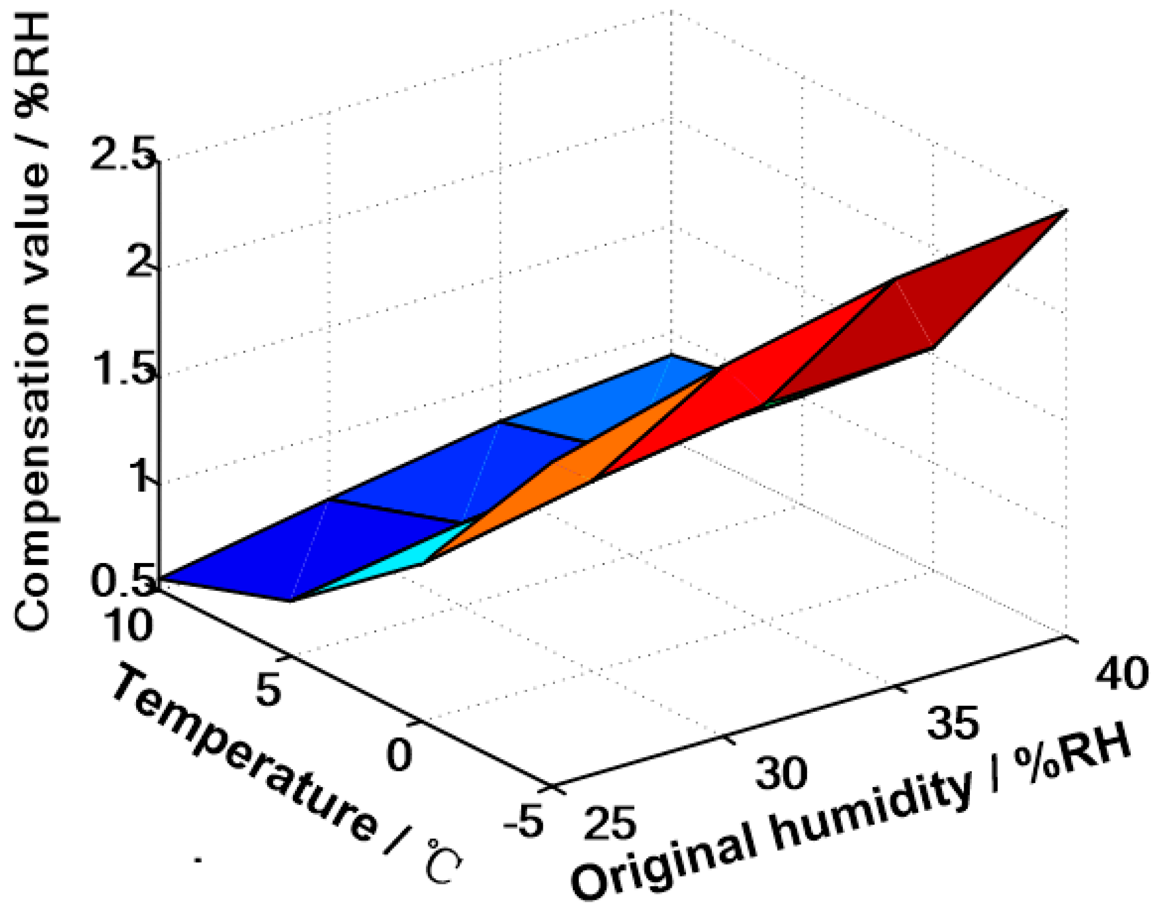
From the error curve of Figure 2, it can be seen that the error of the humidity sensor obviously increases in low and high temperature regions and has nonlinear characteristics. The original measurement value of the sensor was compensated according to different ambient temperatures, such that the compensated value was close to the standard value. Setting the ambient temperature , the relationship between the original measured value of the humidity sensor and the compensated humidity value is Equation (1).
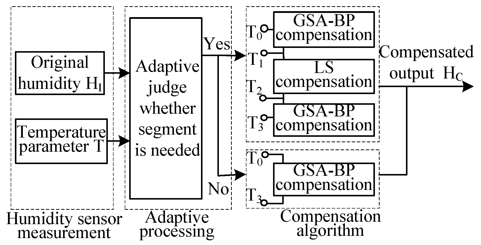
and are both single-valued functions of , then the inverse function exists. So the introduced influence parameter and the measured value were used as data to be compensated, and the regression analysis was performed by the binary linear regression function. The regression effect and the value of the segmentation point , were determined based on the value of the coefficient of determination . The least squares method and GSA-BP neural network were used to compensate the different temperature intervals. The function of segmentation compensation is similar to Equation (2).
Among these values, , is the compensation function of the temperature range with good linear regression effect. A simple and efficient least squares method was used for line fitting. and are compensated functions at low temperature and high temperature, respectively, and the GSA-BP neural network was used. The influence of temperature T was effectively reduced, and the measured data were approximated to the stand value of humidity. The overall idea of optimal compensation is shown in Figure 3.
3. Adaptive Segmentation Based on Multiple Linear Regression
For the humidity measurement errors at different temperatures, the key to improve the accuracy of compensation is to judge whether the segmentation compensation is necessary and find the best segmentation point. The linear regression method mainly determines how to obtain the best fitting line through the sample. The process is a mathematical optimization method, and it searches for the best function of data by minimizing the square of error [14]. In the regression analysis, two or more independent variables were included, and these independent variables can be approximated by a straight line. As seen from Figure 2, in the temperature experiment of the humidity sensor, there is a certain linear relationship between the measured error of humidity sensor and the temperature value in some intervals. The multivariate linear regression method can be used to analyze and compensate errors in linear intervals [15]. The regression model between the expected ideal humidity value, the measured value and the temperature was established. The coefficient of determination was calculated and whether it needed segmentation compensation according to its value was determined.
A multiple linear regression model for temperature compensation was established, such as Equation (3).
where is the expected humidity value of the regression, is the measured value of the humidity sensor, is the value of the ambient temperature, represents the i-th group data, , there are sets of data, and , , are the regression coefficients. The actual regression model can be expressed as Equation (4).
where , and are the estimated values of , and , respectively. is the estimated value of , and the residual of them is . It can be known from the least squares method that , and should minimize the sum of squares of the residuals .
According to the extremum principle of multivariate function, when gets the minimum value, the partial derivatives of to , and are all equal to zero. Then there is Equation (6).
Then Equation (7) is derived.
Its matrix form is
In Equation (8), two of the matrices can be written as
Assume
Then, Equations (9) and (10) can be rewritten as
Substitute Equation (12) and Equation (13) into Equation (8)
Thus, the regression coefficients are obtained by Equation (15)
By taking the regression coefficients into the multiple linear regression model, a compensation function can be obtained. To verify the rationality of the model, the coefficient of determination is used to estimate the fit of the model to the measured data. In multiple regression analysis, the coefficient of determination is the square of the path coefficient, that is
In Equation (16), is the average expected humidity value of . The total dispersion square sum reflects the discrete state of all expected humidity values . The regression square sum reflects the difference after regression. The sum of squared residuals is , so . Then, Equation (16) can be rewritten to Equation (17)
The coefficient of determination represents the interpretation degree of the estimated value to the ideal value . The larger the , the closer the regression curve is to the ideal humidity value [16].
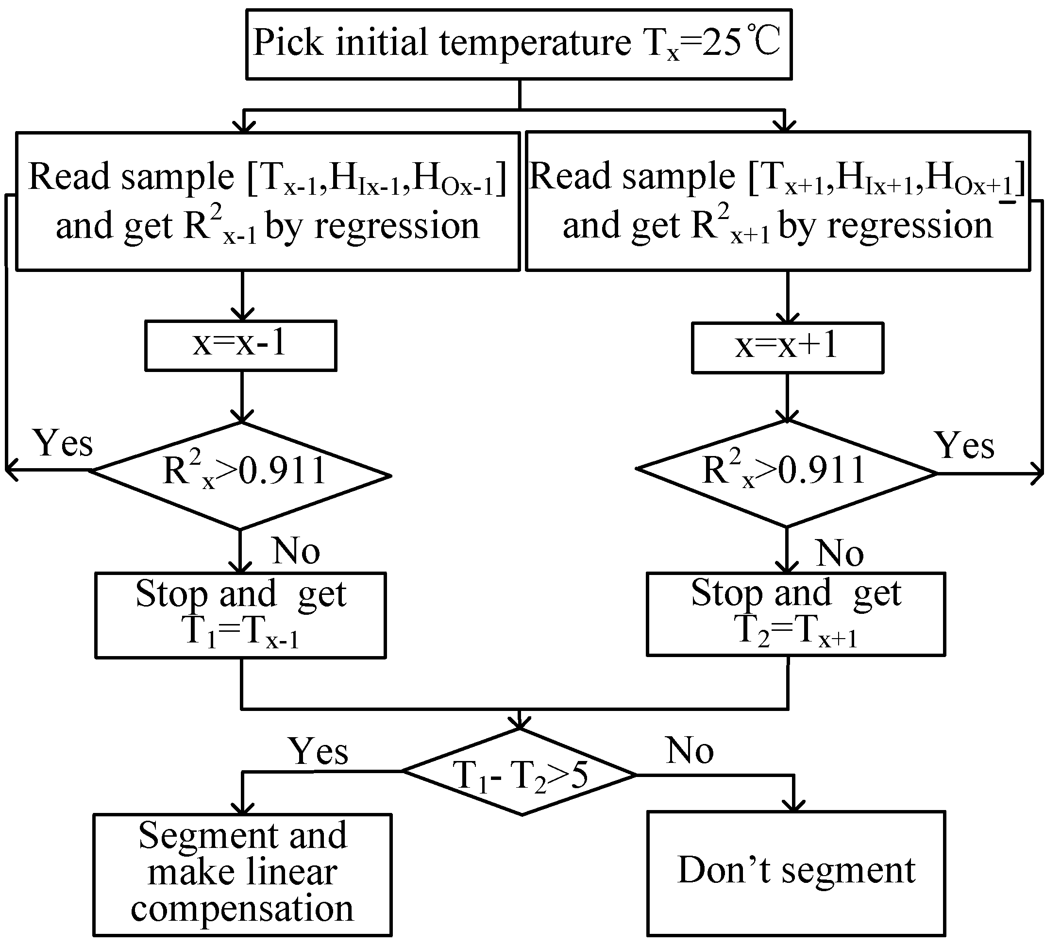
Therefore, the regression coefficients , , and coefficient of determination are calculated by using the actual measured humidity value , temperature value and the expected ideal humidity value .The coefficient of determination is used to judge whether to segment and to determine the segmentation point. The specific implementation steps are as follows.
- The error curve of humidity sensor is linear at room temperature. So the initial temperature value is determined to be about 25 °C. The measured error of humidity sensor at the ambient temperature 25 °C is −6%–−1% when the humidity is 10%–90% RH.
- Read the previous temperature value and the next temperature value and their respective humidity values.
- Each time a set of temperature and corresponding humidity data are read, a regression is performed to obtain a coefficient of determination .
- If , return to step 2, if , get the segmentation points and .
- When the temperature interval of the linear interval is greater than 5 °C, that is, , the segmentation compensation will be performed according to Figure 3. If , the whole process will be compensated by GSA-BP. An adaptive segmentation flowchart based on multiple linear regression is shown in Figure 4.
The multiple linear regression method is used to analyze the humidity measurement errors at different temperatures. For the intervals with better linearity, the multiple regression model established by Equation (4) is used to compensate the errors.
4. Nonlinear Compensation Model
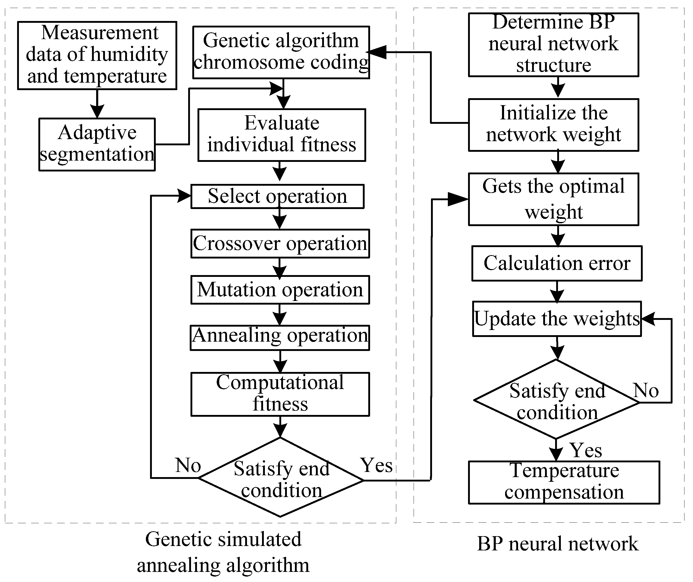
The nonlinear interval adopts the BP neural network with strong nonlinear mapping ability to compensate. The input of the BP neural network is temperature and the measured value , and the output is the compensated humidity value . The humidity sensor temperature compensation model was established, and the BP neural network was trained by multiple sets of data. To improve the local minimum of the BP neural network, a genetic simulated annealing algorithm was used.
The genetic simulated annealing algorithm is an optimization algorithm that combines a genetic algorithm and a simulated annealing algorithm. The local search ability of the genetic algorithm is limited, but the ability to grasp the overall search process is strong. The simulated annealing algorithm has strong local search ability and can prevent the search process from falling into the local optimal solution. However, little is known regarding the state of the entire search space. It is inconvenient to make the search process enter the optimal search area, which makes the simulated annealing algorithm less efficient. However, if the genetic algorithm is combined with the simulated annealing algorithm, a global search algorithm with excellent performance can be developed [17,18].
The BP neural network based on the genetic simulated annealing algorithm (GSA-BP) is mainly divided into the determination of BP network structure and the selection of weight and threshold. The specific compensation steps are the following:
- Determine the topology structure of the BP neural network. The BP neural network is set to a three-layer network structure. The original measured value of temperature and humidity sensor are the network inputs, and the number of input nodes is 2. The number of hidden layer nodes is set to 7 according to the compensation effect. The output of the network is the humidity value after compensation, and the number of output nodes is 1. The number of optimized parameters of the genetic simulated annealing algorithm is determined as follows: .
- Initialize the genetic simulated annealing algorithm. The population size with weights and thresholds is 60; the maximum number of iterations MAXGEN is 2000; the crossover probability is 0.6; the mutation probability is 0.1; the initial temperature is 100; the end temperature is 0.99; the temperature cooling coefficient is 0.99.
- Initialize the weights and thresholds of the BP neural network and calculate fitness. The initial population of the genetic simulated annealing algorithm is generated by combining the initial weights and thresholds of the BP neural network initialization with the original measured values and temperature . Each individual in the genetic simulated annealing algorithm represents all the weights and threshold of a network, and the algorithm then calculates the fitness of each individual through a fitness function. The fitness function of this paper adopts the fitness stretching method, and the fitness of the i-th individual after improvement is calculated by Equation (18).Among these values, is the i-th individual fitness before improvement, . and are the initial temperature and the current temperature in the simulated annealing algorithm respectively, . is the current genetic evolution algebra, and is the population size. and are the standard humidity values expected and the humidity values actually obtained by the network of the i-th individual.
- The genetic simulated annealing algorithm finds individuals with optimal fitness based on a series of operations such as selection, crossover, mutation and annealing. Compare the current fitness and historical best fitness of each individual in the population. If the current value is better, the current value is the best value of the history, and save the individual as the best value of history, otherwise the best value will not change.
- The genetic simulated annealing algorithm obtains the optimal individual as the initial weight and threshold of the BP neural network. The optimized BP neural network is used to train the humidity data at different temperatures.
Figure 5 shows the process of the compensation method of the humidity sensor. After inputting the original measured values of the humidity sensors and ambient temperature, the GSA optimizes the weights and thresholds of the BP neural network. Finally, the compensated humidity value is obtained.
5. Experimental Results and Analysis
5.1. Performance Analysis of Optimized Compensation Algorithm GSA-BP
The variables of the segmentation compensation function are the actual measured value of the humidity sensor and the ambient temperature value. GSA is a random search algorithm. The number of iterations is uncertain. The representative training process was compared with the BP neural network, which is not optimized.
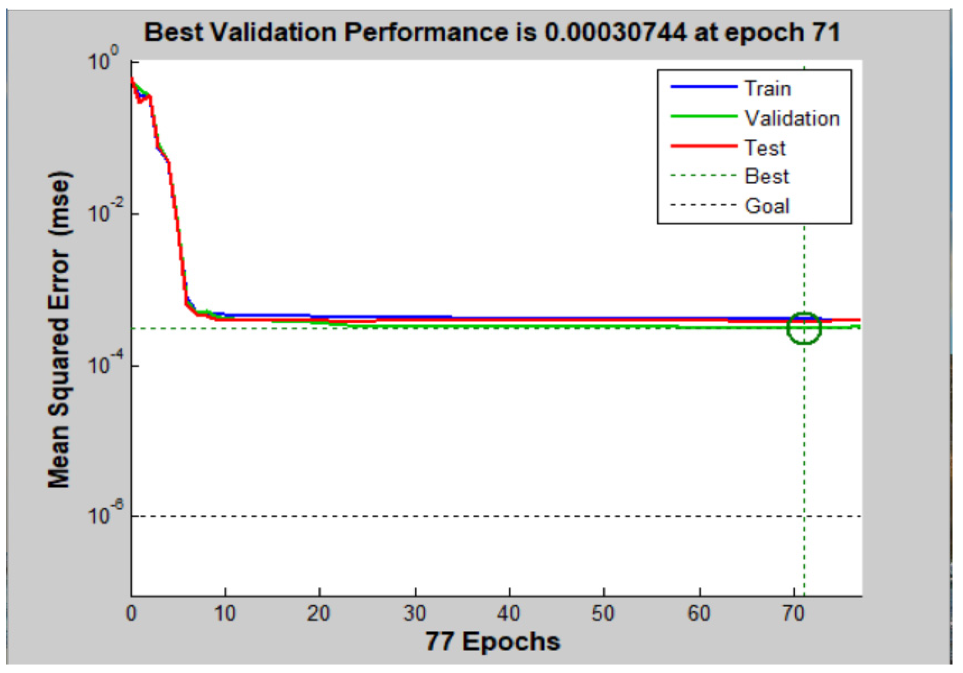
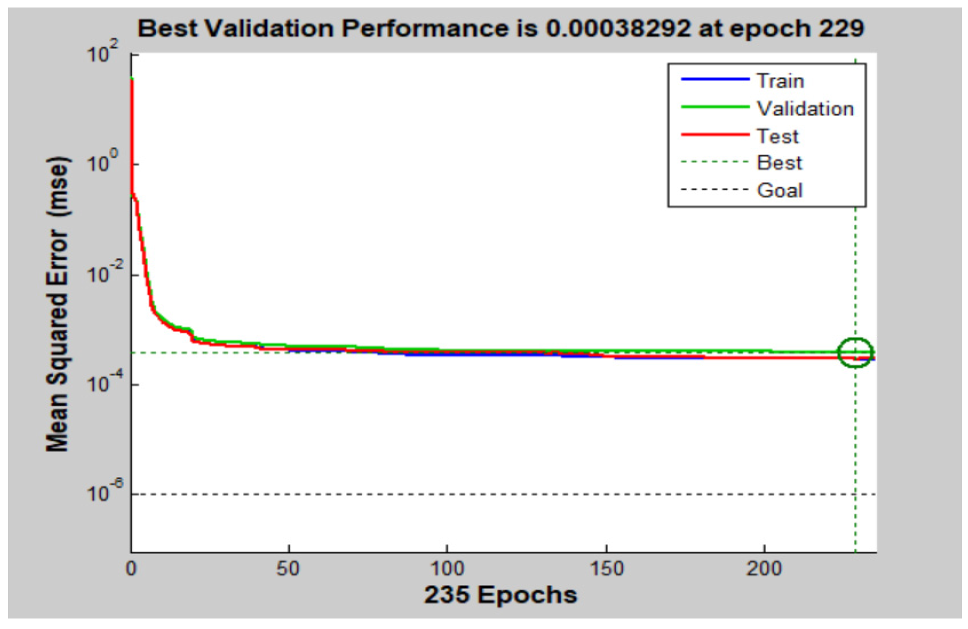
It can be seen from Figure 6 that when the GSA-BP neural network evolves to 70 generations, its adaptation value reaches a minimum, the optimal weight and threshold of the BP neural network are found, and the number of termination iterations is 77. In Figure 7, the number of iterations of the BP neural network is 229. It can be seen that under the same conditions, the number of iterations of the BP neural network optimized by GSA is small, and the training speed is fast, which indicates that the BP neural network optimizes the operation efficiency significantly.
Figure 8 is the humidity compensation effect curve of the GSA-BP neural network. It can be seen from the figure that the errors between the predicted output and the expected output are very small, and the BP neural network optimized by GSA has a good compensation effect.
5.2. Segmentation Optimization Compensation Model
Through the above theoretical analysis and verification of experimental data, the influence of temperature on the humidity sensor can be seen. One hundred and fifty sets of data obtained by repeating experiments on the same humidity sensor were used as training samples, and 15 sets of data were used as network test samples. The process of establishing a humidity compensation model is as follows:
- Read the measured data set and interpolate it. The temperature points set in the experiment have some discreteness. So the continuous function is added on the basis of the discrete data and that the continuous curve passes all the given discrete data points. The interpolated data will be compensated for later.
- Read two groups of temperature and corresponding humidity in sequence from the temperature of 25 °C, use the binary linear regression function to regress the data after interpolation, and determine the regression effect according to the value of the criterion . When , the regression is stopped. The value of is 0.8468 when the experimental data stops returning. The temperature value at this time is the temperature segmentation points , , which are 22.36 and 29.98, respectively.
- Determine whether the interval of the temperature segmentation point is greater than 5. The experimental data satisfy this condition; therefore, segmentation compensation is made. The least squares method is used for linear fitting of the temperature range . Taking the straight line fitting effect of 30% RH as an example, the fitted straight line is: , where is the compensation value, and is the temperature value. When the value of measured humidity is 30% RH, input the value of temperature and obtain the corresponding humidity compensation value, then add the measured value to obtain the compensated value.
- Use GSA to optimize the weight and threshold of the BP neural network, train the neural network, and compensate the data in the nonlinear interval.
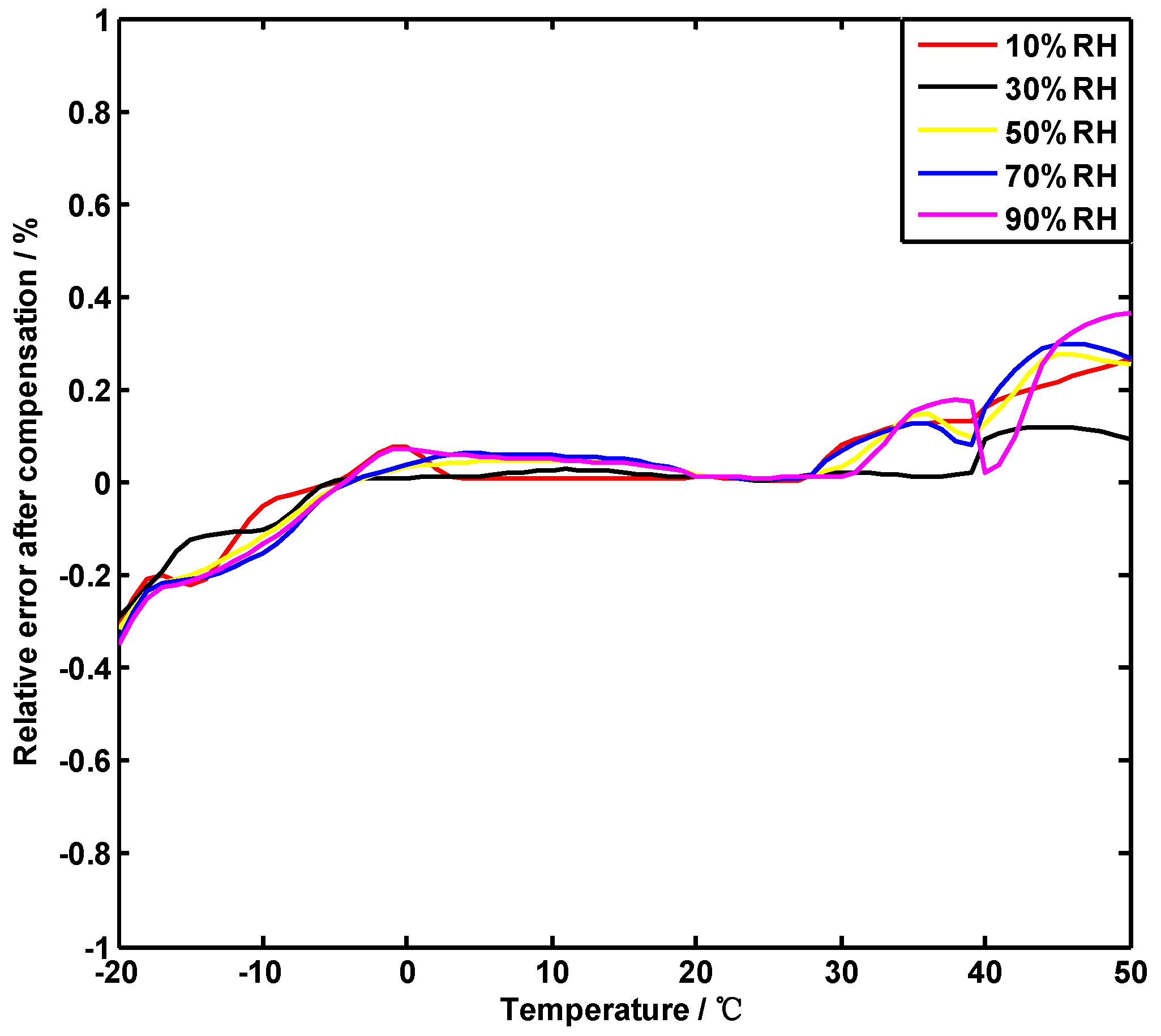
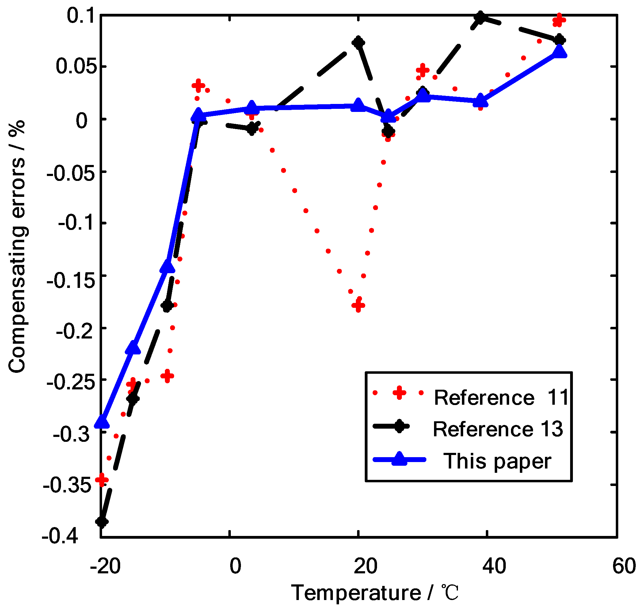
The original measurement data of the same humidity sensor were compensated by using reference 11, reference 13 and the method proposed in this paper. Reference 11 used a genetic algorithm (GA) improved BP neural network without segmentation compensation, where GA is a population-based optimization algorithm [19]. Reference 13 used a least squares and BP neural network to compensate. In this paper, the BP neural network improved by adaptive selection and combined with genetic simulated annealing was used for compensation. To avoid the randomness of the algorithm, the same group of data was run many times, and the compensation effect was the same; therefore, the average value of the same group of data after multiple runs was taken. The three methods compensate the data as shown in Table 1, and the corresponding error curve is shown in Figure 11.
- The overall trend of the compensation effects of the three methods is the same. The compensation error used in reference 11 is large, and the error at the segmentation node significantly increased. The compensation effect of the method in this paper is relatively stable. In particular, the curve between 0 and 40 °C tends to be gentle and close to zero.
- The adaptive segmentation compensation method combines the simplicity and efficiency of the least squares method with the high precision of the GSA-BP neural network. The measurement error of humidity significantly improved over the entire temperature range. In the vicinity of the segmentation point (22.36 °C, 29.98 °C) obtained by the adaptive calculation, the compensation effect is particularly significant.
6. Conclusions
We use this method to compensate for humidity sensors of different temperature ranges and different individual temperatures. According to the error curve under different ambient temperatures, multiple linear regression analysis was used to determine the segmentation points, and different algorithms were used to compensate. The results show that the method has strong universality and is effective for different temperature ranges and individual measurements.
In addition, the introduction of independent component analysis method into the reconstruction of measured error might further improve the compensation effect [20]. It should be added that the initial temperature is 25 °C when determining the segmentation point in this method. This temperature is employed because the humidity error of the sensor used in this experiment is relatively linear at approximately 25 °C after multiple measurements. If other sensors are used, the initial values will be determined according to the humidity curves of those different sensors. However, the initial values will be not very strict, and the nearby values can be adaptively processed as initial values.
Author Contributions
Conceptualization, W.X. and X.F.; Methodology, W.X.; Software, X.F.; Validation, X.F. and W.X.; Data Curation, H.X.; Writing-Original Draft Preparation, X.F. and W.X.; Writing-Review & Editing, W.X.; Supervision, W.X.; Project Administration, H.X.; Funding Acquisition, W.X.
Funding
This work is supported by the National Key R&D Program of China (2018YFC1506102) and the National Natural Science Foundation of China (Grant NO. 41605121 and NO. 61671248).
Conflicts of Interest
The authors declare no conflicts of interest.
References
- Weiwei, L.V.; Xiaohua, L.V.; Zuoyang, T.; Xiaohua, X.; Yong, X. Fault Analysis and Maintenance of DZZ Series of Automatic Weather Stations. Meteorol. Environ. Res. 2018, 9, 35–37. [Google Scholar]
- Hai, M.; Wen, F.; Wang, C.; Li, X.J. Capacitive humidity sensing properties of CdS/ZnO sesame-seed-candy structure grown on silicon nanoporous pillar array. J. Alloys Compd. 2017, 11, 94–98. [Google Scholar]
- Lob, V.; Geisler, T.; Brischwein, M.; Uhl, R.; Wolf, B. Humidity sensor using a single molecular transistor. J. Appl. Phys. 2015, 118, 135–171. [Google Scholar]
- Wang, D.F.; Lou, X.; Bao, A.; Yang, X.; Zhao, J. A temperature compensation methodology for piezoelectric based sensor devices. Appl. Phys. Lett. 2017, 111, 083502. [Google Scholar] [CrossRef]
- Ruirong, D.; Hongwei, Z.; Nan, S.; Bo, D.; Dengyue, W. Compensation and calibration of the high temperature and pressure downhole pressure sensor. Chin. J. Sci. Instrum. 2016, 43, 737–743. [Google Scholar]
- Hsieh, C.; Hung, C.; Li, Y. Investigation of a Pressure Sensor with Temperature Compensation Using Two Concentric Wheatstone-Bridge Circuits. Mod. Mech. Eng. 2013, 10, 104–113. [Google Scholar] [CrossRef]
- Zhou, G.; Zhao, Y.; Guo, F. A Smart High Accuracy Silicon Piezoresistive Pressure Sensor Temperature Compensation System. Sensors 2014, 4, 74–90. [Google Scholar] [CrossRef] [PubMed]
- Li, T.; Liang, S.; Hong, Y.; Pan, L. Simulation of Temperature Compensation of Pressure Sensor Based on PCA and Improved BP Neural Network. Adv. Mater. Res. 2014, 846–847, 513–516. [Google Scholar] [CrossRef]
- Li, Y.; Li, Y.; Li, F.; Zhao, B. The Research of Temperature Compensation for Thermopile Sensor Based on Improved PSO-BP Algorithm. Math. Probl. Eng. 2015, 3, 1–6. [Google Scholar] [CrossRef]
- Zhu, L.; Xie, B.; Xing, Y.; Chen, D.; Wang, J. A Resonant Pressure Sensor Capable of Temperature Compensation with Least Squares Support Vector Machine. Procedia Eng. 2016, 168, 1731–1734. [Google Scholar] [CrossRef]
- Jiwei, P.; Wenhua, L.V.; Hongyan, X.; Xiangjuan, W. Temperature compensation for humidity sensor based on improved GA-BP neural network. Chin. J. Sci. Instrum. 2013, 34, 153–160. [Google Scholar]
- Guo, M.; Xing, H.; Zhang, D.; Zhang, L. Temperature Compensation for Humidity Sensor Based on the AFSA-BP Neural Network. Instrum. Tech. Sens. 2017, 8, 6–10. [Google Scholar]
- Xing, H.Y.; Peng, J.W.; Lv, W.H. A fusion algorithm for humidity sensor temperature compensation. Chin. J. Sens. Actuators 2012, 25, 1711–1716. [Google Scholar]
- Kutner, M.; Nachtsheim, C.; Neter, J. Applied Linear Regression Models; McGraw-Hill/Irwin Education: New York, NY, USA, 2004. [Google Scholar]
- Dos Soares, T.S.; Mendes, D.; Rodrigues, T.R. Artificial neural networks and multiple linear regression model using principal components to estimate rainfall over South America. Nonlinear Process. Geophys. 2016, 23, 1317–1337. [Google Scholar]
- Xu, W.; Li, F.; Liu, F. Optimality and Recursive Algorithm of General Least Squares Estimator of Seemingly Unrelated Linear Regression Models. In Proceedings of the 2010 International Conference on Computational Intelligence and Software Engineering, Wuhan, China, 10–12 December 2010. [Google Scholar]
- Shidrokh, G.; Hassan, W.H.; Hossein, M.; Seyed, A.; Soleymani, A. MDP-Based Network Selection Scheme by Genetic Algorithm and Simulated Annealing for Vertical-Handover in Heterogeneous Wireless Networks. Wirel. Pers. Commun. 2017, 2, 399–436. [Google Scholar]
- Örkcü, H.H. Subset selection in multiple linear regression models: A hybrid of genetic and simulated annealing algorithms. Appl. Math. Comput. 2013, 5, 11018–11028. [Google Scholar]
- Wang, K.; Luo, X.; Shen, H.; Zhang, H. GSA-BP neural network model for back analysis of surrounding rock mechanical parameters and its application. Rock Soil Mech. 2016, 37, 631–638. [Google Scholar]
- Chen, X.; Ma, D. Mode Separation for Multimodal Ultrasonic Lamb Waves Using Dispersion Compensation and Independent Component Analysis of Forth-Order Cumulant. Appl. Sci. 2019, 9, 555. [Google Scholar] [CrossRef]
Figure 1.
Error experiment of humidity sensor at different temperatures.

Figure 2.
Measured error curve of the humidity sensor at different temperatures.

Figure 3.
Compensation principle of humidity sensor.

Figure 4.
Flow chart of searching segmentation point.

Figure 5.
Flow chart of compensation algorithm based on genetic simulated annealing (GSA-BP).

Figure 6.
Training iterations of GSA-BP neural network.

Figure 7.
Training iterations of back propagation (BP) neural network.

Figure 8.
Compensation curve of GSA-BP neural network.

Figure 9.
Compensation function model.

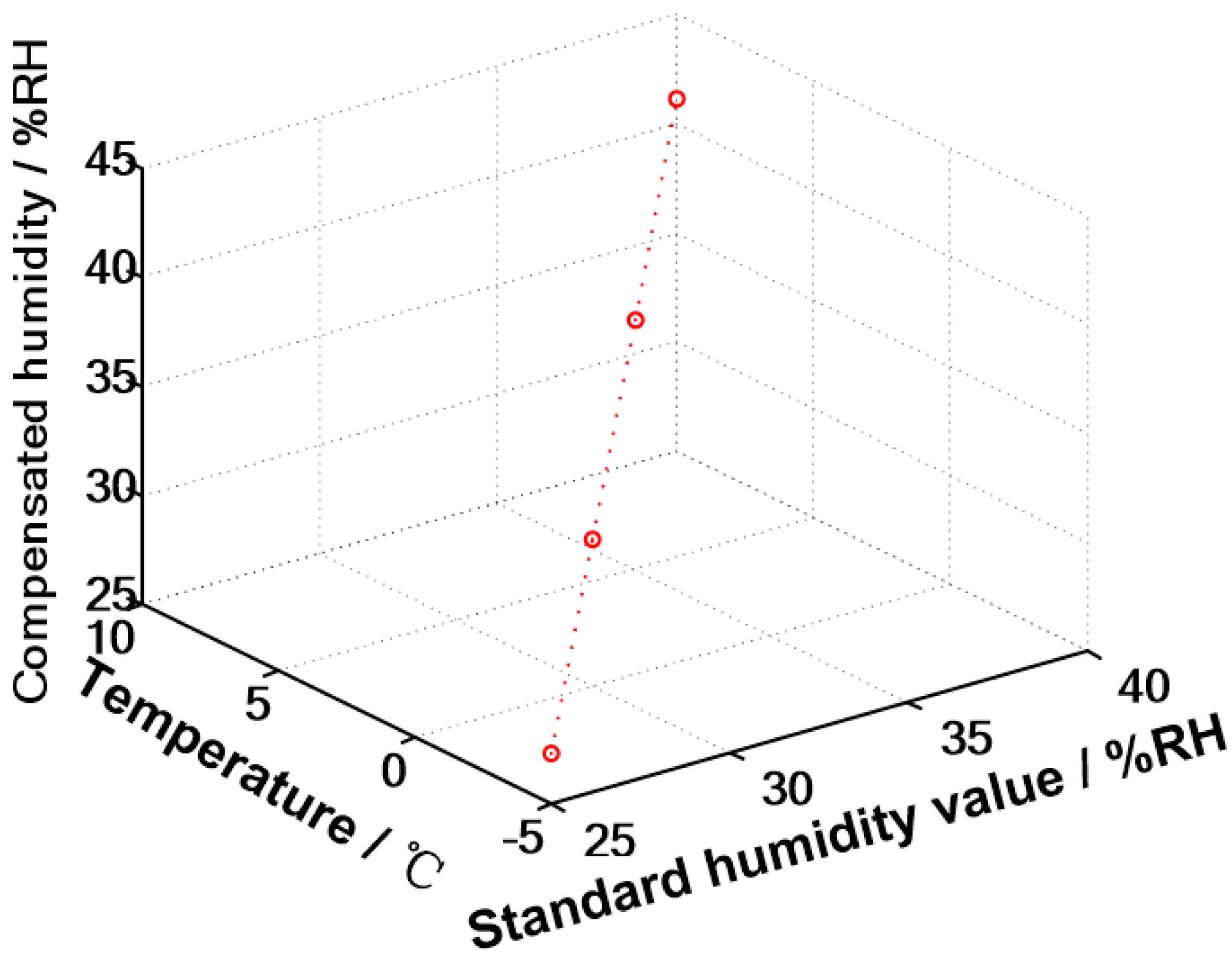
Figure 10.
Compensation effect.

Figure 11.
Error curve after compensation by three methods.


Table 1.
Error after compensation of three methods.
| Environment Temperature (°C) | Standard Value of Relative Humidity (%RH) | Error of Different Methods of Compensation (%) | ||
|---|---|---|---|---|
| Reference 11 | Reference 13 | This Paper | ||
| −19.68 | 11.79 | −0.34553 | −0.3857 | −0.2912 |
| −14.98 | 11.56 | −0.25367 | −0.2678 | −0.2198 |
| −9.65 | 11.15 | −0.24591 | −0.1783 | −0.1423 |
| −4.78 | 9.26 | 0.0321 | −0.0026 | 0.0035 |
| 3.45 | 9.61 | 0.0056 | −0.0098 | 0.0102 |
| 20.01 | 23.55 | −0.1785 | 0.0728 | 0.0128 |
| 24.58 | 25.05 | −0.0148 | −0.0118 | 0.0021 |
| 29.98 | 25.95 | 0.04726 | 0.0248 | 0.0219 |
| 38.89 | 27.8 | 0.0147 | 0.0975 | 0.0175 |
| 51.21 | 29.25 | 0.0947 | 0.0752 | 0.0642 |
© 2019 by the authors. Licensee MDPI, Basel, Switzerland. This article is an open access article distributed under the terms and conditions of the Creative Commons Attribution (CC BY) license (http://creativecommons.org/licenses/by/4.0/).
Share and Cite
MDPI and ACS Style
Xu, W.; Feng, X.; Xing, H. Modeling and Analysis of Adaptive Temperature Compensation for Humidity Sensors. Electronics 2019, 8, 425. https://doi.org/10.3390/electronics8040425
AMA Style
Xu W, Feng X, Xing H. Modeling and Analysis of Adaptive Temperature Compensation for Humidity Sensors. Electronics. 2019; 8(4):425. https://doi.org/10.3390/electronics8040425
Chicago/Turabian StyleXu, Wei, Xiaoyu Feng, and Hongyan Xing. 2019. "Modeling and Analysis of Adaptive Temperature Compensation for Humidity Sensors" Electronics 8, no. 4: 425. https://doi.org/10.3390/electronics8040425
Note that from the first issue of 2016, this journal uses article numbers instead of page numbers. See further details here.