A Modified Model Predictive Power Control for Grid-Connected T-Type Inverter with Reduced Computational Complexity

Abstract

This study proposed a modified power strategy based on model predictive control for a grid-connected three-level T-type inverter. The controller utilizes the mathematical model to forecast the performance of the grid current, the balance of DC-bus capacitor voltages and switching frequency. The proposed method outlines a new technique to formulate a control objective. The control objective includes the absolute error of the inverter voltage reference and its possible values instead of the grid current error. By using the modified equivalent transformations in the cost function, the execution time was reduced 22% compared to the traditional model predictive control while maintaining the high dynamic performances of the power and low total harmonic distortion of the current. A comparative investigation showed that the proposed method obtains a high-performance control compared with the classical power control scheme with linear PI controllers and space vector modulation. The feasibility of the proposed method was verified by the simulation and experimental results.

1. Introduction

Over the last few years, multilevel converters have been recognized as an alternative approach for high-power electronics owing to the improvement of capacity and performance compared with the two-level converter [1,2,3]. In particular, the T-type inverter topology is preferred due to the benefits in term of low conduction losses and high sinusoidal waveforms of the output voltage [4,5]. The unbalance of capacitor voltages is the big problem for this configuration. However, this issue has been addressed by several methods [6,7,8,9,10].

Grid-connected power converters have proven to be important in many industrial applications such as active power filters, distributed systems, and renewable power generation systems [11,12,13,14,15,16]. The conventional control strategy is the voltage-oriented control [11,13] which can ensure the steady-state and performance via the traditional PI current controllers with pulse width modulation (PWM) or space vector modulation (SVM). However, the completeness of the current decoupling of the internal current controller and accurate tuning parameters are the drawbacks of this method. This technique has a low dynamic response and is not suitable for a nonlinear system. Recently, to improve the performance, direct power control (DPC) [17] has been presented by employing a look-up table to decide the proper switching state of the inverter. Nonetheless, a big ripple of the active and reactive powers is the problem of this approach. Moreover, it is necessary to require a small sampling time to obtain a reasonable steady-state and good transient performances. To overcome these issues, various approaches have been developed such as using DPC established on extended-state observation with PWM [18], port-controlled Hamiltonian system [12], sliding mode control [19], and predictive control [20,21,22,23].

Over the last decade, many researchers have focused on a finite control set model predictive control (FCS-MPC) for power electronics applications due to its simplicity of configuration, easy realization, and rapid transient response [24,25,26,27]. Besides, the benefits of FCS-MPC are that the non-linearities, delay compensation and additional constraints are easily imposed on the controller. However, in the FCS-MPC, every state needs to be enumerated to achieve the optimal value, leading to the computational burden becoming a major issue, especially with a high number of switching states such as multilevel inverters and long prediction horizons. To deal with this problem, a simplified MPC is put forward in [28] for converters. This method employs switching state group for optimization loop to reduce the computation time. An alternative technique mentioned for multilevel converters [29,30] is to reduce the computational cost by developing a modified sphere decoding algorithm. In [31], the equivalent transformation in the cost function is employed in the optimization loop to reduce the time-consuming computation for converters with inductive load load. The modified algorithm in [32] incorporates the conventional FCS-MPC and steady-state assessment to decrease the computational cost. Nonetheless, the computational burden of this approach is large, similar to the conventional FCS-MPC in the unfavorable case. The proposed approach is presented in [22] to reduce the execution time by using the preselected voltage reference and DC-bus capacitor voltage balancing. Nonetheless, this method is only applied to a 3L-T-type inverter with LC filter in standalone mode.

We here refine the method in [31] by taking into account the computational delay in the control design for grid-connected to the 3L-T-type inverter. This approach not only keeps the DC-link capacitor voltage balancing and decreases the switching frequency but also guarantees the high-performance control. The cost function based on the model predictive control is utilized to achieve these purposes. A control horizon of modified one-step prediction is used to compensate the computational delay, diminish the power ripples and enhance the control performance. Compared with linear controllers, the proposed method has a fast dynamic response and no overshoot of transient response. Furthermore, to address the aforementioned challenge, this research aimed to develop the cost function for reducing the computational effort in the optimization problem. The formula of the cost function consists of the current tracking error with the conventional model predictive current control method. In this research, a predictive model of grid current was employed to obtain the required inverter voltage. Then, the revised cost function, which includes the inverter output voltage errors, neutral-point voltage and switching frequency reduction, was defined. Consequently, the computational burden of the proposed method was reduced by 22% compared to the traditional FCS-MPC, providing the practicality of the real-time implementation. Simulation and experiments were used to evaluate and verify the performance of the proposed method.

This paper is structured as follows: Section 2 introduces the dynamic model of a predictive control strategy based on voltage orientation for a grid-connected 3L-T-type inverter. Section 3 outlines the proposed modified model predictive control strategy to reduce the computational cost. In Section 4, a performance comparison between the proposed method and traditional FCS-MPC and the classical DPC with linear PI controllers and SVM (DPC-SVM) is presented. Section 5 summarizes some conclusions.

2. Dynamic Modeling for Grid-Connected 3L-T-Type Inverter

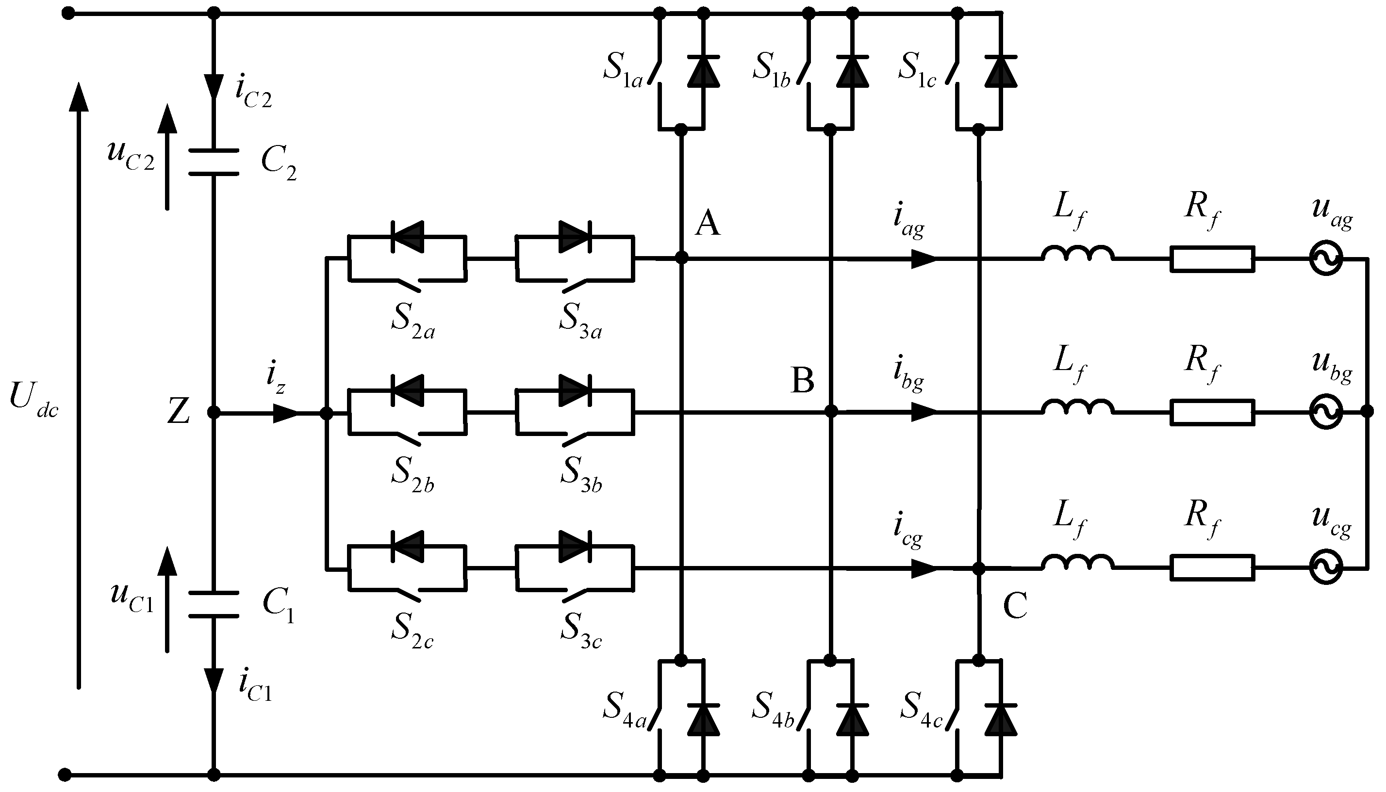
2.1. Configuration of the Grid-Connected 3L-T-Type Inverter

A simplified circuit of the grid connected 3L-T-type inverter is illustrated in Figure 1. The operating principle of each inverter branch can be described by three switching statuses [1], [0], and [−1]. During switching status [1] or [P], both switches $S_{1x}$ and $S_{2x}$ with $x\in \left\{a,b,c\right\}$ are turned “ON” leading to $u_{xZ}=U_{dc}/2$, while [−1] or [N] signifies two switches $S_{1x}$ and $S_{2x}$ are turned “OFF”, resulting $u_{xZ}=-U_{dc}/2$. The switching state [0] or [O] means that the two internal switches $S_{2x}$ and $S_{3x}$ are “ON” and $u_{xZ}$ is clamped to zero. Thus, taking into account the three phases of the inverter, 27 possible configurations are produced for the 3L-T-type. The summary of switching states generated by this inverter is presented in

Table 1. Operating principle of inverter branch x.

Switching State	Switches				One Phase Inverter Voltage
${\mathit{S}}_{\mathit{x}}$	${\mathit{S}}_{\mathbf{1}\mathit{x}}$	${\mathit{S}}_{\mathbf{2}\mathit{x}}$	${\mathit{S}}_{\mathbf{3}\mathit{x}}$	${\mathit{S}}_{\mathbf{4}\mathit{x}}$	${\mathit{u}}_{\mathit{xZ}}$
N	0	0	1	1	$-U_{dc}/2$
O	0	1	1	0	0
P	1	1	0	0	$U_{dc}/2$

.

2.2. Mathematical Model

The inverter output voltage generated by the 3L-T-type can be defined:

$$u_{inv}={\displaystyle \frac{2}{3}}\left(u_{AZ}+m{u}_{BZ}+m^2{u}_{CZ}\right),$$

(1)

where $u_{AZ}$, $u_{BZ}$, and $u_{CZ}$ are the three-phase inverter voltage, relating to the neutral-point Z of the DC-bus; and $m=e^{j2\pi /3}=-\frac{1}{2}+j\frac{\sqrt{3}}{2}$.

The phase to neutral voltages $u_{xZ}$ of the 3L-T-type inverter are calculated in terms of the switching status $S_x$ and DC-bus voltage $U_{dc}$ [7,27]:

$$u_{xZ}=S_x{\displaystyle \frac{U_{dc}}{2}},$$

(2)

where $S_x$ stands for the status of an inverter branch with three possible combinations $\{-1,0,1\}$.

Under the assumption of a constant DC-bus voltage and $C_1$ = $C_2$ = $C_{dc}$, the dynamic of neutral-point voltage ($u_z$) can be phrased in terms of the switching states and the grid currents [22]:

$$\begin{array}{c}{\displaystyle \frac{d{u}_z}{dt}}={\displaystyle \frac{d\left(u_{c1}-u_{c2}\right)}{dt}}=-{\displaystyle \frac{1}{C_{dc}}}{i}_z=-{\displaystyle \frac{1}{C_{dc}}}\left((1-|S_a|)i_{ag}+(1-|S_b|)i_{bg}+(1-|S_c|)i_{cg}\right).\hfill \end{array}$$

(3)

The mathematical model of grid-connected inverter is given by:

$$u_{inv}=u_g+R_f{i}_g+L_f\frac{d{i}_g}{dt},$$

(4)

where $u_g={\left[u_{ag},u_{bg},u_{cg}\right]}^T$, $i_g={\left[i_{ag},i_{bg},i_{cg}\right]}^T$ are the grid voltage and current vectors and $R_f$, $L_f$ are the filter resistance and inductance, respectively.

The dynamics model in the $dq$ synchronous reference frame is derived from the rotational transformation of Equation (4) as follows:

$$\begin{array}{cc}{u}_{inv\_d}& =R_f{i}_d+L_f{\displaystyle \frac{d{i}_d}{dt}}+u_d-\omega L_f{i}_q,\\ u_{inv\_q}& =R_f{i}_q+L_f{\displaystyle \frac{d{i}_q}{dt}}+u_q+\omega L_f{i}_d,\end{array}$$

(5)

where $\omega$ is the grid frequency.

Considering the grid-voltage oriented condition (Figure 2), the components of grid voltage can be achieved by:

$$u_d={\widehat{U}}_g,u_q=0,$$

(6)

where ${\widehat{U}}_g$ denotes the grid voltage magnitude that is achieved by using the phase-locked loop (PLL).

As a result, the dynamics model in continuous time is rewritten from Equations (3), (5) and (6) as:

$$\begin{array}{cc}{\displaystyle \frac{d{i}_d}{dt}}\hfill & =-{\displaystyle \frac{R_f}{L_f}}{i}_d+{\displaystyle \frac{1}{L_f}}(u_{inv\_d}-{\widehat{U}}_g)+\omega i_q,\hfill \\ {\displaystyle \frac{d{i}_q}{dt}}\hfill & =-{\displaystyle \frac{R_f}{L_f}}{i}_q+{\displaystyle \frac{1}{L_f}}{u}_{inv\_q}-\omega i_d,\hfill \\ \frac{d{u}_z}{dt}\hfill & =\frac{1}{2C_{dc}}(2|S_a|-|S_b|-|S_c|)i_{\alpha }+\frac{\sqrt{3}}{2C_{dc}}(|S_b|)-|S_c|)i_{\beta },\hfill \end{array}$$

(7)

where the grid current components in the $dq$ coordinate frame are achieved by their values in the $\alpha \beta$ stationary reference frame by using Park transformation:

$$\begin{array}{cc}{i}_d\hfill & =i_{\alpha }cos\theta +i_{\beta }sin\theta ,\hfill \\ i_q\hfill & =i_{\beta }cos\theta -i_{\alpha }sin\theta .\hfill \end{array}$$

(8)

Similarly, the component of inverter voltage is expressed based on Equations (1) and (2) as:

$$\begin{array}{cc}{u}_{inv\_d}\hfill & =u_{inv\alpha }cos\theta +u_{inv\beta }sin\theta ,\hfill \\ u_{inv\_q}\hfill & =u_{inv\beta }cos\theta -u_{inv\alpha }sin\theta ,\hfill \end{array}$$

(9)

where $u_{inv\alpha }$ and $u_{inv\beta }$ are the elements of inverter voltage which are achieved from the Clarke transformation:

$$\begin{array}{cc}{u}_{inv\alpha }\hfill & ={\displaystyle \frac{U_{dc}}{6}}\left(2S_a-S_b-S_c\right),\hfill \\ u_{inv\beta }\hfill & ={\displaystyle \frac{\sqrt{3}{U}_{dc}}{6}}\left(S_b-S_c\right).\hfill \end{array}$$

(10)

We can calculate the grid active and reactive powers as [11,17]:

$$\begin{array}{cc}{P}_g\hfill & ={\displaystyle \frac{3}{2}}\left(u_d{i}_d+u_q{i}_q\right)={\displaystyle \frac{3}{2}}{\widehat{U}}_g{i}_d,\hfill \\ Q_g\hfill & ={\displaystyle \frac{3}{2}}\left(u_q{i}_g-u_d{i}_q\right)=-{\displaystyle \frac{3}{2}}{\widehat{U}}_g{i}_q.\hfill \end{array}$$

(11)

Equation (11) means that we can employ the grid current components to control the active and reactive powers.

3. Proposed Control Strategy Based on Model Predictive Control

The purposes of the proposed method are to:

• Follow the active and reactive power references.
• Ensure the capacitor voltage balancing.
• Decrease the frequency of the switches.

With the aim to accomplish the control goal, the cost function of the conventional FCS-MPC for the grid system, which takes into account the one-step prediction and delay compensation, is presented as [25,26]:

$$\begin{array}{cc}\hfill g_{cnv}& =\left|i_d^{*}(k+2)-i_d^p(k+2)\right|+\left|i_q^{*}(k+2)-i_q^p(k+2)\right|+{\lambda }_{dc}\left|u_z^p(k+2)\right|+{\lambda }_{n}s{w}_c,\hfill \end{array}$$

(12)

where $i_d^{*}(k+2)$, $i_q^{*}(k+2)$ and $i_d^p(k+2)$, $i_q^p(k+2)$ represent the reference and predicted currents at instant $k+2$, respectively. ${\lambda }_{dc}$ and ${\lambda }_n$ denote the weighting elements of the balance of capacitor voltages and switching frequency reduction.

The weighting factors ${\lambda }_{dc}$ and ${\lambda }_n$ are considered as tuning parameters to achieve an acceptable control performance. Adjusting these values is not an easy mission for the classical PI controllers. Section 4 illustrates the details of the selection of these parameters.

$s{w}_c$ in Equation (12) is the additional constraint imposed on the cost function to reduce the switching frequency of the inverter. Thus, its expression can be given by:

$$\begin{array}{c}\hfill s{w}_c=\sum _{x=a,b,c}\left|S_x(k+1)-S_x(k)\right|.\end{array}$$

(13)

In a real-time control system, it is necessary to consider a time delay produced by computation time. To overcome this problem, in the traditional approach [25,27], the predicted variables at instant $k+1$ are estimated by using the dynamic model, measurement feedback and previous switching status at instant k. Next, the associated predicted variables at time $k+2$ are obtained from the estimated variables at time $k+1$ and all switching states of the inverter. Thus, the optimal control input is achieved from cost function optimization at time $k+2$ and implemented to the inverter at $k+1$, as shown in Figure 3.

As mentioned in Section 2.2, a control action $u={\left[S_a,S_b,S_c\right]}^T$ is a finite set of feasible control associated with the switching states $u\in \mathbb{U}=\left\{u_1,u_2,\dots ,u_{27}\right\}$. Consequently, the optimal control action $u_{opt}$ is implemented in the converter at time $k+1$ by minimizing Equation (14):

$$\begin{array}{ccc}{\widehat{i}}_d(k+1)\hfill & =\hfill & f_1(i_d(k),i_q(k),u_k),{\widehat{i}}_q(k+1)=f_2(i_q(k),i_d(k),u_k),\hfill \\ i_d^p(k+2)\hfill & =\hfill & f_1({\widehat{i}}_d(k+1),{\widehat{i}}_q(k+1),u_{k+1}),i_q^p(k+2)=f_2({\widehat{i}}_d(k+1),{\widehat{i}}_q(k+1),u_{k+1}),\hfill \\ {\widehat{u}}_z(k+1)\hfill & =\hfill & f_3(i_g(k),u_z(k),u_k),u_z^p(k+2)=f_3({\widehat{i}}_g(k+1),{\widehat{u}}_z(k+1),u_{k+1}),\hfill \\ g_{cnv}(u_{k+1})\hfill & =\hfill & |i_d^{*}(k+2)-i_d^p(k+2)|+|i_q^{*}(k+2)-i_q^p(k+2)|+{\lambda }_{dc}|u_z^p(k+2)|+{\lambda }_{n}s{w}_c,\hfill \\ u_{opt}\hfill & =\hfill & arg\{\underset{u_{k+1}\in \{-1,0,1{\}}^3}{\min }{g}_{cnv}(u_{k+1})\}.\hfill \end{array}$$

(14)

Considering a sampling interval $T_s$, the discrete-time of the grid current is obtained by employing the first-order forward Euler approximation for Equation (7):

$$\begin{array}{cc}{\widehat{i}}_d(k+1)\hfill & =i_d(k)\left(1-\frac{T_s{R}_f}{L_f}\right)+\frac{T_s}{L_f}\left(u_{inv\_d}(k)-{\widehat{U}}_g\right)+T_s\omega i_q(k),\hfill \\ {\widehat{i}}_q(k+1)\hfill & =i_q(k)\left(1-\frac{T_s{R}_f}{L_f}\right)+\frac{T_s}{L_f}{u}_{inv\_q}(k)-T_s\omega i_d(k),\hfill \end{array}$$

(15)

where the inverter voltages $u_{inv\_d}(k)$ and $u_{inv\_q}(k)$ are achieved from Equation (9) by using the previous state $S_{opt}(k)$.

Substituting the grid current references $i_d^{*}(k+2)$ and $i_q^{*}(k+2)$ by their predicted currents $i_d^p(k+2)$, $i_q^p(k+2)$ into Equation (7), we therefore obtain the components of inverter reference voltage:

$$\begin{array}{cc}{u}_{inv\_d}^{*}(k+1)\hfill & ={\widehat{i}}_d(k+1)\left(R_f-\frac{L_f}{T_s}\right)+\frac{L_f}{T_s}{i}_d^{*}(k+2)+{\widehat{U}}_g-\omega L_f{\widehat{i}}_q(k+1),\hfill \\ u_{inv\_q}^{*}(k+1)\hfill & ={\widehat{i}}_q(k+1)\left(R_f-\frac{L_f}{T_s}\right)+\frac{L_f}{T_s}{i}_q^{*}(k+2)+\omega L_f{\widehat{i}}_d(k+1),\hfill \end{array}$$

(16)

where the grid current references $i_d^{*}(k)$ and $i_q^{*}(k)$ are determined from the active and reactive powers in accordance with Equation (11).

The predictive reference current can be achieved by using the second-order Lagrange extrapolation as [27]:

$$\begin{array}{cc}{i}_d^{*}(k+2)\hfill & =6i_d^{*}(k)-8i_d^{*}(k-1)+3i_d^{*}(k-2),\hfill \\ i_q^{*}(k+2)\hfill & =6i_q^{*}(k)-8i_q^{*}(k-1)+3i_q^{*}(k-2).\hfill \end{array}$$

(17)

Approaching the neutral-point voltage in the same manner, we have its discrete-time expression as:

$$\begin{array}{cc}{u}_z^p(k+1)\hfill & =u_z(k)+{\displaystyle \frac{T_s}{2C_{dc}}}\left(2|S_a(k+1)|-|S_b(k+1)|-|S_c(k+1)|\right)i_{\alpha }(k)\hfill \\ & +{\displaystyle \frac{\sqrt{3}{T}_s}{2C_{dc}}}(|S_b(k+1)|-|S_c(k+1)|)i_{\beta }(k).\hfill \end{array}$$

(18)

A modified MPC is presented in [31] to decrease the computational cost. However, this approach is only applied to converters in standalone mode and does not take into account the delay compensation. To improve the dynamic performance due to computational delay and reduce the high computational burden, an extension of this method is employed for the grid-connected 3L-T-type inverter to regulate the grid power exchange. The aim of the proposed control strategy is to determine the best inverter voltages ($u_{inv\_dn}$ and $u_{inv\_qn}$) in 27 voltage vectors that are closest to the inverter voltage references $u_{inv\_d}^{*}(k+1)$ and $u_{inv\_q}^{*}(k+1)$. Then, the optimal control of the system is achieved through a simple optimization technique. The proposed predictive control algorithm is divided into three main steps:

(1)

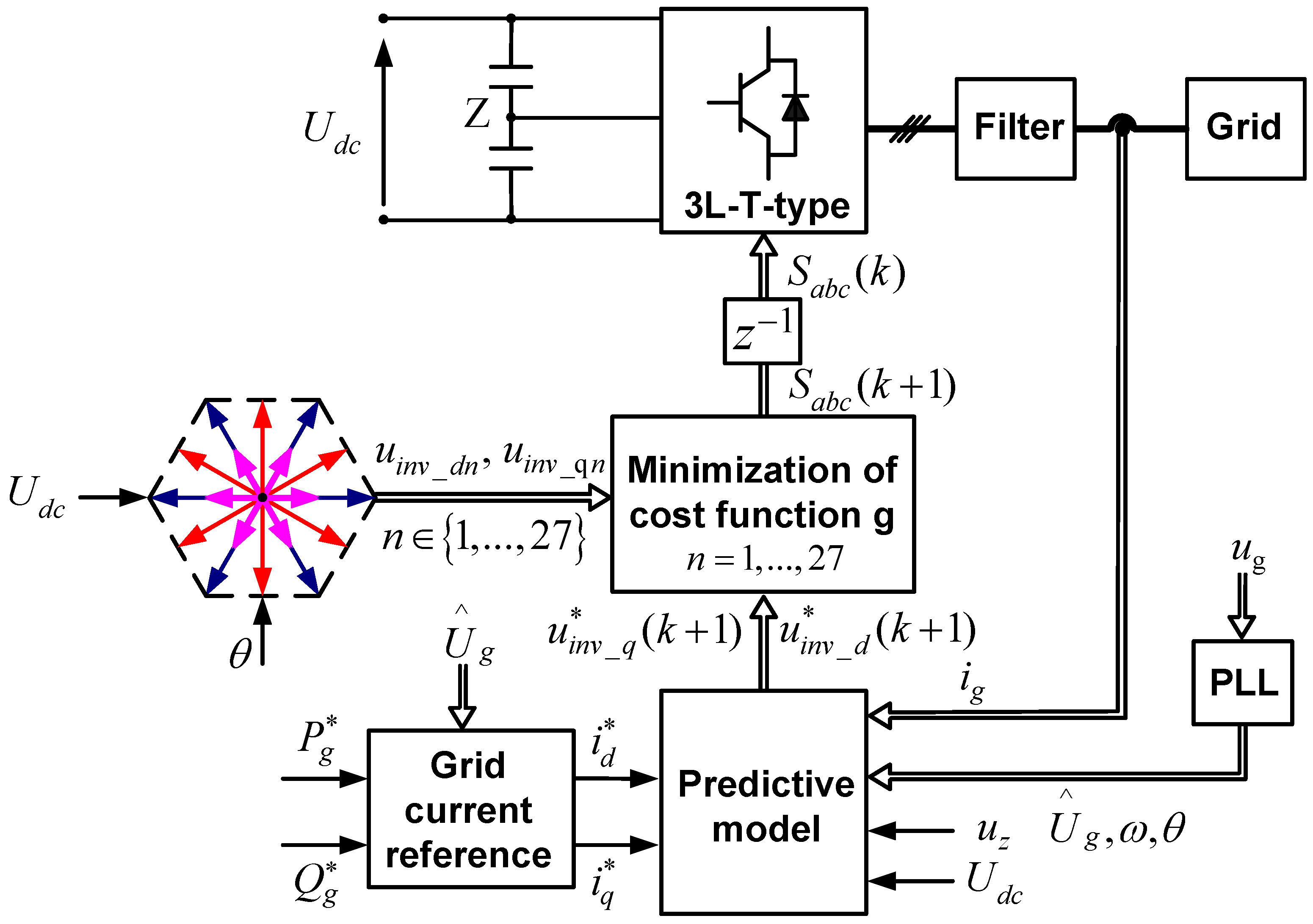
Estimate the grid current: The grid current components ${\widehat{i}}_d(k+1)$ and ${\widehat{i}}_q(k+1)$ at time $k+1$ are evaluated by utilizing Equation (15) with the previous optimal switching state ($u_k$) at time k.

(2)

Calculate the inverter voltage reference: According to Equation (16), the reference components of inverter voltage $u_{inv\_d}^{*}(k+1)$ and $u_{inv\_q}^{*}(k+1)$ at time $k+1$ are calculated in regard to the grid current references $i_d^{*}(k+2)$, $i_q^{*}(k+2)$ at time $k+2$ and estimated grid currents ${\widehat{i}}_d(k+1)$ and ${\widehat{i}}_q(k+1)$ at time $k+1$. Then, the neutral-point voltage at time $k+1$ is computed from grid current $i_g(k)$ and all admissible switching states switching states $u_{k+1}$.

(3)

Evaluate and select the best control input: The optimal control input that has the lowest of the cost function $g_{mdf}$ is implemented at time $k+1$ to the 3L-T-type inverter:

$$\begin{array}{cc}{\widehat{i}}_d(k+1)\hfill & =f_1(i_d(k),i_q(k),u_k),{\widehat{i}}_q(k+1)=f_2(i_q(k),i_d(k),u_k),\hfill \\ u_z^p(k+1)\hfill & =f_3(i_g(k),u_z(k),u_{k+1}),u_{inv\_dn}=f_6(u_{inv\_n});u_{inv\_qn}=f_7(u_{inv\_n}),\hfill \\ u_{inv\_d}^{*}(k+1)\hfill & =f_4(i_d^{*}(k+2),{\widehat{i}}_d(k+1),{\widehat{i}}_q(k+1)),u_{inv\_q}^{*}(k+1)=f_5(i_q^{*}(k+2),{\widehat{i}}_d(k+1),{\widehat{i}}_q(k+1)),\hfill \\ g_{mdf}(u_{k+1})\hfill & =|u_{inv\_d}^{*}(k+1)-u_{inv\_dn}|+|u_{inv\_q}^{*}(k+1)-u_{inv\_qn}|+{\lambda }_{dc}|u_z^p(k+1)|+{\lambda }_{n}s{w}_c,\hfill \\ u_{opt}\hfill & =arg\{\underset{u_{k+1}\in \{-1,0,1{\}}^3}{\min }{g}_{mdf}(u_{k+1})\}.\hfill \end{array}$$

(19)

where $u_{inv\_d}^{*}(k+1)$ and $u_{inv\_q}^{*}(k+1)$ represent the desired inverter voltages at instant $k+1$; and $u_{inv\_dn}$ and $u_{inv\_qn}$ stand for all possible inverter voltage components in $dq$ synchronous reference frame.

It is worth mentioning that there are different terms of the cost function between the traditional MPC and the proposed method as shown in Equations (14) and (19). With the traditional FCS-MPC [25,26,27], all predicted control variables are considered in the optimization loop. In this case, 27 predictive currents $i_d^p(k+2)$ and $i_q^p(k+2)$ are needed to enumerate in the cost function ($g_{cnv}(u_{k+1})$) to obtain the best switching state, which is applied to the inverter at time $k+1$. On the other hand, only one inverter reference voltage $u_{inv}^{*}(k+1)$, which is achieved through the estimated grid current ${\widehat{i}}_g(k+1)$ and grid current reference $i_g^{*}(k+2)$, is taken into account for the loop optimization. Then, by only one evaluating cost function ($g_{mdf}(u_{k+1})$) with simple code optimization, the optimal control input is achieved. Therefore, the proposed technique reduces the computational time of the performance criterion optimization compare with the traditional FCS-MPC. The comparison of computational cost between two controllers is summarized in

Table 2. Comparison of computational cost between two methods.

Variables	Conventional FCS-MPC	Proposed Method
${\widehat{i}}_d(k+1)$, ${\widehat{i}}_q(k+1)$	1	1
$u_{inv\_d}(k+1)$, $u_{inv\_q}(k+1)$	27	27
$i_d^p(k+2)$, $i_q^p(k+2)$	27	0
$u_{inv\_d}^{*}(k+1)$, $u_{inv\_q}^{*}(k+1)$	0	1
$u_z^p(k+1)$	27	27
$s{w}_c$	27	27
Total	109	83

, which highlights the benefit of the proposed method. To validate the efficiency of the proposed algorithm, the function tic-toc in Matlab is used to measure the computation time. Significantly, the minimum, average and maximum values of evaluation time of the conventional FCS-MPC are 17, 29, and 41 $\mathsf{\mu }$s, respectively, and 10, 22, and 34 $\mathsf{\mu }$s for the proposed algorithm, respectively. Figure 4 shows the impact of the computation time in two controllers. This can lead to a 24% reduction of computational complexity, resulting in an increase of sampling frequency for improving the control performance. Consequently, this method has many practical applications for power converters in term of a time-consuming optimization algorithm, thereby supporting the feasibility of real-time applications with low-cost processors. The overall strategy of the proposed control algorithm is illustrated in Figure 5.

Finally, the control objectives are obtained by enumerated the proposed cost function, as demonstrated in Algorithm 1.

Algorithm 1 Algorithm of modified model predictive power control with reduced computational complexity.

Input:$i_g(k),u_z(k),u_g(k),U_{dc}(k),P_g^{*}(k),Q_g^{*}(k)$ Output:$S_a,S_b,S_c$. 1. Estimate the grid current ${\widehat{i}}_{gd}(k+1)$ and ${\widehat{i}}_{gq}(k+1)$ based on (15). 2. Compute the inverter voltage components in the $dq$ synchronous reference frame $u_{inv\_dn}$ and $u_{inv\_qn}$, with $n=1-27$ according to (9). 3. Calculate the grid current references $i_{gd}^{*}(k),i_{gq}^{*}(k)$ and inverter voltage $u_{inv\_d}^{*}(k+1),u_{inv\_q}^{*}(k+1)$ based on (11) and (16). 4. Estimate $s{w}_c$ for all switching states based on (13). 5. Predict the neutral-point voltage $u_z^p(k+1)$ by using (18). 6. Evaluate the cost function $g_{mdf}$ from (19). 7. Select the optimal switching state $x_{opt}$: $[\sim ,x_{opt}]=min(g_{mdf})$; Return to step 1.

4. Simulation and Experimental Results

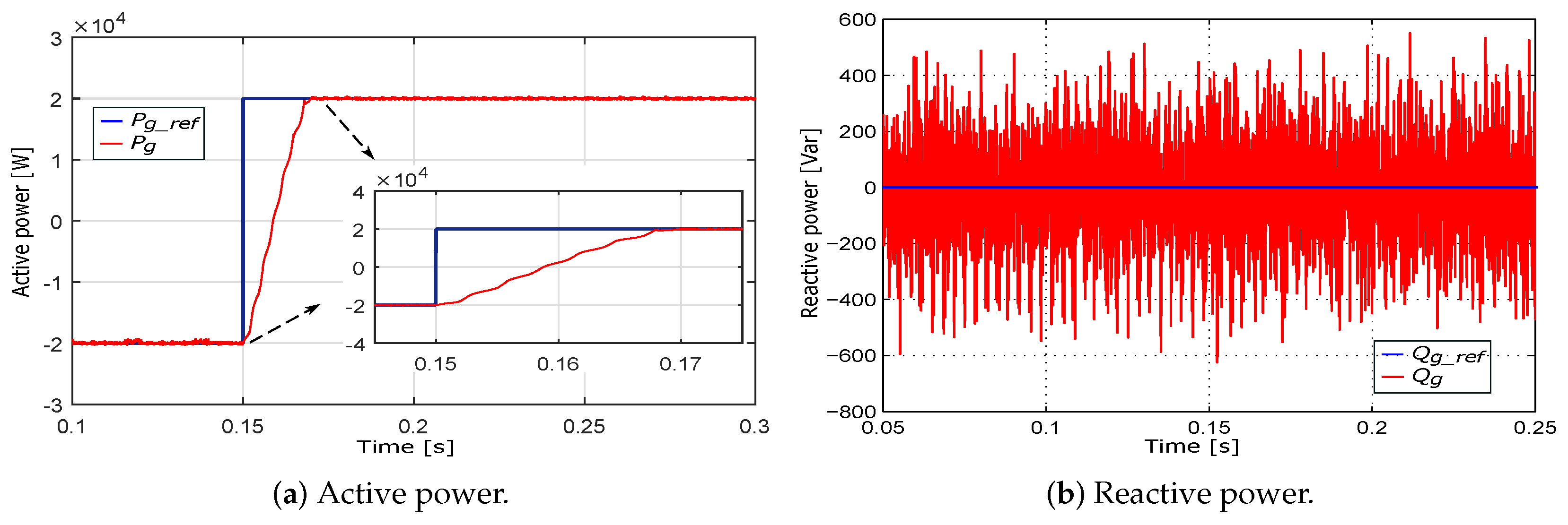
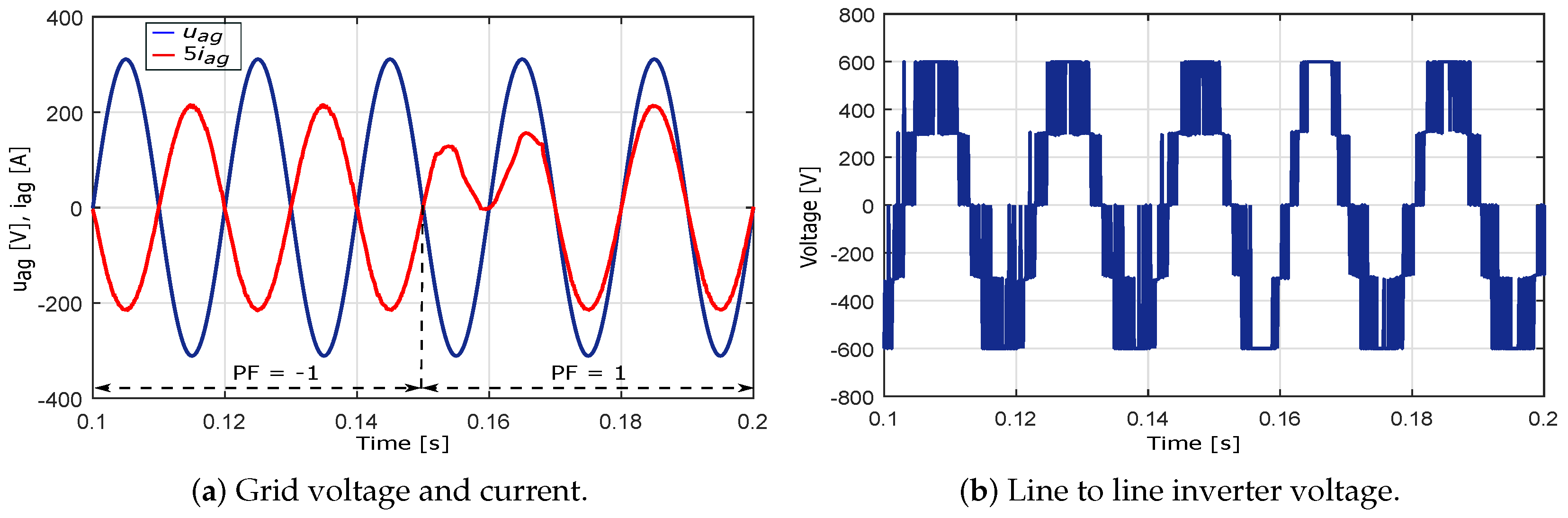
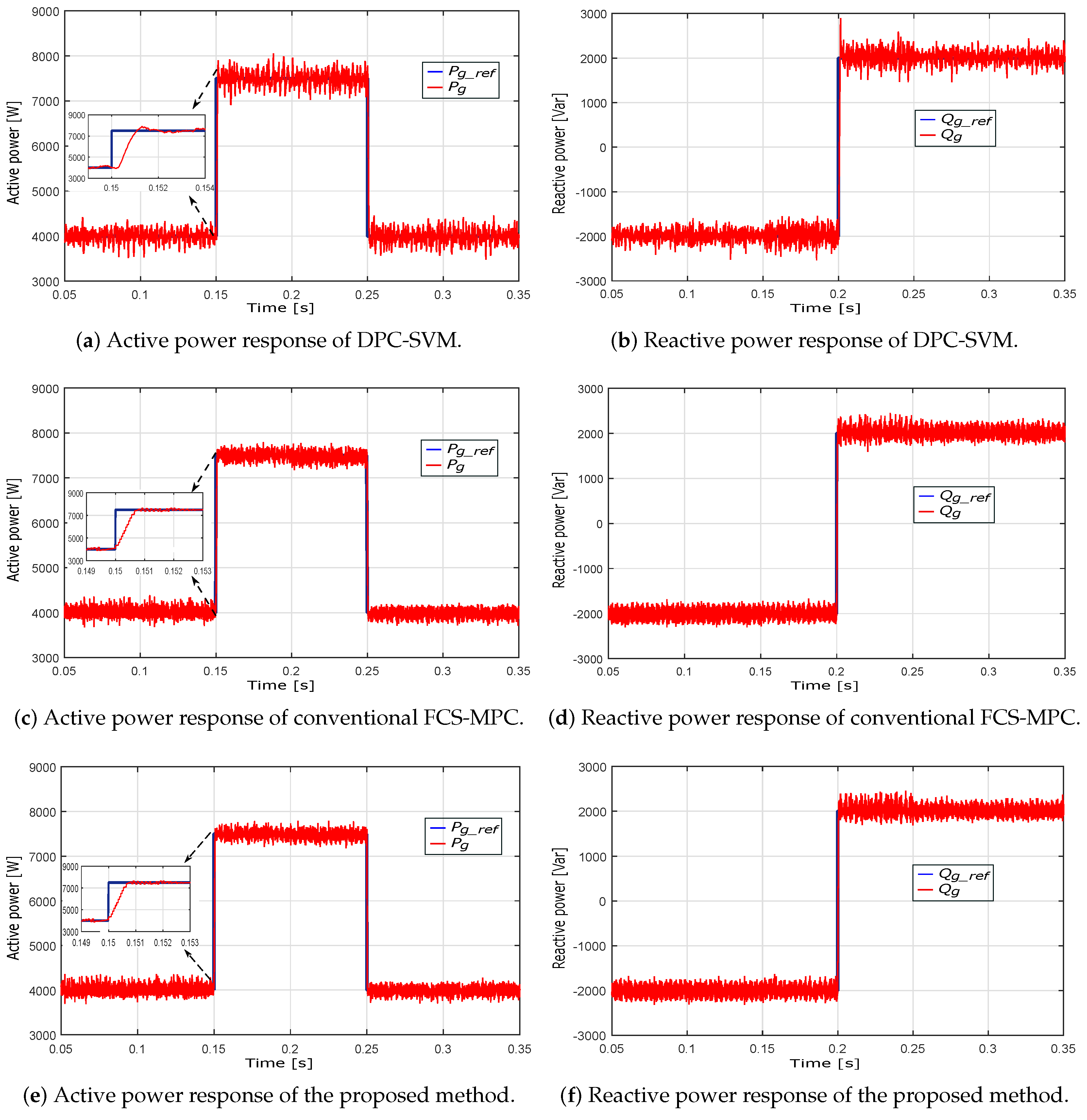
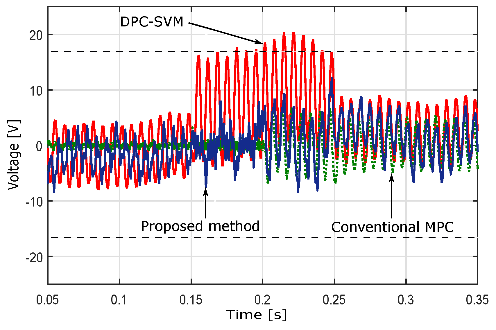
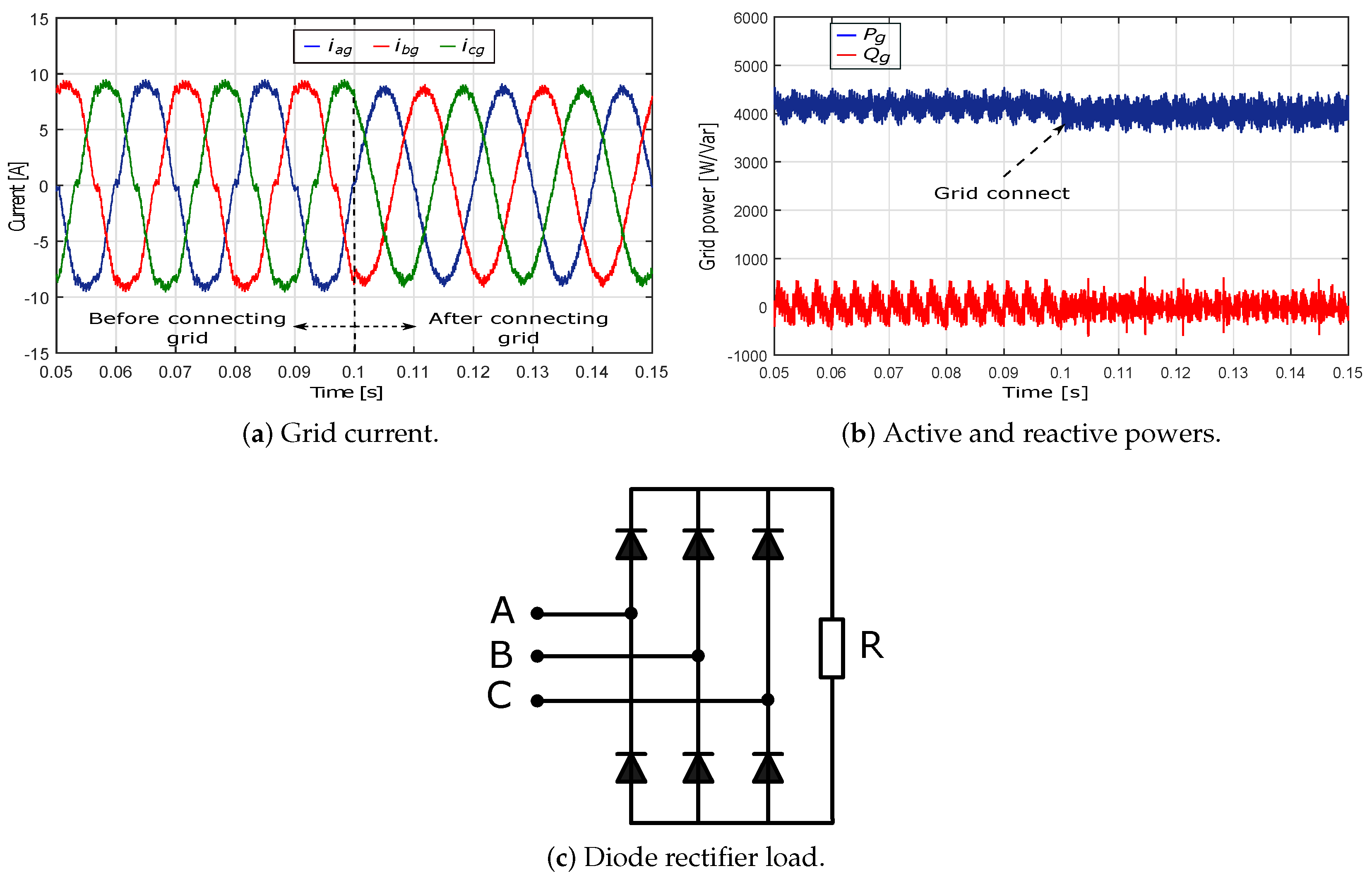
4.1. Simulation Results

To verify the control performance of the proposed control scheme for the grid tie 3L-T-type inverter, examinations were conducted in Matlab/Simulink simulation environment with SimPowerSystems toolbox. The system parameters are as indicated in

Table 3. Simulation parameters.

System Parameters	Value	Representation
$U_{dc}$	600 [V]	DC-bus voltage
$C_{dc}$	1000 [$\mathsf{\mu }$F]	DC-bus capacitance
$R_f$	80 [m$\mathsf{\Omega }$]	Filter resistance
$L_f$	10 [mH]	Filter inductance
$f_s$	20 [kHz]	Sampling frequency of the proposed controller
$f_g$	50 [Hz]	Grid voltage frequency
$U_{dm}$	380 [V]	Grid line-to-line voltage
${\lambda }_{dc}$	20	Weighting factor of the balance of capacitor voltages
${\lambda }_n$	60	Weighting factor of switching frequency

. The control algorithm was implemented by utilizing the Matlab function block.

To evaluate the steady-state control performance, the mean absolute percentage error (MAPE) was used to estimate the power ripple and neutral-point voltage deviation as:

$$MAPE=\frac{1}{n}\sum _{i=1}^n\left|{\displaystyle \frac{y_i^{*}-y_i}{y_i^{*}}}\right|,$$

(20)

where $y_i^{*}$ and $y_i$ are the reference and measurement vectors, respectively.

To calculate the average switching frequency of the inverter achieved by the FCS-MPC, the following expression suggested in [27] can be used:

$$f_{sw}=\sum _{x=a,b,c}\frac{n_{s{w}_{1x}}+n_{s{w}_{2x}}+n_{s{w}_{3x}}+n_{s{w}_{4x}}}{12T_{sim}},$$

(21)

where $n_{s{w}_{1x}}$, $n_{s{w}_{2x}}$, $n_{s{w}_{3x}}$ and $n_{s{w}_{4x}}$ denote the number of commutations of each leg in the time interval ($T_{sim}$).

In the first scenario, the proposed method was performed to demonstrate the ability of the bidirectional transmitted power with a unity power factor ($Q_{g\_ref}=0$ Var). The reference of power factor (PF) changed from −1 to 1 at $t=0.15$ s, corresponding to a step change of active power $P_{g\_ref}$ from −20 kW to 20 kW. In the inverting mode operation ($P_g<0$), the active power was supplied to the grid, whereas the power was absorbed from the grid with rectifying mode operation ($P_g>0$). As shown in Figure 6, the proposed method enhanced a fast steady-state and high control performance. The phase difference between the grid voltage and current is depicted in Figure 7a. Figure 7b shows the variable switching frequency of inverter output voltage. However, this does not impact too much the control performance.

In the second scenario, the control system was conducted with different values of active and reactive powers. To confirm the effectiveness of the control scheme, a comparative analysis was carried out among the proposed method, conventional FCS-MPC [27] and direct power control with PI controllers [11]. This linear controller employs the redundant states to keep the DC-bus capacitor voltage balancing [6]. The sampling frequency of the MPC and DPC-SVM is considered $f_s=20$ kHz and 6 kHz, respectively, to produce the equivalent average switching frequency $f_{sw}=3$ kHz. The reference of active and reactive powers were set at 4 kW and −2 kVar, according to the $PF=-0.89$. The active power reference ($P_{g-ref}$) was stepped from 4 kW to 7.5 kW at $t=0.15$ s, and then back to 4 kW at instant $t=0.25$ s. The active power reference and its measured value are demonstrated in Figure 8a. A step change in required reactive power $Q_{g-ref}$) from −2 kVar to 2 kVar at $t=0.2$ corresponded to leading power factor and lagging power factor, respectively, as illustrated in Figure 8b. The results shown in Figure 8 prove that the proposed method enhanced the dynamic performance with no overshoot compared to the DPC-SVM, as confirmed in

Table 4. Comparative studies of transient performance for three controllers.

Active Power Step	${\mathit{P}}_{\mathit{g}}^{*}$ = 4 → 7.5 (kW)
	DPC-SVM	Conventional FCS-MPC	Proposed Method
Rise time (ms)	1.1	0.8	0.8
Settling time (ms)	4.8	0.8	0.8
Overshoot (%)	5.3	0	0
THD of grid current (%)	3.2	2.51	2.5

. In fact, the active power of the conventional MPC and proposed method reached steady-state of the transient response from 4 kW to 7.5 kW in about 0.8 ms and 1.1 ms with DPC-SVM, respectively. The MAPE of the active power of the proposed method reduced from 5.22% to 3.75%, and from 11.03% to 7.98% with reactive power, compared with DPC-SVM.

Figure 9 demonstrates the dynamic response and grid current harmonic spectra using the Powergui fast Fourier transform (FFT) toolbox. The results in Figure 9 indicate the advantages of the proposed control method. It was observed that the total harmonic distortion (THD) of the grid current at $t=0.18$ s for the proposed method (2.5%) was better than DPC-SVM (3.2%). Particularly, the proposed method accomplished a similar current performance compared with the traditional FCS-MPC, as shown in Figure 9c,e. Moreover, the THD of the grid current was not only decreased but was also less time-consuming. It means that the control algorithm proved the advantage of the proposed method in terms of computation load. Consequently, it is fundamental to underline that the proposed method represents a useful alternative to implementing MPC algorithm in a real-time system.

In addition, the proposed method can solve the drawback of unbalancing DC-link capacitor voltage, as shown in Figure 10. It is interesting to note that the DC-link capacitor voltages remained balanced with MAPE of neutral-point voltage deviation for the proposed method of 0.48% and 0.93% with DPC-SVM.

To analyze the influence of the non-linear load, a study with diode rectifier and resistive load ($R=60\mathsf{\Omega }$) was investigated, as illustrated in Figure 11c. The active and reactive powers were set at 4 kW and 0 Var, respectively. Figure 11 demonstrates the results with stand-alone and grid-connected modes at $t=0.1$ s. As shown in Figure 11a,b, the ripples of the grid current and powers were increased in the standard-alone mode. However, the grid current remained sinusoidal after connecting to the grid. Moreover, the active and reactive powers continued tracking their reference values with a fast transient time. Therefore, i the proposed method could adopt a non-linear load.

The selection of the weighting factor is not a transparent task for FCS-MPC, but this issue can be addressed by using the multi-objective optimization techniques suggested by Cortes et al. [33]. The unbalance of DC-bus capacitor voltage is guaranteed by a high value of ${\lambda }_{dc}$, but it augments the power ripples and the THD of the grid current. The criteria for selecting ${\lambda }_{dc}$ is the neutral-point voltage deviation, which is considered about 3% of DC-bus voltage, as depicted in Figure 10. On the contrary, the switching frequency was reduced by increasing the weighting factor ${\lambda }_n$, resulting in switching loss reduction. However, the augmentation of the THD of grid current and power ripple also occurred as a result of the weighting factor ${\lambda }_n$. Recognizing the THD as a key to estimate the performance, a satisfactory weighting factor can be achieved by increasing its value in a simulation environment. When the weighting factor ${\lambda }_n$ changed from 0 to 120, the switching frequency $f_{sw}$ decreased from 4197 to 2049 Hz, corresponding to the increment in active power error (Figure 12b) and THD of the grid current from 4.02% to 15.55% and from 2.28% to 9.17%, respectively (Figure 12a). As a result, the weighting factor ${\lambda }_{dc}$ and ${\lambda }_n$ can be selected at 20 and 60 to obtain an adequate control performance with the low THD, the DC-bus capacitor voltage balancing and the switching frequency device at 3 kHz.

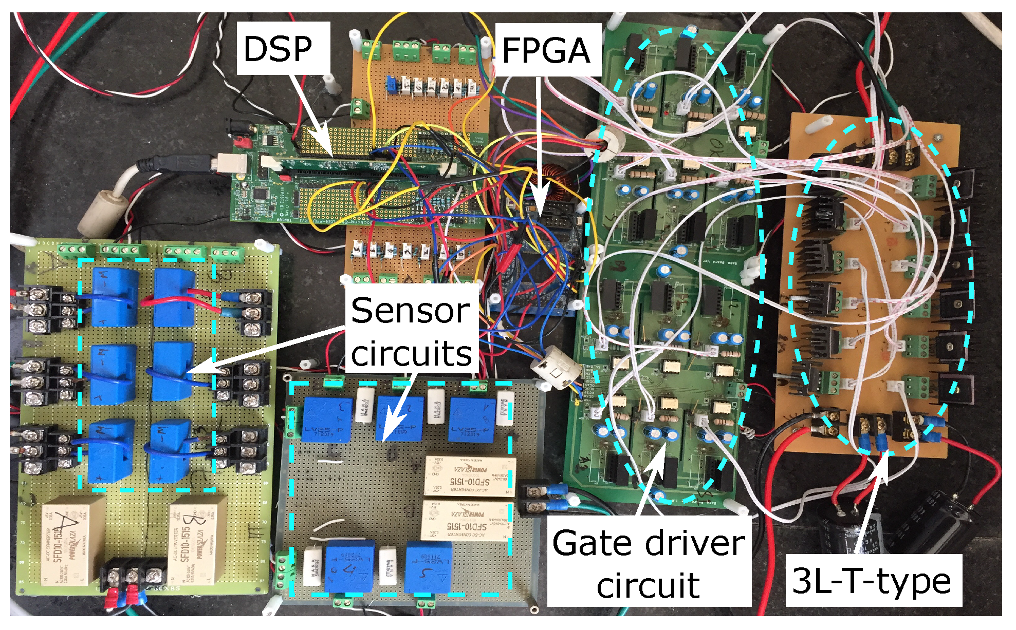
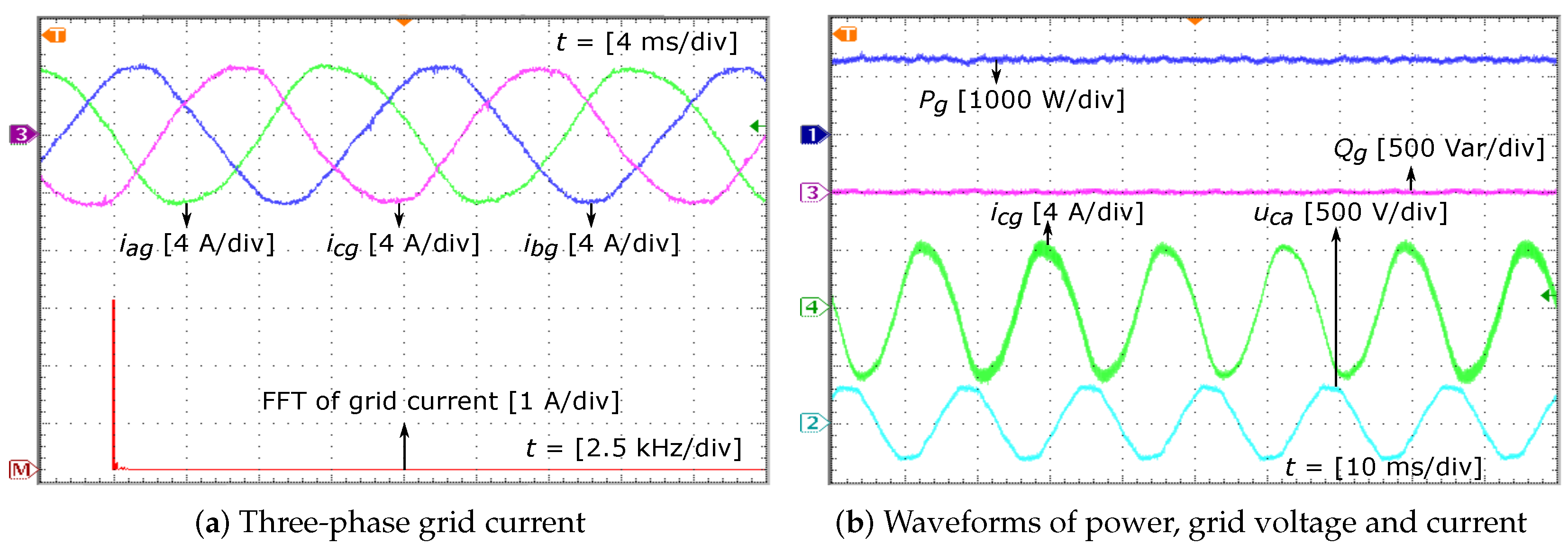
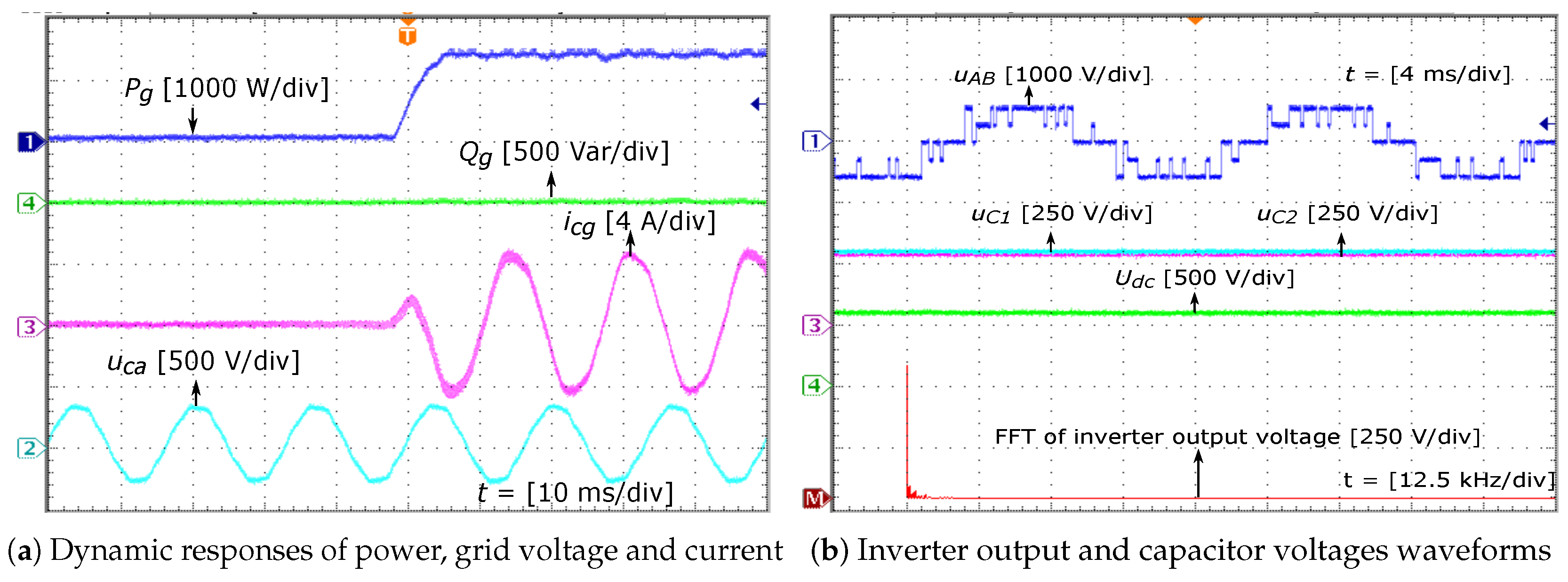
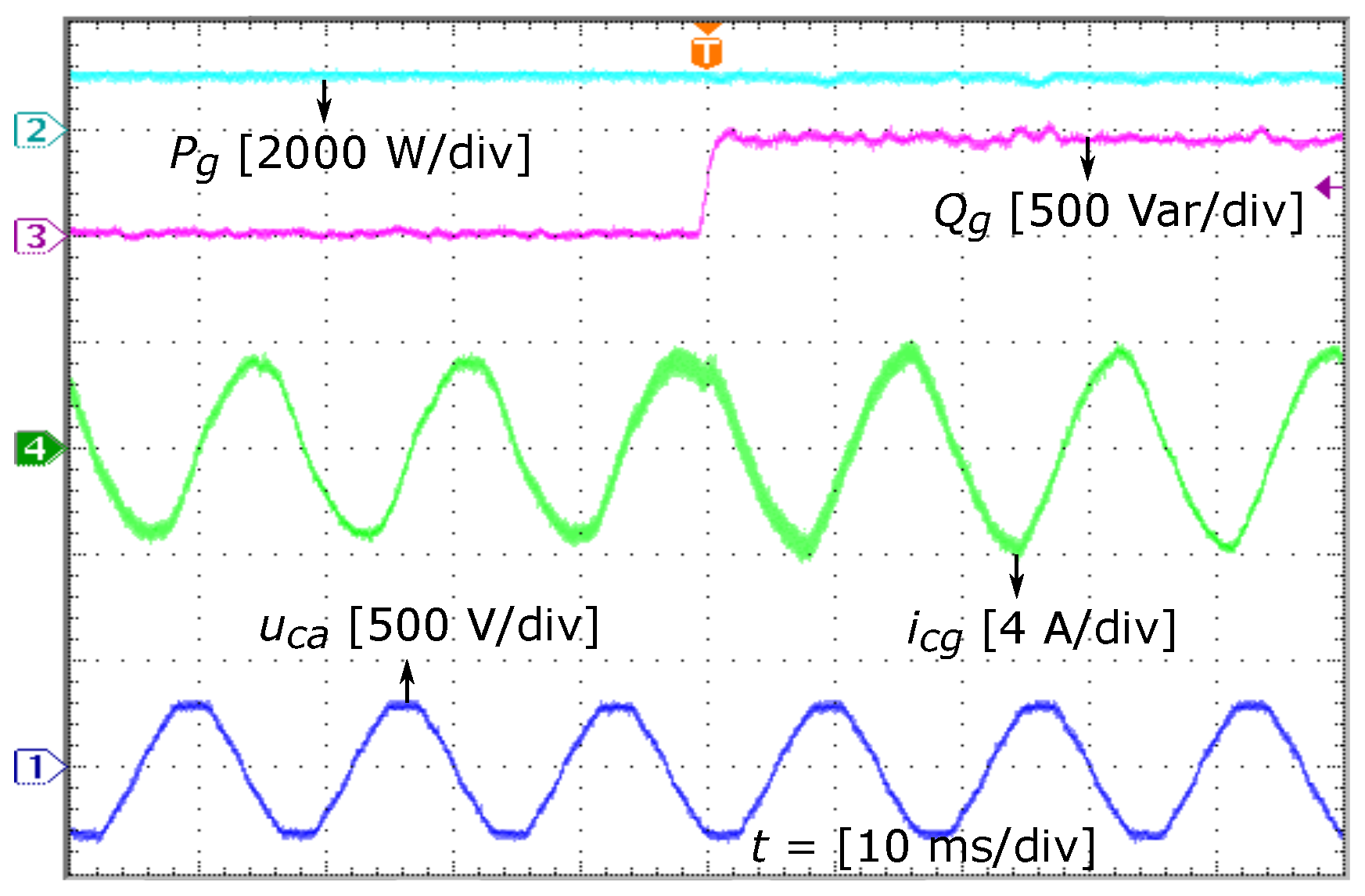
4.2. Experimental Results

With the purpose of verifying the benefit of the proposed control strategy such as rapid dynamic transient, reasonable THD of the grid current and reduced execution time, a scale down prototype was built in the laboratory, as illustrated in Figure 13. The control algorithm was implemented in a digital signal processing (DSP) TMS320F28335 controller by using the S-function builder block in Matlab/Simulink environment. Twelve FGH40T120SMD IGBT modules were employed for the inverter. Moreover, DC-link used two capacitors LGG2G102MELC50 1000 $\mathsf{\mu }$F-400 V for the test bench. The parameters of the filter remained the same as in the simulation. The capacitor voltage, grid voltage, and current were measured by LV 25-P and LA 25-P transducers. The switch signals were generated by general-purpose input/output (GPIO) outputs of the DSP.

The DC-link voltage was fixed at 600 V while the root mean squared and frequency of the grid voltage remained at 220 V and 60 Hz, respectively. The sampling time of the proposed control method was 100 $\mathsf{\mu }$s, which is suitable for low-speed processing of DSP. The stable and dynamic transient states were examined with the change in the active and reactive powers to confirm the feasibility of the proposed control. In the first scenario, Figure 14 illustrates the steady-state performance of the proposed control strategy with active power $P_g=1300$ W and unity power factor ($Q_g=0$ Var). The experimental results indicate that the ability to track power and achieved sinusoidal grid current waveform. In this test, the three-phase grid voltage was not a good sinusoidal waveform, as shown in Figure 14b, leading to a decrease in the quality of the grid current.

In the second scenario, two cases of the step change in the active and reactive powers were investigated to validate the ability tracking behavior of the proposed control scheme. In the first case, the active power reference was changed from 0 to 1300 W according to the change in grid current from 0 to 4.2 A. As shown in Figure 15, the active power and grid current reached the steady-state after a short transient time. Furthermore, the voltage-balancing of DC-bus capacitors and the reactive power were guaranteed even under the transient response. In the second case, the active power reference was kept at 1000 W while the reference of reactive power was stepped from 0 to 436 Var. It is apparent from the results in Figure 16 that the proposed approach obtained an accurate power tracking capacity under the change of the power factor.

Two controllers had the same performance of the THD for the grid current, as depicted in Figure 17. The THD of the grid current for the proposed method was 3.4% and 3.5% with the conventional FCS-MPC. Moreover, the execution time of the control strategy for the proposed method decreased from 88 to 69 $\mathsf{\mu }$s in comparison to the traditional FCS-MPC, as illustrated in Figure 18. This underlined the 22% reduction of execution time with the proposed method. Although, with the development of the microcontrollers, the execution time can be decreased by using the fast DSP or FPGA, this means that the cost of the system is increased, which becomes a challenge in industrial applications. Consequently, our study provides additional support to implement the MPC algorithm with the low-cost processor.

5. Conclusions

This paper presents a development power control strategy based on model predictive control for grid-tie 3L-T-type inverter while ensuring DC-bus capacitor voltage balancing and reduction of switching frequency. Moreover, the inverter voltage reference is applied to compute the equivalent cost function for determining the best control input, leading to reduce the computational effort compared with the conventional FCS-MPC method. A comparison study indicated that the proposed method achieves high-performance control of power and low THD of the current compared with the classical DPC-SVM. Simulations and experiments verified and highlighted the effectiveness of the proposed method.

References

1. Blaabjerg, F.; Liserre, M.; Ma, K. Power Electronics Converters for Wind Turbine Systems. IEEE Trans. Ind. Appl. 2012, 48, 708–719. [Google Scholar] [CrossRef]
2. Portillo, R.C.; Prats, M.M.; Leon, J.I.; Sanchez, J.A.; Carrasco, J.M.; Galvan, E.; Franquelo, L.G. Modeling Strategy for Back-to-Back Three-Level Converters Applied to High-Power Wind Turbines. IEEE Trans. Ind. Electron. 2006, 53, 1483–1491. [Google Scholar] [CrossRef]
3. Kouro, S.; Malinowski, M.; Gopakumar, K.; Pou, J.; Franquelo, L.G.; Wu, B.; Rodriguez, J.; Perez, M.A.; Leon, J.I. Recent Advances and Industrial Applications of Multilevel Converters. IEEE Trans. Ind. Electron. 2010, 57, 2553–2580. [Google Scholar] [CrossRef]
4. Schweizer, M.; Kolar, J.W. Design and Implementation of a Highly Efficient Three-Level T-Type Converter for Low-Voltage Applications. IEEE Trans. Power Electron. 2013, 28, 899–907. [Google Scholar] [CrossRef]
5. Qin, C.; Zhang, C.; Chen, A.; Xing, X.; Zhang, G. A Space Vector Modulation Scheme of the Quasi-Z-Source Three-Level T-Type Inverter for Common-Mode Voltage Reduction. IEEE Trans. Ind. Electron. 2018, 65, 8340–8350. [Google Scholar] [CrossRef]
6. Wu, B.; Narimani, M. High-Power Converters and AC Drives; Wiley-IEEE Press: Piscataway, NJ, USA, 2017. [Google Scholar]
7. Ngo, B.Q.V.; Ayerbe, P.R.; Olaru, S. Model Predictive Control with Two-step horizon for Three-level Neutral-Point Clamped Inverter. In Proceedings of the 20th International Conference on Process Control, Strbske Pleso, Slovakia, 9–12 June 2015; pp. 215–220. [Google Scholar]
8. Kang, J.W.; Hyun, S.W.; Ha, J.O.; Won, C.Y. Improved Neutral-Point Voltage-Shifting Strategy for Power Balancing in Cascaded NPC/H-Bridge Inverter. Electronics 2018, 7, 167. [Google Scholar] [CrossRef]
9. Vahedi, H.; Labbe, P.A.; Al-Haddad, K. Balancing three-level NPC inverter DC bus using closed-loop SVM Real time implementation and investigation. IET Power Electron. 2016, 9, 2076–2084. [Google Scholar] [CrossRef]
10. In, H.C.; Kim, S.M.; Lee, K.B. Design and Control of Small DC-Link Capacitor-Based Three-Level Inverter with Neutral-Point Voltage Balancing. Energies 2018, 11, 1435. [Google Scholar] [CrossRef]
11. Wilamowski, B.M.; Irwin, J.D. Power Electronics and Motor Drives; Taylor and Francis Group: Oxfordshire, UK, 2011. [Google Scholar]
12. Gui, Y.; Lee, G.H.; Kim, C.; Chung, C.C. Direct power control of grid connected voltage source inverters using port-controlled Hamiltonian system. Int. J. Control Autom. Syst. 2017, 15, 2053–2062. [Google Scholar] [CrossRef]
13. Zorig, A.; Belkheiri, M.; Barkat, S. Control of three-level T-type inverter based grid connected PV system. In Proceedings of the 13th International Multi-Conference on Systems, Signals & Devices, Leipzig, Germany, 21–24 March 2016; pp. 66–71. [Google Scholar]
14. Hernández, J.C.; Sanchez-Sutil, F.; Vidal, P.G.; Rus-Casas, C. Primary frequency control and dynamic grid support for vehicle-to-grid in transmission systems. Int. J. Electr. Power Energy Syst. 2018, 100, 152–166. [Google Scholar] [CrossRef]
15. Hernandez, J.C.; Bueno, P.G.; Sanchez-Sutil, F. Enhanced utility-scale photovoltaic units with frequency support functions and dynamic grid support for transmission systems. IET Renew. Power Gener. 2017, 11, 361–372. [Google Scholar] [CrossRef]
16. Bueno, P.G.; Hernández, J.C.; Ruiz-Rodriguez, F.J. Stability assessment for transmission systems with large utility-scale photovoltaic units. IET Renew. Power Gener. 2016, 10, 584–597. [Google Scholar] [CrossRef]
17. Malinowski, M.; Kazmierkowski, M.P.; Hansen, S.; Blaabjerg, F.; Marques, G.D. Virtual-flux-based direct power control of three-phase PWM rectifiers. IEEE Trans. Ind. Appl. 2001, 37, 1019–1027. [Google Scholar] [CrossRef]
18. Song, Z.; Tian, Y.; Yan, Z.; Chen, Z. Direct Power Control for Three-Phase Two-Level Voltage-Source Rectifiers Based on Extended-State Observation. IEEE Trans. Ind. Electron. 2016, 63, 4593–4603. [Google Scholar] [CrossRef]
19. Sebaaly, F.; Vahedi, H.; Kanaan, H.Y.; Moubayed, N.; Al-Haddad, K. Design and Implementation of Space Vector Modulation-Based Sliding Mode Control for Grid-Connected 3L-NPC Inverter. IEEE Trans. Ind. Electron. 2016, 63, 7854–7863. [Google Scholar] [CrossRef]
20. Scoltock, J.; Geyer, T.; Madawala, U.K. Model Predictive Direct Power Control for Grid-Connected NPC Converters. IEEE Trans. Ind. Electron. 2015, 62, 5319–5328. [Google Scholar] [CrossRef]
21. Vazquez, S.; Marquez, A.; Aguilera, R.; Quevedo, D.; Leon, J.I.; Franquelo, L.G. Predictive Optimal Switching Sequence Direct Power Control for Grid-Connected Power Converters. IEEE Trans. Ind. Electron. 2015, 62, 2010–2020. [Google Scholar] [CrossRef]
22. Ngo, V.Q.B.; Nguyen, M.K.; Tran, T.T.; Lim, Y.C.; Choi, J.H. A Simplified Model Predictive Control for T-Type Inverter with Output LC Filter. Energies 2019, 12, 31. [Google Scholar] [CrossRef]
23. Donoso, F.; Mora, A.; Cárdenas, R.; Angulo, A.; Sáez, D.; Rivera, M. Finite-Set Model-Predictive Control Strategies for a 3L-NPC Inverter Operating With Fixed Switching Frequency. IEEE Trans. Ind. Electron. 2018, 65, 3954–3965. [Google Scholar] [CrossRef]
24. Ngo, B.Q.V.; Rodriguez-Ayerbe, P.; Olaru, S.; Niculescu, S.I. Model predictive power control based on virtual flux for grid connected three-level neutral-point clamped inverter. In Proceedings of the 18th European Conference on Power Electronics and Applications, Karlsruhe, Germany, 5–9 September 2016; pp. 1–10. [Google Scholar]
25. Kouro, S.; Cortes, P.; Vargas, R.; Ammann, U.; Rodriguez, J. Model Predictive Control: A Simple and Powerful Method to Control Power Converters. IEEE Trans. Ind. Electron. 2009, 56, 1826–1838. [Google Scholar] [CrossRef]
26. Rodriguez, J.; Kazmierkowski, M.P.; Espinoza, J.R.; Zanchetta, P.; Abu-Rub, H.; Young, H.A.; Rojas, C.A. State of the Art of Finite Control Set Model Predictive Control in Power Electronics. IEEE Trans. Ind. Inform. 2013, 9, 1003–1016. [Google Scholar] [CrossRef]
27. Rodriguez, J.; Cortes, P. Predictive Control of Power Converters and Electrical Drives; John Wiley & Sons, Inc.: New York, NY, USA, 2012. [Google Scholar]
28. Shi, T.; Zhang, C.; Geng, Q.; Xia, C. Improved model predictive control of three-level voltage source converter. Electr. Power Compon. Syst. 2014, 42, 1029–1138. [Google Scholar] [CrossRef]
29. Geyer, T.; Quevedo, D.E. Performance of Multistep Finite Control Set Model Predictive Control for Power Electronics. IEEE Trans. Power Electron. 2015, 30, 1633–1644. [Google Scholar] [CrossRef]
30. Aguilera, R.P.; Baidya, R.; Acuna, P.; Vazquez, S.; Mouton, T.; Agelidis, V.G. Model predictive control of cascaded H-bridge inverters based on a fast-optimization algorithm. In Proceedings of the 41st Annual Conference of the IEEE Industrial Electronics Society, Yokohama, Japan, 9–12 November 2015; pp. 4003–4008. [Google Scholar]
31. Xia, C.; Liu, T.; Shi, T.; Song, Z. A Simplified Finite-Control-Set Model-Predictive Control for Power Converters. IEEE Trans. Ind. Inform. 2014, 10, 991–1002. [Google Scholar]
32. Taheri, A.; Zhalebaghi, M.H. A new model predictive control algorithm by reducing the computing time of cost function minimization for NPC inverter in three-phase power grids. ISA Trans. 2017, 71, 391–402. [Google Scholar] [CrossRef] [PubMed]
33. Cortes, P.; Kouro, S.; Rocca, B.L.; Vargas, R.; Rodriguez, J.; Leon, J.I.; Vazquez, S.; Franquelo, L.G. Guidelines for weighting factors design in Model Predictive Control of power converters and drives. In Proceedings of the 2009 IEEE International Conference on Industrial Technology, Gippsland, VIC, Australia, 10–13 February 2009; pp. 1–7. [Google Scholar]
Figure 1. Simplified configuration of the grid-connected 3L-T-type inverter.
Electronics 08 00217 g001
Figure 2. Coordinate reference system.
Electronics 08 00217 g002
Figure 3. Control variable of one-step horizon with delay compensation.
Electronics 08 00217 g003
Figure 4. Computation time of two controllers.
Electronics 08 00217 g004
Figure 5. Block diagram of the proposed control scheme.
Electronics 08 00217 g005
Figure 6. The transient power responses for a step in active power reference with a unity power factor.
Electronics 08 00217 g006
Figure 7. Inverter output voltage and grid voltage and current waveforms.
Electronics 08 00217 g007
Figure 8. The transient responses of active and reactive powers.
Electronics 08 00217 g008
Figure 9. The dynamic response and harmonic spectrum of the grid current for DPC-SVM, conventional FCS-MPC, and the proposed method.
Electronics 08 00217 g009
Figure 10. Performance of the neutral-point voltage u z .
Electronics 08 00217 g010
Figure 11. Grid current and power responses with the non-linear load.
Electronics 08 00217 g011
Figure 12. Weighting factor impact on: (a) the THD of the grid current and switching frequency; and (b) the power ripple.
Electronics 08 00217 g012
Figure 13. Experimental prototype in the laboratory.
Electronics 08 00217 g013
Figure 14. Experimental results of the proposed method in steady-state with P g = 1300 W and Q g = 0 Var.
Electronics 08 00217 g014
Figure 15. Experimental results of the step change in active power from 0 to 1300 W with Q g = 0 Var.
Electronics 08 00217 g015
Figure 16. Transient response of the step change in reactive power from 0 to 436 Var with P g = 1000 W.
Electronics 08 00217 g016
Figure 17. THD of grid current.
Electronics 08 00217 g017
Figure 18. Execution time of the control strategy for the conventional FCS-MPC and proposed methods.
Electronics 08 00217 g018