Optimization Algorithm for Multiple Phases Sectionalized Modulation Jamming Based on Particle Swarm Optimization

Abstract

Due to the difficulty in deducing the corresponding relationship between results and parameter settings of multiple phases sectionalized modulation (MPSM) jamming, a problem occurs when obtaining the optimal local suppression jamming effect, which limits the practical application of MPSM jamming. The traditional method struggles to meet the requirements by setting fixed parameters or random parameters. Therefore, an optimization algorithm for MPSM jamming based on particle swarm optimization (PSO) is proposed in this study to produce the optimal local suppression jamming effect and determine its corresponding parameter settings. First, we analyzed the relationship between the degree of mismatch and local suppression jamming effect. Then, we set appropriate fitness function and fitness value. Finally, we used PSO to calculate parameter settings of a section situation and phase situation, which minimizes the fitness function and fitness value. The optimization algorithm avoids the tremendous computation of traversing all parameter settings, is stable, the results are repeatable, and the algorithm provides the optimal local suppression jamming effect under different conditions. The simulation experiments demonstrate the feasibility and effectiveness of the optimization algorithm.

1. Introduction

With the development of electronic information technology, radars are playing an increasingly important role in the military field. Modern war has evolved from the traditional competition for air and sea power to the competition for information and electromagnetic spectrum power, which is called electronic warfare (EW). EW usually includes three aspects: electronic support (ES), electronic attack (EA), and electronic protection (EP). The main purpose of EA is to destroy the enemy’s use of the electromagnetic spectrum and seize control of information and the electromagnetic spectrum. Jamming is the most important means of EA. However, linear frequency modulation (LFM) signal and pulse compression, which enhance the radar anti-jamming capability and increase the difficulty of jamming, are widely used in modern radar [1,2]. Therefore, research on jamming techniques and their optimization is becoming increasingly significant.

According to the jamming effect, jamming can be divided into deception jamming and suppression jamming. Deception jamming, by emitting false signals that are highly similar to real signals and confusing to the enemy [3], requires a large amount of information on radar parameter settings that are crucial to the deceptive effect [4]. When there are slight errors in the reconnaissance of parameter settings, deception jamming will be detected and eliminated with a high probability due to the quick decrease in the deceptive effect [5]. Suppression jamming, by blanketing real signals with high-power noise signals and destroying the enemy’s ability to obtain information, requires less information on parameter settings, making suppression jamming a better choice when there is limited information and local suppression is required [6,7].

Traditional suppression jamming, such as radio frequency noise jamming, noise amplitude modulation jamming, and noise frequency modulation jamming [8], can produce a wide range of suppression jamming effects, but cannot obtain a process gain from pulse compression because of its non-coherence. Without process gain, traditional suppression jamming always needs extremely high power to maintain an effective suppression effect. The wide range of suppression jamming effects requires large amounts of jamming power. Traditional suppression jamming is limited by some anti-jamming measures, such as clipping technology and adaptive nulling technology. All these weaknesses make traditional suppression jamming increasingly difficult to apply in various situations.

Modern suppression jamming, which has been a research hotspot, is generated by modulating the received radar signals with different parameters and methods. Therefore, modern suppression jamming can obtain a process gain and reduce jamming power because of its coherence [9]. According to different modulations, there are many kinds of suppression jamming, such as noise convolution jamming [10,11,12,13,14,15,16] and scattered wave jamming [17,18,19,20,21,22]. Noise convolution jamming, which is also called smart jamming, is generated by convoluting received radar signal and noise signal. Noise convolution jamming can produce different local suppression jamming effects according to the noise signal, but its calculation is relatively complicated and resource-consuming. Scattered wave jamming, which is the echo signal emitted from the jammer to the surface, can obtain the real target’s information. However, its control requires relatively high precision.

Multiple phases sectionalized modulation (MPSM) jamming, which is generated by modulating different phases in different sections of the received radar signal, is a kind of coherent suppression jamming with a range-controllable local suppression jamming effect [23,24]. MPSM jamming is a kind of coherent suppression jamming with process gain and simple modulation, which makes MPSM jamming a better choice for coherent suppression jamming. However, deducing the corresponding relationship between results and parameter settings of MPSM jamming is difficult, which means that the optimal local suppression jamming effect of MPSM jamming cannot be obtained from mathematical calculation.

To solve this problem, an optimization algorithm based on particle swarm optimization (PSO) is proposed in this study to obtain the optimal local suppression jamming effect and its corresponding parameter settings. We first model and analyze the principle of MPSM jamming. Next, the influence of section situation and phase situation are studied. Then, the algorithm based on PSO is proposed and designed. Finally, the feasibility and effectiveness of the optimization algorithm are verified by simulation experiments.

2. Principle of MPSM Jamming

2.1. MPSM Jamming Modeling

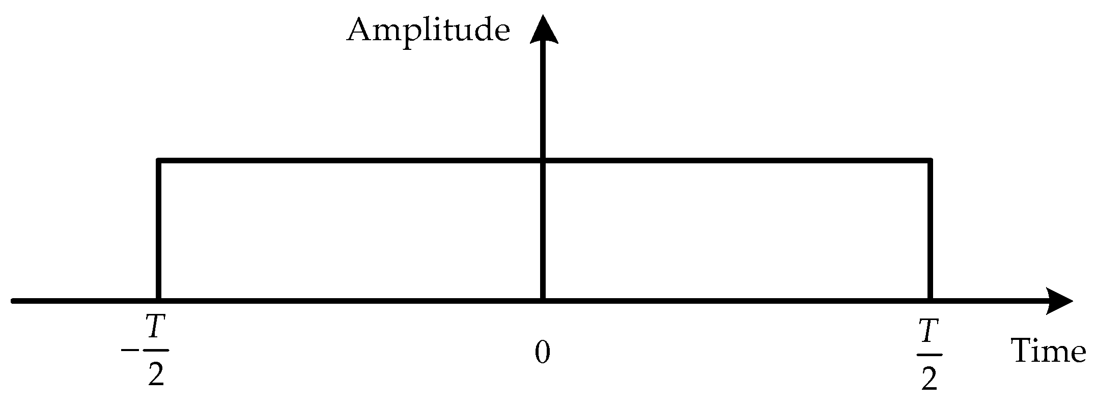
Assume that the received radar signal is x(t), the pulse width of $x\left(t\right)$ is $T$, the envelope is a rectangular envelope, and the envelope center is at zero point of coordinate axis, which means that the beginning time of $x\left(t\right)$ is $-T/2$, and the ending time is $T/2$, as shown in Figure 1.

$$x(t)=rect\left(\frac{t}{T}\right)$$

(1)

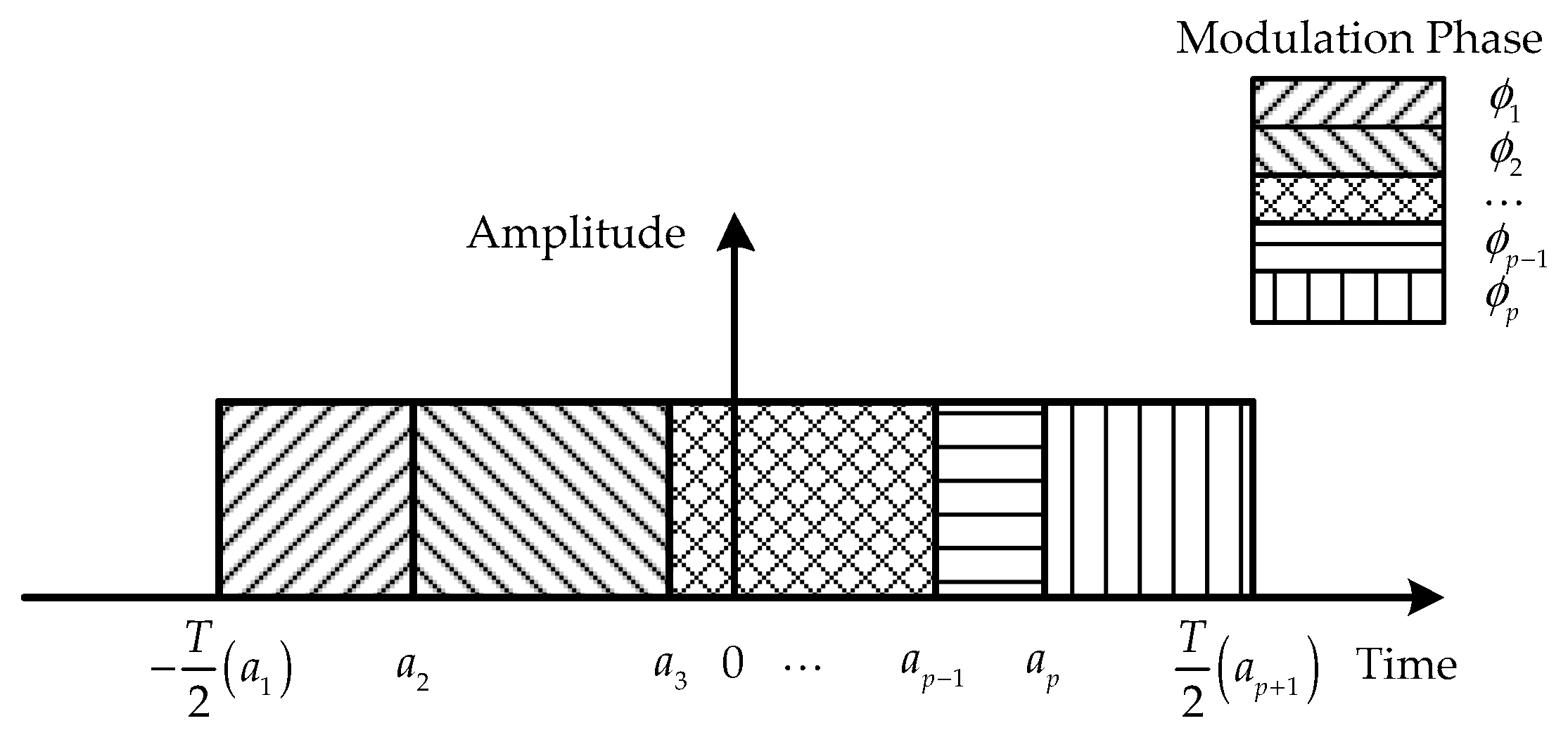
MPSM jamming divides the received radar signal into $p$ sections in time domain, where the length of each section could be equal or unequal, and modulates phase ${\varphi }_i$ ($i=1,2,\dots ,p$) in each section, where the phase ${\varphi }_i$ could also be equal or unequal. The beginning time of MPSM is $-T/2$, which is also the beginning time of the first section $a_1$. The ending time of MPSM is $T/2$, which is also the ending time of the last section $a_{p+1}$. The MPSM jamming signal can be expressed as $x_{MPSM}\left(t\right)$, which is shown in Figure 2.

The Equation of MPSM jamming signal can be expressed as follows:

$$x_{MPSM}(t)=x\left(t\right)\times {\displaystyle \sum _{i=1}^p\left[\epsilon \left(t-a_i\right)-\epsilon \left(t-a_{i+1}\right)\right]\times \exp (j{\varphi }_i)}$$

(2)

where $\epsilon \left(t\right)$ is step function, $p$ is the number of sections, $a_i$ is the beginning time of the ith section signal, $a_{i+1}$ is the ending time of the $i\mathrm{th}$ section, and ${\varphi }_i$ is the modulation phase of the ith section.

$x\left(t\right)$ is a linear frequency modulation (LFM) signal, which is shown as follows:

$$x(t)=rect\left(\frac{t}{T}\right)\times \exp \left(j\pi K{t}^2\right)$$

(3)

The Equation of $x_{MPSM}(t)$ can be expressed as follows:

$$x_{MPSM}(t)=rect\left(\frac{t}{\tau }\right)\times \exp \left(j\pi K{t}^2\right)\times {\displaystyle \sum _{i=1}^p\left[\epsilon \left(t-a_{i+1}\right)-\epsilon \left(t-a_i\right)\right]\times \exp (j{\varphi }_i)}$$

(4)

2.2. Pulse Compression Result of MPSM Jamming

The filter function $h\left(t\right)$ is

$$h(t)=rect\left(\frac{t}{T}\right)\times \exp \left(-j\pi K{t}^2\right)$$

(5)

The Equation of the result of pulse compression is $s_{MPSM}\left(t\right)$, which is

$$s_{MPSM}\left(t\right)=x_{MPSM}\left(t\right)\times h\left(t\right)$$

(6)

Then, $s_{MPSM}\left(t\right)$ can be expressed as

$$s_{MPSM}\left(t\right)={\displaystyle {\int }_{-\infty }^{\infty }{x}_{MPSM}\left(u\right)\times h\left(t-u\right)du}$$

(7)

Substituting the Equation of $x_{MPSM}(t)$ and $h\left(t\right)$ into $s_{MPSM}\left(t\right)$, $s_{MPSM}\left(t\right)$ can be expressed as

$$\begin{array}{c}{s}_{MPSM}\left(t\right)=\\ {\displaystyle {\int }_{-\infty }^{+\infty }rect\left(\frac{u}{\tau }\right)\times \exp \left(j\pi K{u}^2\right)\times {\displaystyle \sum _{i=1}^p\left[\epsilon \left(u-a_{i+1}\right)-\epsilon \left(u-a_i\right)\right]\times \exp (j{\varphi }_i)}\times rect\left(\frac{t-u}{T}\right)\times \exp \left[-j\pi K{\left(t-u\right)}^2\right]du}\end{array}$$

(8)

where $T$ is the signal pulse width, $K$ is the frequency rate of the LFM signal. After calculation, the Equation of $s_{MPSM}\left(t\right)$ can be expressed as

$$\begin{array}{c}{s}_{MPSM}\left(t\right)=\exp \left(j{\varphi }_i\right)\times \exp \left(-j\pi K{t}^2\right)\times \\ {\displaystyle \sum _{i=1}^p\left[\begin{array}{l}rect\left(\frac{t-\frac{a_i+a_{i+1}-T}{2}}{a_{i+1}-a_i}\right)\times \exp \left[j\pi Kt\left(t+\frac{T}{2}+a_i\right)\right]\times \left(t+\frac{T}{2}-a_i\right)\times \sin c\left[Kt\left(t+\frac{T}{2}-a_i\right)\right]\\ +rect\left(\frac{t-\frac{a_i+a_{i+1}}{2}}{a_i-a_{i+1}+T}\right)\times \exp \left[j\pi Kt\left(a_i+a_{i+1}\right)\right]\times \left(a_{i+1}-a_i\right)\times \sin c\left[Kt\left(a_{i+1}-a_i\right)\right]\\ +rect\left(\frac{t-\frac{a_i+a_{i+1}+T}{2}}{a_{i+1}-a_i}\right)\times \exp \left[j\pi Kt\left(t-\frac{T}{2}+a_{i+1}\right)\right]\times \left(a_{i+1}-t+\frac{T}{2}\right)\times \sin c\left[Kt\left(a_{i+1}-t+\frac{T}{2}\right)\right]\end{array}\right]}\end{array}$$

(9)

where the Equation of $s_{MPSM}\left(t\right)$ is s piecewise function, which is complicated. In Equation (9), $s_{MPSM}\left(t\right)$ is the product of the phase term $\exp \left(j{\varphi }_i\right)\times \exp \left(-j\pi K{t}^2\right)$ and the summation term $\sum$. The influence of the phase term $\exp \left(j{\varphi }_i\right)\times \exp \left(-j\pi K{t}^2\right)$ can be ignored because it is equivalent to all terms in $\sum$. So, the major influence term in $s_{MPSM}\left(t\right)$ is the summation term $\sum$, where there are three different functions with different envelopes and phases. The rectangle functions, whose range are determined by $\left(a_{i+1}-a_i\right)$, determine the envelope range of the three different functions in the summation term $\sum$. The smaller the $\left(a_{i+1}-a_i\right)$, the larger the envelope range of the second function in the summation term $\sum$. When the number of sections is sufficiently large, which means that $\left(a_{i+1}-a_i\right)$ is small enough, the envelope range of the second part function in the summation term $\sum$ is bigger than that of the first and third parts of the function. The peak values of the three different functions in the summation term $\sum$ are different. The peak value of the second function is far bigger than that of the first and third functions. So, the value of the first and third functions can be ignored. According to the analysis above, the Equation of $s_{MPSM}\left(t\right)$ can be simplified as:

$$s_{MPSM}\left(t\right)={\displaystyle \sum _{i=1}^p\exp \left(j{\varphi }_i\right)\times \exp \left(-j\pi K{t}^2\right)\times \exp \left(j\pi Kt\left(a_i+a_{i+1}\right)\right)\times \left(a_{i+1}-a_i\right)\times \sin c\left(Kt\left(a_{i+1}-a_i\right)\right)}$$

(10)

3. Analysis of Influence Factors in MPSM Jamming

The variables in Equation (10) include the number of sections $p$, the length of each section $\left(a_{i+1}-a_i\right)$, and the modulation phase ${\varphi }_i$. The number of sections $p$ and the length of each section $\left(a_{i+1}-a_i\right)$ can be summarized as the section situation. The modulation phase ${\varphi }_i$ can be summarized as the phase situation.

3.1. Section Situation

The section situation includes the number of sections $p$ and the section length $\left(a_{i+1}-a_i\right)$. When the number of sections $p$ is a fixed value, the main influencing factor is the section length $\left(a_{i+1}-a_i\right)$. Equation (10) shows that the section length $\left(a_{i+1}-a_i\right)$ mainly affects the $\sin c$ function part, the amplitude coefficient $\left(a_{i+1}-a_i\right)$, and the phase factor $\exp \left(j\pi Kt\left(a_i+a_{i+1}\right)\right)$. When the section length $\left(a_{i+1}-a_i\right)$ is equal, the $\sin c$ function and amplitude coefficient $\left(a_{i+1}-a_i\right)$ are all equal, which is simplifies the analysis. Therefore, the section situation is divided into two cases: the equal section length and the random section length.

3.1.1. Equal Section Length

When the section situation is all equal section length, and $p$ is an even number, $\left(a_{i+1}-a_i\right)$ can be expressed as a fixed value, which is equal to $T/p$. Then, $s_{MPSM}\left(t\right)$ can be simplified as

$$\begin{array}{c}{s}_{MPSM}\left(t\right)=2\times \frac{T}{p}\times \exp \left(-j\pi K{t}^2\right)\times \sin c\left(K\frac{T}{p}\times t\right)\times \\ {\displaystyle \sum _{i=1}^{p/2}\exp \left(j\frac{{\varphi }_i\left(t\right)+{\varphi }_{p-i+1}\left(t\right)}{2}\right)\times \cos \left(\frac{2i-1}{p}\pi KT\times t+\frac{-{\varphi }_i\left(t\right)+{\varphi }_{p-i+1}\left(t\right)}{2}\right)}\end{array}$$

(11)

When $p$ is an odd number, $s_{MPSM}\left(t\right)$ can be simplified as

$$\begin{array}{c}{s}_{MPSM}\left(t\right)=2\times \frac{T}{p}\times \exp \left(-j\pi K{t}^2\right)\times \sin c\left(K\frac{T}{p}\times t\right)\times \\ \left\{{\displaystyle \sum _{i=1}^{\left(P-1\right)/2}\exp \left(j\frac{{\varphi }_i\left(t\right)+{\varphi }_{p-i+1}\left(t\right)}{2}\right)\times \cos \left(\frac{2i}{p}\pi KT\times t+\frac{-{\varphi }_i\left(t\right)+{\varphi }_{p-i+1}\left(t\right)}{2}\right)}+\exp \left(j{\varphi }_{\frac{p+1}{2}}\left(t\right)\right)\right\}\end{array}$$

(12)

The results show that $s_{MPSM}\left(t\right)$ with an equal section length can be expressed as the product of the amplitude coefficient $2T/p$, the phase factor $\exp \left(-j\pi K{t}^2\right)$, the $\sin c$ function, which is determined by number of sections $p$, and the summation term $\sum$. The amplitude coefficient $2T/p$ and the phase factor $\exp \left(-j\pi K{t}^2\right)$ can be considered as the fixed value, and the amplitude coefficient $2T/p$ is only related to the number of sections $p$.

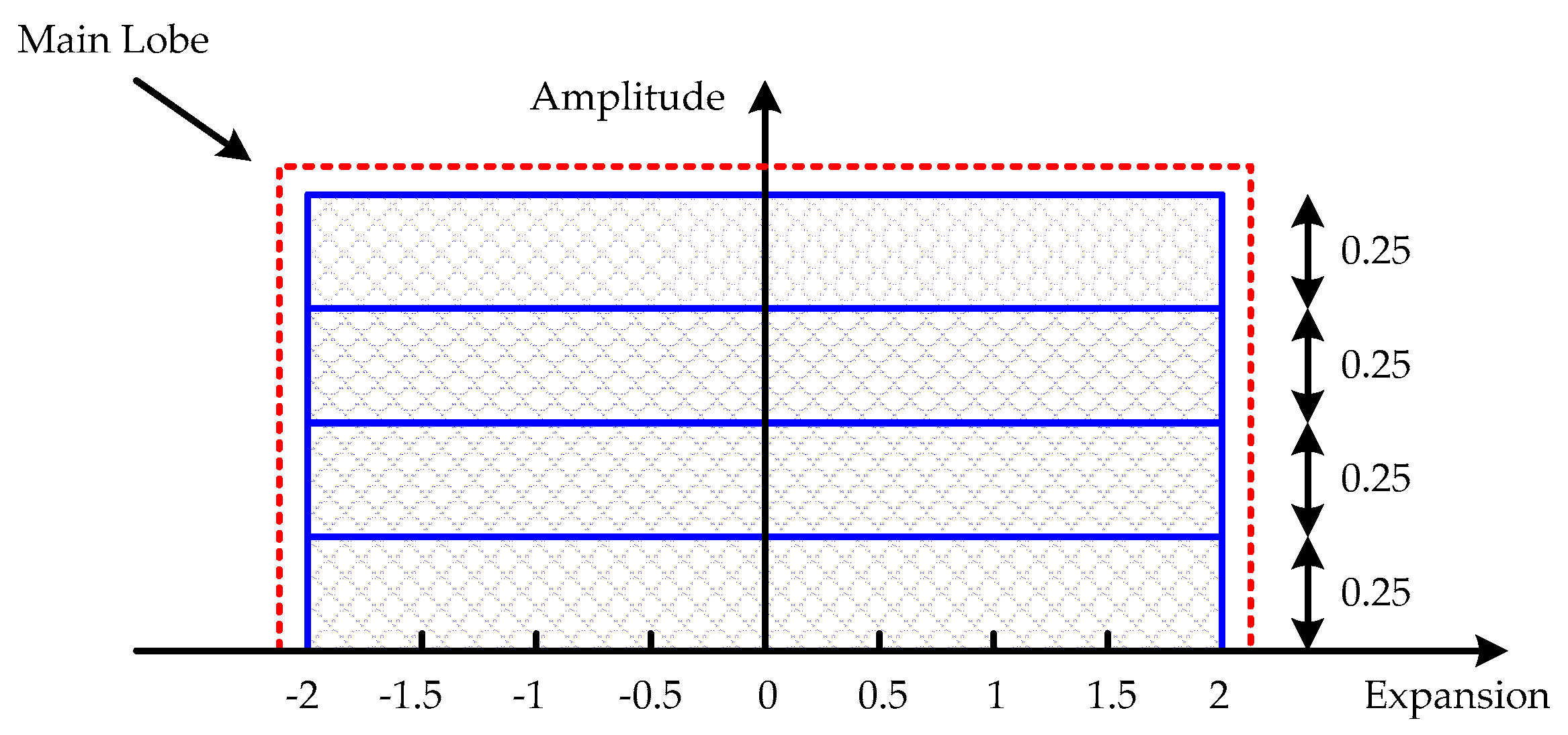
Though there is a difference between $s_{MPSM}\left(t\right)$ with the even number of sections $p$ and the odd number of sections $p$, the $\sin c$ function in $s_{MPSM}\left(t\right)$ with the even number of sections $p$ and the $\sin c$ function in $s_{MPSM}\left(t\right)$ with the odd number of sections $p$ are the same, which means the $\sin c$ function is only determined by the number of sections $p$, whether it is even or odd. According to the analysis above, the main lobe width of $s_{MPSM}\left(t\right)$ is $p$ times that without MPSM, which means the effective jamming range of MPSM jamming is $p$ times that of the original signal according to the number of sections $p$. When the section length $\left(a_{i+1}-a_i\right)$ is equal, for example, each section length is equal, and each section length is 0.25 of the pulse width $T$, the envelope result of the summation of four sections is simplified in Figure 3.

In Equations (11) and (12), the summation term $\sum$, which determines the waveform and value in the main lobe, is only determined by the modulation phase ${\varphi }_i$ when the number of sections $p$ is a fixed value. The influence of the modulation phase ${\varphi }_i$ will be analyzed in Section 3.2.

3.1.2. Random Section Length

When the section situation has a random section length, $s_{MPSM}\left(t\right)$ can only be simplified using Equation (12) due to the different lengths of each section.

$$s_{MPSM}\left(t\right)=\exp \left(-j\pi K{t}^2\right)\times {\displaystyle \sum _{i=1}^p\exp \left(j{\varphi }_i\right)\times \exp \left(j\pi Kt\left(a_i+a_{i+1}\right)\right)\times \left(a_{i+1}-a_i\right)\times \sin c\left(Kt\left(a_{i+1}-a_i\right)\right)}$$

(13)

In Equation (13), the envelope determined by the $\sin c$ function of each term in the summation $\sum$ is all different because the section length $\left(a_{i+1}-a_i\right)$ is all different. Thus, the main lobe width of $s_{MPSM}\left(t\right)$ is hard to calculate according to the section situation with random section lengths.

Equation (13) shows that for longer section lengths $\left(a_{i+1}-a_i\right)$, the main lobe width of the $\sin c$ function expands less, but the amplitude coefficient $\left(a_{i+1}-a_i\right)$ is larger, which means the power of the section is larger. For shorter section lengths $\left(a_{i+1}-a_i\right)$, the main lobe width of the $\sin c$ function expands more, but the amplitude coefficient $\left(a_{i+1}-a_i\right)$ is smaller, which means the power of the section is smaller. Thus, the expansion of the main lobe width of $s_{MPSM}\left(t\right)$ cannot be accurately obtained when the section length $\left(a_{i+1}-a_i\right)$ is random.

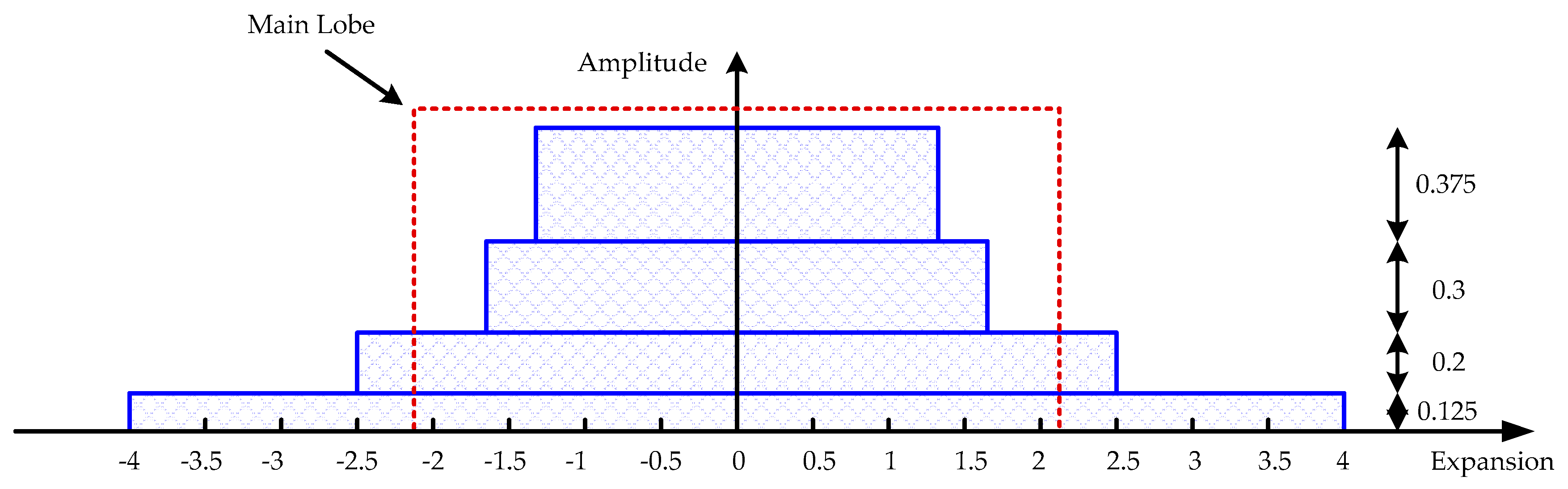
However, when the section length $\left(a_{i+1}-a_i\right)$ is random, for example, 0.125, 0.2, 0.3, and 0.375, the envelope result of the summation of four sections is shown in Figure 4. The red dotted line is the same as that in Figure 5. In Figure 5, when the number of sections is a fixed value, the main lobe with a random section length can be approximated as the main lobe of equal section length. The greater the number of sections, the higher the accuracy of approximation.

Therefore, when the number of sections is $p$, for unity and convenient application of two kinds of section situations, the main lobe width of $s_{MPSM}\left(t\right)$ is set to $p$ times that of the main lobe width of the signal without MPSM.

3.2. Phase Situation

Equation (10), which can be expressed as Equation (14), shows that the phase situation ${\varphi }_i$ mainly affects the phase of items in $\sum$.

$$s_{MPSM}\left(t\right)=\exp \left(-j\pi K{t}^2\right)\times {\displaystyle \sum _{i=1}^p\exp \left(j{\varphi }_i\right)\times \left\{\exp \left(j\pi Kt\left(a_i+a_{i+1}\right)\right)\times \left(a_{i+1}-a_i\right)\times \sin c\left(Kt\left(a_{i+1}-a_i\right)\right)\right\}}$$

(14)

When section situation has equal section lengths, Equation (14) can be simplified as Equation (15), where $A\left(t\right)=\exp \left(-j\pi K{t}^2\right)\times \left(a_{i+1}-a_i\right)\times \sin c\left(Kt\left(a_{i+1}-a_i\right)\right)$ and $\exp \left(j{\phi }_i\right)=\exp \left(j{\varphi }_i\right)\times \exp \left[j\pi Kt\left(a_i+a_{i+1}\right)\right]$.

$$s_{MPSM}\left(t\right)=A\left(t\right)\times {\displaystyle \sum _{i=1}^p\exp \left(j{\phi }_i\right)}$$

(15)

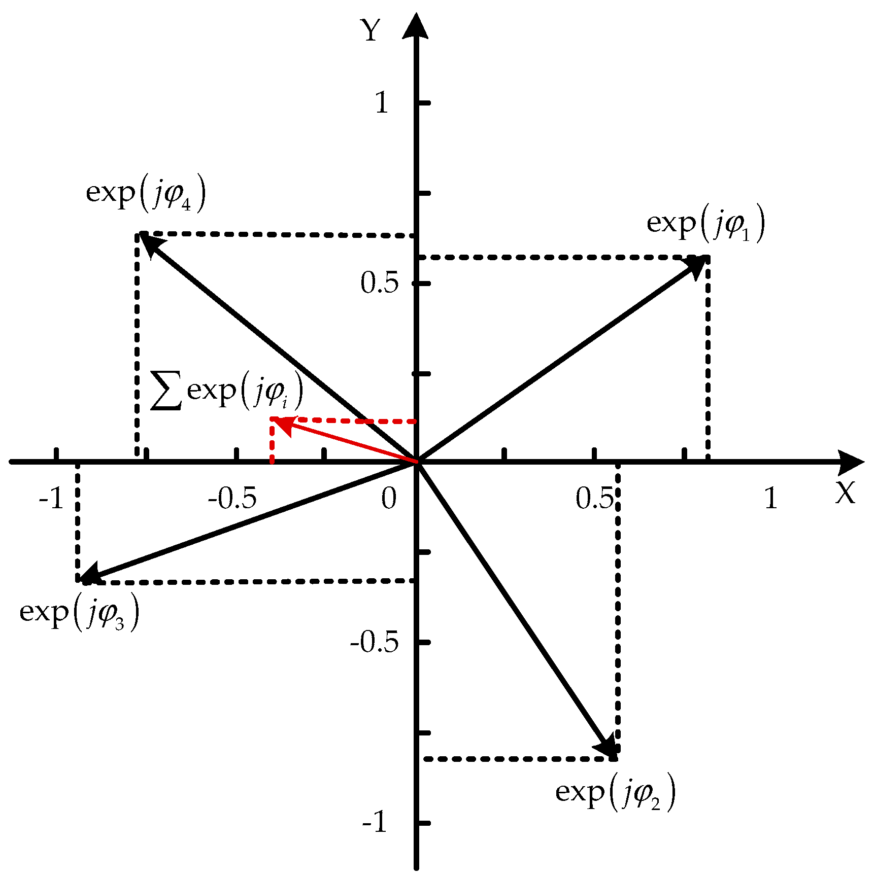
The phase situation ${\varphi }_i$ mainly affects the calculation results of the $\sum$ term, which is the jamming waveform within the main lobe width of $s_{MPSM}\left(t\right)$. When the phase situation ${\varphi }_i$ is random, the calculation results of the $\sum$ term will be complex due to the summation of the random vectors, and the amplitude of the $\sum$ term may be decreased when the phase situation ${\varphi }_i$ is under some situations, which is shown in Figure 5.

In Figure 5, it is difficult to find the corresponding relationship between the results and parameter setting of MPSM jamming.

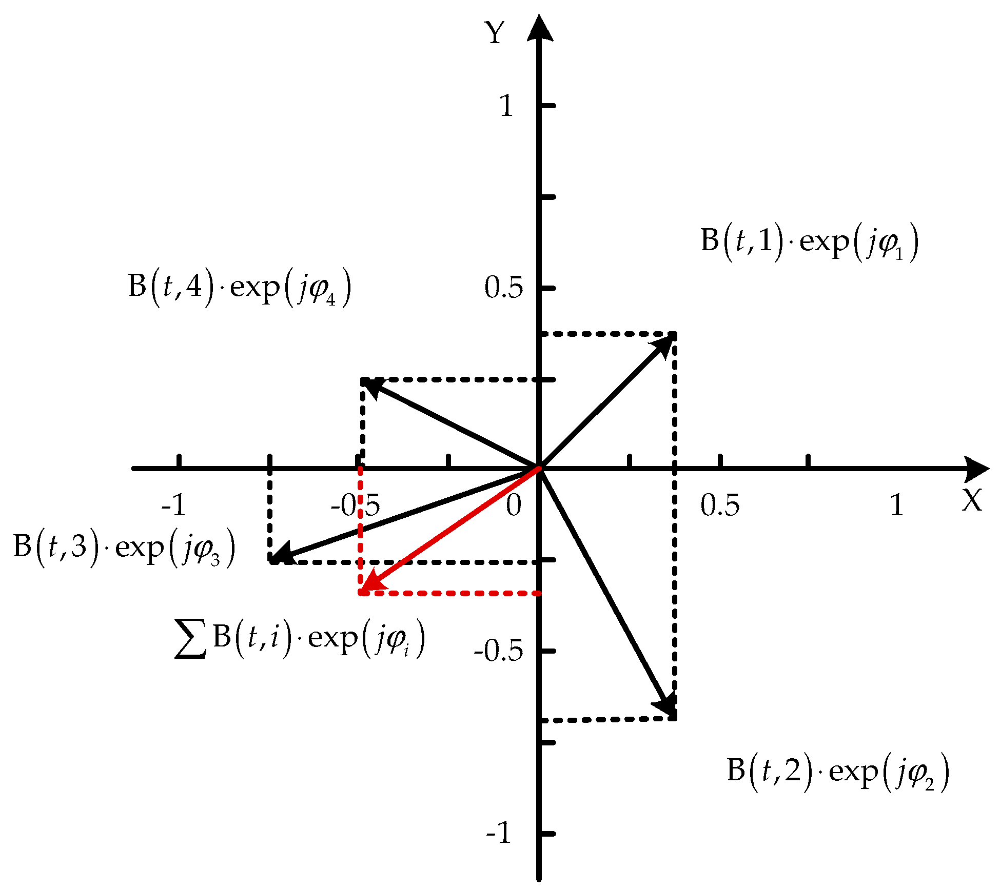
When the section length is random, Equation (14) can be simplified as Equation (16), where $\mathrm{B}\left(t,i\right)=\exp \left(-j\pi K{t}^2\right)\times \left(a_{i+1}-a_i\right)\times \sin c\left[Kt\left(a_{i+1}-a_i\right)\right]$ and $\exp \left(j{\phi }_i\right)=\exp \left(j{\varphi }_i\right)\times \exp \left(j\pi Kt\left(a_i+a_{i+1}\right)\right)$. The calculation difficulty of the $\sum$ term is further complicated because of the random section length.

$$s_{MPSM}\left(t\right)={\displaystyle \sum _{i=1}^p\mathrm{B}\left(t,i\right)\times \exp \left(j{\phi }_i\right)}$$

(16)

When the phase situation ${\varphi }_i$ and section situation $\left(a_{i+1}-a_i\right)$ are random, the calculation results of the $\sum$ term will be more complex due to the summation of random vectors whose amplitudes are modulated by $\mathrm{B}\left(t,i\right)$ related to the section length $\left(a_{i+1}-a_i\right)$. The amplitude of the $\sum$ term may decrease when the phase situation ${\varphi }_i$ is under some situations, as shown in Figure 6.

In Figure 6, the corresponding relationship between the results and parameter setting of MPSM jamming is harder to obtain. Therefore, it is necessary to use another method to obtain the optimal local suppression jamming effect and its corresponding parameter settings.

4. Optimization Algorithm for MPSM Jamming

Particle swarm optimization (PSO) is an intelligent optimization algorithm proposed by Kennedy and Eberhart in 1995 [25,26]. The algorithm simulates the foraging behavior of a bird group and promotes the whole bird group to find the food source through cooperation among the birds [27,28]. The purpose of this meta-heuristic technique is to solve complex global optimization problems. Compared with other meta-heuristic algorithms, such as genetic algorithms (GAs), PSO has advantages, such as less steps of algorithm, less memory usage, shorter computation time, faster convergence speed and higher precision. PSO has attracted the attention of academia for its advantages [29]. Therefore, this paper chooses PSO to solve the problem.

Unlike traditional GAs [30], PSO does not require traditional population evolution, crossover, or mutation operations, but uses a new mechanism: information transfer, swarm intelligence, and population topology. Similar to GAs, PSO has a fitness function value, which is updated by iteration. The main difference between GA and PSO is that each particle in PSO benefits from its previous motion, whereas each individual in GA benefits from crossover and mutation operations, which makes PSO simpler in operation. In PSO, the particles follow the optimal particle to search the optimal solution. This process is like the predation of a group of birds, which randomly searches for the only food in an area. Not all birds know where the food is, but they know how far they are from the food. The simplest and most effective method is to search around the area nearest to the food, which is the source of the PSO. PSO relies on collective wisdom. Each particle adjusts its position and speed according to the best solution obtained by the whole particle swarm and the best solution found separately. Because of its high efficiency, PSO is widely used in acoustics [31], electronics [32], reverse engineering [29], and other fields [33,34].

4.1. Principle of PSO Algorithm

For a certain number of particles, each particle represents a potential solution to the problem. When population number is m, PSO algorithm involves the process of searching for the optimal particle in the search space of N dimension solutions.

$$X_i={\left(x_{i1},x_{i2},\dots ,x_{iN}\right)}^T,V_i={\left(v_{i1},v_{i2},\dots ,v_{iN}\right)}^T$$

(17)

$$fitnes{s}_i=F\left(X_i\right),\left(i=1,2,\dots ,m\right)$$

(18)

Equation (17) defines the position vector and velocity vector of the $i\mathrm{th}$ particle in $N$ dimension. In Equation (18), $F\left(X_i\right)$ is the fitness function of the particle, and $fitness$ is the corresponding fitness value of the particle. In a PSO algorithm, all particle optimization processes in the population adjust their velocity and position according to the following equations:

$$v_{id}^{k+1}=w\times v_{id}^k+c_1{r}_1\left(x_{id}^{Pbest}-x_{id}^k\right)+c_2{r}_2\left(x_d^{gbest}-x_{id}^k\right),\left(k=1,2,\dots ,\max gen\right)$$

(19)

$$x_{id}^{k+1}=x_{id}^k+v_{id}^{k+1}$$

(20)

$$Pbes{t}_i,X_{id}^{Pbest},gbest,X_d^{gbest},\left(d=1,2,\dots ,N\right)$$

(21)

Equation (19) is the velocity adjustment equation of PSO. On the right side of the equation, the first term is the initial velocity of the particles, the second term is the cognitive term of the particles, which reflects the cognitive ability of the particles themselves, and the last term is the social term of the particles, which reflects the ability to transmit information and cooperation between particles. $v_{id}$ and $x_{id}$ are the d-dimensional components of the velocity and position of particle $i$, respectively; $k$ is the number of iterations; $\max gen$ is the maximum number of iterations, $w$ is the inertial weight; $r_1$ and $r_2$ are random numbers between 0 and 1; and $c_1$ and $c_2$ are the acceleration coefficients. Equation (20) is the particle position adjustment PSO equation, in which the first item on the right side of the equation is the initial position of particle $i$ and the second item is the updated velocity.

The position adjustment of PSO depends on a particle’s own experience and the experience of its neighbors. The velocity vector is the driving force of the whole optimization process that reflects the experience of the particle itself and the social interaction information of its neighbors. In Equation (21), $Pbes{t}_i$ is the best fitness value of particle $i$, $X_{id}^{Pbest}$ is the position vector corresponding to the best fitness value of particle $i$, $gbest$ is the best fitness value of all particles in the solution group, and $X_d^{gbest}$ is the position vector corresponding to the best fitness value of all particles in the solution group.

In PSO, the balance between the global and local exploration abilities is mainly controlled by the inertia weight. PSO with an appropriate inertia weight was found to perform better with a greater chance of finding the global optimal solution within a reasonable number of iterations [35].

4.2. Analysis of Parameters in PSO

4.2.1. Inertia Weight

Inertial weight $w$ denotes the influence by the results of the previous iteration. The larger the $w$, the greater the influence of the previous iteration. A larger $w$ helps obtain the global optimal solution, and a smaller $w$ helps to obtain the local optimal solution. Therefore, an appropriate $w$ can balance the global search ability and the local search ability, which can also balance the convergence speed and accuracy of the algorithm.

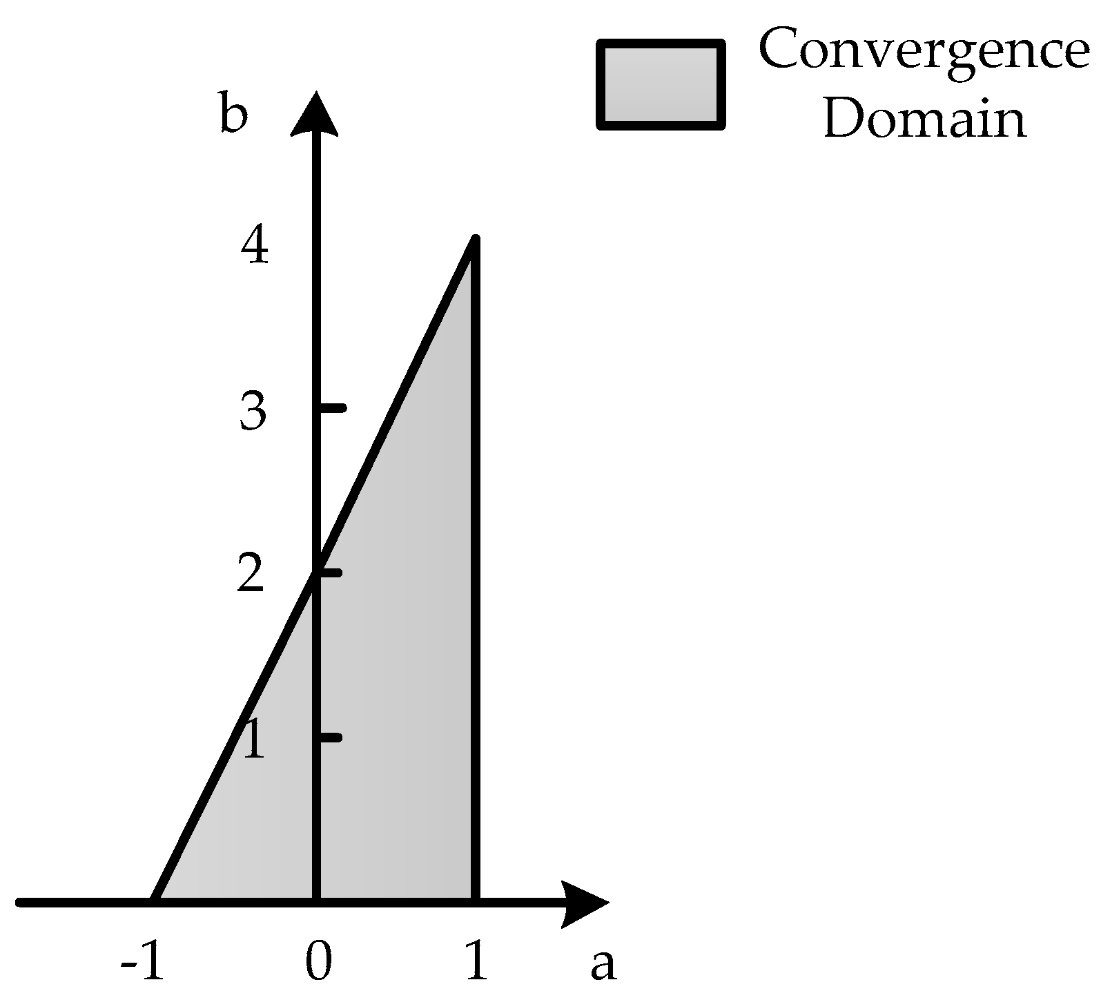
According to Trelea I C. [36], when $a<1$, $b>0$, $2a-b+2>0$, the PSO will converge, where $a=w$ and $b=\left(c_1+c_2\right)/2$. The convergence domain is shown in Figure 7.

For any initial position and velocity, the particle will converge to the global optimal result only if the algorithm parameters are selected inside this triangle. $w$ is set to 0.5 in this paper.

4.2.2. Acceleration Coefficient

Acceleration coefficients $c_1$ and $c_2$ reflect the information exchange in the population, which adjust the maximum step size of “flight” to the global optimal solution and individual optimal solution direction. $c_1$ and $c_2$ can accelerate the convergence and avoid falling into local optimal solution easily. When $c_1$ is small, the particle is influenced more by the individual experience, which means the algorithm converges faster, but falls into local optimal solutions easier. When $c_2$ is small, the particle is influenced more by the group experience, which means the algorithm struggles to obtain the optimal solution due to lacking information exchange. In general, $c_1$ and $c_2$ are set to be equal, which means an equivalent influence of individual experience and group experience and a higher efficiency. $c_1$ and $c_2$ were set to 2 in this paper.

4.2.3. Population Size

The larger the population size, the stronger the diversity of the population, and the greater the probability of obtaining the global optimal solution. However, the increase in population size increases the computation requirements.

4.3. Analysis of Fitness Function and Fitness Value

It is necessary to set an appropriate fitness function and fitness value to represent the optimization effect by the PSO algorithm. The aim of the optimization of MPSM jamming is to find the optimal local suppression jamming effect and corresponding parameter settings in the combination of many section situations and phase situations. The optimal local suppression jamming effect can suppress the target or key area, destroy the target characteristics information, and even completely cover the target. To evaluate the jamming effect of local suppression jamming, the suppression range and the energy distribution in the range should be considered.

According to the previous analysis, when the number of sections is $p$, the expansion of the main lobe width of MPSM jamming is set to $p$ times the main lobe width of the signal without MPSM. According to the principle and property of pulse compression of an LFM signal, the more serious the signal mismatch, the lower the peak value after pulse compression, and the stronger the expansion of the main lobe width. For MPSM jamming, the lower the peak value of the main lobe, the greater the expansion of the main lobe, the more uniform the jamming energy distribution in main lobe, and the higher the mean value of the main lobe, which means a better local suppression jamming effect.

Based on this, the effect of local suppression jamming can be characterized by the amplitude of peak value of MPSM jamming: the lower the peak value, the better the effect of local suppression jamming; the higher the peak value, the worse the effect of local suppression jamming. Therefore, when number of sections is $p$, the fitness value of PSO is set as the peak value in the main lobe of $s_{MPSM}\left(t\right)$.

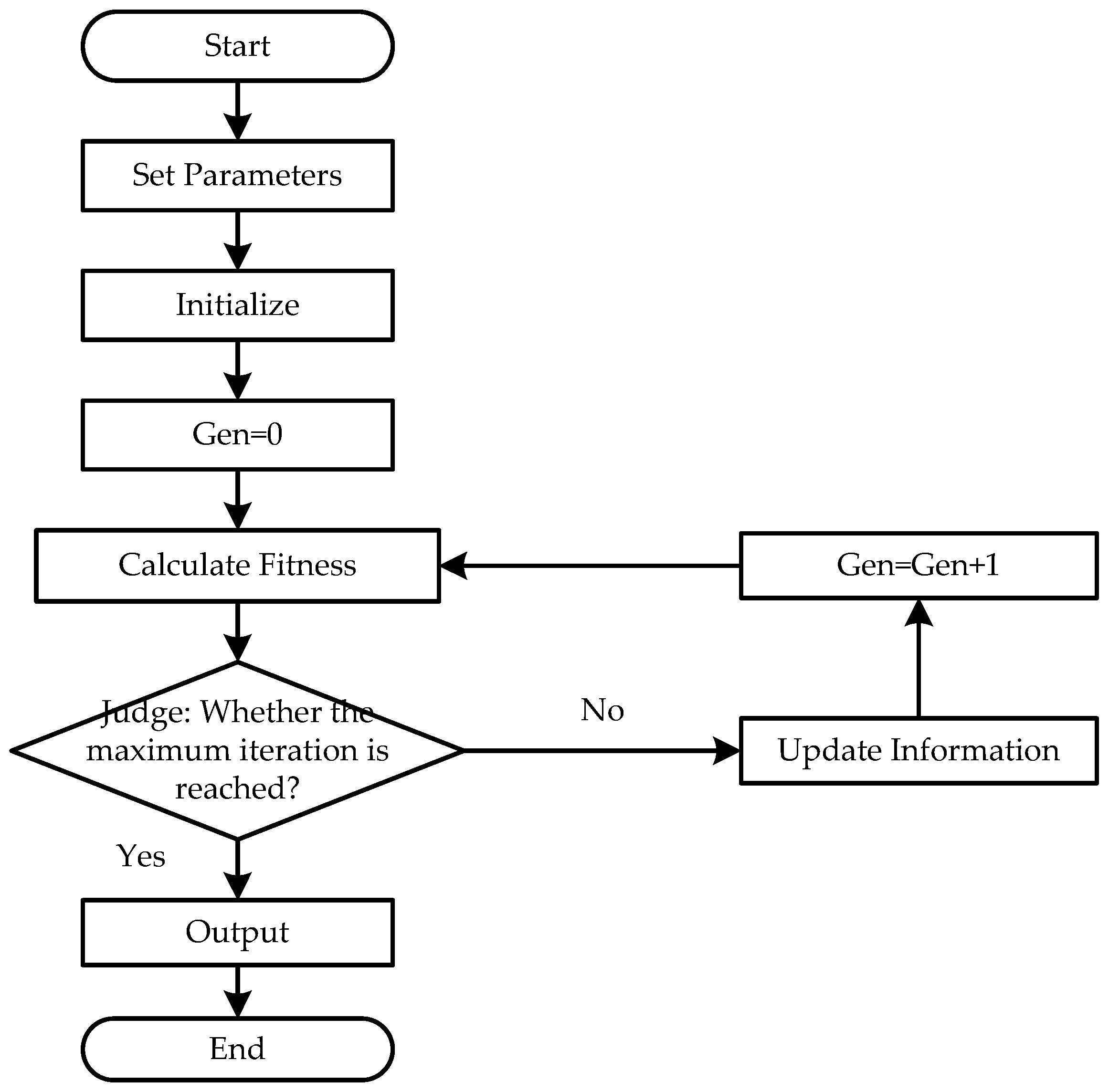
4.4. Steps of Optimization Algorithm for MPSM Jamming Based on PSO

According to the principle of PSO and the optimization analysis of the fitness function and fitness value, the steps of the optimization algorithm for MPSM jamming based on PSO are shown in Figure 8.

Step 1: Determine the search dimension $N$, population size $m$, maximum iterations maxgen, and acceleration coefficients $c_1$ and $c_2$. According to the different optimization objects, the search dimension is also different. For $p$-section MPSM jamming, the dimension is $p$ when the phase situation is optimized, $p$ when the section situation is optimized, and $2p$ when the section and phase situation are optimized. For specific or complex optimization problems, the population size $m$ can be set between 50 and 200, and the population size in this paper was set to 100. The maximum iterations $\max gen$ reflect the evolutionary efficiency of the algorithm; too large a $\max gen$ will cause waste calculation time, and too small a $\max gen$ may not achieve the optimization goal. The maximum number of iterations $\max gen$ in this paper was set to 1000. $c_1$ and $c_2$ are usually between 0 and 4. In this paper, $c_1$ and $c_2$ were set to 2.

Step 2: Initial position value $x_{id}$ and speed value $v_{id}$.

Step 3: Calculate the fitness value $fitness$ of each particle, the best fitness value $Pbes{t}_i$ of each individual, the best fitness value $gbest$ of the population, the best position value $X_{id}^{Pbest}$ of each individual, and the best position value $X_d^{gbest}$ of the population. According to the previous analysis, the particle fitness value is the peak value in the main lobe of $s_{MPSM}\left(t\right)$.

Step 4: Judge whether the maximum iteration is reached. If so, go to Step 6, otherwise continue.

Step 5: Update speed and location and return to Step3.

Step 6: End the algorithm and output the results.

5. Experiments and Results

5.1. Parameter Settings

Some of simulation parameter settings are shown in

Table 1. Parameter settings.

Parameter	Value	Unit
bandwidth	100	Hz
pulse width	1	s
frequency rate	100	Hz/s
sampling rate	2000	Hz
sampling points	2000
Jamming-signal power ratio (JSR)	0	dB

.

5.2. Comparison of Convergence and Computation Time with Different PSO Parameters

5.2.1. Inertia Weight

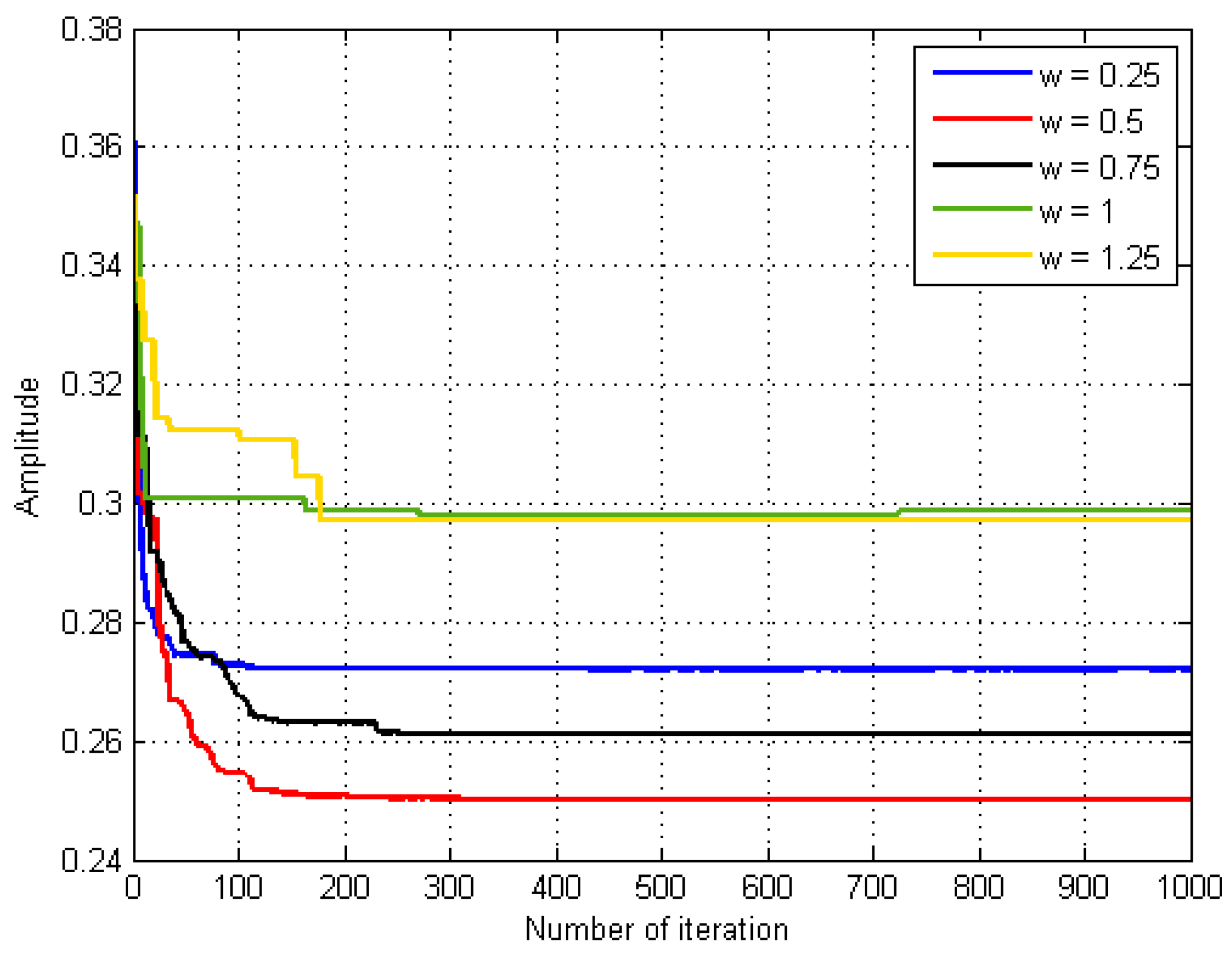
The purpose of this simulation was to compare the convergence and computation time with different inertia weights. We chose different inertia weights: 0.25, 0.5, 0.75, 1, and 1.25. The results of convergence are shown in Figure 9, and the results of computation time are shown in

Table 2. Computation time with different inertia weights.

Inertia Weight	Computation Time (s)
0.25	123
0.5	109
0.75	107
1	130
1.25	132

.

In Figure 9, when the inertia weight was 0.5, the convergence effect was the best. In Table 2, when the inertia weight was 0.5, the computation time was almost the same as that of 0.75, which is the shortest computation time. So, when the inertia weight is 0.5, the global search ability and the local search ability, as well as the convergence speed and accuracy of the algorithm, are best balanced.

5.2.2. Acceleration Coefficient

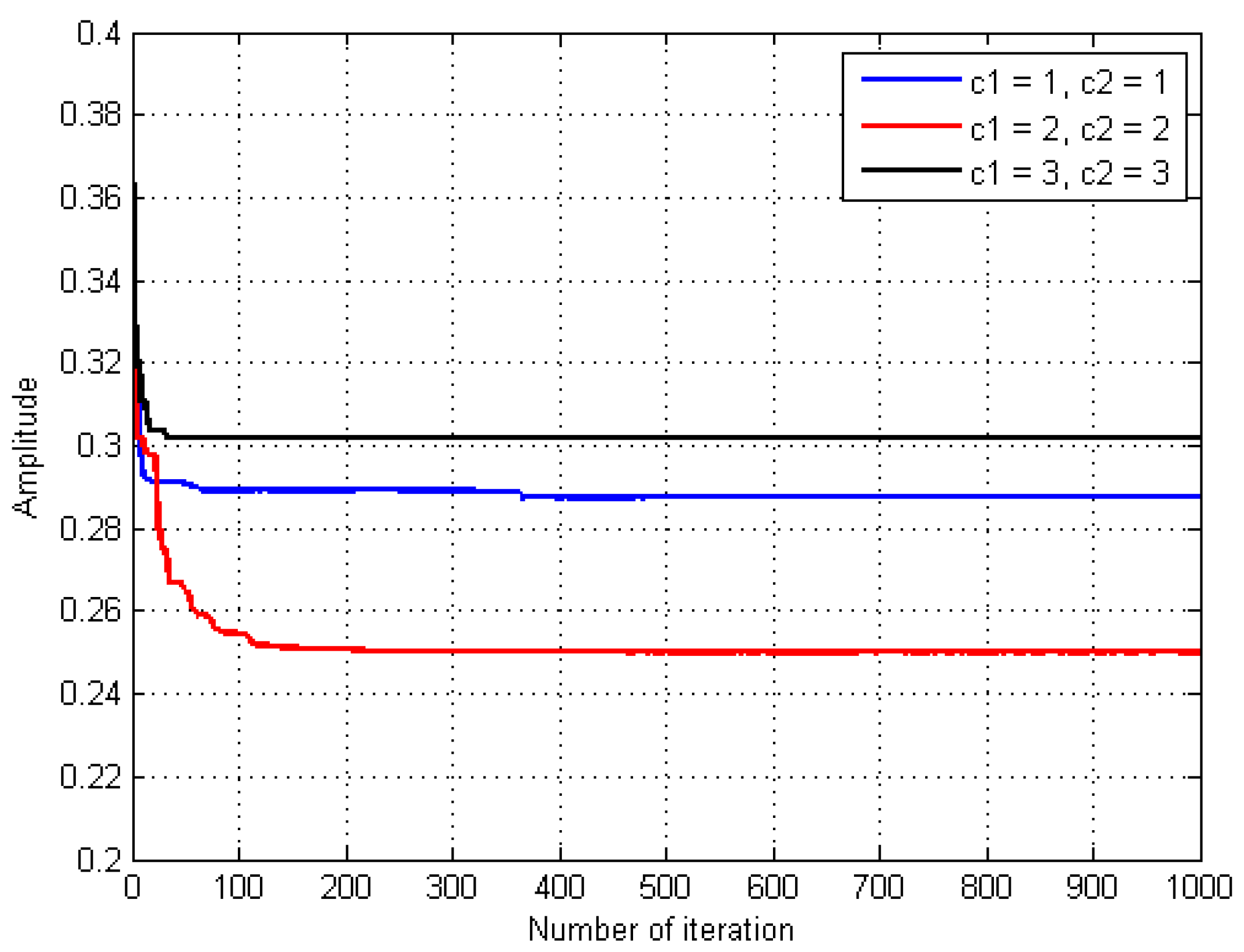
The purpose of this simulation was to compare the convergence and computation time with different acceleration coefficients. We chose different acceleration coefficients: 1, 2, and 3. The results of convergence are shown in Figure 10, and the results of computation time are shown in

Table 3. Computation time with different acceleration coefficients.

Acceleration Coefficient	Computation Time (s)
1	116
2	109
3	133

.

In Figure 10, when the acceleration coefficient was 2, the convergence effect was the best. In Table 3, when the acceleration coefficient was 2, the computation time was the shortest. So, when the acceleration coefficient is 2, the global search ability and the local search ability, as well as the convergence speed and accuracy of the algorithm are best balanced.

5.2.3. Population Size

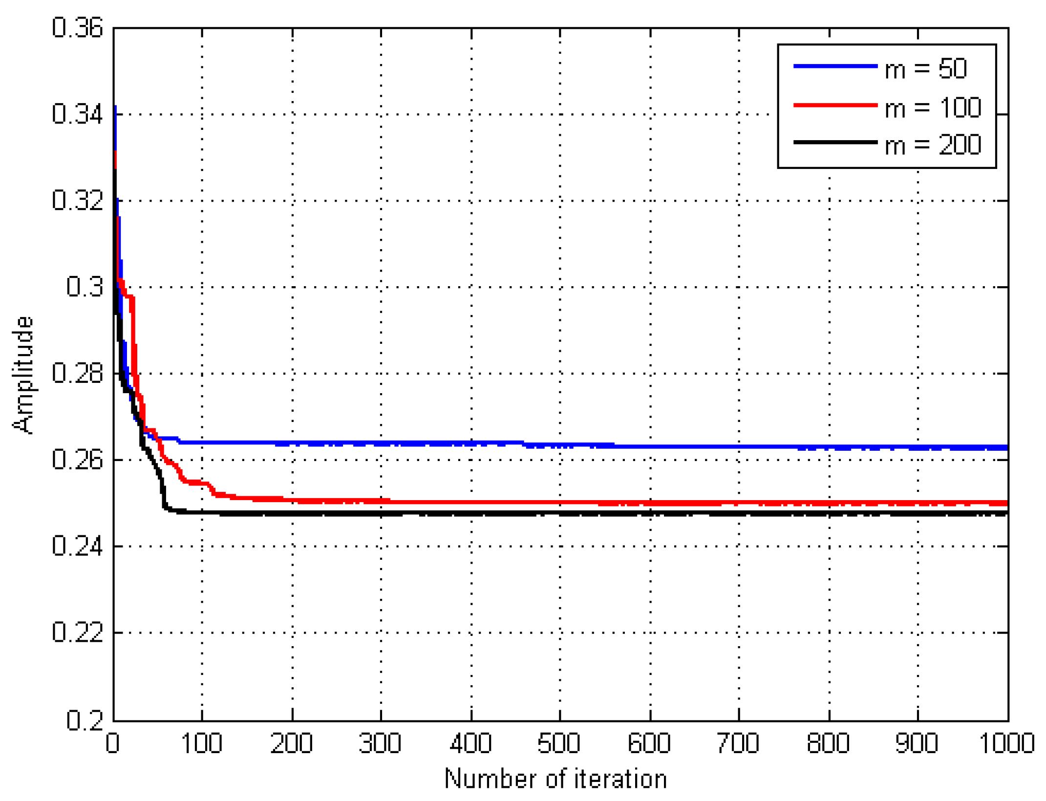
The purpose of this simulation was to compare the convergence and computation time with different population sizes. We chose different population sizes: 50, 100, and 200. The results of convergence are shown in Figure 11, and the results of computation time are shown in

Table 4. Computation time with different population sizes.

Population Size	Computation Time (s)
50	81
100	109
200	324

.

In Figure 11, when the population size was 200, the convergence effect was the best. In Table 4, when the population size was 50, the computation time was the shortest. To balance the convergence speed and accuracy, when the population size is 100, the convergence speed and accuracy of the algorithm are best balanced.

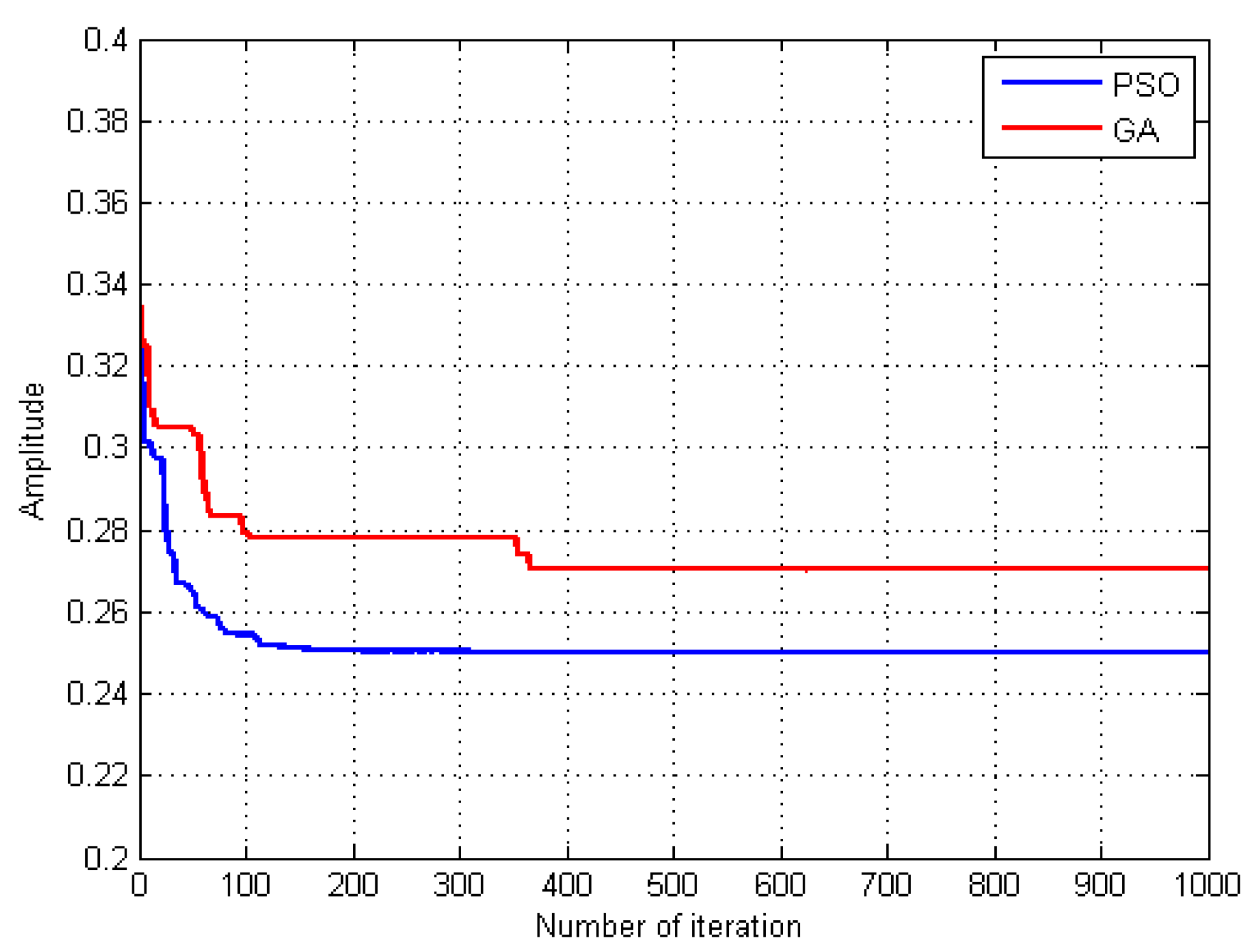
5.3. Comparison of Convergence and Computation Time of PSO and GA

The purpose of this simulation was to compare the convergence and computation time between PSO and GA. For comparison, the parameters of GAs are set as follows: chromosome is coded in decimal system, population size $m$ is set to be 100, iteration number $N$ is set to be 1000, crossover rate is set to be 1 which means crossover happens every iteration, mutation rate is set to be 0.1. The results of convergence are shown in Figure 12, and the results of computation time are shown in

Table 5. Computation time of PSO and GA.

Algorithm	Computation Time (s)
PSO	109
GA	354

.

In Figure 12, PSO produced a better convergence effect. In Table 5, PSO required less computation time. According to the analysis and simulation, PSO converges faster, and requires less computation time.

5.4. Relationship Between Number of Sections and Main Lobe Width

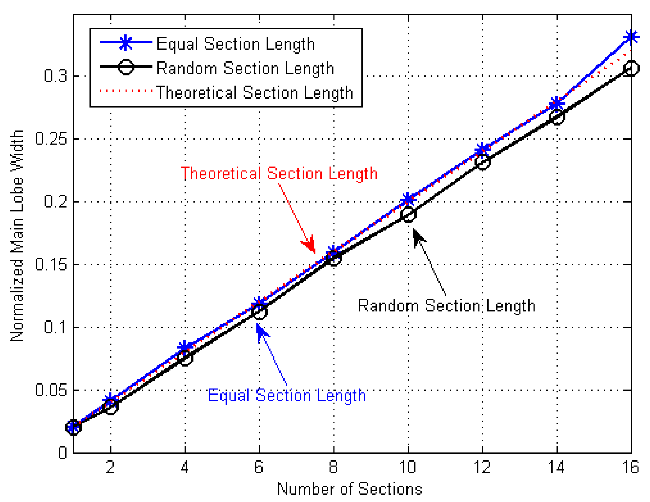
The purpose of this simulation was to verify the relationship between the number of sections and the main lobe width of MPSM jamming, which contributes to calculating the evaluation factors and quantitatively comparing the MPSM jamming effect. According to the analysis above, the main lobe width of MPSM jamming was set to $p$ times that of the original signal after pulse compression. According to the parameter settings in Section 5.1, the normalized main lobe width is 0.02. Therefore, the theoretical value of the normalized main lobe width of MPSM jamming is $0.02\times p$, where $p$ is the number of sections, as shown in Figure 13 as the red dotted curve.

Taking as examples the MPSM jamming with the section situation of equal section lengths and random section length, the simulation completed 100 Monte Carlo experiments for different numbers of sections. When the section situation is equal section lengths, the main lobe width of MPSM jamming is calculated by finding the zero positions on both sides of the peak value, then counting and averaging, which is shown in Figure 13 as the blue curve with Asterix marks. When the section situation is random section lengths, the main lobe width of MPSM jamming is calculated by finding the side lobes on both sides of the main lobe, then counting and averaging, which is shown in Figure 13 as the black curve with circle marks.

In Figure 13, the main lobe width of MPSM jamming with equal section length increases with the number of sections, whose curve is in good agreement with the curve of the theoretical results, which proves the correctness of the theoretical derivation in Section 3.1.1. The main lobe width of MPSM jamming with random section lengths also increases with the number of sections, and the value of the random section length is slightly lower than the curve of the theoretical results. According to the analysis and simulation results, it is feasible and acceptable to set the main lobe width of the p-sections MPSM jamming as p times that of the original signal after pulse compression, whether the section situation is equal or random section lengths.

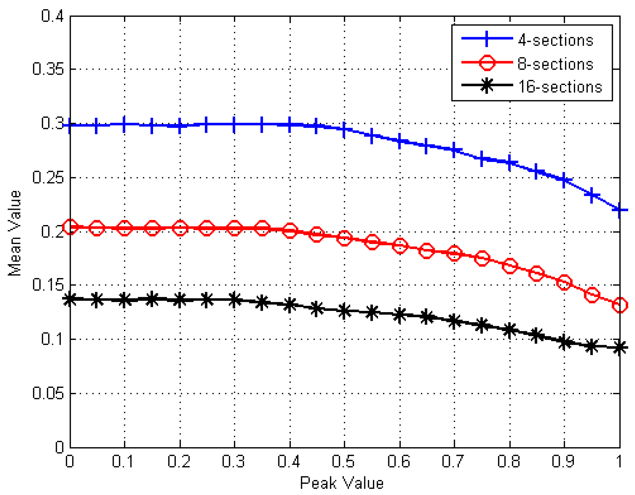
5.5. Relationship Between Peak Value and Mean Value of Main Lobe

The purpose of this simulation was to verify the relationship between the peak value and the mean value of the main lobe of MPSM jamming, which contributes to the correctness of the fitness function and fitness value in Section 4.3. Taking 4, 8, and 16 sections MPSM jamming as examples, the simulation completed 1000 Monte Carlo simulation experiments. The mean value of the main lobe was used to characterize the jamming power within main lobe width.

By calculating the peak value and the corresponding mean value of the main lobe, the results were fitted and are shown in Figure 14. The blue curve with cross marks is the result of four sections of MPSM jamming, the red curve with circle marks is the result of eight sections of MPSM jamming, and the black curve with rice marks is the result of 16 sections of MSPM jamming.

As shown in Figure 14, the mean value of the main lobe decreases with the peak value, which means that there is a negative correlation between them. The lower the mean value of the main lobe, the more uneven the jamming power distribution within the main lobe. Therefore, the simulation results show that the peak value is negatively correlated with the uniformity of energy distribution, which means that the lower the peak value, the more uniform the jamming power distribution. In Figure 14, the mean value of the main lobe is greater when the number of sections is greater because the number of sections is greater. The expansion range of the jamming power is greater, which is consistent with the theoretical derivation and the simulation results. According to the analysis and simulation results, it is feasible and acceptable to set the fitness value as the peak value to characterize the distribution of jamming power for certain sections.

5.6. Random MPSM Jamming and Optimized MPSM Jamming

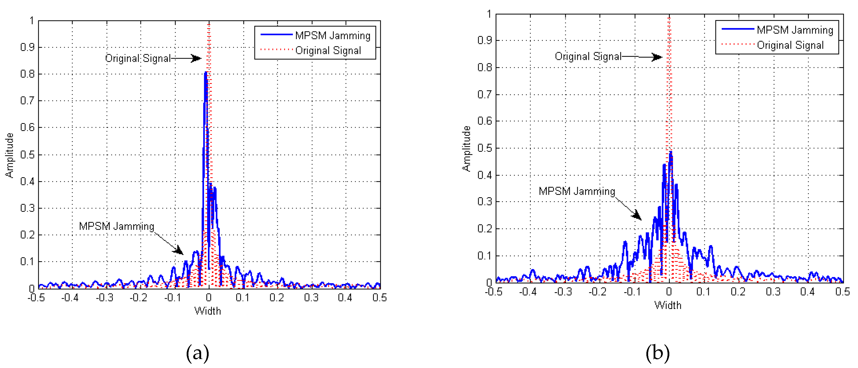
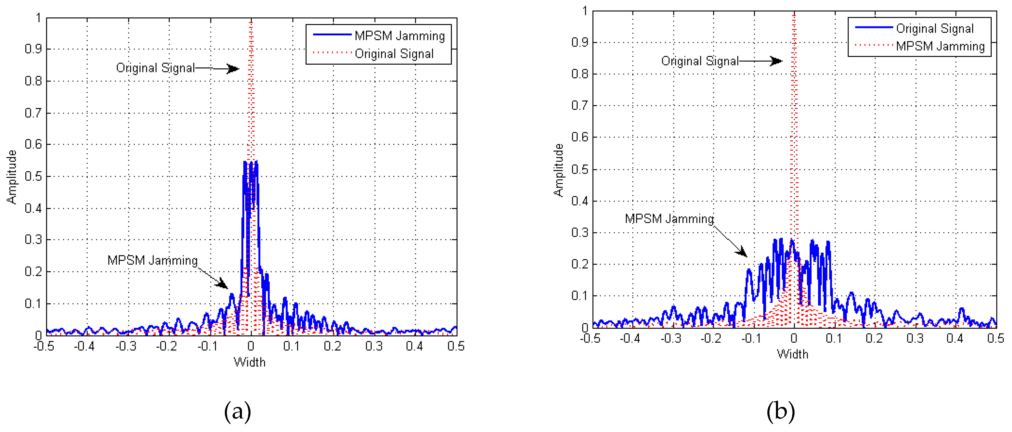
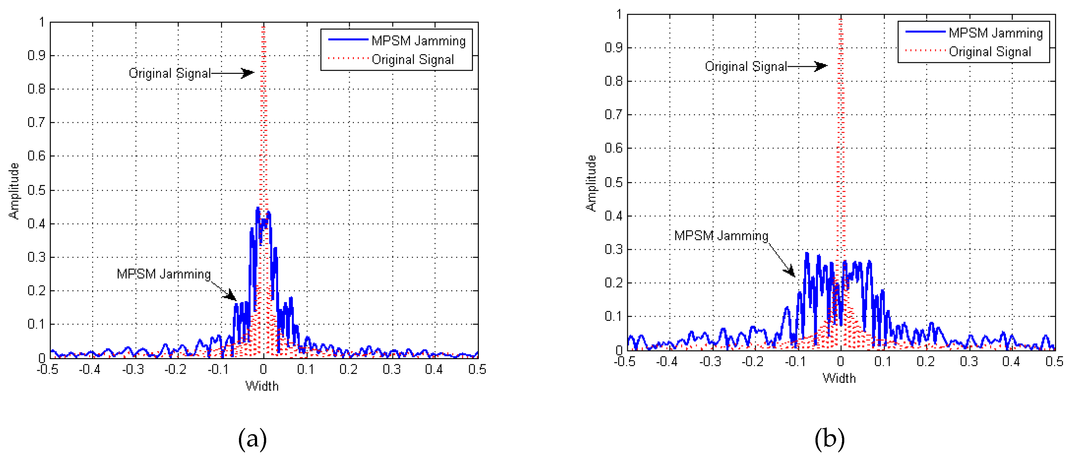
The purpose of simulation in this section was to verify the effectiveness of MPSM jamming and the effectiveness of the MPSM optimization algorithm jamming based on PSO. Taking 4 sections and 16 sections of MPSM jamming as examples, we simulated the results of MPSM jamming under a random section situation and phase situation. The results of MPSM jamming for the optimized section situation, the results of MPSM jamming for the optimized phase situation, and the results of MPSM jamming for the optimized section situation and phase situation are shown in Figure 15, Figure 16, Figure 17 and Figure 18 and

Table 6. Parameter settings of MPSM jamming with random sections and phase situation.

Figure 15	Section Situation	Phase Situation
(a)	0.250, 0.315, 0.410, 0.025	0.095π, 0.685π, 1.472π, 1.589π
(b)	0.025, 0.082, 0.057, 0.112, 0.042, 0.041, 0.061, 0.061, 0.055, 0.124, 0.058, 0.039, 0.080, 0.001, 0.092, 0.070	1.107π, 1.454π, 1.970π, 0.525π, 0.315π, 0.723π, 0.227π, 0.360π, 1.127π, 0.677π, 0.379π, 1.506π, 0.205π, 1.588π, 0.021π, 0.020π

,

Table 7. Results of MPSM jamming in Figure 15.

Figure 15	Peak	Mean	Entropy
(a)	0.810	0.264	0.726
(b)	0.487	0.137	0.905

,

Table 8. Parameter settings of MPSM jamming with optimized section situation.

Figure 16	Section Situation	Phase Situation
(a)	0.114, 0.184, 0.079, 0.623	0.095π, 0.685π, 1.472π, 1.589π
(b)	0.083, 0.085, 0.046, 0.060, 0.068, 0.124, 0.045, 0.070, 0.116, 0.096, 0.097, 0.060, 0.017, 0.017, 0.008, 0.008	1.107π, 1.454π, 1.970π, 0.525π, 0.315π, 0.723π, 0.227π, 0.360π, 1.127π, 0.677π, 0.379π, 1.506π, 0.205π, 1.588π, 0.021π, 0.020π

,

Table 9. Results of MPSM jamming in Figure 16.

Figure 16	Peak	Mean	Entropy
(a)	0.591	0.282	0.727
(b)	0.357	0.138	0.923

,

Table 10. Parameter settings of MPSM jamming with optimized phase situation.

Figure 17	Section Situation	Phase Situation
(a)	0.114, 0.184, 0.079, 0.623	0.325π, 1.067π, 0.468π, 1.567π
(b)	0.083, 0.085, 0.046, 0.060, 0.068, 0.124, 0.045, 0.070, 0.116, 0.096, 0.097, 0.060, 0.017, 0.017, 0.008, 0.008	0.341π, 1.465π, 1.146π, 0.073π, 0.758π, 1.608π, 0.159π, 0.109π, 0.836π, 0.478π, 1.706π, 0.620π, 1.841π, 1.504π, 0.398π, 1.430π

,

Table 11. Results of MPSM jamming in Figure 17.

Figure 17	Peak	Mean	Entropy
(a)	0.549	0.275	0.805
(b)	0.281	0.141	0.939

,

Table 12. Parameter settings of MPSM jamming under optimized sections situation and the phase situation.

Figure 18	Section Situation	Phase Situation
(a)	0.154,0.242,0.151,0.453	0.751π,1.786π,0.794π,1.727π
(b)	0.106, 0.043, 0.058, 0.076, 0.069, 0.005, 0.018, 0.036, 0.138, 0.002, 0.095, 0.117, 0.071, 0.064, 0.049, 0.053	0.740π, 1.601π, 0.453π, 1.593π, 0.467π, 1.173π, 1.804π, 0.035π, 1.543π, 0.158π, 0.899π, 1.653π, 0.272π, 1.459π, 0.443π, 0.908π

and

Table 13. Results of MPSM jamming in Figure 18.

Figure 18	Peak	Mean	Entropy
(a)	0.429	0.300	0.798
(b)	0.290	0.133	1.028

. In the Figure 15, Figure 16, Figure 17 and Figure 18, the blue waveforms are the simulation results and the red dotted waveforms are the original signals after pulse compression.

5.6.1. Random Section Situation and Phase Situation

The parameter settings of MPSM jamming with random sections and the phase situation are shown in Table 6.

In Figure 15a,b, the main lobe of four sections of MPSM jamming expands less than four times. The main lobe of 16 sections of MPSM jamming expands less than 16 times. In Figure 15a,b, the waveforms are irregular within the main lobe width due to the random parameter settings, which means that the distributions of jamming power are non-uniform, making the jamming power concentrate in some peak values instead of uniformly in the main lobe, which decreases the local suppression jamming effect of MPSM jamming.

The entropy value of MPSM jamming is used to characterize the suppression jamming effect, which means that the greater the entropy value is, the better the suppression jamming effect is. By comparing the mean value and entropy value, what can be known is that the mean value and entropy value in Table 7 are less than that in Table 9, Table 11 and Table 13, which means that the local suppression jamming effect of MPSM jamming with random section situation and phase situation is worse than that with optimized parameter settings.

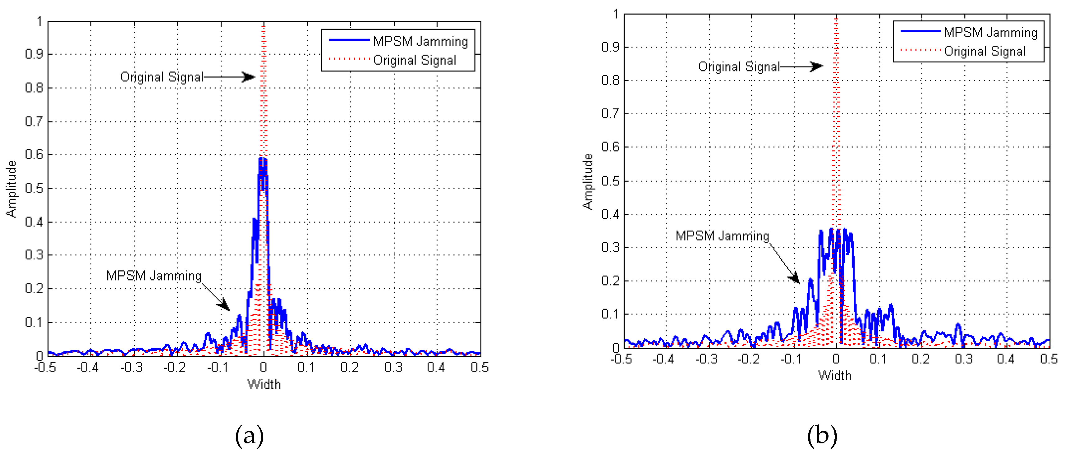
5.6.2. Optimized Section Situation

The parameter settings of MPSM jamming under the optimized section situation are shown in Table 8, where the phase situation is the same as that in Table 6.

In Figure 16a,b, the main lobe of four sections of MPSM jamming expands less than four times, the main lobe of 16 sections of MPSM jamming expands less than 16 times, and they are broader than those of MPSM jamming under the random sections situation and phase situation. There is a relatively plat part in the main lobe width of MPSM jamming with optimized section situation, where the jamming power is distributed uniformly. The flat part defined as the 3-dB width of MPSM jamming, is 0.02 for four sections and 0.08 for 16 sections, which are all 25% of the main lobe for four sections and 16 sections, respectively.

By comparing the peak value, mean value, and entropy value in Table 9 with those in Table 8, the mean value and entropy value of MPSM jamming with optimized section situation are shown to be greater than under the random sections situation and phase situation, which means that the local suppression jamming effect is better than under the random section situation and phase situation.

5.6.3. Optimized Phase Situation

The parameter settings of MPSM jamming with optimized phase situation are shown in Table 10.

In Figure 17a,b, the main lobe of four sections of MPSM jamming expands about four times, the main lobe of 16 sections of MPSM jamming expands about 16 times, and they are broader than those of MPSM jamming under the optimized section situation. There is a relatively flat part in the main lobe width of MPSM jamming under the optimized phase situation, where the jamming power is distributed uniformly. The flat part defined as the 3-dB width of MPSM jamming, is 0.036 for four sections and 0.156 for 16 sections, which are 45% and 48% of the main lobe, respectively.

By comparing the peak value, mean value, and entropy value of MPSM jamming in Table 11 and Table 7, the mean value and entropy value of MPSM jamming under the optimized phase situation are shown to be greater than MPSM jamming under the random section situation and phase situation, which means that the local suppression jamming effect of MPSM jamming under the optimized phase situation is better than under the random section situation and phase situation.

5.6.4. Optimized Section Situation and Phase Situation

The parameter settings for optimized sections and the optimized phase situation are shown in Table 12.

In Figure 18a,b, the main lobe of four sections of MPSM jamming expands about four times, the main lobe of 16 sections of MPSM jamming expands about 16 times, and they are broader than those of MPSM jamming under the optimized sections situation. There is a relatively flat part in the main lobe width of MPSM jamming under the optimized phase situation, where the jamming power is distributed uniformly. The flat part defined as the 3-dB width of MPSM jamming, is 0.036 for four sections and 0.157 for 16 sections, which are 58% and 49% of the main lobe, respectively.

By comparing the peak value, mean value, and entropy value of MPSM jamming in Table 13 and Table 7, the mean value and entropy value of MPSM jamming under the optimized section situation and phase situation are shown to be greater than that of MPSM jamming under the random section situation and phase situation. This means that the local suppression jamming effect of MPSM jamming under the optimized section situation and phase situation is better than under the random section situation and phase situation.

5.6.5. Summary

By analyzing and comparing the waveforms, peak values, mean values, and entropy values of MPSM jamming with different parameter settings, we found that MPSM jamming can produce a local suppression jamming effect related to the parameter settings. By optimizing the parameter settings, the distributions of the jamming power are more uniform, and the mean values and entropy values are greater, which means that the local suppression jamming effect is promoted.

There are few differences in the different kinds of optimization. By comparing the flat parts, mean values and entropy values in the main lobe, we found that $p$-sections MPSM jamming under the optimized section situation and the phase situation produce the greatest range of the flat part, and the greatest mean value and entropy value. However, this situation produces the lowest peak value because MPSM jamming under the optimized section situation and the phase situation has the most variables, which make the MPSM jamming effect closest to the best local suppression jamming effect. Despite the slight disadvantage in peak value, MPSM jamming under the optimized section situation and phase situation produces the best jamming of the three kinds of jamming.

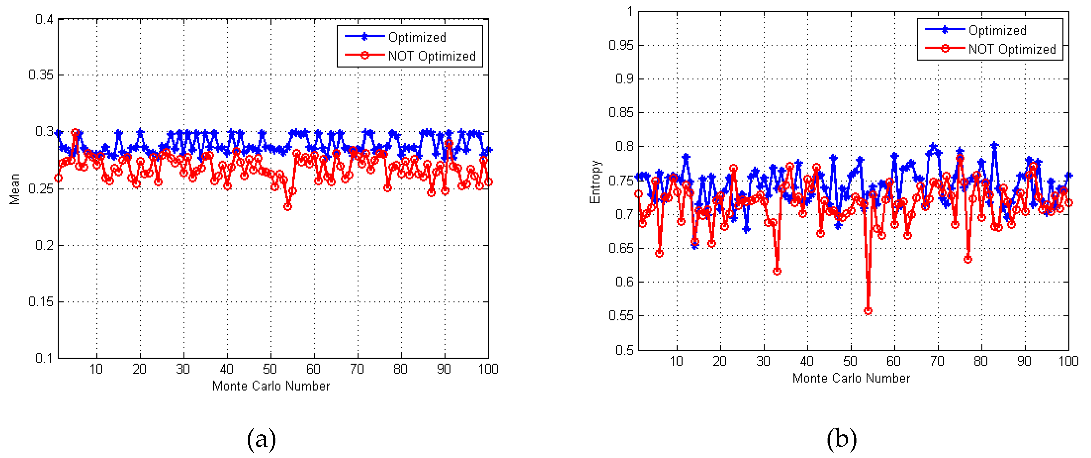
5.7. Statistical Results of Different Optimized MPSM Jamming

The purpose of the simulation in this section was to verify the stability and repeatability of the MPSM optimization algorithm jamming based on PSO, which contributes to the application of MPSM jamming. Taking four sections of MPSM jamming as an example, 100 Monte Carlo simulation experiments were completed for different optimized MPSM jamming.

5.7.1. Optimized Section Situation

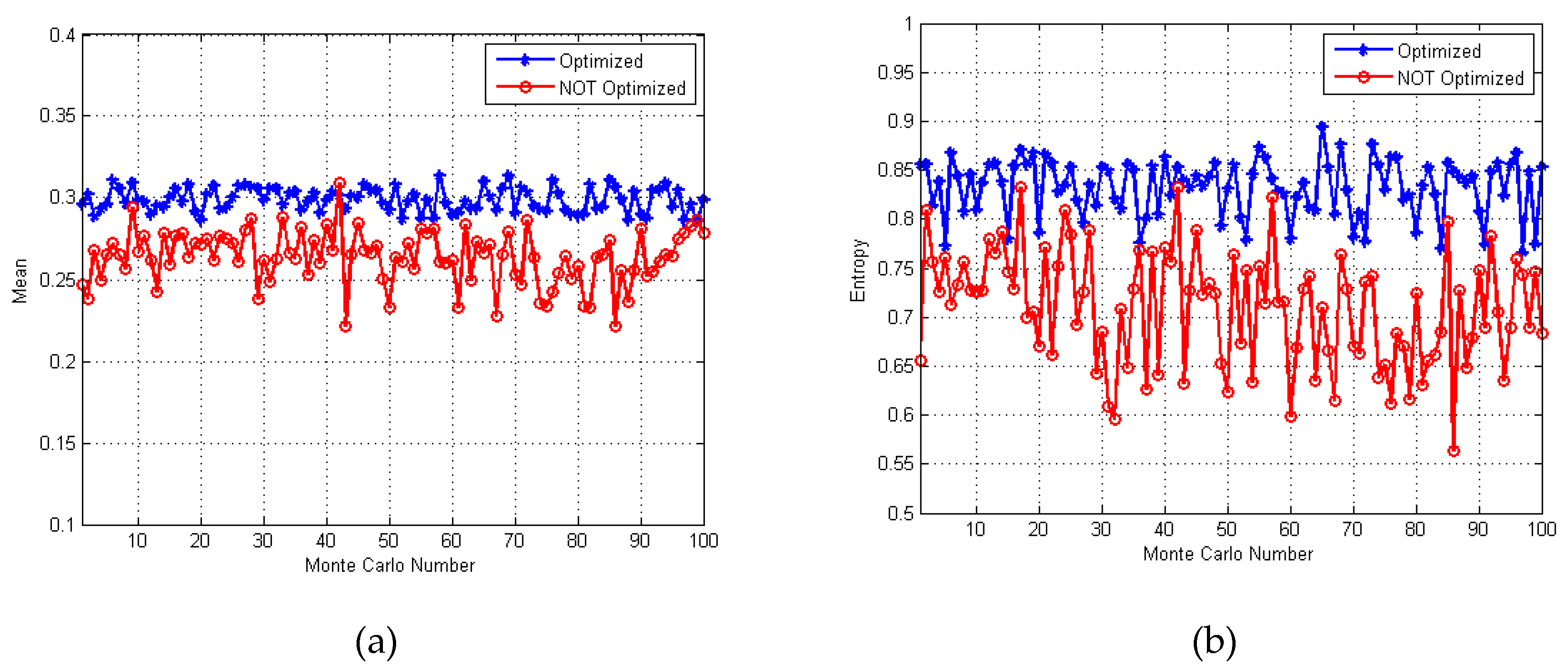
The simulation in this section was the result of MPSM jamming under the optimized section situation and MPSM jamming under the random section situation as the control group, where the phase situation was 0.095π, 0.685π, 1.472π, and 1.589π. Figure 19a provides the mean values of the simulation, and Figure 19b is the entropy values of the simulation. The blue curves are the results of MPSM jamming under optimized section situation, and the red curves are the results of MPSM jamming under the random section situation.

In Figure 19a, the mean values for the optimized section situation are almost higher than the mean values for the random section situation, and the curve for the optimized section situation is more stable than that for the random section situation. In Figure 19b, the entropy values of the optimized section situation are a little larger than the entropy values of the random section situation, and the curve for the optimized section situation is slightly more stable than the curve for the random section situation.

The mean and variance of the curves in Figure 19 were calculated and are shown in

Table 14. Mean and variance of curves in Figure 19.

Figure 19	Mean		Variance
	Random	Optimized	Random	Optimized
(a)	0.268	0.288	0.011	0.008
(b)	0.714	0.741	0.034	0.028

. In Table 14, the means of the blue curves are higher than the means of the red curves in Figure 19a,b, which means that the result of MPSM jamming for the optimized section situation performs better on average, and the variances of the blue curves are lower than the variances of the red curves in Figure 19a,b, which means that the result of MPSM jamming for the optimized section situation is also more stable.

According to the analysis, MPSM jamming for the optimized section situation based on PSO has stability and repeatability, which contribute to the application of MPSM jamming.

5.7.2. Optimized Phase Situation

The simulation in this section is the result of MPSM jamming for the optimized phase situation and MPSM jamming for the random phase situation as a control group, where the section situation is 0.250, 0.315, 0.410, and 0.025. Figure 20a depicts the mean values of the simulation, and Figure 20b depicts the entropy values of the simulation. The blue curves are the results of MPSM for the optimized phase situation, and the red curves are the results of MPSM jamming for the random phase situation.

In Figure 20a, most of the mean values for the optimized phase situation are higher than those for the random phase situation. The curve for the optimized phase situation is highly stable, but the curve for the random phase situation highly fluctuates. In Figure 20b, the entropy values for the optimized phase situation are almost higher than the entropy values for the random phase situation, and the curve for the optimized phase situation is relatively stable, but the curve for the random phase situation highly fluctuates.

The mean and variance of the curves in Figure 20 were calculated and are shown in

Table 15. Mean and variance of curves in Figure 20.

Figure 20	Mean		Variance
	Random	Optimized	Random	Optimized
(a)	0.262	0.273	0.016	0.001
(b)	0.708	0.786	0.050	0.022

. In Table 15, the means of the blue curves are higher than those of the red curves, for both Figure 20a,b, which means that the result of MPSM jamming under the optimized phase performs better on average. The variances of the blue curves are lower than the variances of the red curves in both Figure 20a,b, which means that the result of MPSM jamming with optimized phase situation is much more stable.

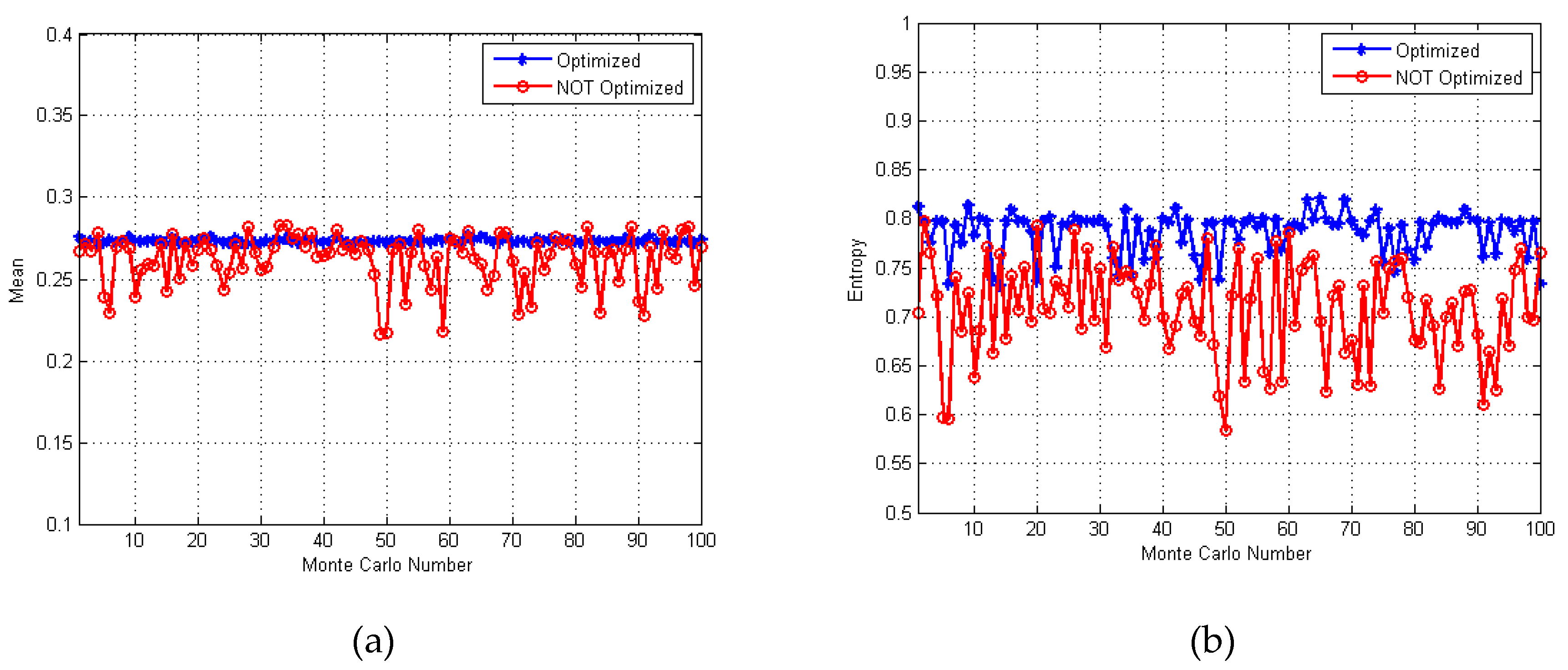
5.7.3. Optimized Section Situation and Phase Situation

The simulation in this section outlines the result of MPSM jamming for the optimized section situation and the phase situation, and MPSM jamming under the random section situation and the phase situation as control group. Figure 21a shows the mean values of the simulation, and Figure 21b provides the entropy values of the simulation. The blue curves are the results of MPSM jamming for the optimized section situation and the phase situation, and the red curves are the results of MPSM jamming for the random section situation and the phase situation.

In Figure 21a, all the mean values for the optimized section situation and the phase situation are higher than the mean values for the random section situation and phase situation, except for one point in Figure 21a. The curve for the optimized section situation and the phase situation is more stable than the curve for the random section situation and the phase situation. In Figure 21b, the entropy values for the optimized section situation and phase situation are all much higher than those for the random section situation and the phase situation. The curve for the optimized section situation and the phase situation is more stable than that for the random section situation and phase situation.

The mean and variance of the curves in Figure 21 were calculated and are shown in

Table 16. Mean and variance of curves in Figure 21.

Figure 21	Mean		Variance
	Random	Optimized	Random	Optimized
(a)	0.263	0.299	0.017	0.007
(b)	0.709	0.832	0.059	0.029

. In Table 16, the means of the blue curves are higher than those of the red curves in both Figure 21a,b, which means that the result of MPSM jamming under the optimized section situation and the phase situation performs better on average. The variances of the blue curves are lower than the variances of the red curves in both Figure 21a,b, which means that the result of MPSM jamming under the optimized section situation and the phase situation is more stable.

5.7.4. Summary

The means of the curves in Figure 19, Figure 20 and Figure 21 are shown in Table 16. In Table 16, the means of the mean value curve and entropy value curve of MPSM jamming for the optimized section and phase situation are the largest because MPSM jamming for the optimized section and phase situation had more variables than the others, which contributes more to higher degrees of freedom and mismatching with the original signal. This means that MPSM jamming for the optimized section and phase situation performs the best. MPSM jamming for the optimized section situation and MPSM jamming for the optimized phase situation produced better performance.

The variances of the curves in Figure 19, Figure 20 and Figure 21 are shown in

Table 17. Comparison of the means of curves.

Number in Figure 19, Figure 20 and Figure 21	Number of Sections	Section Situation	Phase Situation	Section Situation and Phase Situation
(a)	4	0.288	0.273	0.299
(b)	16	0.741	0.786	0.832

. In Table 17, the variances of the mean value curve and the entropy value curve of MPSM jamming for the phase situation are the smallest because MPSM jamming for the optimized phase situation has the fewest variables and the phase situation less influences the results compared to the section situation, which means MPSM jamming for the optimized phase situation is the most stable. MPSM jamming for the optimized section situation and MPSM jamming for the optimized section and phase situation are more stable.

In

Table 18. Comparison of the variances of the curves.

Number in Figure 19, Figure 20 and Figure 21	Number of Sections	Section Situation	Phase Situation	Section Situation and Phase Situation
(a)	4	0.008	0.001	0.007
(b)	16	0.028	0.022	0.029

, the variances of the curves in Figure 19, Figure 20 and Figure 21 show that the optimization algorithm for MPSM Jamming based on PSO has stability, which means that every result obtained from the optimization algorithm is in a small fixed range. The results in that small fixed range, to some extent, can be considered as the same value, which means that the optimization algorithm has repeatability.

6. Conclusions

First, we analyzed the principle of MPSM jamming, established mathematical modeling of MPSM jamming, deduced the equation for MPSM jamming after pulse compression, and reasonably simplified the equation. Then, we analyzed the influence of the section situation and the phase situation on MPSM jamming and concluded that the relationship between the results and parameter settings is difficult to determine. On this basis, an optimization algorithm for MPSM jamming based on PSO was proposed and studied. By setting an appropriate fitness function and a fitness value, as well as searching the section situation and phase situation that minimize the fitness function and fitness value, optimal local suppression MPSM jamming and its parameter settings were obtained. The optimization algorithm proposed in this paper can produce the optimal local suppression jamming result and its corresponding parameter settings with certain stability and repeatability, which further expands the practical application potential of MPSM jamming and provides some ideas for follow-up research.

References

- Spezio, A.E. Electronic warfare systems. IEEE Trans. Microw. Theory Tech. 2002, 50, 633–644. [Google Scholar] [CrossRef]
- Adamy, D. EW 101: A First Course in Electronic Warfare; Artech House: London, UK, 2001. [Google Scholar]
- Sun, Q.; Shu, T.; Yu, K.B. Efficient Deceptive Jamming Method of Static and Moving Targets against SAR. IEEE Sens. J. 2018, 18, 3610–3618. [Google Scholar] [CrossRef]
- Liu, Y.; Wang, W.; Pan, X. A frequency-domain three-stage algorithm for active deception jamming against synthetic aperture radar. IET Radar Sonar Navig. 2014, 8, 639–646. [Google Scholar] [CrossRef]
- Liu, Y.; Wang, W.; Pan, X. Influence of Estimate Error of Radar Kinematic Parameter on Deceptive Jamming Against SAR. IEEE Sens. J. 2016, 16, 5904–5911. [Google Scholar] [CrossRef]
- Wang, G.X.; Peng, S.R.; Sun, J.J. Effect evaluation for SAR suppression jamming based on edge strength image. In Proceedings of the IET International Radar Conference 2015, Hangzhou, China, 14–16 October 2015. [Google Scholar]
- Jiang, J.; Wu, Y.; Wang, H. Analysis of active noise jamming against synthetic aperture radar ground moving target indication. In Proceedings of the International Congress on Image & Signal Processing, Shenyang, China, 14–16 October 2015. [Google Scholar]
- He, J.; Peng, F.; Liu, Z. The Analysis of Noise Frequency Modulation Jamming Signal Based on Stochastic Differential. In Proceedings of the International Conference on Computer Application and System Modeling, Taiyuan, China, 7 July 2012. [Google Scholar]
- Guo, J.; Wang, X.; Xing, W. New smart noise jamming of radar signal frequency modulation. J. Xidian Univ. 2013, 40, 155–160. [Google Scholar] [CrossRef]
- Zhu, N.L.; Liu, H.L. Research into the Influence of Frequency Shift on Smart Noise Jamming with Convolution Modulation. Shipboard Electron. Countermeasure 2016, 39, 17–20. [Google Scholar] [CrossRef]
- Zhao, J.-y.; Liu, X.-w.; Yang, G. Research into Modeling and Jamming Methods of High Precision Phased Array Early Warning Radar Signal. Shipboard Electron. Countermeasure 2018, 37–41. [Google Scholar] [CrossRef]
- Shi, Z.Y.; Wang, M.; Zhang, L.; Ma, L.Z. A smart interference method based on trapezoidal wave convolution modulation. J. Airf. Early Warn. Acad. 2018, 48–54. [Google Scholar]
- Yuan, T.; Tao, J.F.; Li, X.C. Research on Convolution Jamming Technique Based on Triangle Wave Modulation. Meas. Control Technol. 2017, 36, 42–46. [Google Scholar] [CrossRef]
- Dong, H.L.; Xie, L.; Ren, G.H. Concluding and Analysis of Dense False Targets Producing Method by Using Convolution-Modulated Jamming. Fire Control Radar Technol. 2016, 45, 31–34. [Google Scholar] [CrossRef]
- Jiang, J.-w.; Wu, Y.-h.; Wang, H.-y.; Chen, J.-b. A Dense False Target Jamming Technique against SAR-GMTI. Shipboard Electron. Countermeasure 2016, 39, 9–14. [Google Scholar] [CrossRef]
- Hao, H.; Zeng, D.; Ge, P. Research on the Method of Smart Noise Jamming on Pulse Radar. In Proceedings of the Fifth International Conference on Instrumentation and Measurement, Computer, Communication and Control, Qinhuangdao, China, 18–20 September 2016. [Google Scholar]
- Tang, L.; Li, S. Application research on scatter-wave jamming for spaceborne SAR. Aerosp. Electron. Warfare 2016, 32, 34–36. [Google Scholar] [CrossRef]
- Hu, H.; Jia, X.; Wu, Y.; Wu, J. Research on the Theory of 2-D Interrupted Sampling Repeater Scatter-wave Jamming to SAR. J. Acad. Equip. Command Technol. 2012, 23, 94–97. [Google Scholar] [CrossRef]
- Wang, D.; Qu, F.; Jiao, J. Generation of scatter-wave jamming signal to SAR and jamming effects analysis. Aerosp. Electron. Warfare 2013, 29, 27–30. [Google Scholar] [CrossRef]
- Hu, D.; Wu, Y. The Scatter-Wave Jamming to SAR. Acta Electron. Sin. 2002, 30, 1882–1884. [Google Scholar] [CrossRef]
- Li, T.; Chen, W.; Lu, G.; Wang, D.J. A Study on Scatter-Wave Jamming for Countering SAR. In Proceedings of the International Conference on Microwave and Millimeter Wave Technology, Guilin, China, 18–21 April 2007. [Google Scholar]
- Wang, C.; Zhu, H.; Pan, Y.J.; Yuan, N.C. Novel noise jamming method against ISAR. In Proceedings of the IET International Radar Conference 2015, Hangzhou, China, 14–16 October 2015. [Google Scholar]
- Daobin, Y.; Yanhong, W.; Wang, H.; Xin, J. Research on Multiple Phase Sectionalized Modulation Jamming Method for Inverse Synthetic Aperture Radar. J. Electron. Inf. Technol. 2017, 39, 423–429. [Google Scholar] [CrossRef]
- Yu, D.B.; Wu, Y.H.; Jia, X.; Wang, H.Y. Research on Multiple Phase Sectionalized Modulation Jamming Method for Pulse Compression Radar. J. Signal Process. 2016, 32, 1178–1186. [Google Scholar] [CrossRef]
- Sun, Y.X.; Qi, G.Y.; Wang, Z.H.; Barend, J. Chaotic particle swarm optimization. In Proceedings of the Genetic and Evolutionary Computation Conference, Shanghai, China, 28–30 March 2010. [Google Scholar]
- Coello, C.A.C.; Pulido, G.T.; Lechuga, M.S. Handling multiple objectives with particle swarm optimization. IEEE Trans. Evol. Comput. 2004, 8, 256–279. [Google Scholar] [CrossRef]
- Lu, Z.Y.; Li, X.P.; Chen, Q.; Zou, X.H. Kalman filtering decoupling algorithm based on particle swarm optimization. Syst. Eng. Electron. 2018, 751–755. [Google Scholar] [CrossRef]
- Yang, Q.; Sun, S. Radar emitter recognition based on particle swarm optimization algorithm. Laser J. 2018, 118–121. [Google Scholar] [CrossRef]
- Buonamici, F.; Carfagni, M.; Furferi, R.; Governi, L.; Lapini, A.; Volpe, Y. Reverse Engineering of Mechanical Parts: A Template-Based Approach. J. Comput. Des. Eng. 2017, 5, 145–159. [Google Scholar] [CrossRef]
- Ines, A.V.M.; Honda, K.; Gupta, A.D.; Droogers, P.; Celemente, R.S. Combining remote sensing-simulation modeling and genetic algorithm optimization to explore water management options in irrigated agriculture. Agric. Water Manag. 2006, 83, 221–232. [Google Scholar] [CrossRef]
- Monteiro, R.P.; Lima, G.A.; Oliveira, J.P.G.; Cunha, D.S.C.; Bastos-Filho, C.J.A. Accelerating the convergence of adaptive filters for active noise control using particle swarm optimization. In Proceedings of the 2017 IEEE Latin American Conference on Computational Intelligence, Arequipa, Peru, 8–10 November 2017. [Google Scholar]
- Luo, H.; Jia, P.; Qiao, S.; Duan, S. Enhancing electronic nose performance based on a novel QPSO-RBM technique. Sens. Actuators, B 2018, 259, 241–249. [Google Scholar] [CrossRef]
- Bashir, Z.A.; El-Hawary, M.E. Applying Wavelets to Short-Term Load Forecasting Using PSO-Based Neural Networks. IEEE Trans. Power Syst. 2009, 24, 20–27. [Google Scholar] [CrossRef]
- Ishaque, K.; Salam, Z.; Amjad, M.; Mekhilef, S. An Improved Particle Swarm Optimization (PSO)–Based MPPT for PV With Reduced Steady-State Oscillation. IEEE Trans. Power Electron. 2012, 27, 3627–3638. [Google Scholar] [CrossRef]
- Shi, Y.; Eberhart, R.C. Parameter Selection in Particle Swarm Optimization. In Proceedings of the International Conference on Evolutionary Programming VII, San Diego, USA, 25–27 March 1998. [Google Scholar]
- Trelea, I.C. The particle swarm optimization algorithm: Convergence analysis and parameter selection. Inf. Process. Lett. 2003, 85, 317–325. [Google Scholar] [CrossRef]
Figure 1.
Received radar signal.
Figure 2.
Received radar signal after multiple phases sectionalized modulation (MPSM).
Figure 3.
Sketch map of envelope with equal section lengths. The rectangles with blue lines are sketch maps of the envelope of four sections after MPSM.
Figure 4.
Sketch map of envelope with random section lengths. The rectangles with blue lines are sketch maps of the envelope of four sections after MPSM.
Figure 5.
Sketch map of summation with equal section lengths and random phase situation. The black arrows represent the vectors of four sections after MPSM, and the red arrow represents the summation of black arrows.
Figure 6.
Sketch map of summation with random section length and random phase situation. The black arrows represent the vectors of four sections after MPSM, and the red arrow represents the summation of black arrows.
Figure 7.
Convergence domain of particle swarm optimization (PSO).
Figure 8.
Flowchart of optimization algorithm.
Figure 9.
Convergence with different inertia weights.
Figure 10.
Convergence with different acceleration coefficients.
Figure 11.
Convergence with different population sizes.
Figure 12.
Convergence of PSO and genetic algorithm (GA).