Multi-Sensor Optimization Scheduling for Target Tracking Based on PCRLB and a Novel Intercept Probability Factor

Abstract

In order to improve the survivability of active sensors, the problem of low probability of intercept (LPI) for a multi-sensor network system is studied in this paper. Two kinds of operational requirements are taken into account, the first of which is to ensure the survivability of sensors and the second is to improve the tracking accuracy of targets as much as possible. Firstly, the sensor tracking model and the posterior Carmér-Rao lower bound (PCRLB) of the target are presented to evaluate the sensor tracking benefits in next time. Then, a novel intercept probability factor (IPF) is proposed for multi-sensor multi-target tracking scenarios. At the basis of PCRLB and IPF, a myopic multi-sensor scheduling model for target tracking is set up to control the intercepted probability of sensors and improve the target tracking accuracy. At last, a fast solution algorithm based on an improved particle swarm optimization (PSO) algorithm is given to obtain the optimal scheduling actions. Simulation of experimental results show that the proposed model can effectively control the intercepted risk of every sensor, which can also obtain better target tracking performance than existing multi-sensor scheduling methods.

1. Introduction

In recent decades, multi-sensor networks have been widely used in many fields [1,2,3,4,5], such as battlefield surveillance, traffic control, healthcare, and environment monitoring. As a typical application in battlefield surveillance, target tracking by multi-sensor networks has been a research hotspot in recent years, especially in modern network warfare. Multi-sensor resource management has been proved to improve the performance of multi-sensor systems effectively. Multi-sensor resource management technology is able to make full use of sensor ability by scientific and reasonable scheduling of sensor resources [3]. By collaborative management of multi-sensor resources, the detection range and target tracking accuracy of the sensor network can be expanded.

However, when the active sensor detects a target, it will radiate the electromagnetic wave outward, which can expose itself [6]. At the same time, with the development of electronic technology, many anti-radiation weapons have been invented to attack active sensors, which poses a great challenge to the battlefield survivability of active sensors, especially radars. Therefore, the traditional sensor scheduling method, which only maximizes target tracking accuracy in most research, can no longer meet the operational requirements of the complex battlefield environment. When improving target tracking accuracy, the survivability of sensor network should also be considered. It requires us to study new sensor scheduling methods considering both target tracking accuracy and battlefield survivability.

Currently, there are four existing methods for active sensors to counter anti-radiation weapons: LPI waveform design technology [6,7,8], bistatic and distributed sensor technology [9,10], decoy and jamming technology [11], and sensor management technology [12,13,14]. Among them, the sensor management technology works through the cooperative work of multiple sensors. To realize the low intercepted probability of sensors, the key idea of sensor management technology is dynamically managing the existing sensor resources. It gives anti-radiation weapons difficulty in identifying the sensor or tracking the sensor for a long, continuous time. In this way, the anti-radiation weapon will not be able to position sensors or attack sensors further. This technology can reduce the intercepted probability of active sensors without increasing the hardware cost, which has become a research hotspot in this field. Reference [13] proposed a LPI controlling method based on Bhattacharyya distance and Jeffreys divergence, which can effectively control the intercepted risk of the whole radar network by reasonably allocating the radar working power. In [14], a low interception probability control method for multi-sensor networks based on mutual information entropy was presented. In [15,16], the radiation degree is used to quantify the intercepted risk of sensors. The radiation risk and the tracking accuracy are considered by information fusion method. However, combination of radiation risk and tracking precision is a single index. It is difficult to ensure that both of them can reach the ideal value. Secondly, the selection of the balance coefficient is very difficult without a priori knowledge.

However, previous work has focused only on controlling the intercepted risk of the whole sensor network without considering the survivability of single sensors. When the intercept probability of a multi-sensor network is small, the intercept probability of single sensor may already be very great, which is a potential security hazard. Besides, the target tracking accuracy is usually ignored in existing methods.

In view of the above problems, considering the survivability of every sensor, the problem of LPI controlling for multi-sensor multi-target tracking is addressed in this paper. This paper introduces a multi-sensor scheduling method based on posterior Carmér-Rao lower bound (PCRLB) and novel intercept probability factor (IPF). The method can ensure low intercept risk of every sensor while minimizing the target tracking accuracy as much as possible. Simulation results show that the proposed method can effectively control the intercepted probability of sensors within the security threshold, and can also maintain the target tracking accuracy at a higher level.

The rest of this paper is organized as follows. Firstly, the problem formulation is described in Section 2, and the target tracking model and PCRLB of the target state are given in Section 2.1 and Section 2.2, respectively. In Section 3, a novel intercept probability factor is proposed. Based on the analysis in Section 2 and Section 3, we present a multi-sensor scheduling model in Section 4. Then, a fast solution algorithm of sensor scheduling problems is put forward in Section 5. Section 6 presents some simulation results for different scenarios. Finally, conclusions and future works are discussed in Section 7.

2. Problem Formulation

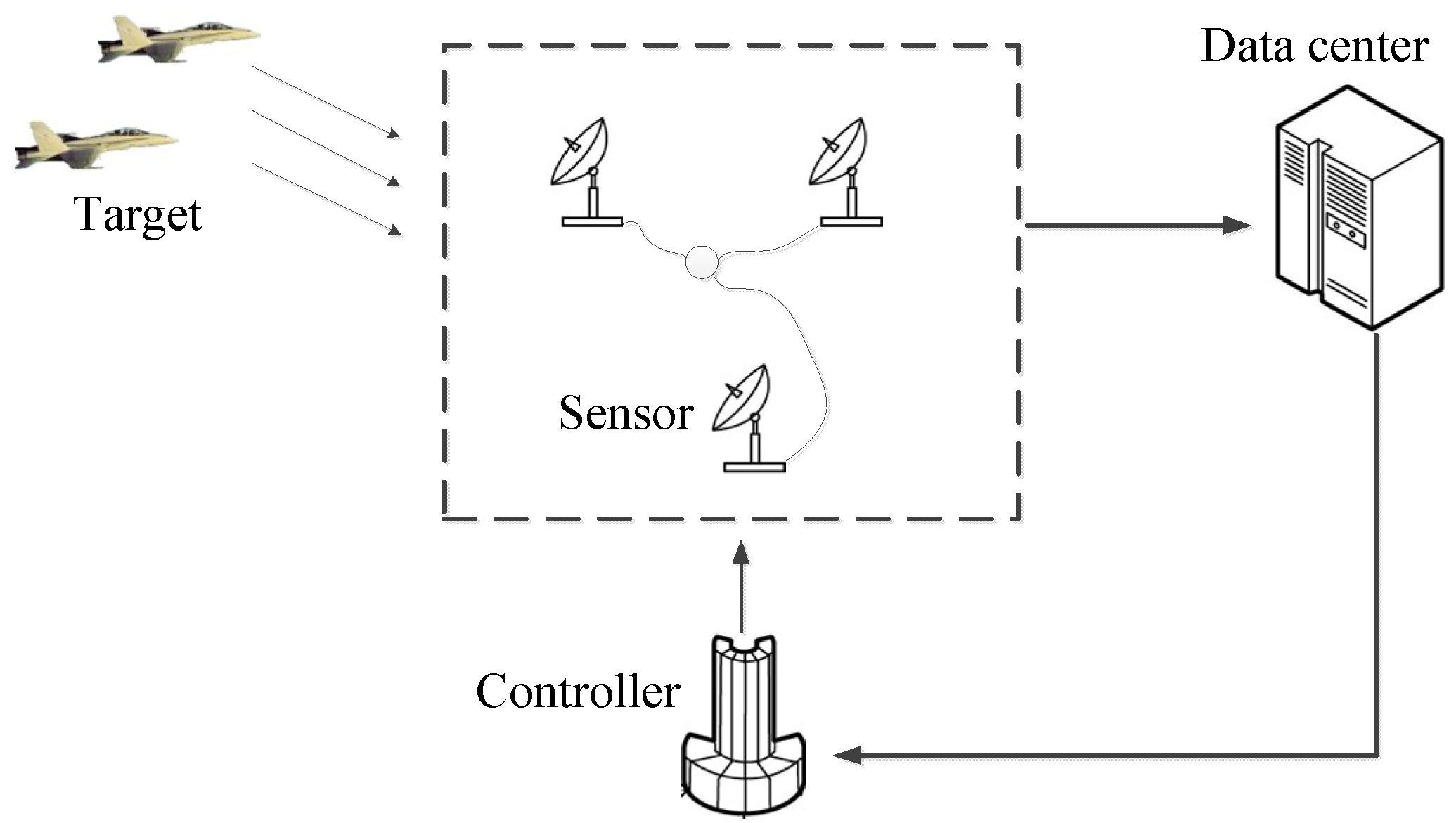
With the development of electronic technology, there are many sensors in air defense systems, such as radar, infrared detectors, and video trackers. As is shown in Figure 1, the main objective of this paper is to investigate the multi-sensor scheduling method for multi-target tracking. We assume that the centralized management method is utilized to manage multi-sensor resources, and the target information obtained by every sensor can be shared with the control center. The following parts in this section are the target tracking model and optimization objectives of multi-sensor scheduling.

2.1. Target Tracking Model

Supposing that there are $N$ active sensors distributed in a sensor field to track $M$ targets in two-dimensions space. Then, the target tracking mode in discrete time can be described as Equation (1).

$${\mathit{x}}_{}^m(k)={\mathit{F}}^m\cdot {\mathit{x}}_{}^m(k-1)+{\mathsf{\Gamma }}^m\cdot {\mathit{\nu }}_{}^m(k)$$

(1)

where the $\mathit{x}$ is target state, the state of target $m(m=1,2,\dots M)$ at time k is ${\mathit{x}}_{}^m(k)={[x_{}^m(k){\dot{x}}_{}^m(k)y_{}^m(k){\dot{y}}_{}^m(k)]}^{\mathrm{T}}$, and $x_{}^m(k)$, ${\dot{x}}_{}^m(k)$ denotes the position and speed at $x$ direction; $y_{}^m(k)$, ${\dot{y}}_{}^m(k)$ denote the position and speed at $y$ direction, respectively. ${\mathit{F}}^m$ is the state transition matrix, ${\mathsf{\Gamma }}^m$ and ${\mathit{\nu }}^m$ are the noise gain matrix and target state transition noise, which is Gauss white noise with zero mean and covariance $\mathit{Q}$. For a maneuvering target, the motion model of the target is unknown. Thus, the system state transition law is described by a mixed motion model set $\left\{{\mathit{F}}_{}^i\right\}$ $i=1,2,\dots ,\eta$, where $\eta$ is the number of motion models, and there is ${\mathit{F}}_{}^m\in \left\{{\mathit{F}}_{}^i\right\}$. There are three common motion models: the nearly constant velocity (NCV) model, nearly left constant turn (NLCT) model, and nearly right constant turn (NRCT) model. The state transition matrices of NCV model and NCT model can be described as

$${\mathit{F}}_{\mathrm{cv}}^{}=\left[\begin{array}{cccc}1& T_s& 0& 0\\ 0& 1& 0& 0\\ 0& 0& 1& T_s\\ 0& 0& 0& 1\end{array}\right],{\mathit{F}}_{\mathrm{CT}}^{}=\left[\begin{array}{cccc}1& \sin \omega T_s/\omega & 0& -\left(1-\cos \omega T_s\right)/\omega \\ 0& \cos \omega T_s& 0& \sin \omega T_s\\ 0& \left(1-\cos \omega T_s\right)/\omega & 1& \sin \omega T_s/\omega \\ 0& -\sin \omega T_s& 0& \cos \omega T_s\end{array}\right]$$

(2)

where $T_s$ is the sampling interval, $\omega$ denotes the turn rate of the target.

In general, the slope distance and azimuth angles are usually chosen as the measurement values of active sensors, and the measurement equation is as follows:

$${\mathit{z}}_{}^{m,n}(k)=h_{}^n\left({\mathit{x}}_{}^m(k)\right)+{\mathit{w}}_{}^n(k)=\left[\begin{array}{l}{r}_{}^{m,n}(k)\\ {\theta }_{}^{m,n}(k)\end{array}\right]+\left[\begin{array}{l}{w}_{}^{n,r}(k)\\ w_{}^{n,\theta }(k)\end{array}\right]$$

(3)

where $\mathit{z}$ represents the target measurement, $h_{}^n$ is a nonlinear measurement equation sensor $n(n=1,2,\dots N)$, $\mathit{w}$ is measurement noise which is also Gauss white noise with zero mean and covariance $\mathit{R}$; $w_k^{n,r}$, $w_k^{n,\theta }$ denote the measurement noise of slope distance $r_{}^{m,n}(k)$ and azimuth angle ${\theta }_{}^{m,n}(k)$, respectively. In particular, the calculation methods of $r_{}^{m,n}(k)$, ${\theta }_{}^{m,n}(k)$ are as shown in Equations (4) and (5), respectively.

$$r_{}^{m,n}(k)=\sqrt{{\left(x_{}^m(k)-x_s^n\right)}^2+{\left(y_{}^m(k)-y_s^n\right)}^2}$$

(4)

$${\theta }_{}^{m,n}(k)={\tan }^{-1}\frac{y_{}^m(k)-y_s^n}{x_{}^m(k)-x_s^n}$$

(5)

where $x_s^n$ and $y_s^n$ are position coordinates of sensor n.

2.2. PCRLB of Target State

The purpose of the sensor optimization scheduling in this paper is to reduce the risk of interception and achieve higher target tracking accuracy during the sensor scheduling process. Therefore, in order to select appropriate sensors to track targets in advance, it is necessary to predict and analyze the future tracking performance of sensors. By this approach, the control center can make a decision ahead of time. According to Equation (6), PCRLB can provide a lower bound of the estimation error of the target state without knowing the sensors real measurements in the future, which is suitable for the problem of sensor scheduling. Compared with Carmér-Rao lower bound (CRLB), PCRLB is more precise. That is because the measurement value can provide more target information. Therefore, PCRLB is used to evaluate the sensor tracking benefits in our study. In [17], PCRLB is defined to be the inverse of the posterior Fisher information matrix (FIM). Let ${\widehat{\mathit{x}}}_{k+1}^m$ be an unbiased estimator of ${\mathit{x}}_{k+1}^m$, and the PCRLB for the estimator ${\mathit{x}}_{k+1}^m$ satisfies the following inequality.

$$\mathsf{{\rm E}}\left\{\left[{\widehat{\mathit{x}}}_{k+1}^m-{\mathit{x}}_{k+1}^m\right]{\left[{\widehat{\mathit{x}}}_{k+1}^m-{\mathit{x}}_{k+1}^m\right]}^{\mathsf{{\rm T}}}\right\}\ge {\left({\mathit{J}}_{k+1}^m\right)}^{-1}$$

(6)

where ${\mathit{J}}_{k+1}^m$ is the posterior FIM, which meets the following recursive Equation (7).

$${\mathit{J}}_{k+1}^m={\mathit{D}}_k^{m,22}-{\mathit{D}}_k^{m,21}{\left({\mathit{J}}_k^m+{\mathit{D}}_k^{m,11}\right)}^{-1}{\mathit{D}}_k^{m,12}$$

(7)

and

$$\{\begin{array}{l}{\mathit{D}}_k^{m,11}=\mathsf{{\rm E}}[-{\nabla }_{{\mathit{x}}_k^m}^{{\mathit{x}}_k^m}\log p\left({\mathit{x}}_{k+1}^m|{\mathit{x}}_k^m\right)]\\ {\mathit{D}}_k^{m,12}={[{\mathit{D}}_k^{m,21}]}^{\mathsf{{\rm T}}}\\ =\mathsf{{\rm E}}[-{\nabla }_{{\mathit{x}}_k^m}^{{\mathit{x}}_{k+1}^m}\log p\left({\mathit{x}}_{k+1}^m|{\mathit{x}}_k^m\right)]\\ {\mathit{D}}_k^{m,22}=\mathsf{{\rm E}}[-{\nabla }_{{\mathit{x}}_{k+1}^m}^{{\mathit{x}}_{k+1}^m}\log p\left({\mathit{x}}_{k+1}^m|{\mathit{x}}_k^m\right)]+\\ \mathsf{{\rm E}}[-{\nabla }_{{\mathit{x}}_{k+1}^m}^{{\mathit{x}}_{k+1}^m}\log p\left({\mathit{z}}_{k+1}^{m,n}|{\mathit{x}}_{k+1}^m\right)]\end{array}$$

(8)

where ${\nabla }_{{\mathit{x}}_k^m}^{{\mathit{x}}_k^m}$ denotes the second-order partial derivatives, $\mathsf{{\rm E}}[-{\nabla }_{{\mathit{x}}_{k+1}^m}^{{\mathit{x}}_{k+1}^m}\log p\left({\mathit{z}}_{k+1}^{m,n}|{\mathit{x}}_{k+1}^m\right)]$ is the future information gain by the sensor measurements. For the model in Section 2.1, ${\mathit{D}}_k^{m,11}$, ${\mathit{D}}_k^{m,12}$, ${\mathit{D}}_k^{m,22}$ can be calculated by the following equations.

$$\{\begin{array}{l}{\mathit{D}}_k^{m,11}={\left({\mathit{F}}^m\right)}^{\mathsf{{\rm T}}}{\left({\mathit{Q}}^m\right)}^{-1}{\mathit{F}}^m\\ {\mathit{D}}_k^{m,12}=-{\left({\mathit{F}}^m\right)}^{\mathsf{{\rm T}}}{\left({\mathit{Q}}^m\right)}^{-1}\\ {\mathit{D}}_k^{m,22}={\left({\mathit{Q}}^m\right)}^{-1}+{\left({\mathit{H}}_{k+1}^n\right)}^{\mathsf{{\rm T}}}{\left({\mathit{R}}^n\right)}^{-1}{\mathit{H}}_{k+1}^n\end{array}$$

(9)

where ${\mathit{H}}_{k+1}^n$ is the Jacobi matrix of nonlinear measurement equation $h_{}^n$. Assuming that sensor n is used to track target m, the nonlinear measurement function is $h_{}^n\left({\mathit{x}}_{}^m(k+1)\right)$. It is known from Equations (2)–(4) that $h_{}^n\left({\mathit{x}}_{}^m(k+1)\right)$ can be rewritten as

$$h_{}^n\left({\mathit{x}}_{}^m(k+1)\right)=\left[\begin{array}{c}{r}_{}^{m,n}(k+1)\\ {\theta }_{}^{m,n}(k+1)\end{array}\right]=\left[\begin{array}{c}\sqrt{{\left(x_{}^m(k+1)-x_s^n\right)}^2+{\left(y_{}^m(k+1)-y_s^n\right)}^2}\\ {\tan }^{-1}\frac{y_{}^m(k+1)-y_s^n}{x_{}^m(k+1)-x_s^n}\end{array}\right]$$

(10)

and then the ${\mathit{H}}_{k+1}^{m,n}$ can be given by

$${\mathit{H}}_{k+1}^{m,n}=\left[\begin{array}{cc}\frac{\partial r_{}^{m,n}(k+1)}{\partial x}& \frac{\partial r_{}^{m,n}(k+1)}{\partial y}\\ \frac{\partial {\theta }_{}^{m,n}(k+1)}{\partial x}& \frac{\partial {\theta }_{}^{m,n}(k+1)}{\partial y}\end{array}\right]=\left[\begin{array}{c}\begin{array}{cc}\frac{x_{}^m(k+1)-x_s^n}{d_{mn}}& \frac{y_{}^m(k+1)-y_s^n}{d_{mn}}\end{array}\\ \begin{array}{cc}\frac{y_{}^m(k+1)-y_s^n}{{\left(d_{mn}\right)}^2}& \frac{x_{}^m(k+1)-x_s^n}{{\left(d_{mn}\right)}^2}\end{array}\end{array}\right]$$

(11)

where $d_{mn}$ is the Euclidean distance between sensor n and target m, and calculated method is given by

$$d_{mn}=\sqrt{{\left(x_{}^m(k+1)-x_s^n\right)}^2+{\left(y_{}^m(k+1)-y_s^n\right)}^2}$$

(12)

However, ${\mathit{x}}_{}^m(k+1)$ and $y_{}^m(k+1)$ are not known at time k. We can use ${\widehat{x}}_{}^m(k+1)$ and ${\widehat{y}}_{}^m(k+1)$ instead of ${\mathit{x}}_{}^m(k+1)$ and $y_{}^m(k+1)$. In this paper, according to the Equation (1), we use the one-step prediction value to approximate $x_{}^m(k+1)$ and $y_{}^m(k+1)$, and

$${\widehat{\mathit{x}}}_{}^m(k+1)={\mathit{F}}^m{\mathit{x}}_{}^m(k)$$

(13)

For maneuvering target, target motion model is unknown. Considering the continuity of target motion, the motion model corresponding to the maximum distribution probability at the current time is used as the target motion model, that is

$${\mathit{F}}_{}^m={\mathit{F}}_{}^i=\arg \underset{i=1,\dots ,\eta }{\max }{\mathit{\mu }}_k^i$$

(14)

where ${\mathit{\mu }}_k^i$ represents distribution probability of target motion model i at time k.

Here, the posterior FIM ${\mathit{J}}_{k+1}^{m,n}$ of target m from sensor n can be obtained by Equation (7). Furthermore, when N sensors are used to track the target m at the same time, assuming that the processes of sensor measurement are independent to each other, the measurement results will not interfere with each other. Then, the total posterior FIM ${\mathit{J}}_{k+1}^m$ can be expressed as

$${\mathit{J}}_{k+1}^m={\displaystyle \sum _{n=1}^N{\mathit{J}}_{k+1}^{m,n}}$$

(15)

In the process of target tracking, we pay more attention to the position of targets. Hence, the error boundary component of target position in ${\mathit{J}}_{k+1}^m$ is selected as the tracking benefits. Let ${\mathsf{\Upsilon }}_k\left({\mathit{X}}_k^{},{\mathit{A}}_{k+1}^{}\right)$ be the predicted tracking benefit function, which is given by

$$\begin{array}{l}{\mathsf{\Upsilon }}_k\left({\mathit{X}}_k^{},{\mathit{A}}_{k+1}^{}\right)\\ ={\displaystyle \sum _{m=1}^M\left\{{\left({\mathit{J}}_{k+1}^m\right)}^{-1}[1,1]+{\left({\mathit{J}}_{k+1}^m\right)}^{-1}[3,3]\right\}}\\ ={\displaystyle \sum _{m=1}^M\left\{{\left({\displaystyle \sum _{n=1}^N{a}_{mn}{\mathit{J}}_{k+1}^{m,n}}\right)}^{-1}[1,1]+{\left({\displaystyle \sum _{n=1}^N{a}_{mn}{\mathit{J}}_{k+1}^{m,n}}\right)}^{-1}[3,3]\right\}}\end{array}$$

(16)

where ${\mathit{X}}_k^{}=\left\{{\mathit{X}}_k^1,{\mathit{X}}_k^2,\dots ,{\mathit{X}}_k^M\right\}$, and $A_{k+1}$ represent the scheduling actions of sensors at time k+1, $A_{k+1}={[a_{mn}^{}]}_{MN}$, $a_{mn}^{}\in \{0,1\}$, which denotes that the sensor n is used to track target m when $a_{mn}=1$; the sensor n is not used to track target m when $a_{mn}=0$.

3. Novel Intercept Probability Factor

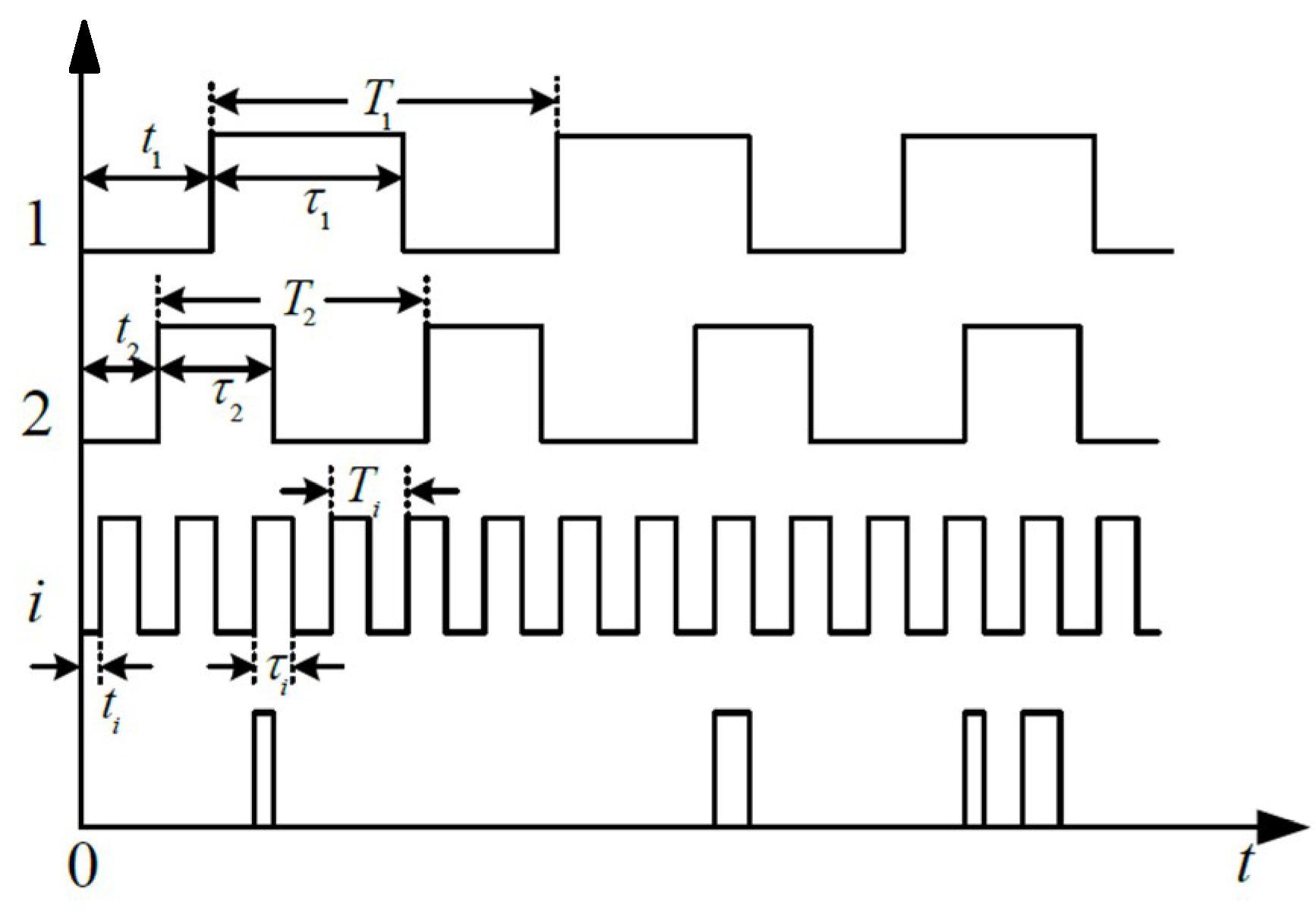
In an actual battlefield environment, even the signal power of a sensor is very high, and an anti-radiation weapon may not be able to intercept the sensor signal. As is shown in Figure 2, an interception event will occur only when overlaps happen to multiple window functions [18,19]. Here, in the process of intercepting, four window functions are considered for experimentation, which include the window functions of search direction and pulse signal for a sensor, and the window functions of search direction and search frequency for an anti-radiation weapon.

It is assumed that the width of each window is ${\tau }_i$ and the repetition interval of each window is $T_i$. Then, the coincident width of L windows at the same time is $\frac{1}{{\overline{\tau }}_0}={\displaystyle \sum _{i=1}^L\frac{1}{{\tau }_i}}$, and the coincident repetition interval is given by

$${\overline{T}}_0={\displaystyle \prod _{i=1}^L\left(T_i/{\tau }_i\right)}/{\displaystyle \sum _{i=1}^L\left(1/{\tau }_i\right)}$$

(17)

We now analyze the probability of an interception event for a sensor. Because the interception event has independence and is without after-effect, Poisson distribution can effectively describe the process of an interception event. Assuming that k coincidental events of L windows happened in t time, the probability of an interception event is obtained by

$$\{\begin{array}{c}P(T_0,k)=P_0\frac{{(P_0/{\overline{T}}_0)}^{k-1}}{(k-1)!}{\mathrm{e}}^{-t/{\overline{T}}_0}s+(1-P_0)\frac{{(t/{\overline{T}}_0)}^k}{k!}{\mathrm{e}}^{-t/{\overline{T}}_0}\\ P(t,0)=(1-P_0){\mathrm{e}}^{-t/{\overline{T}}_0},t\ge 0,k=1,2,3\dots \end{array}$$

(18)

where $P_0$ is the probability of an interception event in the initial time. When the number of coincidental events is k or more than k, the interception event will happen, then the probability $P_k(t)$ of k interception events can be calculated as

$$P_k(t)={\displaystyle \sum _{i=k}^{\infty }P(t,i)}=1-{\displaystyle \sum _{i=0}^{k-1}P(t,i)}$$

(19)

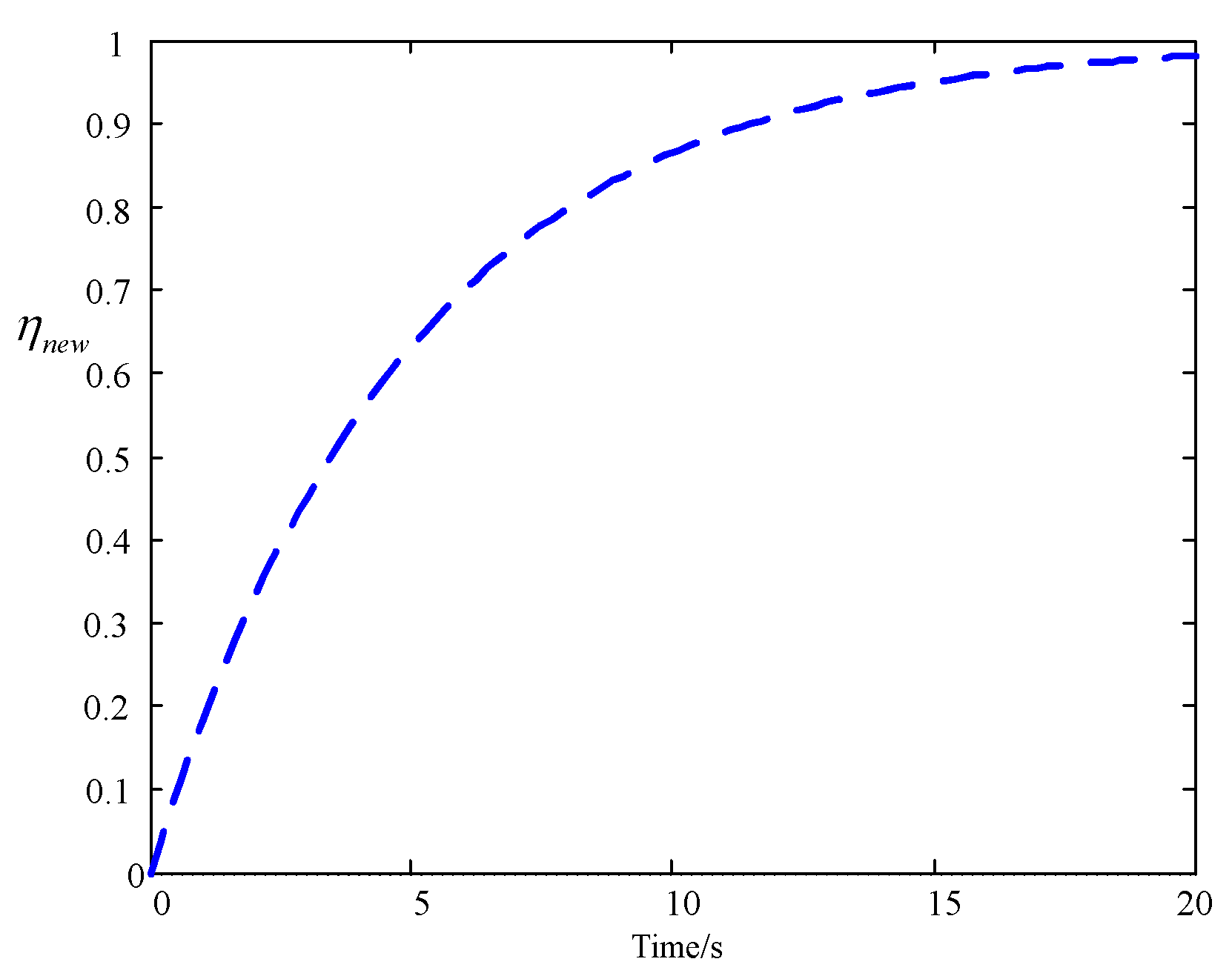
On further simplification in actual cases, when k = 1, the interception event will happen. Let the novel interception probability factor (IPF) ${\eta }_{new}$ be equal to $P_k(t)$ when k = 1, the ${\eta }_{new}$ is given by

$${\eta }_{new}=P_1(t)={\displaystyle \sum _{i=1}^{\infty }P(t,i)}=1-P(t,0)=1-(1-P_0){\mathrm{e}}^{-t/{\overline{T}}_0}$$

(20)

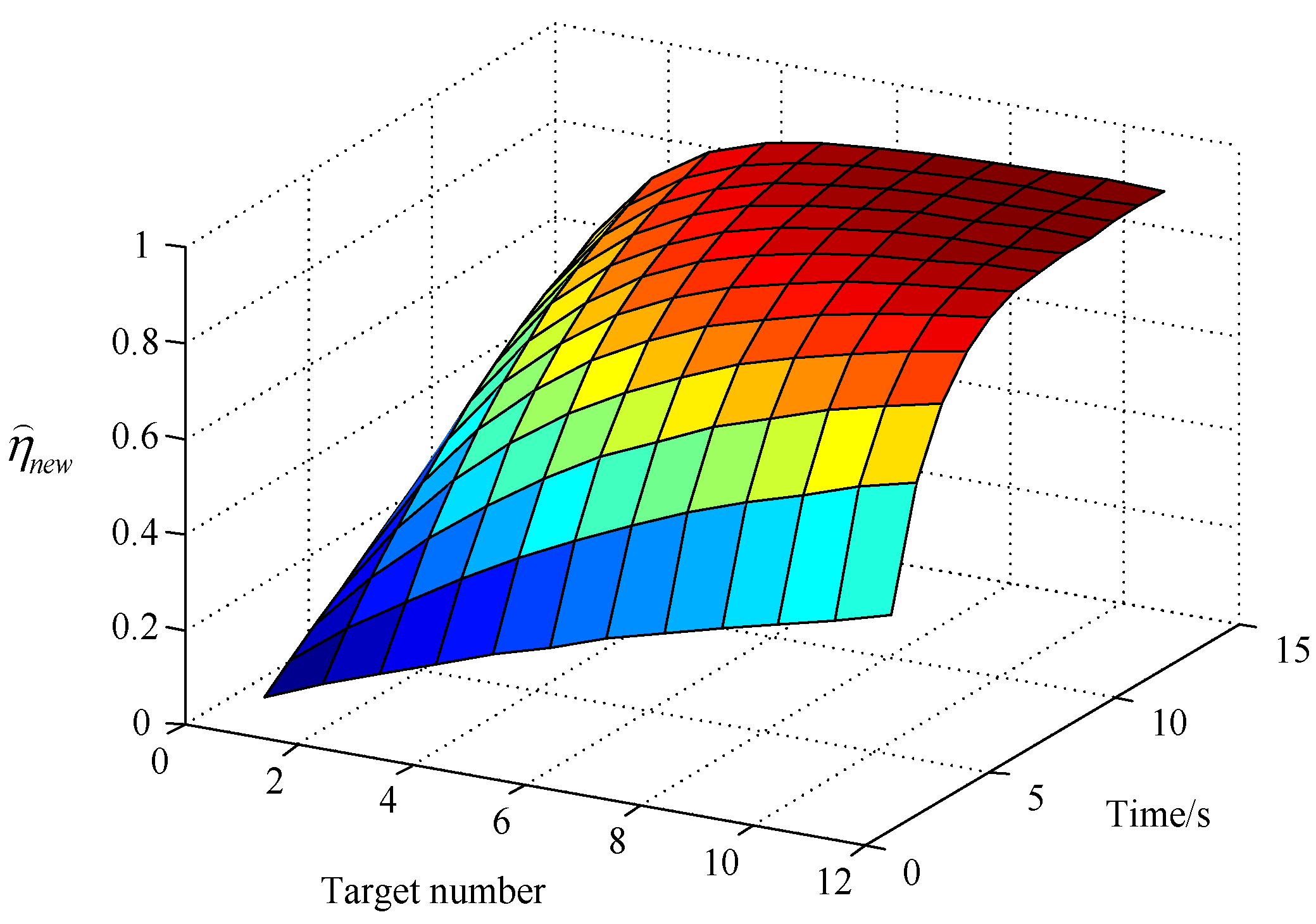
In general, $P_0\approx 0$, then ${\eta }_{new}$ can be simplified as ${\eta }_{new}\approx 1-{\mathrm{e}}^{-t/{\overline{T}}_0}$. When $T_0=5$, the change curve of ${\eta }_{new}$ is shown in Figure 3. It can be seen that the new IPF ${\eta }_{new}$ is a time-dependent function. The longer the tracking time is, the greater the ${\eta }_{new}$ is. Moreover, if the target number is M, the joint IPF ${\stackrel{⌢}{\eta }}_{new}$ is given by

$${\stackrel{⌢}{\eta }}_{new}=1-{\displaystyle \prod _{i=1}^M(1-{\eta }_{new}^i)}\approx 1-{\displaystyle \prod _{i=1}^M[1-(1-{\mathrm{e}}^{-t/{\overline{T}}_0})]}=1-{\mathrm{e}}^{-Mt/{\overline{T}}_0}$$

(21)

Figure 4 shows change curves of joint IPF ${\stackrel{⌢}{\eta }}_{new}$ when a sensor is used to track more than one target at the same time. It can be seen that the intercepted probability by anti-radiation weapon will further increase when the targets number increases. Therefore, in the process of target tracking, we should not only control the tracking time of the same sensor, but also try to avoid tracking multiple targets with the same sensor.

4. Multi-Sensor Scheduling Model

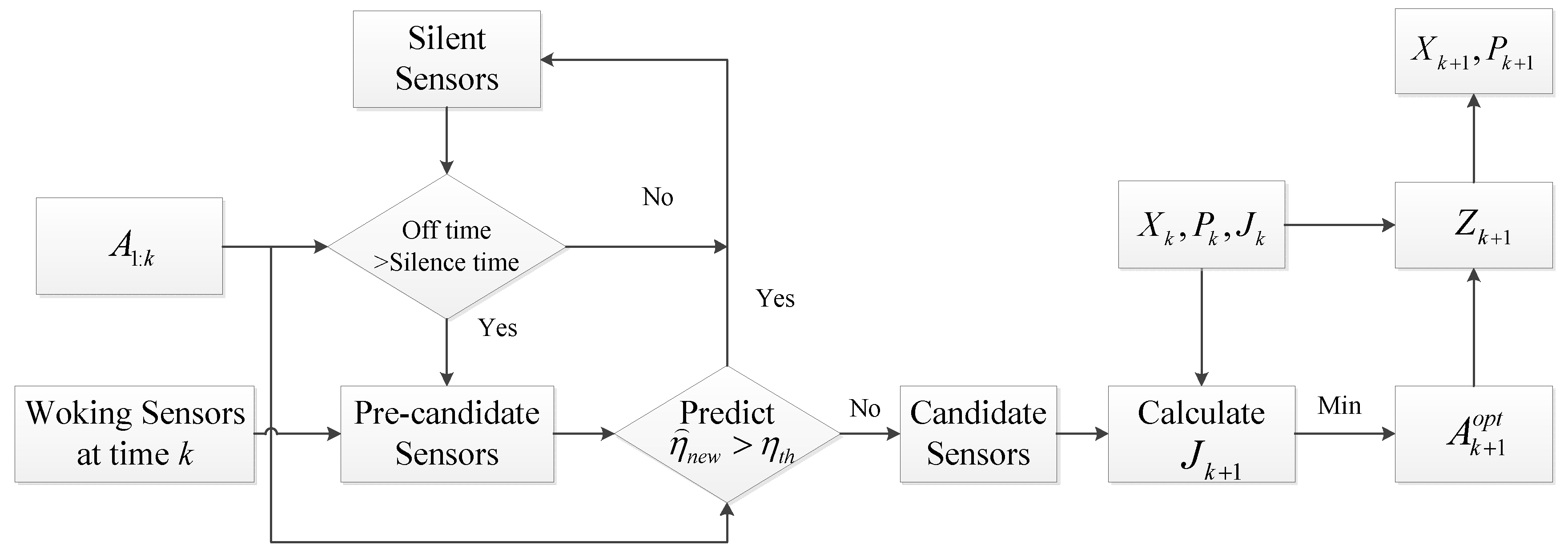
Based on the research in the above sections, considering PCRLB and the novel IPF, a multi-sensor scheduling model is set up. The basis of the proposed model is evaluating the joint IPF ${\stackrel{⌢}{\eta }}_{new}$ of sensors at each time. If the ${\stackrel{⌢}{\eta }}_{new}$ is greater than the intercepted probability threshold ${\eta }_{th}$, this sensor will quit tracking targets and maintain silence for a period of time. After the silence, this sensor will return to tracking targets. It is noted that the silence time is set up according to the actual battlefield requirement. Then, in the rest sensor group, the sensor scheduling scheme which has the smallest PCRLB will be selected in next time. At this point, the multi-sensor scheduling problem has been converted into the following optimization mathematical problem.

$$\{\begin{array}{c}{A}_{k+1}^{opt}=\arg \underset{A_{k+1}}{\min }{\mathsf{\Upsilon }}_k\left({\mathit{X}}_k^{},{\mathit{A}}_{k+1}^{}\right)={\displaystyle \sum _{m=1}^M\left\{{\left({\displaystyle \sum _{n=1}^N{a}_{mn}{\mathit{J}}_{k+1}^{m,n}}\right)}^{-1}[1,1]+{\left({\displaystyle \sum _{n=1}^N{a}_{mn}{\mathit{J}}_{k+1}^{m,n}}\right)}^{-1}[3,3]\right\}}\\ s.t.\{\begin{array}{l}{\displaystyle \sum _{n=1}^N{a}_{mn}^k\le }{C}_n,{\displaystyle \sum _{m=1}^M{a}_{mn}^k\le }{C}_m,{\stackrel{⌢}{\eta }}_{new}^n\le {\eta }_{th}\\ m=1,2,\dots ,M,n=1,2,\dots ,N\end{array}\end{array}$$

(22)

where $\mathsf{\Upsilon }\left({\mathit{X}}_k^{},{\mathit{A}}_{k+1}^{}\right)$ is the comprehensive tracking benefit, ${\eta }_{th}$ is the intercepted probability threshold, ${\stackrel{⌢}{\eta }}_{new}^n$ is the intercepted probability of sensor n, and $C_m$ is the maximum number of sensors allowed to track the same target m, $C_n$ is the tracking ability of sensor n. The specific steps of the multi-sensor with IPF scheduling model is shown in Algorithm 1, and the diagram of the multi-sensor scheduling process at time k is shown in Figure 5. To remind the reader, the sensor scheduling model proposed in this section is a myopic scheduling method, which only judges the tracking cost in next time. Compared with the non-myopic scheduling method, this method has less computation complexity and shorter optimization time, which can effectively meet the real-time requirement.

In order to quickly get the optimal scheduling actions ${\mathit{A}}_{k+1}^{opt}$, we will use a heuristic search algorithm [20] to deal with it in next section.

Algorithm 1 Multi-sensor scheduling algorithm

Input: target state ${\mathit{X}}_k^{}$, sensor scheduling actions ${\mathit{A}}_k^{}$ Output: sensor scheduling actions ${\mathit{A}}_{k+1}^{}$

Determine whether the silent sensors have reached the silence time For (sensor in silent group) If (off-time> silence time) silent sensors start work else silent sensors keep silence End End Predict the IPF of sensors which do not keep silence For (sensor which don’t keep silence) IF (Predictive IPF ${\stackrel{⌢}{\eta }}_{new}^n$ > ${\eta }_{th}$) Sensor will be not selected and turn to silence End End Select the sensor-target combination which has the smallest PCRLB Use particle swarm optimization (PSO) algorithm to search the optimal scheduling actions ${\mathit{A}}_{k+1}^{opt}$ Output sensor scheduling actions ${\mathit{A}}_{k+1}^{}$

5. Solution Algorithm of Multi-Sensor Scheduling Problem

According to Equation (22), by modeling, the sensor scheduling problem has been transformed into a nonlinear, multi-constrained NP-hard problem. In particular, when the numbers of sensors and targets are great, the computation complexity will increase greatly. It is very hard for traditional programming and analytic methods to solve this problem. Besides, the on-line planning must meet the real-time requirements. Therefore, a fast solution algorithm is needed. In response to the above problems, a fast solution algorithm based on the improved particle swarm optimization (PSO) algorithm is proposed. The PSO algorithm [21] is a kind of intelligent searching algorithm, which can obtain the optimal or suboptimal solution in a short time.

5.1. Solution Algorithm Based on Improved PSO Algorithm

The PSO algorithm [22] approximates the optimal solution by iterating a large number of particles. The renewal equation of particles is shown as

$$V^i(k+1)=w{V}^i(k)+c_1{r}_1[P_b^i(k)-P^i(k)]+c_2{r}_2[P_{gb}^i(k)-P^i(k)]$$

(23)

$$P^i(k+1)=P^i(k)+V^i(k+1)$$

(24)

where $P^i(k)$ is the position (hence the solution) of the ith particle at k time. It is a formal representation of the problem solution, which can be a vector or matrix. $V^i(k+1)$ is the movement speed of the ith particle, $P_b^i(k)$ is the best of ith particle in the iterative history, $P_{gb}^i(k)$ is the global best of all particles in the iterative history. $w,c_1,c_2$ are weight coefficients, and $w+c_1+c_2=1$, where $c_1$ represents the important degree of the individual experience during the iterative process, and $c_2$ represents the important degree of the group experience.

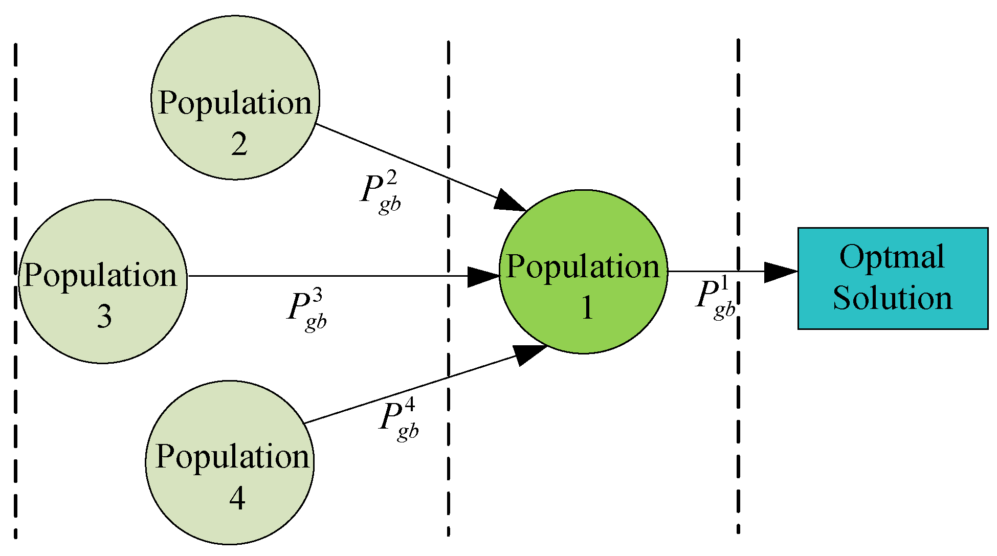
In PSO, the convergence of particles is so strong that particles are easy to fall into the local optimal trap. In response to the problem, a multi-population cooperative search strategy [23] is introduced to improve the optimization performance of the PSO algorithm. This strategy improves the PSO algorithm from a new perspective, whose key idea is using $L(L\ge 2)$ particle populations to search cooperatively. The L particle swarm is divided into two parts. The former $L-1$ particle populations search independently to expand the searching range, and the last particle population chases the global best solution of all particle populations to accelerate the convergence speed. Through cooperative searching by different populations, the global optimization ability of PSO will be improved significantly.

Here, we divide the particle swarm into four particle populations, as shown in Figure 6. Weight coefficients $w,c_1,c_2$ in particle populations 2, 3, and 4 are set up differently. Under the circumstances, different particle populations will have different searching ability. In particle population 2, the $w$ is greater than $c_1,c_2$, which means paying more attention to the value of the current particle itself. In particle population 3, the $c_1$ is greater than $w,c_2$, which means that the individual experience of the particle is considered greater. In particle population 4, the $c_2$ is greater than $w,c_1$, which means that the population experience is considered greater. Additionally, different particle populations can be computed in the parallel computing mode. In this way, a lot of computing time will be saved.

5.2. Particle Encoding in Improved PSO Algorithm

Particle encoding is the key technology in the improved PSO algorithm. A good encoding technique is helpful to improve the solving speed of the algorithm. Here, $P^i(k)$ is the exact sensor scheduling actions ${\mathit{A}}_k={[a_{mn}]}_{MN}$. Therefore, we can get ${\mathit{A}}_{k+1}^{opt}$ through iterative searching. It is important to note that the sensor scheduling actions are a binary discrete matrix. When the numbers of sensors and targets are both 3, the tracking capability $C_n$ of each sensor is 2, and the maximum number $C_m$ of sensors allowed to track the same target is 1; a legal example of ${\mathit{A}}_k^{}$ is shown in Equation (24).

$${\mathit{A}}_k^{}={\left[\begin{array}{ccc}0& 0& 1\\ 0& 0& 1\\ 1& 0& 0\end{array}\right]}_{3\times 3}$$

(25)

The sensor scheduling actions in Equation (25) denote that sensor 1 is used to track target 3, sensor 3 is used to track target 1 and target 2, and sensor 2 is not used. However, because Equations (23) and (24) are calculated in the real number space, the elements of ${\mathit{A}}_k^{}$ may become a real number out of {0, 1} during the iteration process. Therefore, the elements should be discretization and legalization during the iteration process. To solve the above problem, as is shown in Figure 7, a method of discretization and legalization is put forward. It can be seen that this method consists of two steps: discretization and legalization. The specific steps of discretization and legalization are shown in Algorithm 2. Through discretization and legalization, the illegal sensor scheduling actions can be legalized, which can reduce unnecessary searches and improve the searching speed effectively.

Algorithm 2 Multi-sensor scheduling algorithm

Input: illegal ${\mathit{A}}_k^{}$ Output: legal ${\mathit{A}}_k^{}$

For (each column of ${\mathit{A}}_k^{}$) Sort elements in each column of the scheduling actions matrix ${\mathit{A}}_k^{}$ from great to small. Select the previous $C_n$ elements and then change the element value to 1 Change the rest elements value to 0 End For (each row of ${\mathit{A}}_k^{}$) Calculate the number $M_1^m$ of the elements whose value is 1 in each row If ($M_1^m$ > $C_m$) Randomly select $M_1^m-C_m$ elements and then change the element value from 1 to 0 End End Output legal scheduling actions matrix ${\mathit{A}}_k^{}$

6. Simulations

Effectiveness of the proposed sensor scheduling policy is validated through Monte Carlo simulations. In our simulations, the sampling interval is T = 1s, the simulate period is 80 s, and the silence time is 1 s. The coincident repetition interval is T₀ = 8 s, and the security threshold is ${\eta }_{th}$ = 0.5. The improved PSO algorithm is used to solve the optimal scheduling actions ${\mathit{A}}_{k+1}^{opt}$.

6.1. Scenario 1

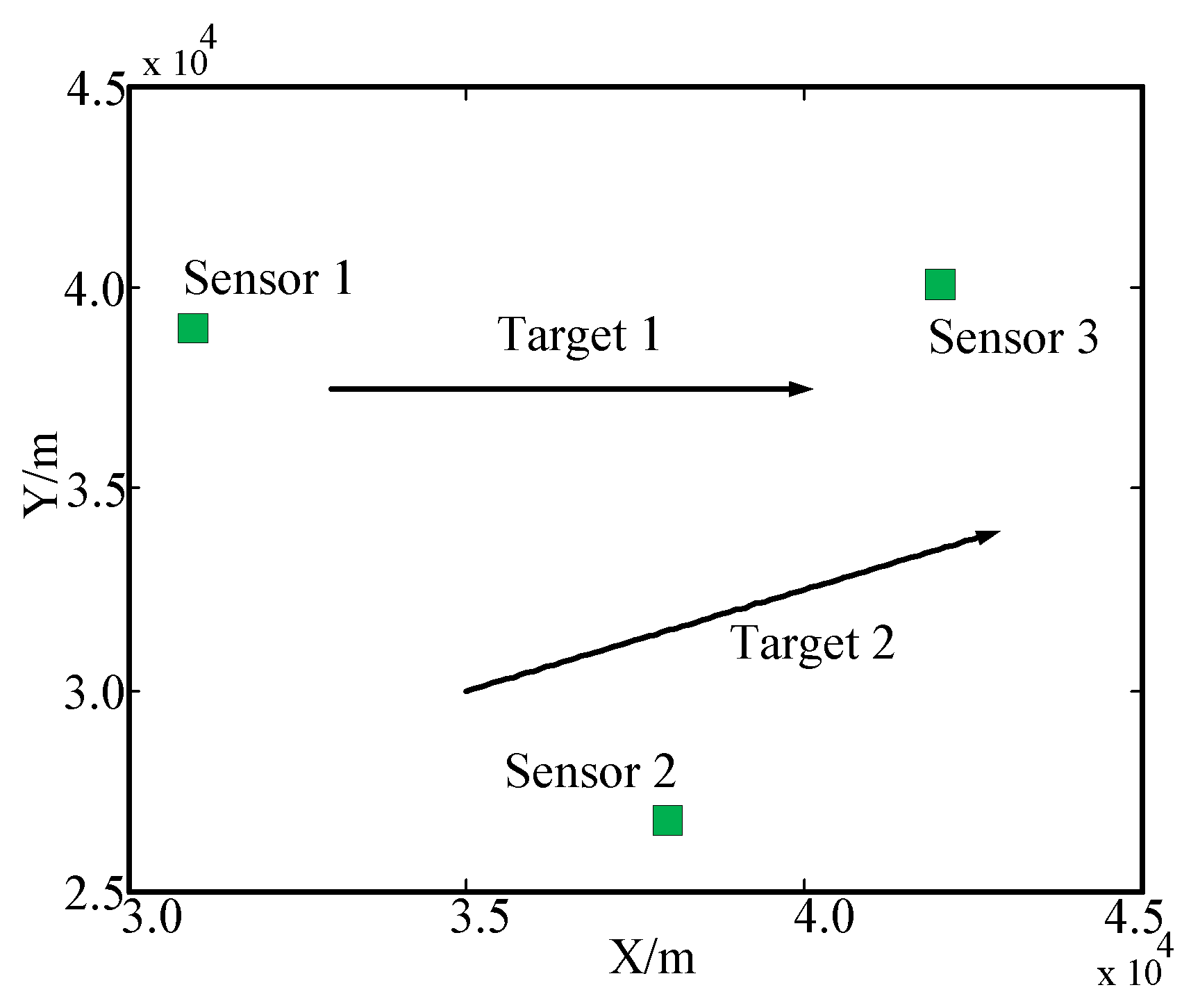
In this scenario, the number of targets is assumed to be M = 2 and the target motion model is a constant velocity model. Without loss of generality, the initial positions of 2 targets are (33 km, 37.5 km) and (35 km, 30 km), respectively, and the other experimental parameters are set up as follows

$${\mathit{x}}_0^1={\left[\begin{array}{cccc}33000& 90& 37500& 0\end{array}\right]}^{\mathrm{T}}\mathrm{m},x_0^2={\left[\begin{array}{cccc}35000& 100& 30000& 50\end{array}\right]}^{\mathrm{T}}\mathrm{m}$$

$${\mathit{P}}_0^1={\mathit{P}}_0^2=diag(1000,25,1000,25)\mathrm{m}$$

$$\mathit{F}=\left[\begin{array}{cccc}1& T& 0& 0\\ 0& 1& 0& 0\\ 0& 0& 1& T\\ 0& 0& 0& 1\end{array}\right],\mathsf{\Gamma }=\left[\begin{array}{cc}\begin{array}{c}{T}^2/2\\ T\\ 0\\ 0\end{array}& \begin{array}{c}0\\ 0\\ T^2/2\\ T\end{array}\end{array}\right],\begin{array}{c}{\mathit{Q}}^1=\left[\begin{array}{cc}20& 0\\ 0& 20\end{array}\right]\\ {\mathit{Q}}^2=\left[\begin{array}{cc}20& 0\\ 0& 20\end{array}\right]\end{array}$$

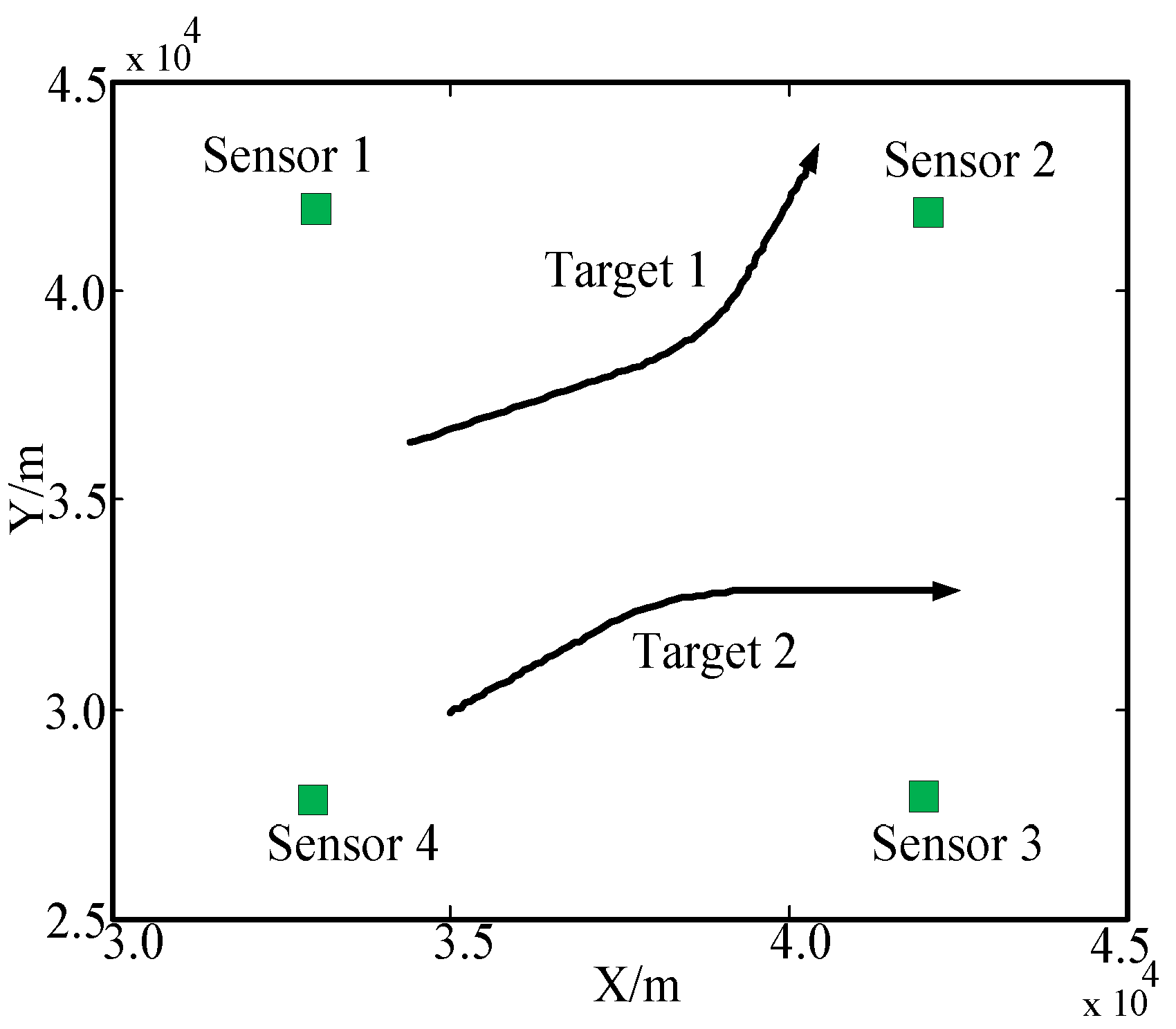
where ${\mathit{Q}}^1,{\mathit{Q}}^2$ are covariance matrices of state transition noise. The number of sensors is assumed to be $N=3$, which are placed at (31 km, 39 km), (38 km, 27 km), and (42 km, 40 km), respectively. The covariance matrices of measurement noise of the 3 sensors are set up as follows. It is shown that the tracking ability of sensor 1 and 3 is better than sensor 2. The sensor positions and target trajectories in the battlefield are shown in Figure 8.

$${\mathit{R}}^1=diag([{50}^2,{0.02}^2]),{\mathit{R}}^2=diag([{100}^2,{0.02}^2]),{\mathit{R}}^3=diag([{50}^2,{0.02}^2])$$

Meanwhile, to prove the advantages of our proposed IPF based sensor scheduling policy (IPFSP), the other two scheduling policies are used for comparison experiments. (1) Stationary scheduling policy (SSP): In this method, the sensor is fixed to track the specific target. (2) Bhattacharyya distance based scheduling policy (BDSP): It is proposed in [13] that the method can keep a small intercept probability of the whole sensor network by maximizing Bhattacharyya distance. Without loss of generality, sensor 1 is used to track target 1 and sensor 3 is used to track target 2 in SSP. Additionally, sensor 1 is used to track target 1 and sensor 2 is used to track target 2 at the beginning in BDSP and IPFSSP.

The number of Monte Carlo experiments is 150, and experimental results are shown in Figure 9, Figure 10, Figure 11 and Figure 12.

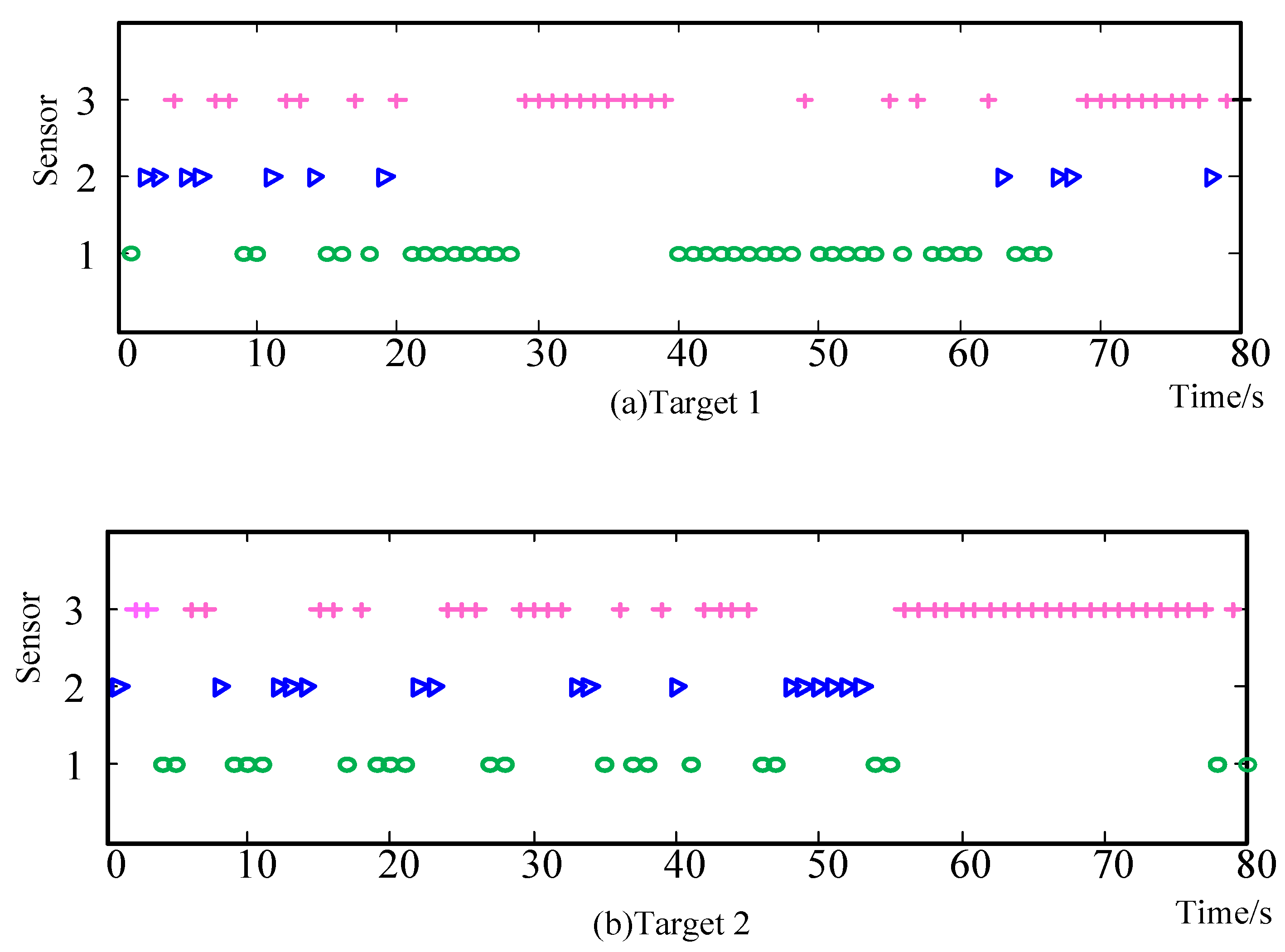
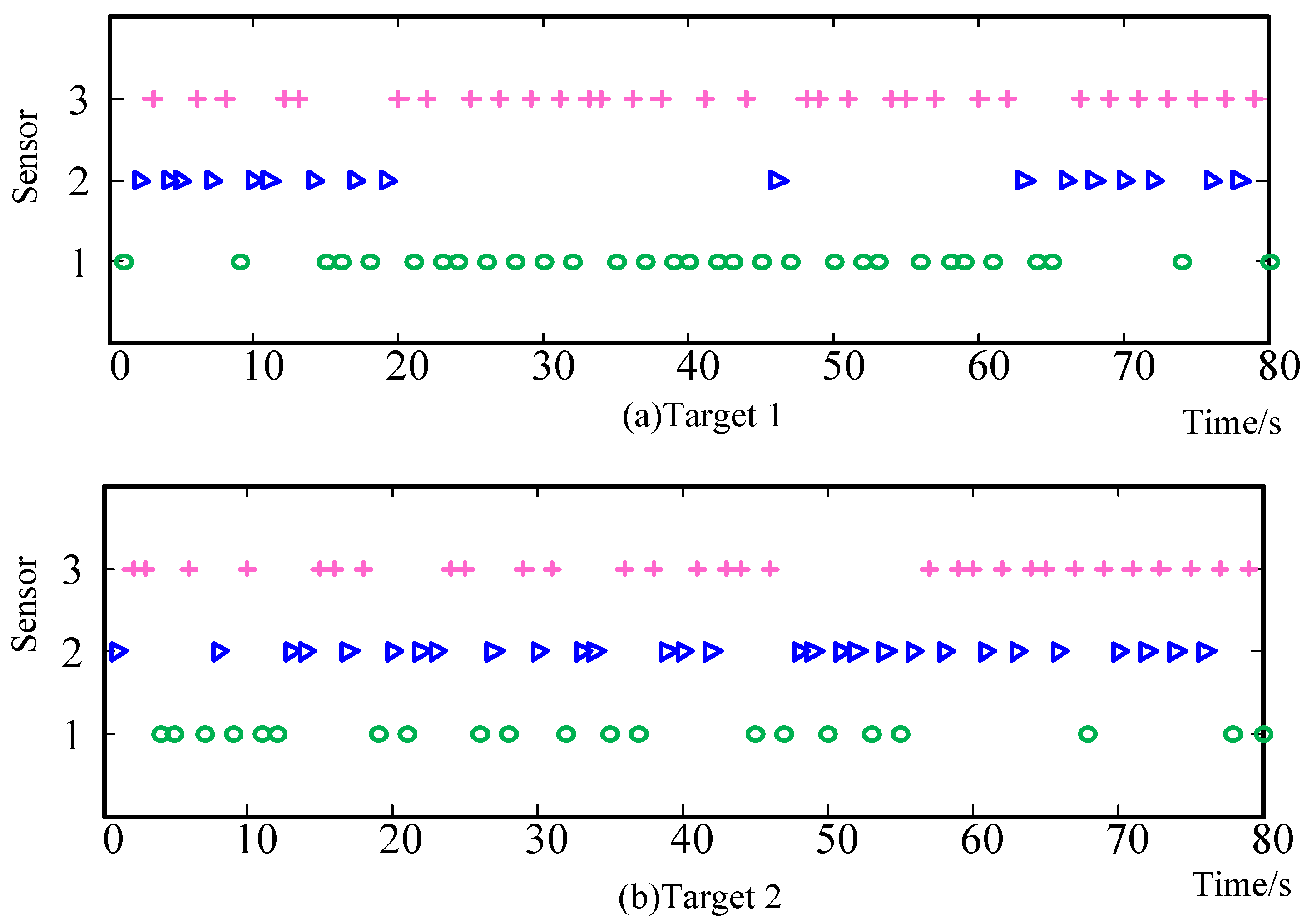
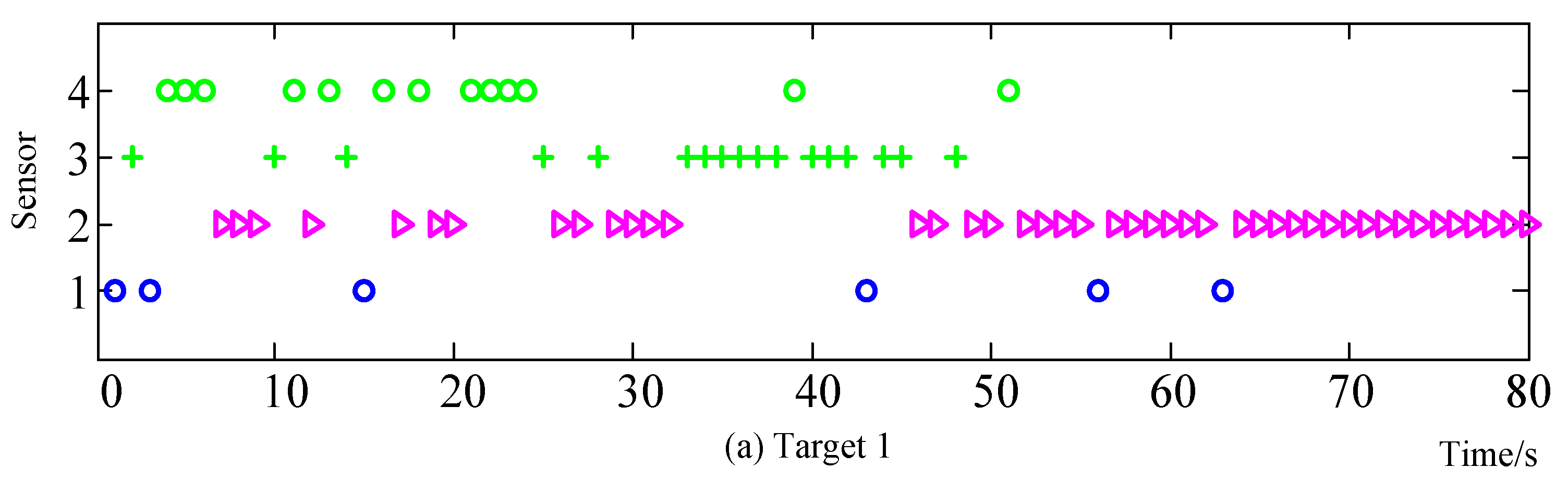
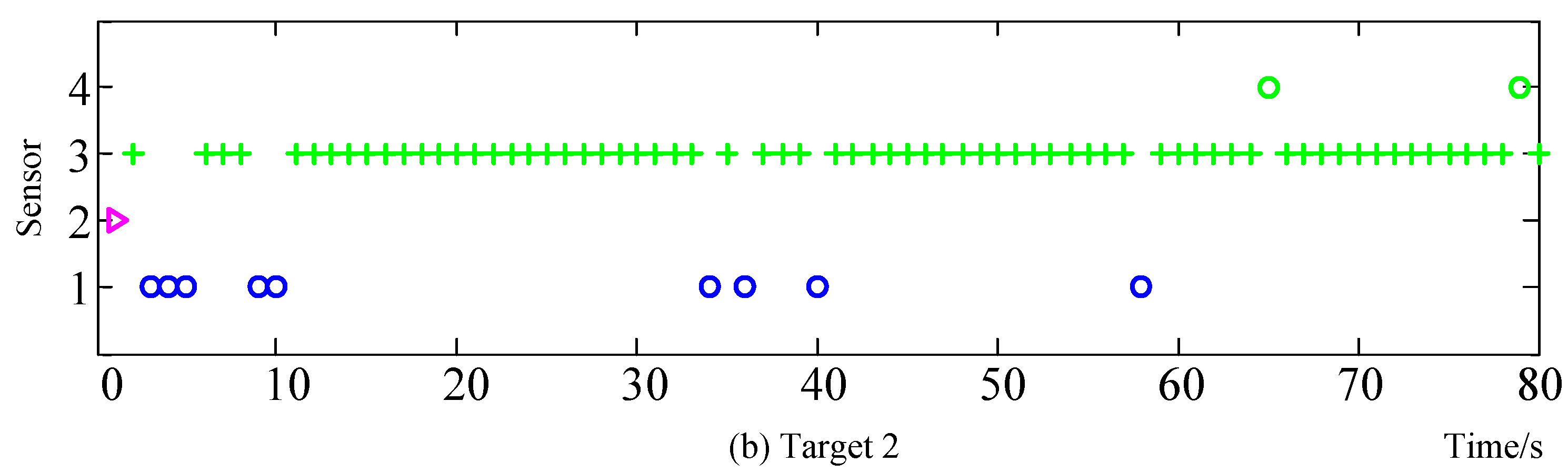
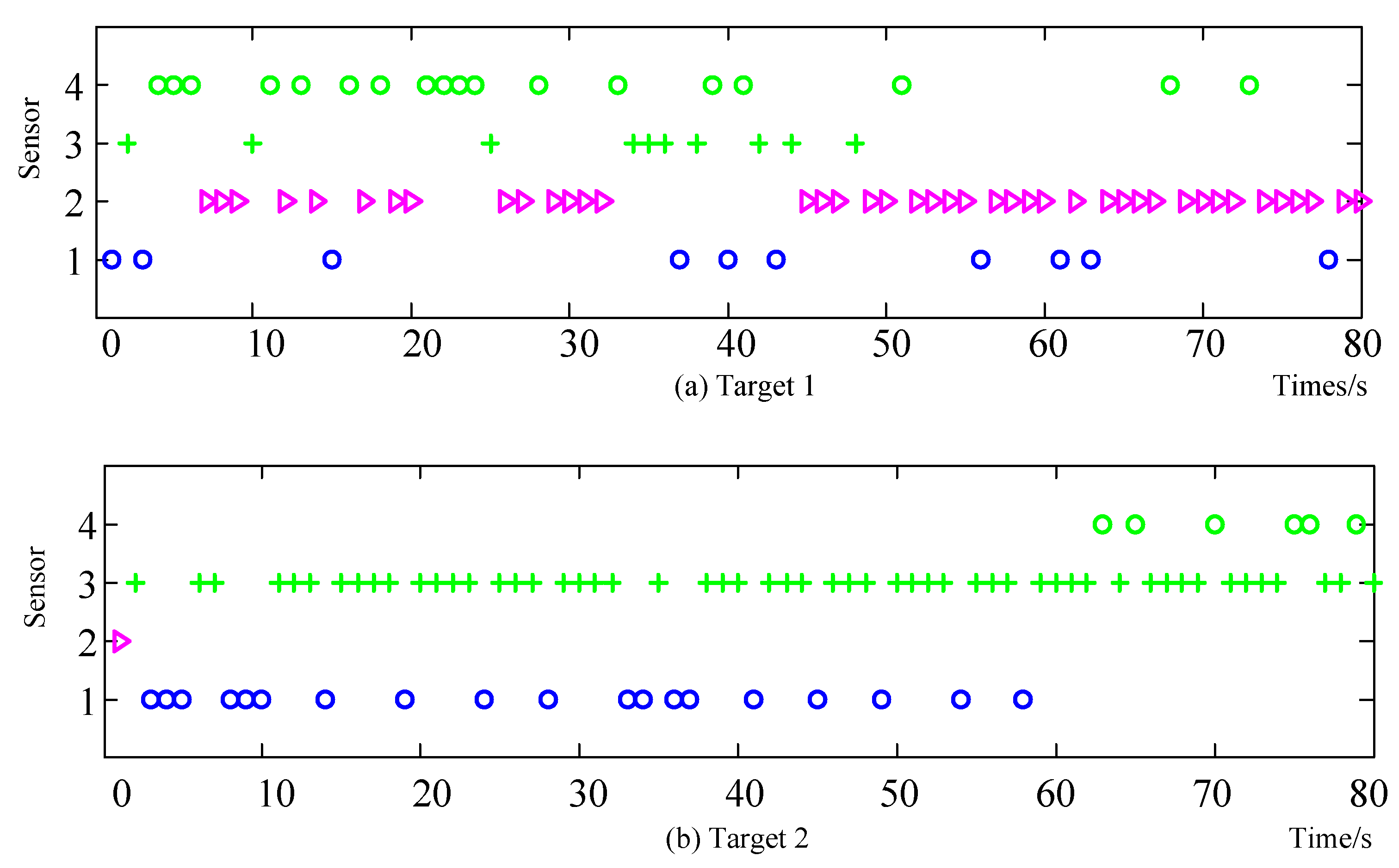
The sensor selection sequences obtained by BDSP and IPFSP methods for the 2 targets are shown in Figure 9 and Figure 10. The horizontal coordinate is the simulation time, and the vertical coordinate is the sensor number. It can be seen that the proposed IPFSP model can realize reasonable selection of sensors for tracking target. Moreover, the sensor switching frequency of IPFSP method is greater than BDSP method. The reason is that the sensor cannot track a target for a long time due to the limitation of IPF. In this way, the intercepted probability of sensors by enemies will be reduced greatly.

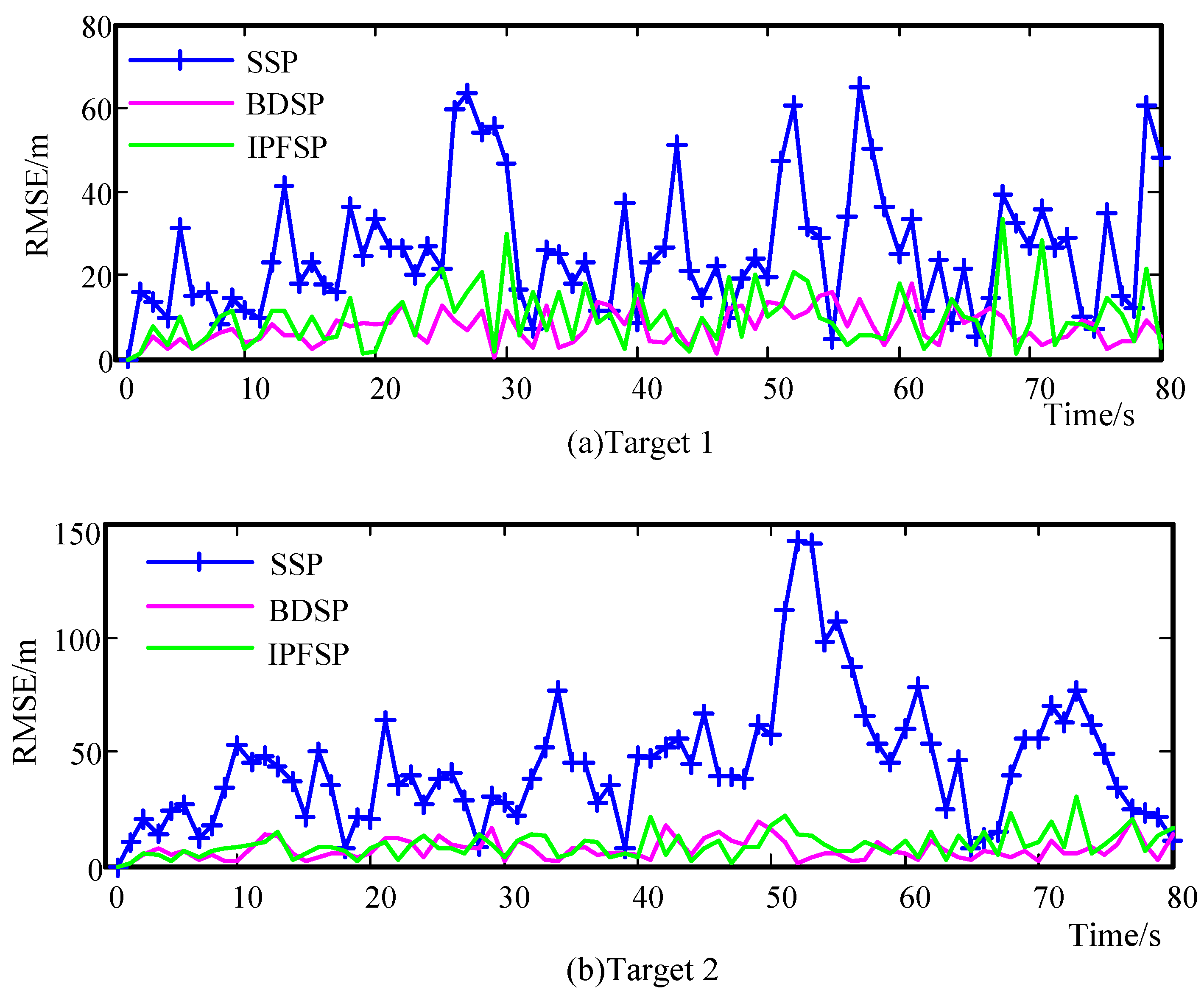
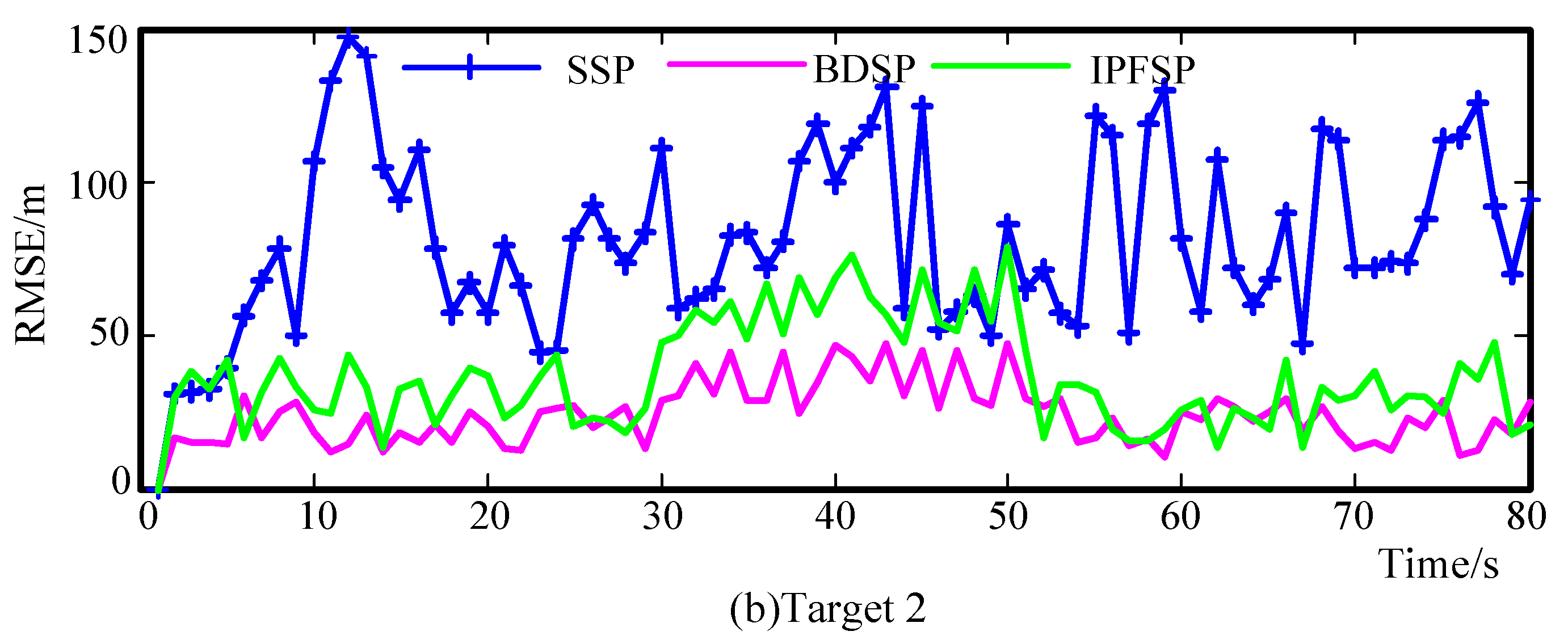
Figure 11 shows the root mean-square error (RMSE) curves of the target position under the SSP, MSP, and BDSP methods. We can see that the tracking accuracy under BDSP and IPFSP are better than that under SSP. The RMSE averages of target 1 under SSP, BDSP, and IPFSP are 34.27 m, 7.03 m and 8.56 m, respectively. It proves that although the sensor is frequently selected and switched in IPFSP method during the tracking process, the tracking accuracy of targets is still at a high level compared with SSP method.

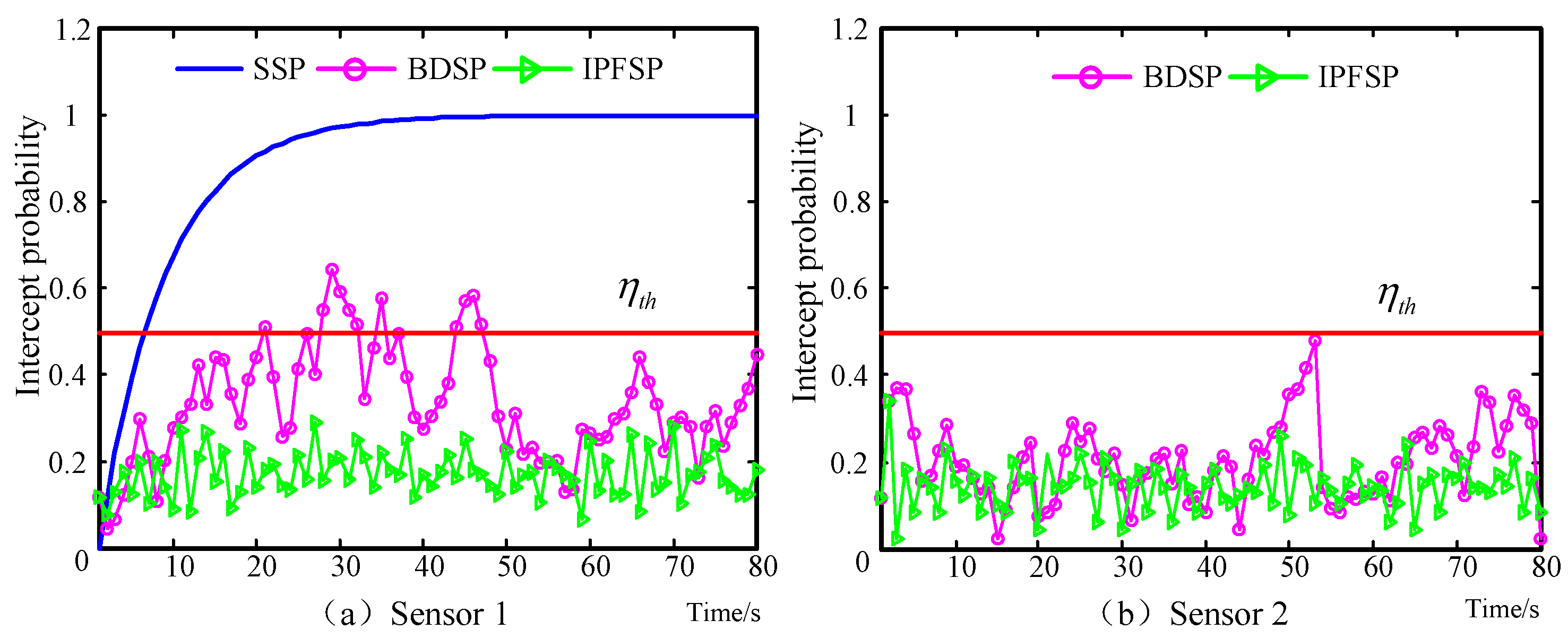
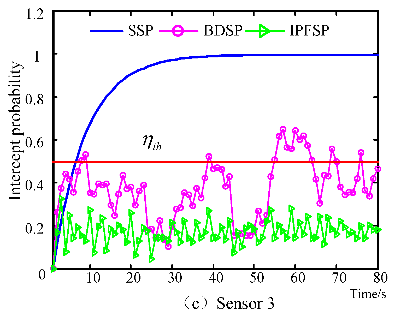
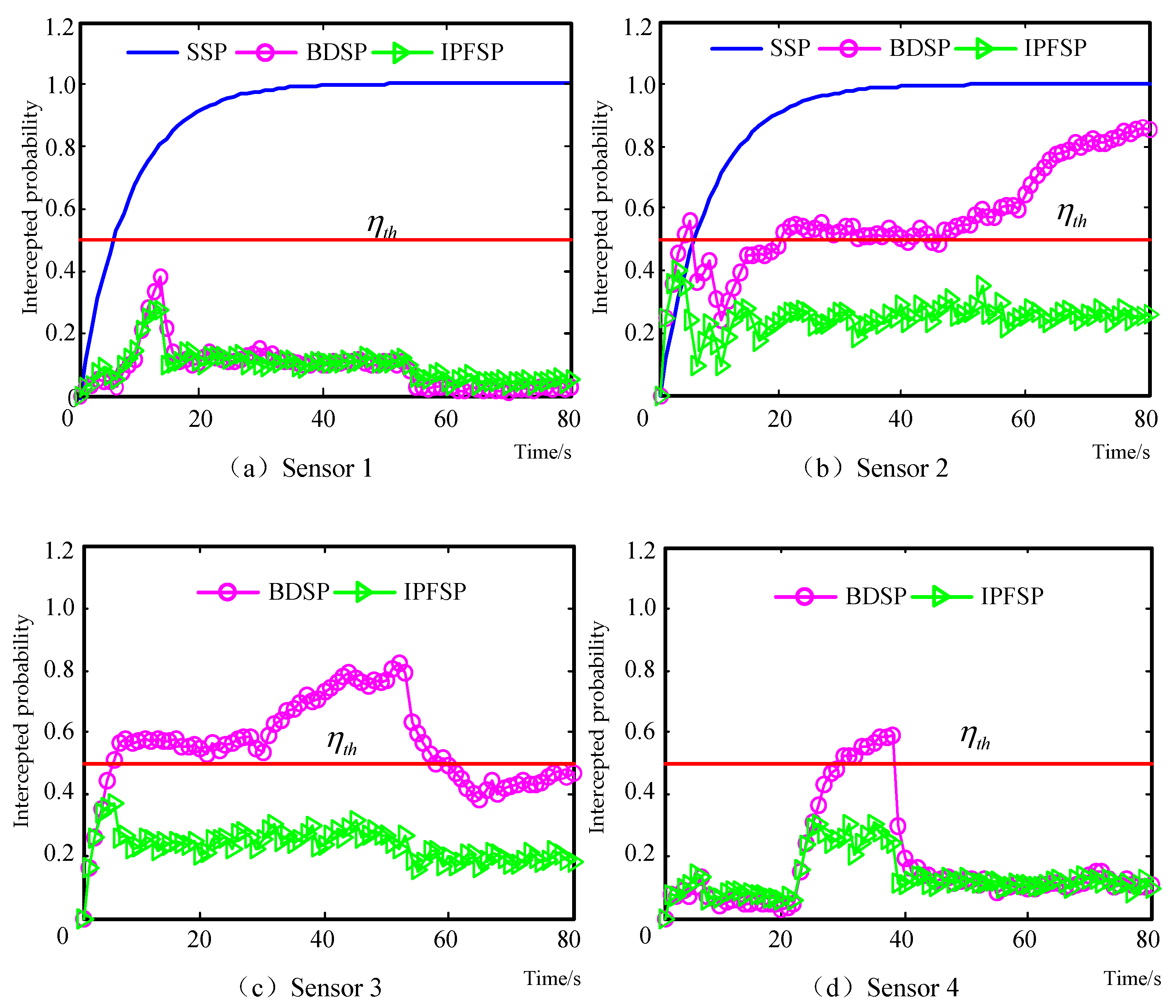
Figure 12 shows the variation curves of sensor intercepted probability under different scheduling policies. The average intercepted probabilities of the sensor system under SSP, BDSP, and IPFSP are 0.60, 0.35 and 0.16, respectively. Besides, the intercepted probability of SSP increases over the simulation period, which is more than the security threshold ${\eta }_{th}$ at most time. The intercepted probability of BDSP sometimes goes beyond the security threshold ${\eta }_{th}$. On the contrary, the IPFSP can effectively control the intercepted probability of the 3 sensors within the security threshold ${\eta }_{th}$ the whole time, which shows the advancement of the proposed sensor scheduling method.

6.2. Scenario 2

In this scenario, the numbers of sensors and targets are set up in order to analyze the effectiveness of the proposed model and solving algorithm for large-scale tracking scenarios. The number of targets is assumed to be M = 4 and the target motion model is also the CV model. The initial states of 4 targets are set up as in Equation (26), and the other parameters are the same as in Scenario 1.

$$\{\begin{array}{l}{\mathit{x}}_0^1={\left[\begin{array}{cccc}37300& -80& 40000& -60\end{array}\right]}^{\mathrm{T}}\mathrm{m}\\ {\mathit{x}}_0^2={\left[\begin{array}{cccc}37000& 60& 29000& 70\end{array}\right]}^{\mathrm{T}}\mathrm{m}\\ {\mathit{x}}_0^3={\left[\begin{array}{cccc}43000& -60& 35000& 80\end{array}\right]}^{\mathrm{T}}\mathrm{m}\\ {\mathit{x}}_0^4={\left[\begin{array}{cccc}32000& 80& 30000& -60\end{array}\right]}^{\mathrm{T}}\mathrm{m}\end{array}$$

(26)

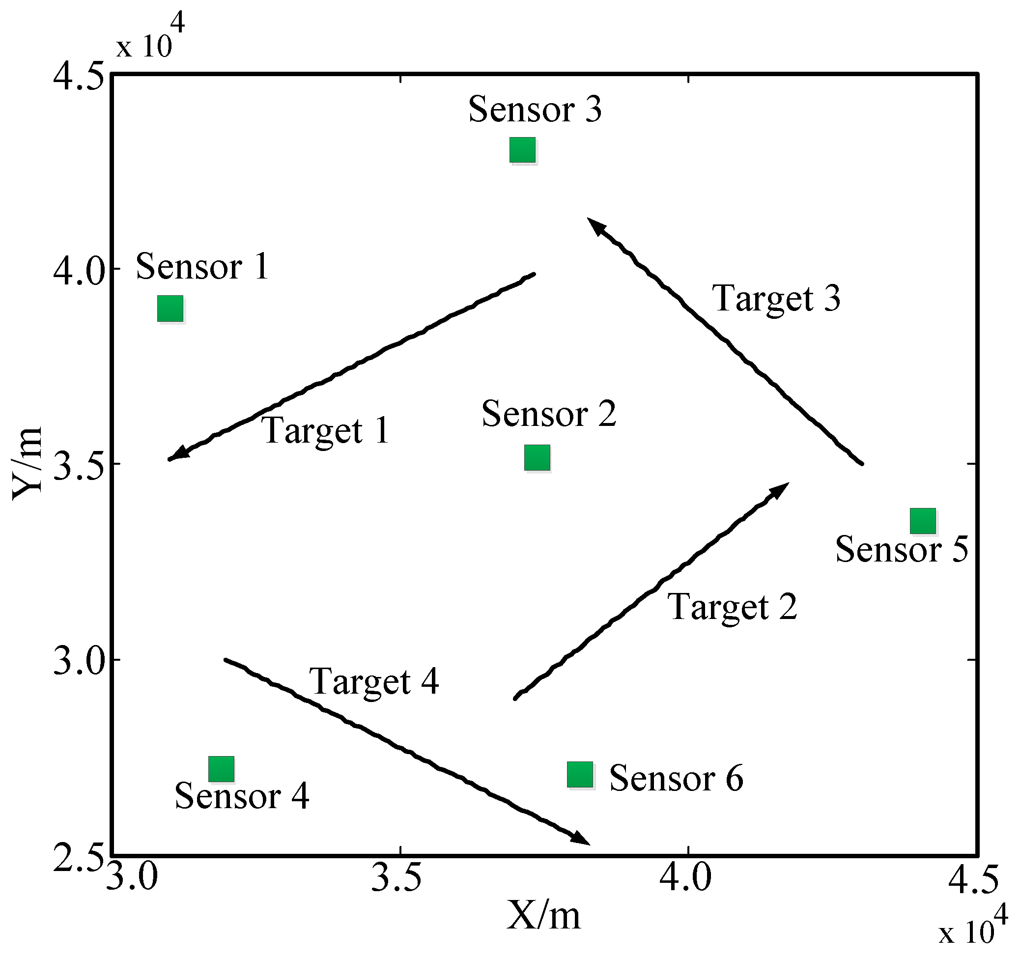
In addition, the sensor numbers are assumed to be N = 6, which are placed at (31 km, 39 km), (37.5 km, 35 km), (37 km, 43 km), (32 km, 27 km), (44 km, 33 km), and (38 km, 27 km), respectively, and the measurement covariance matrices of the 6 sensors are set up as ${\mathit{R}}^1={\mathit{R}}^2={\mathit{R}}^3={\mathit{R}}^4={\mathit{R}}^5={\mathit{R}}^6=$ $diag([{50}^2,{0.02}^2])$. In SSP method and at the beginning of BDSP and IPFSP methods, sensor 1, sensor 2, sensor 3, and sensor 4 are used to track target 1, target 2, target 3, and target 4, respectively. Sensor positions and target trajectories in the battlefield are shown in Figure 13.

Furthermore, the number of Monte Carlo experiments is 150, and the simulation results are shown in Figure 14, Figure 15, Figure 16 and Figure 17.

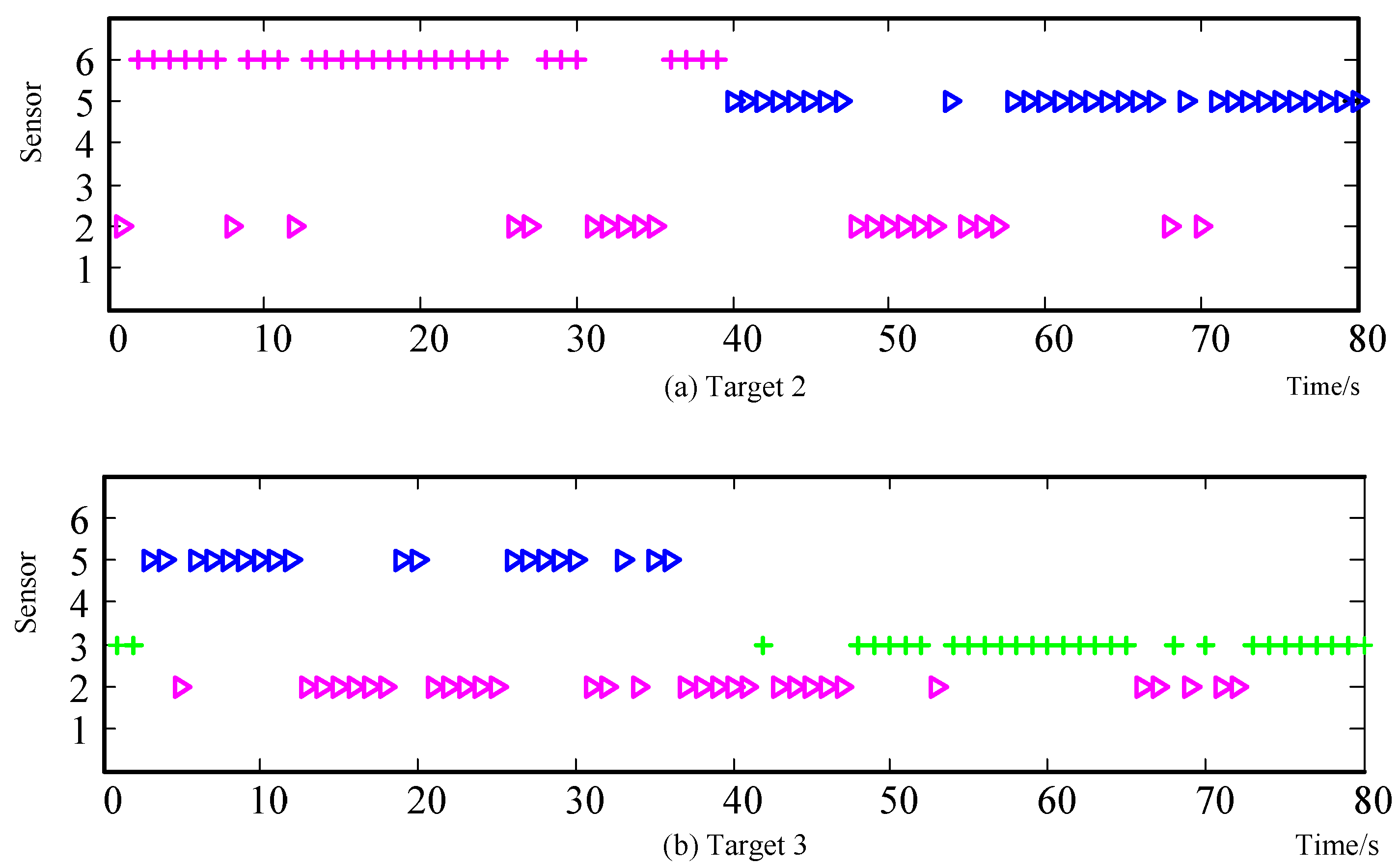
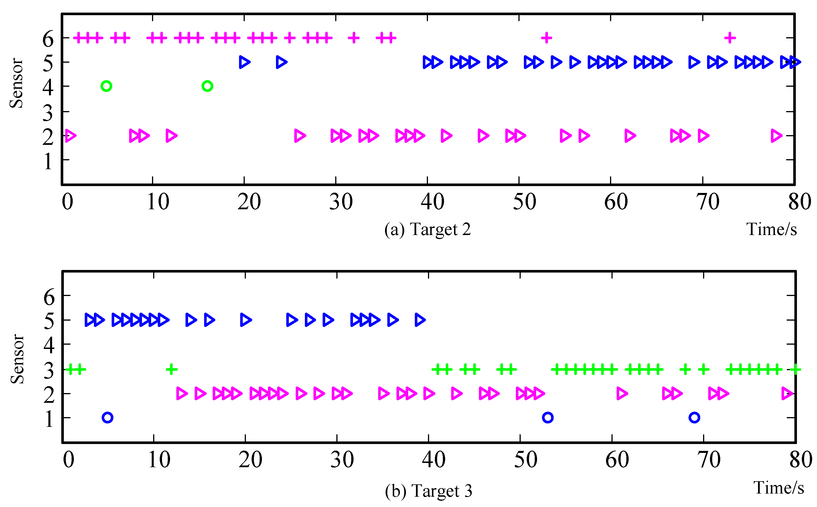
Figure 14 and Figure 15 show the sensor selected sequence for target 2 and target 3 by BDSP and IPFSP methods, respectively. It can be seen that for sensor and target scheduling problems, the proposed method can also realize the effective scheduling of sensors to track targets in this scenario. Compared with BDSP, the sensor switching frequency of IPFSP is also greater than BDSP method, which is due to the limitation of novel IPF. In this way, the intercept probability of the sensors will be reduced greatly, which we can see in Figure 16. The results are the same for target 1 and target 4.

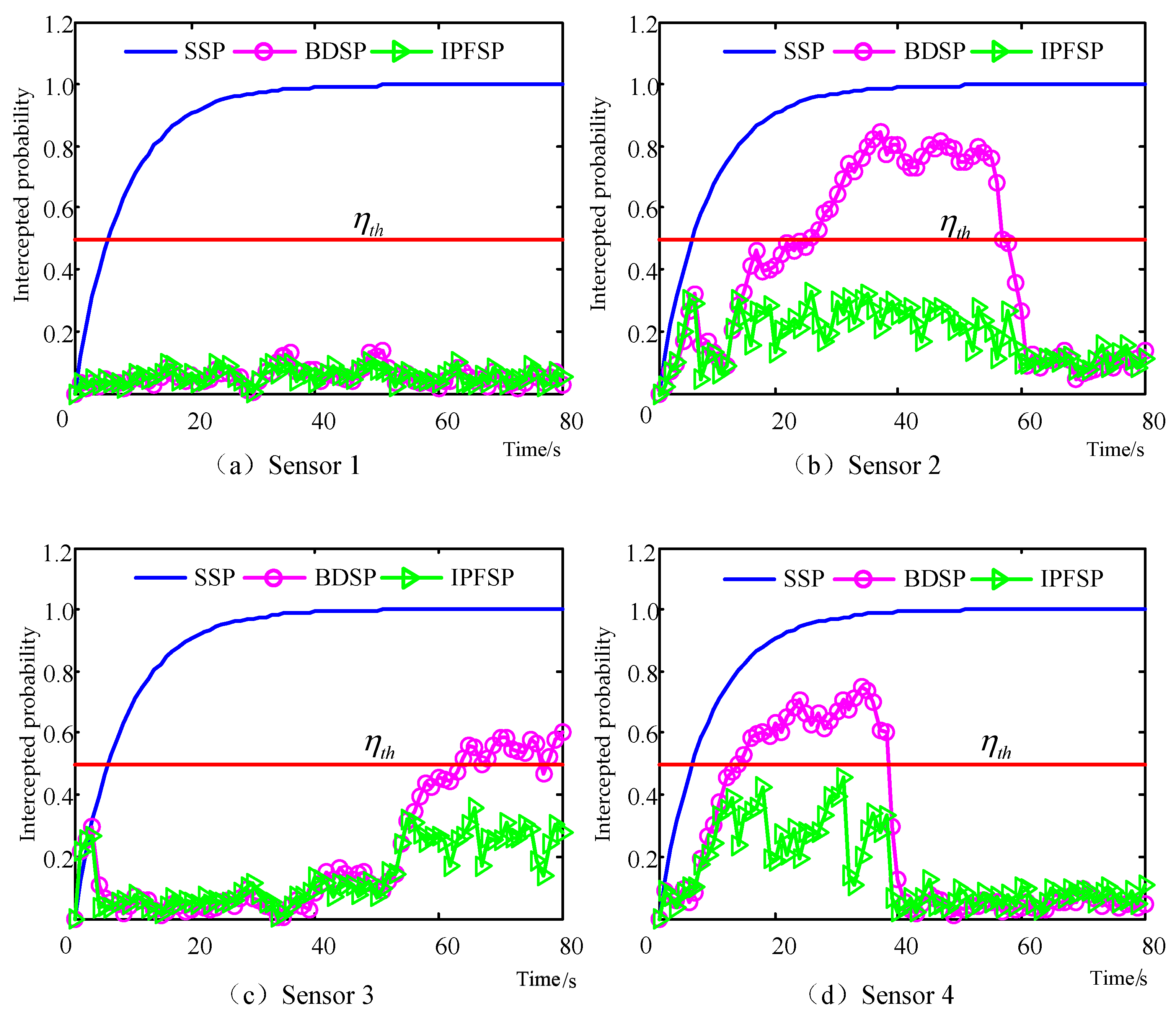
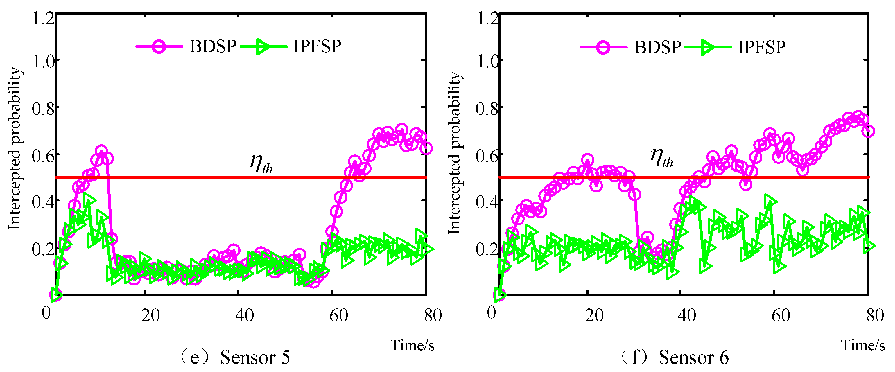
Figure 16 shows the variation curves of sensor intercept probability under different scheduling policies. The average intercept probabilities of the sensor system under SSP, BDSP, and IPFSP are 0.60, 0.37, and 0.15, respectively. Moreover, it can be seen from Figure 16 that when using SSP method, the intercept probabilities of sensor 1, 2, 3, and 4 are more than the security threshold at most times. When using BDSP method, the intercept probability of all sensors will be more than the security threshold sometimes. On the contrary, the proposed IPFSP method can control the intercept probability of all sensors within the security threshold ${\eta }_{th}$. It can be concluded that the proposed IPFSP method can effectively improve sensor battlefield survivability for different target tracking scenarios.

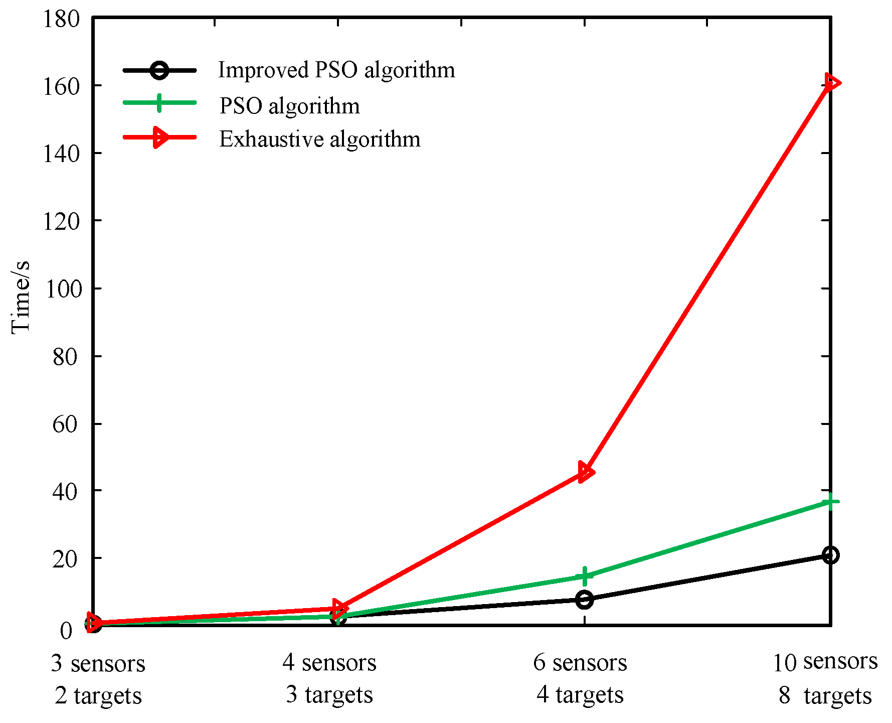
Figure 17 shows the running time of an experiment under different solution algorithms. Compared with the exhaustive search algorithm and traditional PSO algorithm, some experiments with different numbers of sensors and targets are carried out to verify the advancement of the proposed solution algorithm. We can see that with the increase of sensor and target numbers, the running time of the exhaustive search algorithm will grow rapidly, which cannot match the real-time requirement. However, the running time of the proposed algorithm in this paper is always less. Besides, Figure 16 shows that the running time of the improved PSO algorithm is less than that of the traditional PSO algorithm, which proves the effectiveness of the improvement strategy. Compared with the traditional PSO algorithm, when the sensor number is 4 and target number is 3, the running time is reduced by 14.87%. When the sensor number is 6 and target number is 4, it is reduced by 30.32%. When the sensor number is 10 and target number is 8, it is reduced by 47.51%. It can be concluded that the more complex the problem is, the more time will be saved by the proposed solution algorithm.

6.3. Scenario 3

In this scenario, two maneuverable targets are considered to verify the applicability of the proposed sensor scheduling method for the problem of maneuverable target tracking. As is shown in Figure 18, the initial position of target 1 is (34 km, 36 km), and target 1 turns left with $\omega =-2\mathrm{rad}/\mathrm{s}$ during 30 s~50 s and maintains uniform motion during the other time. The initial positions of target 2 is (35 km, 30 km), and target 1 turns right with $\omega =2\mathrm{rad}/\mathrm{s}$ during 30 s~50 s and maintains uniform motion during the other time. The initial states of 2 targets are set up as ${\mathit{x}}_0^1={\left[\begin{array}{cccc}34000& 110& 36000& 60\end{array}\right]}^{\mathrm{T}}\mathrm{m}$, ${\mathit{x}}_0^2={\left[\begin{array}{cccc}35000& 80& 30000& 70\end{array}\right]}^{\mathrm{T}}\mathrm{m}$. The other parameters are the same as in Scenario 1.

There are 4 sensors which are placed at (33 km, 28 km), (33 km, 42 km), (42 km, 28 km), and (42 km, 42 km). The measurement covariance matrices of the 4 sensors are set up as ${\mathit{R}}^1={\mathit{R}}^2={\mathit{R}}^3={\mathit{R}}^4=$ $diag([{50}^2,{0.02}^2])$. In the SSP method and at the beginning of the BDSP and IPFSP methods, sensor 1 and sensor 2 are used to track target 1 and target 2, respectively. The number of Monte Carlo experiments is 150, and the simulation results are shown in Figure 19, Figure 20, Figure 21 and Figure 22.

Figure 19 and Figure 20 show the sensor selected sequence for the two maneuverable targets by BDSP and IPFSP methods, respectively. Obviously, in this scenario, the proposed method can also realize the effective scheduling of sensors to track maneuverable targets, which proves the wide applicability of the proposed sensor scheduling method.

Figure 21 shows the root mean-square error (RMSE) curves of the target position under the SSP, BDSP, and IPFSP methods in this scenario. The RMSE averages of target 1 under SSP, BDSP, and IPFSP are 74.20 m, 20.56 m, and 32.42 m, respectively. Compared with the uniform moving targets in scenario 1 and scenario 2, the tracking error under IPFSP method is still less than that under SSP method, but it is greater than that under BDSP method. Therefore, it can be concluded that for maneuvering targets, the target tracking accuracy of the proposed method will be declined.

Figure 22 shows the variation curves of sensor intercept probability under different scheduling policies in this scenario. The average intercept probabilities of the sensor system under SSP, BDSP, and IPFSP are 0. 49, 0.36, and 0.16, respectively. It can be seen from Figure 22 that the proposed IPFSP method can also control the intercept probability of all sensors within the security threshold ${\eta }_{th}$. The intercept probability of the other two methods will be more than the security threshold at most times. It is proved that the proposed method can perform well for maneuvering target tracking scenarios.

7. Conclusions

In this paper, in order to reduce the intercept risk and maintain the target tracking accuracy of radar sensor networks, an active multi-sensor scheduling method based on PCRLB and a novel IPF is proposed. Firstly, the target moving model and sensor measurement model are introduced. Then, the calculation methods of PCRLB for uniform moving targets and maneuvering targets are presented. Next, to accurately assess the intercepted risk of sensors, a novel intercept probability factor is given based on multiple window functions. Simulation results show that the proposed method can reasonably evaluate the intercept risk of all sensors in the future for different multi-target tracking scenarios. The minimum average intercept probability of the sensor network system is only 0.15 with better target tracking accuracy, which is much better than the existing SSP and BDSP methods. In addition, in order to quickly get the optimal scheduling actions, a fast solution algorithm based on the improved PSO algorithm is proposed. When the sensor number is 6 and target number is 5, the running times can be reduced by 30.32%, and more time will be saved by the proposed solution algorithm when the sensor and target numbers increase. For the other optimization problems, the improved PSO algorithm also has certain application value.

In the future, with combat situations becoming more complex and more diverse, sensor scheduling models aiming at an individual combat mission seem unlikely to meet combat requirements. The multi-task sensor scheduling problem will need to be considered, and further study will need to be conducted on combinations of target detection, target tracking, and target recognition. Besides, in actual situations, different targets have different threat levels, so the problem of target priority assessment will also need to be studied with the sensor scheduling problem.

References

- Akyildiz, I.F.; Su, W.; Sankarasubramaniam, Y.; Cayirci, E. A survey on sensor networks. IEEE Commun. Mag. 2002, 40, 102–105. [Google Scholar] [CrossRef]
- Salvagnini, P.; Pernici, F.; Cristani, M.; Lisanti, G.; Del Bimbo, A.; Murino, V. Non-myopic information theoretic sensor management of a single pan-tilt-zoom camera for multiple object detection and tracking. Comput. Vis. Image Underst. 2015, 134, 74–88. [Google Scholar] [CrossRef]
- Zhang, Z.N.; Shan, G.L. Non-myopic sensor scheduling to track multiple reactive targets. Signal Process. IET 2015, 9, 37–47. [Google Scholar] [CrossRef]
- Gupta, R.; Sultania, K.; Singh, P.; Gupta, A. Security for wireless sensor networks in military operations. In Proceedings of the IEEE Fourth International Conference on Computing, Communications and Networking Technologies, Tiruchengode, India, 4–6 July 2013; pp. 1–6. [Google Scholar]
- Collotta, M.; Bello, L.L.; Pau, G. A novel approach for dynamic traffic lights management based on wireless sensor networks and multiple fuzzy logic controllers. Expert Syst. Appl. 2015, 42, 5403–5415. [Google Scholar] [CrossRef]
- Wu, H.; Shi, Z.Y.; Shen, W.D.; Wang, J.S.; Wang, W.Z. Design of LPI radar waveform based on chaos theory. Comput. Eng. Appl. 2017, 53, 241–244. [Google Scholar]
- Deng, H. Waveform design for MIMO radar with low probability of intercept (LPI) property. In Proceedings of the IEEE International Symposium on Antennas and Propagation, Spokane, WA, USA, 3–8 July 2011; pp. 305–308. [Google Scholar]
- Chen, J.; Wang, F.; Zhou, J. Information Content Based Optimal Radar Waveform Design: LPI’s Purpose. Entropy 2017, 19, 210. [Google Scholar] [CrossRef]
- Angley, D.; Ristic, B.; Suvorova, S.; Moran, B.; Fletcher, F.; Gaetjens, H.; Simakov, S. Non-myopic sensor scheduling for multi-static sonobuoy fields. IET Radar Sonar Navig. 2017, 11, 1770–1775. [Google Scholar] [CrossRef]
- Shi, C.; Wang, F.; Salous, S.; Zhou, J. Optimal Power Allocation Strategy in a Joint Bistatic Radar and Communication System Based on Low Probability of Intercept. Sensors 2017, 17, 2731. [Google Scholar] [CrossRef]
- Rim, J.W.; Jung, K.H.; Koh, I.S.; Baek, C.; Lee, S.; Choi, S.H. Simulation of Dynamic EADs Jamming Performance against Tracking Radar in Presence of Airborne Platform. Int. J. Aeronaut. Space Sci. 2015, 16, 475–483. [Google Scholar] [CrossRef] [Green Version]
- She, J.; Zhou, J.; Wang, F.; Li, H. LPI optimization framework for radar network based on Minimum mean-square error estimation. Entropy 2017, 19, 397. [Google Scholar] [CrossRef]
- Shi, C.; Wang, F.; Sellathurai, M.; Zhou, J. LPI optimization framework for target tracking in radar network architectures using information theoretic criteria. Int. J. Antennas Propag. 2014, 2014. [Google Scholar] [CrossRef]
- Zhang, Z.; Zhu, J.; Salous, S. A novel dwelling time design method for low probability of intercept in a complex radar network. Int. J. Des. Nat. Ecodyn. 2015, 10, 309–318. [Google Scholar] [CrossRef]
- Krishnamurthy, V. Emission management for low probability intercept sensors in network centric warfare. IEEE Trans. Aerosp. Electron. Syst. 2005, 41, 133–151. [Google Scholar] [CrossRef]
- Shan, G.L.; Zhang, Z.N. Non-myopic sensor scheduling for low radiation risk tracking using mixed POMDP. Trans. Inst. Meas. Control 2015, 39. [Google Scholar] [CrossRef]
- Tichavsky, P.; Muravchik, C.H.; Nehorai, A. Posterior Cramer-Rao bounds for discrete-time nonlinear filtering. IEEE Trans.Signal Process. 1998, 46, 1386–1396. [Google Scholar] [CrossRef] [Green Version]
- Stein, S.; Johansen, D. A Statistical Description of Coincidences among Random Pulse Trains. Proc. IRE 2007, 46, 827–830. [Google Scholar] [CrossRef]
- Self, A.G.; Smith, B.G. Intercept time and its prediction. IEE Proc. F Commun. Radar Signal Process. 2008, 132, 215–220. [Google Scholar] [CrossRef]
- Masdari, M.; Salehi, F.; Jalali, M.; Bidaki, M. A Survey of PSO-Based Scheduling Algorithms in Cloud Computing. J. Netw. Syst. Manag. 2017, 25, 122–158. [Google Scholar] [CrossRef]
- Geng, J.C.; Cui, Z.; Gu, X.S. Scatter search based particle swarm optimization algorithm for earliness/tardiness flow shop scheduling with uncertainty. Int. J. Autom. Comput. 2016, 13, 285–295. [Google Scholar] [CrossRef]
- Trelea, I.C. The particle swarm optimization algorithm: Convergence analysis and parameter selection. Inf. Process. Lett. 2003, 85, 317–325. [Google Scholar] [CrossRef]
- Naidu, Y.R.; Ojha, A.K. Solving Multi-objective Optimization Problems Using Hybrid Cooperative Invasive Weed Optimization With Multiple Populations. IEEE Trans. Syst. Man Cybern. Syst. 2016, 48, 821–832. [Google Scholar] [CrossRef]
Figure 1.
Description of sensor scheduling problem.
Figure 2.
Basic window functions and the time overlap of them.
Figure 3.
Change curves of IPF with time.
Figure 4.
Change curves of IPF for different target numbers.
Figure 5.
Process of multi-sensor scheduling at time k.
Figure 6.
Multi-population cooperation searching strategy.
Figure 7.
An example of discretization and legalization processes.
Figure 8.
Sensor positions and target trajectories.
Figure 9.
Sensor selected sequences obtained by BDSP. (a) Target 1; (b) Target 2.
Figure 10.
Sensor selected sequences obtained by IPFSP. (a) Target 1; (b) Target 2.
Figure 11.
RMSE of the target position under different scheduling policies. (a) Target 1; (b) Target 2.
Figure 12.
Sensor intercepted probability under different scheduling policies. (a) Sensor 1; (b) Sensor 2; (c) Sensor 3.
Figure 13.
Figure 14.
Sensor selected sequences obtained by BDSP. (a) Target 2; (b)Target 3.
Figure 15.
Sensor selected sequences obtained by IPFSP. (a) Target 2; (b) Target 3.
Figure 16.
Sensor intercept probability under different scheduling policies. (a) Sensor 1; (b) Sensor 2; (c) Sensor 3; (d) Sensor 4; (e) Sensor 5; (f) Sensor 6.
Figure 17.
Running time of an experiment under different solution algorithms.
Figure 18.
Figure 19.
Figure 20.
Figure 21.
RMSE of target position under different scheduling policies. (a) Target 1; (b) Target 2.
Figure 22.
Sensor intercept probability under different scheduling policies. (a) Sensor 1; (b) Sensor 2; (c) Sensor 3; (d) Sensor 4.
© 2019 by the authors. Licensee MDPI, Basel, Switzerland. This article is an open access article distributed under the terms and conditions of the Creative Commons Attribution (CC BY) license (http://creativecommons.org/licenses/by/4.0/).
Share and Cite
MDPI and ACS Style
Xu, G.; Pang, C.; Duan, X.; Shan, G. Multi-Sensor Optimization Scheduling for Target Tracking Based on PCRLB and a Novel Intercept Probability Factor. Electronics 2019, 8, 140. https://doi.org/10.3390/electronics8020140
AMA Style
Xu G, Pang C, Duan X, Shan G. Multi-Sensor Optimization Scheduling for Target Tracking Based on PCRLB and a Novel Intercept Probability Factor. Electronics. 2019; 8(2):140. https://doi.org/10.3390/electronics8020140
Chicago/Turabian StyleXu, Gongguo, Ce Pang, Xiusheng Duan, and Ganlin Shan. 2019. "Multi-Sensor Optimization Scheduling for Target Tracking Based on PCRLB and a Novel Intercept Probability Factor" Electronics 8, no. 2: 140. https://doi.org/10.3390/electronics8020140
Note that from the first issue of 2016, this journal uses article numbers instead of page numbers. See further details here.