Through-Wall Single and Multiple Target Imaging Using MIMO Radar


1
The Pennsylvania State University, University Park, PA 16802, USA
2
U.S. Army RDECOM CERDEC, Aberdeen Proving Ground, Aberdeen, MD 21005, USA
*
Author to whom correspondence should be addressed.
Electronics 2017, 6(4), 70; https://doi.org/10.3390/electronics6040070
Submission received: 21 August 2017
/
Revised: 13 September 2017
/
Accepted: 18 September 2017
/
Published: 23 September 2017
Abstract
:The ability to perform target detection through walls and barriers is important for law enforcement, homeland security, and search and rescue teams. Multiple-input-multiple-output (MIMO) radar provides an improvement over traditional phased array radars for through-wall imaging. By transmitting independent waveforms from a transmit array to a receive array, an effective virtual array is created. This array has improved degrees of freedom over phased arrays and mono-static MIMO systems. This virtual array allows us to achieve the same effective aperture length as a phased array with a lower number of elements because the virtual array can be described as the convolution of transmit and receive array positions. In addition, data from multiple walls of the same room can be used to collect target information. If two walls are perpendicular to each other and the geometry of transmit and receive arrays is known, then data can be processed independently of each other. Since the geometry of the arrays is known, a target scene can be created where the two data sets overlap. The overlapped scene can then be processed so that image artifacts that do not correlate between the data sets can be excised. The result gives improved target detection, reduction in false alarms, robustness to noise, and robustness against errors such as improperly aligned antennas. This paper explores MIMO radar techniques for target detection and localization behind building walls and addresses different mitigation techniques, such as a singular value decomposition of wavelet transform method to improve localization and detection of targets. Together, these techniques demonstrate methods that show a reduction in size and complexity of traditional through-wall radar systems while still providing accurate detection and localization. The use of the range migration algorithm in single and multi-target scenarios is shown to provide adequate imaging of through the wall targets in near and far field. Also, a multi-view algorithm is used to provide improved target detection and localization by fusing together multiple wall views.
1. Introduction
One of the earliest reports of the use of radar for the detection of targets through walls appeared in an advertisement [1]. To date, waveforms used for through-the-wall detection and imaging include both classical (such as short pulse or impulse, and linear or stepped frequency-modulated) and sophisticated (such as noise or noise-like, chaotic, and M-sequence phase coded) approaches [2,3,4,5,6,7,8,9,10,11,12,13,14,15,16,17]. Each of these waveforms has its own advantages and limitations. Most are traditionally designed for achieving the desired range and/or Doppler resolutions as well as specific radar ambiguity patterns. In addition, the wave propagation characteristics through the wall material also plays an important part in dictating the frequency range of operation [18,19,20,21].
While excellent down-range resolutions can be achieved by transmitting short pulses or ultra-wideband radar waveforms, synthetic aperture techniques have traditionally been used to obtain comparable cross-range resolutions. This approach is based on linearly translating the radar antennas and exploiting the relative motion between the radar antenna and the imaged scene. However, in many applications, such an arrangement can be unwieldy, and therefore multiple-input-multiple-output (MIMO) radar systems are being investigated in recent years. MIMO radar is a multistatic architecture composed of multiple transmitters and receivers, which seeks to exploit the spatial diversity of radar backscatter.
We provide here a brief review of several MIMO radar approaches. The concept of MIMO radar capitalizing on the radar cross section (RCS) scintillations with respect to the target aspect in order to improve the radar’s performance was presented [22]. A generalized framework for the signal model that can accommodate conventional radars, beamformers, and MIMO radar was introduced. Coherent MIMO radar concepts, performance, and applications were discussed in detail in [23]. Coherent MIMO radar was introduced in the context of the MIMO virtual aperture. MIMO radar performance for a single scatterer, waveform optimization, and ground moving target indicator (GMTI) performance were addressed in detail. The performance of a MIMO radar for search and track functions was analyzed in detail [24]. It was concluded that MIMO radars are generally efficient for searching and not for tracking of targets.
Four different array radar concepts were compared based on their detection performance for a surveillance task in various environments, including an urban environment [25]. These were pencil beam, floodlight, monostatic MIMO, and multistatic MIMO. The array radar concepts showed an increase in complexity accompanied by an increase in diversity. An analysis of MIMO radar with colocated antennas was presented in [26]. It was shown that the waveform diversity offered by such a MIMO radar system enabled significant superiority over phased-array radars. An analysis of MIMO radar with widely separated antennas was discussed in [27]. Widely separated transmit/receive antennas were shown to capture the spatial diversity of the target’s radar cross section (RCS). It was also shown that with noncoherent processing, a target’s RCS spatial variations could be exploited to obtain diversity gain for target detection and angle of arrival and Doppler estimation. Some hybrid-MIMO radars have been investigated as well [28,29].
It was shown that coherent processing over widely dispersed sensor elements that partly surround the target may lead to resolutions higher than supported by the radar bandwidth [30]. The performance of the high resolution coherent MIMO radar was compared to the non-coherent MIMO radar and the effect on performance of the number of sensors and their locations. Several adaptive techniques for (MIMO) radar systems were studied [31]. Exploitation of the linearly independent echoes of targets due to independent transmit waveforms from different antennas resulted in excellent estimation accuracy of both target locations and target amplitudes, and high robustness to the array calibration errors.
Two options were proposed for data fusion for MIMO signal processing [32]. In the first option, the raw data are transmitted to the central processor without delay but with the need for a large communication bandwidth. The second option is to have distributed signal processing; i.e., some or all of the required signal processing performed can be performed at the sensors, resulting in some delay while conserving bandwidth.
The focusing property of a 2D circularly-rotating MIMO array was investigated for narrowband and ultra-wideband cases within different media [33]. A sampling interval shorter than half wavelength was shown to benefit the focusing property of the array.
Noise waveforms are optimal for MIMO radar applications due to the fact that independent noise transmissions from different antennas are uncorrelated and therefore orthogonal [34,35].
Several hardware implementations of MIMO radar have been developed and tested. An ultra-wideband MIMO radar system using a short pulse with a frequency content ranging between 2.0 and 10.6 GHz was discussed in [36]. A MIMO radar test-bed operating at 2.45 GHz was developed and tested [37]. A MIMO radar imaging system operating over the 3–6 GHz frequency range was described in [38]. A near-field MIMO radar imaging system operating over the 8–18 GHz frequency range was described in [39]. A millimeter-wave MIMO radar system operating over the 92–96 GHz was discussed in [40].
A generalized 3D imaging algorithm was presented for through-wall applications using MIMO radar compensating for the wall effects [41]. The imaging algorithm was applicable to the imaging of targets behind either single- or multilayered building walls. The through-the-wall MIMO beamformer was shown to provide high-quality focused images in various wall-target scenarios. MIMO radar was also explored for blast furnace application [42]. To considerably reduce operating costs and improve the furnace’s productivity by means of an optimized charging process, the full 3-D burden surface distribution was obtained using the MIMO radar principle.
2. Virtual Array Implementation
2.1. Basic Theory of Virtual Arrays
This section briefly reviews the theory of virtual arrays. Virtual arrays allow for a reduced number of real antenna elements while still getting an effectively fully populated linear array. Linear arrays are desirable for signal processing because many computationally efficient imaging algorithms utilize linear arrays [43]. Virtual arrays take advantage of MIMO radar’s transmission of orthogonal waveforms to increase the degrees of freedom [23]. The transmit and receive antennas can be in arbitrary positions in three-dimensional space. The transmitting array has elements, and the receive array has elements. The transmit and receive elements are located at and , respectively, where and .
If the m-th and the n-th transmit element transmit signals are represented as and , respectively, the orthogonality of the transmitted waveforms can be expressed as [23]
where is the Kronecker delta. Therefore, a total of signals can be recovered.
Now, the return from the transmitted signals can be modeled with respect to a far-field point target for further analysis. The return from a far field point target at receiver located at from a transmitter located at can be represented in slow time as [44]
where is the target reflectivity, is the wavelength, and is the unit vector pointing toward the point target from the location of the antenna array.
From this formulation, it can be inferred that the positions of both the transmit and receive antennas will contribute to a phase difference observed in the returned transmitted signal. This phase difference will help us to analyze the virtual array so it can be used as an advantage. From Equation (2), it can be noted that this is the same as receiving from antenna elements at locations . This system of elements is what is known as the virtual array. This is because there are only real antenna elements, but there are effectively antenna positions. For this formulation, it is assumed that the antennas are spaced far enough apart that there is no overlap; however, the analysis would still be generally valid if there was overlap.
To simply the analysis further and to make it easier to synthesize arrays for practical use, it is useful to present virtual arrays in the form of a convolution. First, the sum of the transmit positions and the sum of the receive positions are represented as, respectively,
The positions of the virtual array can thus be defined by
which can be recognized to be the convolution expressed as
The relationship in Equation (6) can be used to easily synthesize virtual arrays. If each real element is treated as a “1” and each empty position is a “0” spaced out by a constant length, then different uniform linear arrays can easily be constructed. Therefore, using this condition, the number of real antenna elements can be reduced. This also reduces the weight and complexity of the system.
2.2. Experimental Setup
Data were collected of humans and corner reflectors through a wall constructed for through-wall radar applications. The corner reflectors served the purpose of targets of interest and were also used as calibration targets for different algorithms that will be discussed. The human targets were about 1.8 m (6 feet) in height. The targets in the two wall scenario were located at two ranges behind the wall: 2.13 m (7 feet) and 3.96 m (13 feet).
The data were collected using a Keysight vector network analyzer (VNA) Model PNA N5225A. Two dual-polarized horn antennas were used to transmit and receive through a wall. A chirp waveform was generated by the VNA over the 2.5–4.5 GHz frequency range and transmitted. This frequency range represents a good tradeoff between penetration of wall material and range resolution. It is commonly used in the literature and produces good results when transmitting through materials such as brick and cinderblock. A total of 402 frequency points were collected over the frequency range.
The range resolution is given by [46]
where is the bandwidth and is the speed of light. For the 2 GHz bandwidth used, the range resolution is computed as 7.5 cm. Transmit power for data collection was 0 dBm nominal.
The transmit and receive antennas used were vertically polarized horn antennas. A cart was constructed to mount the antennas and create consistent and repeatable transmit and receive array positions. Both the wall and the cart were movable so that data could be easily collected in multiple environments. The antennas were excited from the output of the VNA. A total of 16 different antenna positions were used from using the fully populated array. The scattering parameter was collected for each transmit and receive position, from which the received power was computed using
where is the transmitted power, is the received power, and is a system calibration constant. For each transmit and receive position, an empty dataset was taken without the target present in the scene, which was used for background subtraction to remove non-moving clutter. Orthogonal signals were generated by ensuring that each transmit and receive position was only active while it was transmitting or receiving.
A movable wall was constructed for the purpose of carrying out the through-wall radar experiments. The wall was 2.44 m × 2.44 m (8 feet × 8 feet) and had large caster wheels so it could be moved to different areas to collect data easily. The wall was also reconfigurable so that it could accommodate a variety of different wall materials. The wall was designed to handle cinder-block and standard bricks. These are two common wall materials and represent different challenges. Cinderblock leads to more internal reflections due to cavities as opposed to the solid brick material. The wall could also be adjusted to handle widths of 20 cm, 15 cm, and 10 cm (8 in, 6 in, and 4 in respectively). The wall was designed to be dry stacked so that different wall materials could easily be changed in and out of the wall. In our work, we used only bricks for the wall material.
3. Range Migration Algorithm and Data Calibration
This section briefly reviews the range migration algorithm (RMA), which is an SAR imaging algorithm that is used in airborne systems. However, it can be applied to short range through-the-wall systems as well [47]. The RMA differs from other imaging algorithms because it does not assume that the wavefronts incident on the targets are planar. Therefore, it makes an ideal candidate for short range radar applications such as through-the-wall radar. Also, in terms of computational complexity, the RMA can be competitive with other imaging algorithms. The RMA accounts for geometric waveform distortion which again makes it ideal for short range imaging, imaging large scenes, and imaging at a low center frequency. A drawback to RMA is that it requires a higher along-track sample rate compared to other algorithms [48]. However, this is not necessarily a problem with through-wall-radar, because the antennas are relatively closely spaced compared to airborne systems.
The RMA operates in the range frequency and azimuth frequency domains; this means that it operates in the spatial frequency domain also known as the wavenumber domain. The RMA belongs to a class of algorithms known as wavenumber domain algorithms. The algorithm takes the returns from each antenna transmit position described by the virtual arrays in the frequency domain as inputs. The input data matrix is and be described as
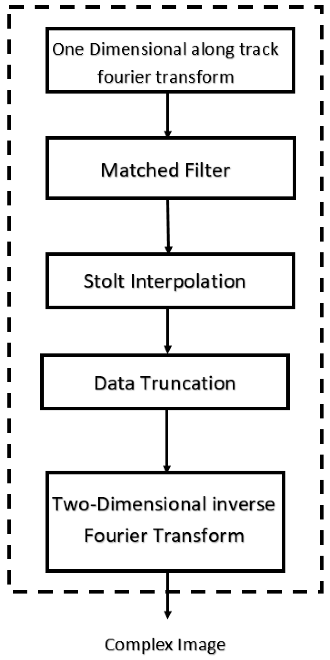
where is the complex reflectivity at the n-th position and m-th frequency and is the two-way propagation delay from the radar to the target. The formulation of the RMA will continue from this input matrix and progress as shown in the block diagram shown in Figure 4.
3.1. Along Track Fourier Transform
The first step of the algorithm is to perform the discrete Fourier transform in the along-track direction. This converts the spatial locations into frequency with units of radians per meter. The frequency in the range direction is scaled by and is denoted by . The frequency after scaling varies between
and
where is the center frequency. The azimuth spatial frequency after the along track FFT is denoted as and varies from to where is the spatial sample spacing. The correction of warping the range extent of a returned signal is done by remapping , which is achieved via Stolt interpolation.
3.2. Matched Filtering
The second step of the algorithm is to perform matched filtering. This operation is to correct the range curvature of the scatterers and match targets to the scene center spatially in the wavenumber domain. It is not the traditional matched filtering in time domain. This operation perfectly corrects the curvature at the scene center range but only partially corrects at other distances. This is done in the azimuth frequency domain rather than the along track position domain. The phase of the matched filter is
At this point, the signal is of the form
After multiplication with the matched filter, it takes the form
The matched filter over compensates for targets further than the scene center and under compensates for targets closer than the scene center. Therefore, we need another operation to complete correcting the curvature of the return signals. This is done using the Stolt interpolation.
3.3. Stolt Interpolation
The Stolt interpolation operation corrects for the range curvature of all of the scatterers in the scene. The spatial frequency of a scatterer varies over . This can be thought of as a sinusoid with increasing frequency. The Stolt interpolation is a one-dimensional mapping from to as a function of . This is like stretching a one dimensional sinusoid to reduce the frequency. The goal is to have a constant frequency over which would in a sense straighten out the signal. The mapping to is done using
After this interpolation, the range curvature has been corrected for all the scatterers. Now the signal needs to be truncated in the wavenumber domain to suppress spatial invariant side lobes. Rewriting in terms of and , in Equation (14) can be expressed as .
3.4. Space-Variant Impulse Response
In spotlight SAR, the azimuth angles over which the aperture observes each scatterer varies. Therefore each scatterer returns a varying amount of range walk that contributes a linear component to the azimuth spectrum that shifts the spectrum center to a non-zero carrier frequency [45]. The size of this carrier frequency varies with the range-walk, so it varies with the scatterer’s position. Thus, the spectra in the wavenumber domain will be slightly shifted with respect to each other depending on their position in the scene. This causes the processing aperture to vary with respect to the different scatterers after the 2D inverse Fourier transform. To correct for this, the wavenumber domain can be truncated after the Stolt interpolation to only include a rectangular processing aperture. This truncation makes it so that the spectra of each scatterer are processed by a common aperture. This corrects the distribution of the side lobes caused by the space-variant impulse response. A Hanning window can also be applied in range and azimuth before or after the data truncation. The Hanning window is described by
The Hanning window suppresses the first sidelobe to −31.5 dB but also widens the −3 dB response of the target. Overall, this is beneficial in this application because precise resolution in range and azimuth is not the goal. The more important application is to determine the precise number of unique targets behind the wall.
3.5. 2D Inverse Fourier Transform
The two-dimensional inverse Fourier transform can now be performed on to compress the range and azimuth scatterers into the imaging domain . The 2D inverse discrete Fourier transform can be easily computed in MATLAB.
3.6. Range Migration Algorithm Results
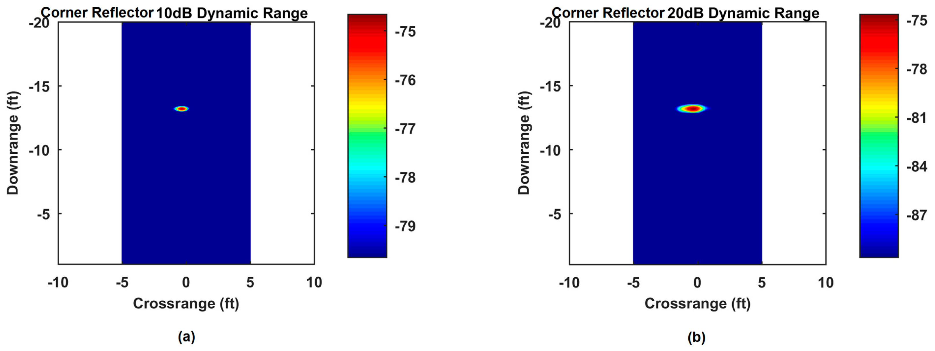
The range migration algorithm was used to image a corner reflector through a wall as a baseline case to compare other images to. The corner reflector was placed 3.96 m (13 feet) centered down-range. The wall material used was concrete. The antenna array was at a standoff distance of 0.3 m (1 foot). A target scene case and an empty range set case were used to background subject stationary clutter such as the wall response. Figure 5 shows the images formed by the RMA from 10 to 50 dB image dynamic range. A D-dB dynamic range means that all pixel values lower than D-dB below the peak value were set to zero. The corner reflector is localized in both down-range and cross-range extents. The sidelobes only start to appear significantly past 30-dB dynamic range.
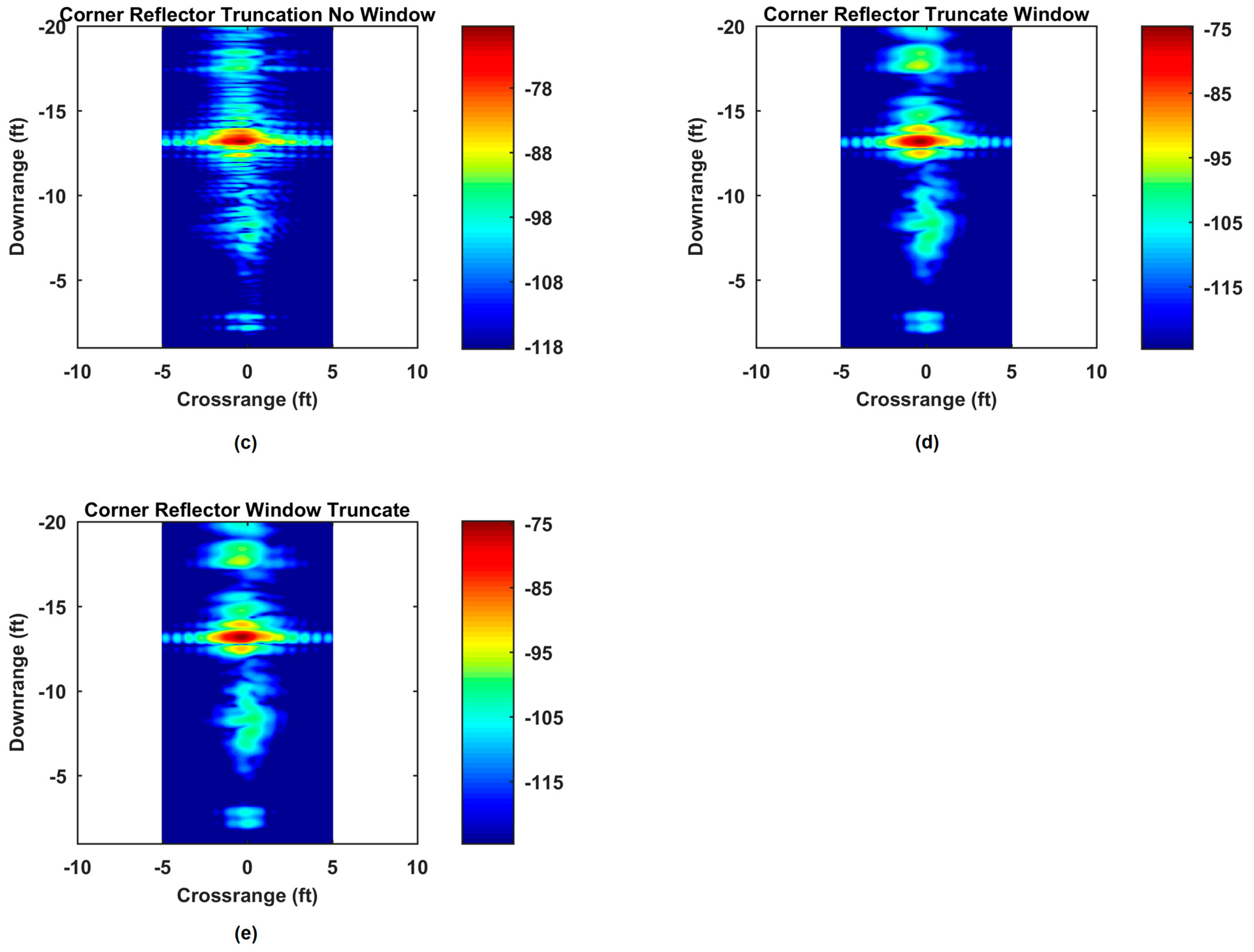
Figure 6 shows the corner reflector imaged at 50-dB dynamic range with varying applications of windows and data truncation. When no data truncation is applied, the corner reflector shows distorted side lobes and is also stretched out the cross-range extent. After data truncation, the return from the corner reflector is more focused in the cross-range extent and the sidelobes are no longer distorted. The application of the Hanning window before and after truncating the data is also examined. The application of the window after the truncation reduces the sidelobes more significantly than after the truncation because the Hanning window is smaller and the weights are larger. However, the 3-dB response from the target is also widened as expected. The application of the window after the truncation gives the best tradeoff between resolution and side lobe reduction.
It can be seen that the RMA can completely compensate motion through range cells. Large scenes do not suffer from geometric distortions using the RMA. More importantly for short range systems, the RMA corrects the range curvature of every scatterer in the scene simultaneously. The RMA is also computationally comparable to other algorithms and has been used for real time through-wall imaging systems up to 10-Hz frame rate [49]. These considerations make the RMA an ideal algorithm for use in short range through-wall radar systems.
3.7. Data Calibration Process
A calibration process exists to calibrate the virtual array to a known scatterer’s scene center for use with the RMA [47]. This calibration is useful in uncalibrated radar systems using this imaging technique [48]. The calibration can be performed for any target that has a large radar cross section and resembles a point target. For example, a corner reflector or metal pole could be used as a calibration target. The calibration target should be placed centered down-range at a range to the calibration target scene center. A background scene should also be measured to eliminate noise from clutter in the scene. The calibration measurement can therefore be represented as
Now, a theoretical return from a point target at the same distance can be formulated as
in which is given by
where is the cross-range position of the target and is the down-range position of the target. Therefore, if the target is centered downrange (), Equation (19) reduces to the distance down-range to the target.
Now, a calibration factor can be obtained by taking the ratio of the quantities from Equations (17) and (18) as
This calibration factor can then be applied to the experimental data.
Now, the array is calibrated based on that geometry. The calibration factor can be preloaded and applied to new input data.
4. Multi-View Through-Wall Imaging Results
A multi-wall (two walls at right angles) view was investigated to try to improve the detection and localization of targets through wall. The motivation for this is to suppress side lobes and multi path returns associated with through wall SAR imagery [50]. These sidelobes and multipath image artifacts can be misinterpreted as true targets and there is a requirement to create images of higher dynamic range to reduce false positives and increase true positives. To accomplish these improvements, a multi-view data fusion approach was investigated by creating two images of the same scene imaged from viewing angles that are at 90 degrees to each other. This allows for rotation of the images to accomplish image fusion using methods that are not computationally expensive and can provide significant improvements as opposed to single view imagery. The tradeoff for this method is greater hardware requirements as well as communication between independent radar units.
This work investigated two scenarios. The scenarios were a single target from two views and two targets from two views. Figure 7 shows the multi-view through-wall radar setup. These were chosen to show how this method can be used to improve some of the challenges with imaging both scenarios. Figure 5 and Figure 6 illustrated the problem of sidelobes and image artifacts as the dynamic range of the image increases. To address this, the two scenarios were examined, and the advantages will be discussed.
4.1. Multi-Wall Processing Approach
For exploring multi-wall fusion, a typical geometry was assumed for the target location(s) from each 90-degree wall, and data collected using this arrangement from the single available wall at the respective distances. One of the datasets was then appropriately rotated to simulate the view from the right-angled wall and the combined data were fused.
The multi-wall fusion is performed by rotating the pixels from the formed image by 90 degrees to overlap with the pixels from another image. The rotation of the pixels can also be arbitrary and can be represented by the follow transformation
where and are the 2D coordinates of the original pixel, and are the transformed pixel coordinates, and is the angle of the wall view with respect to the primary wall view. This transformation is valid for clockwise rotation of angle . In our case, is 90 degrees. The primary wall view can be selected arbitrarily.
After the rotation, the images need to be truncated to an area of common overlap. This is done in the processing of the RMA because the data can be truncated to any arbitrary down-range and cross-range extent. By performing this truncation, the images can then be fused to provide improvements to the data.
First, the two images should be normalized to account for differences in path length and scene to scene multipath and miscellaneous system losses [51]. The normalization of the formed images can be described as
where the maximum pixel value of scene in the denominator and the numerator is the n-th pixel in k-th scene produce the image with normalized values. The scenes can then be fused using multiplicative combining. Multiplicative combining can be represented by the following equation
where is the total number of scenes (two, in our case).
This can improve the image quality because the target remains in the same location in each image, but returns due to multipath, image artifacts, and noise generally vary with each image scene [51].
4.2. Single Target Scene
This scenario had a single target downrange from views of 2.13 m (7 feet) and 3.96 m (13 feet) respectively. The targets were both centered in cross-range. The wall was made of cinder-blocks dry stacked.
4.2.1. Single Target View 1
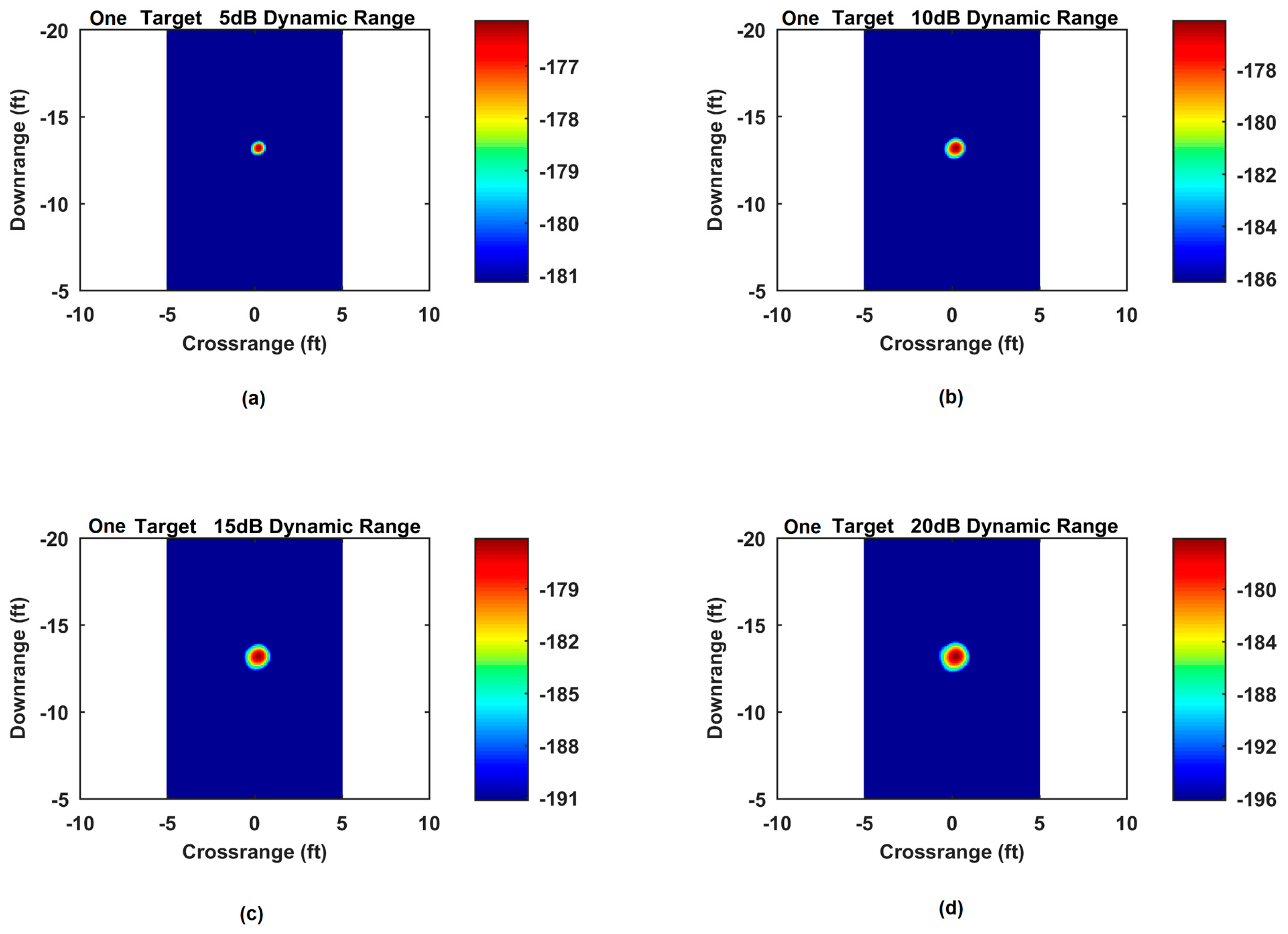
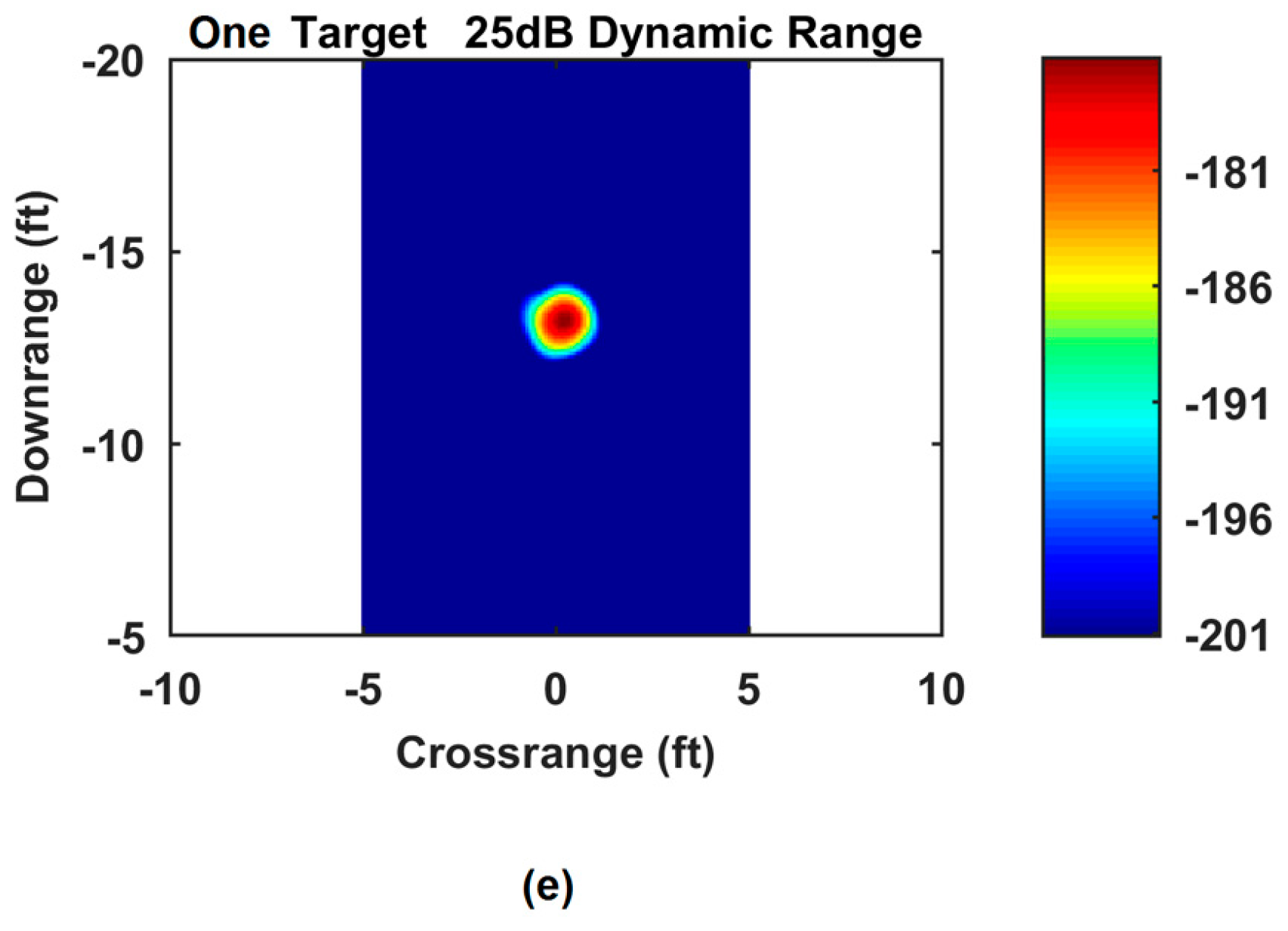
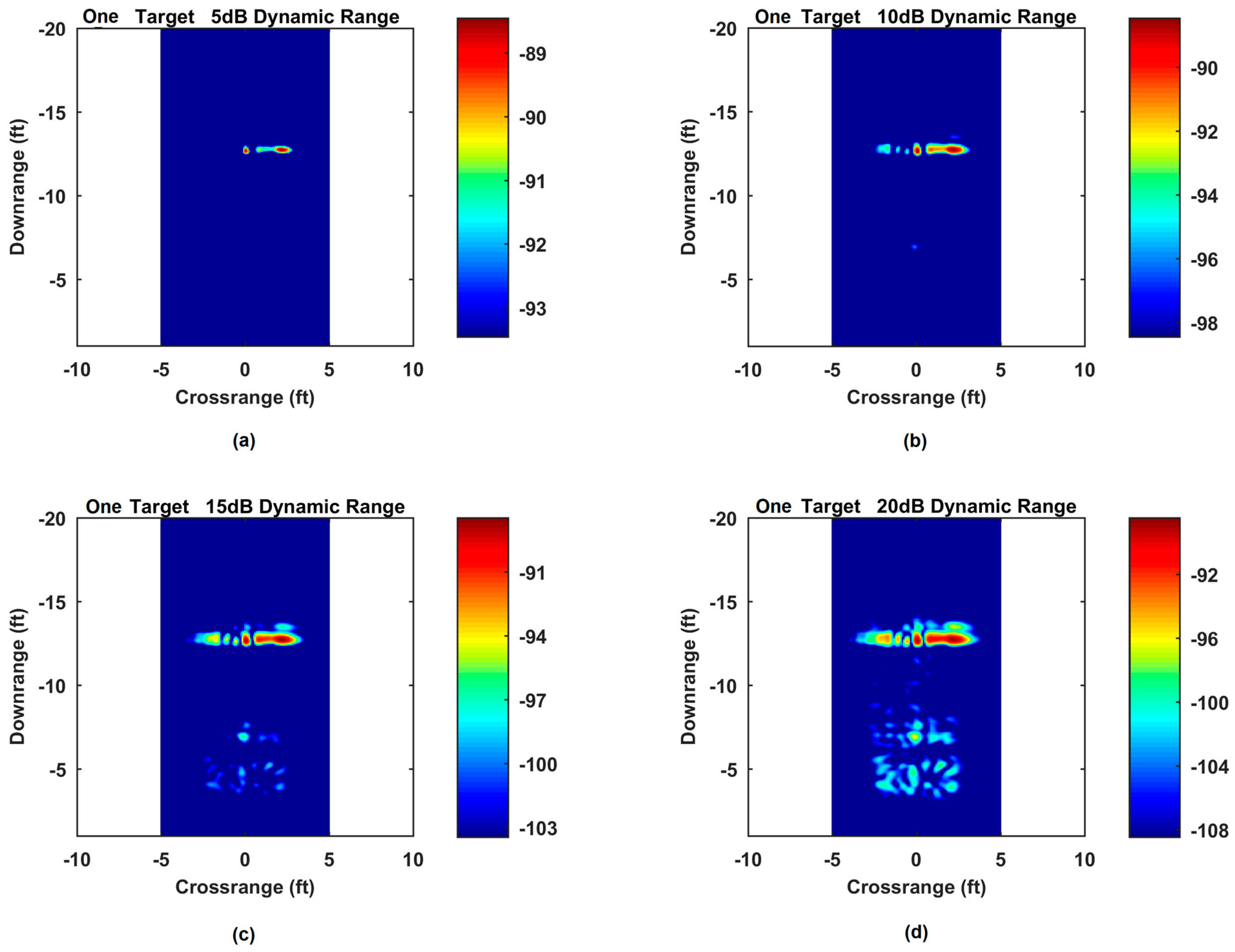
The target was imaged through the wall. Figure 8 shows the images produced by imaging the target 2.13 m (7 feet) down-range through a single wall. The image target can be clearly seen up to 20 dB image dynamic range. Although not shown, beyond a 30 dB image dynamic range, the target starts to spread in cross-range and a second target appears to form next to the main target, as the sidelobes start to appear past 30 dB.
4.2.2. Single Target View 2
This case shows the target image at a distance of 3.96 m (13 feet) down-range, where it can clearly be seen in Figure 9. As before, beyond 30 dB image dynamic range, it was noted that the sidelobes appeared stronger and could begin to be misinterpreted as a second target.
4.3. Multiple Target Scene
This scenario had two targets imaged from two different wall views. In the first view, the targets were about 4.27 m (14 feet) and 3.2 m (10.5 feet) down-range separated by about 1.52 m (5 feet). In the second view, the targets were at about 4.57 m (15 feet) and 3.35 m (11 feet) down-range and separated by the same distance.
4.3.1. Multiple Target View 1
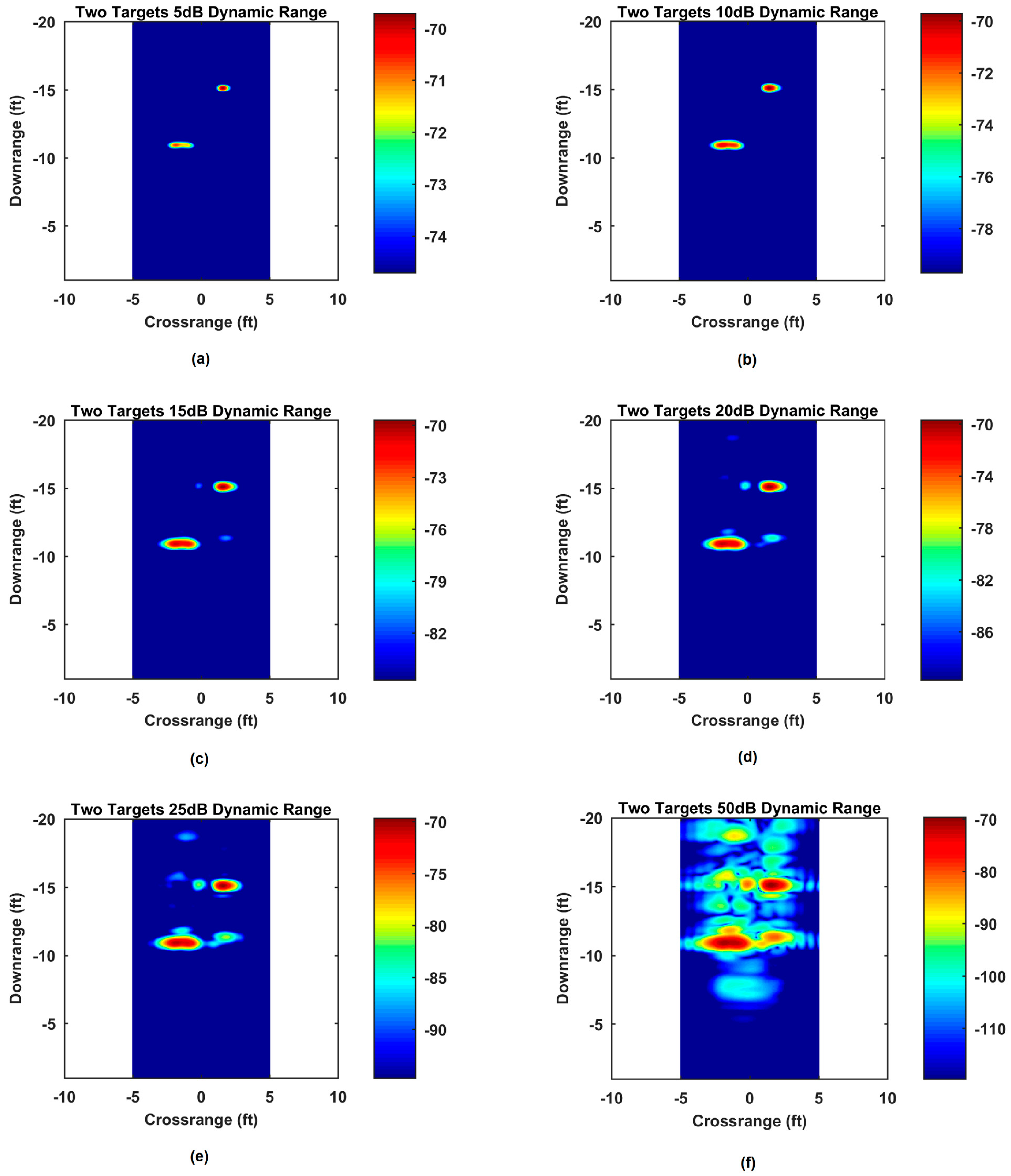
The two targets from View 1 can be seen in Figure 10. The two targets are clearly visible at 20 dB image dynamic range, but beyond that, the sidelobes from the stronger target start to rival the weaker target response in magnitude.
4.3.2. Multiple Target View 2
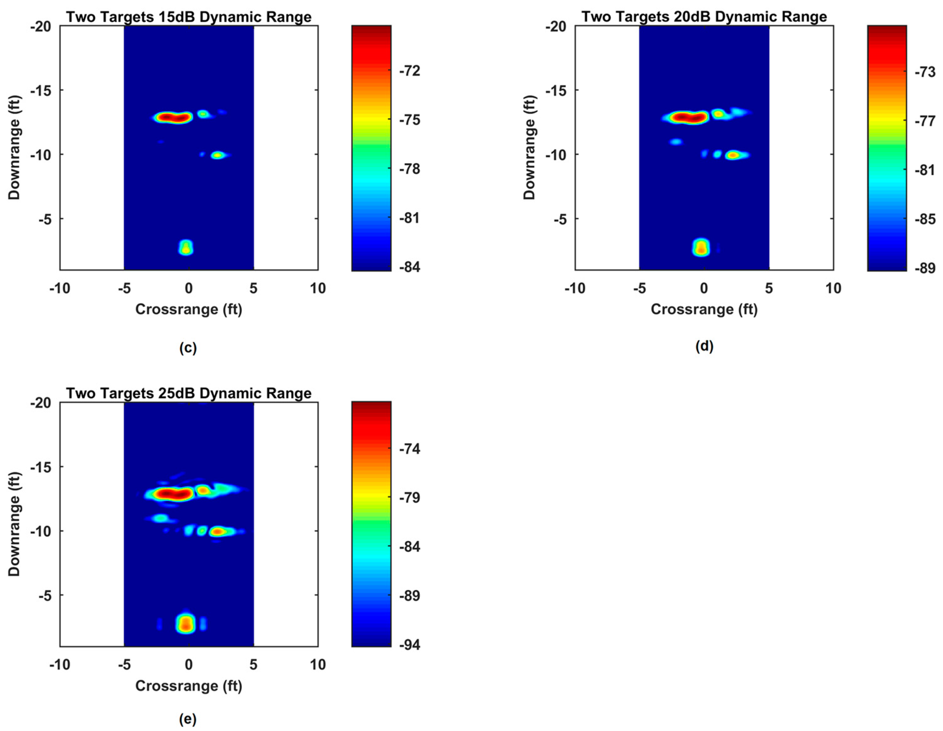
The two targets from View 2 can be seen in Figure 11. The two targets in this scenario can be distinguished up to 30-dB image dynamic range before sidelobes start presenting an issue. In this view, the two targets contribute more equal magnitude responses.
4.4. Two Wall Image Fusion
The images of the two views were fused using Equation (24). The results from these fusions are shown in the following sections.
4.4.1. Single Target
The fusion of the single target view can be seen in Figure 12 and Figure 13. The image is fused from the perspective of the target from 3.96 m (13 feet) down-range. The fusion of the target views from the two perspectives shown in Figure 8 and Figure 9 shows a clear target response up to even a 50-dB image dynamic range with minimal sidelobe response. However, the target is slightly spread in the down-range and cross-range extent; overall, however, the image can be seen to a dynamic range of 20 dB higher than from each single wall view.
4.4.2. Multiple Targets
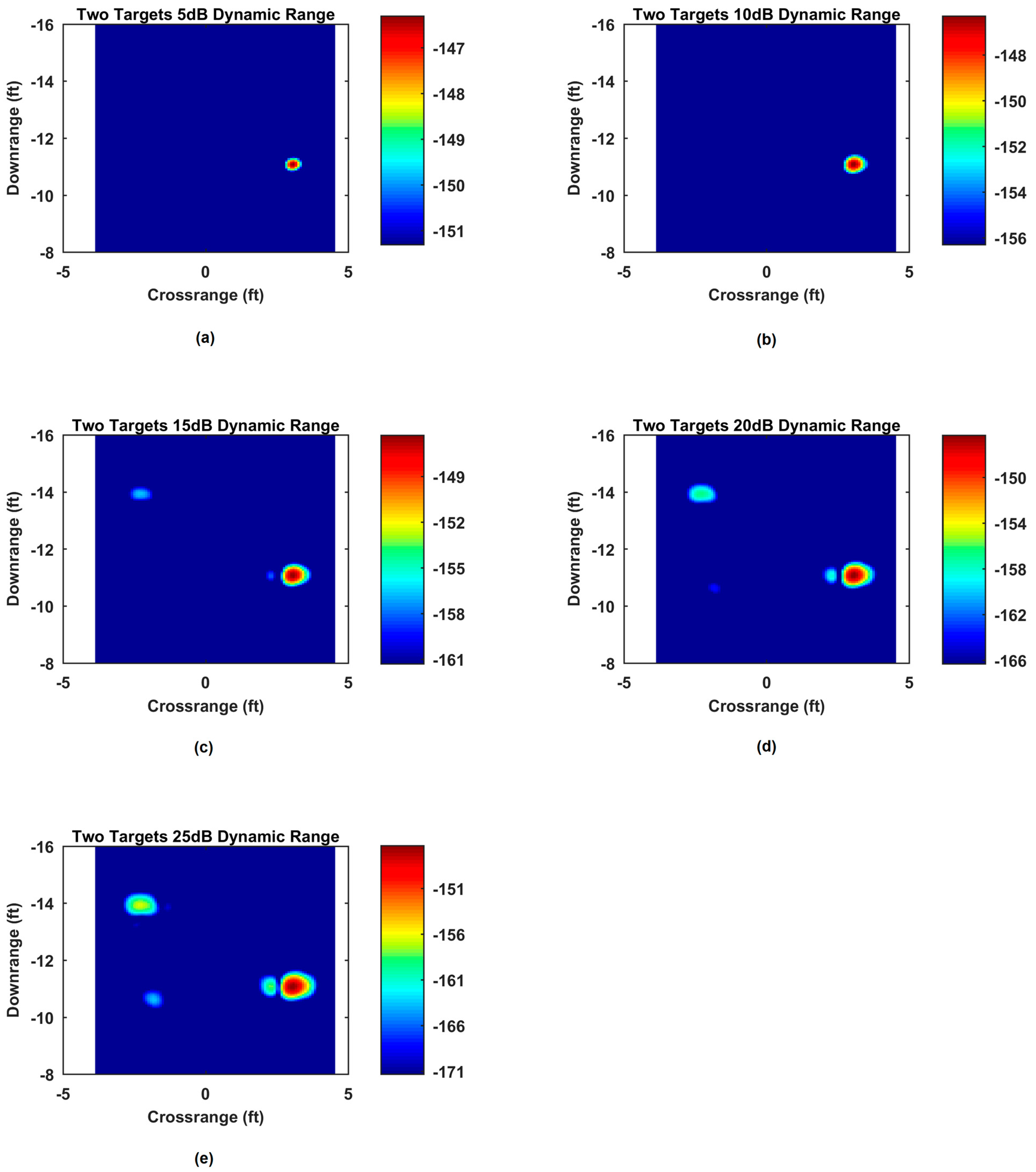
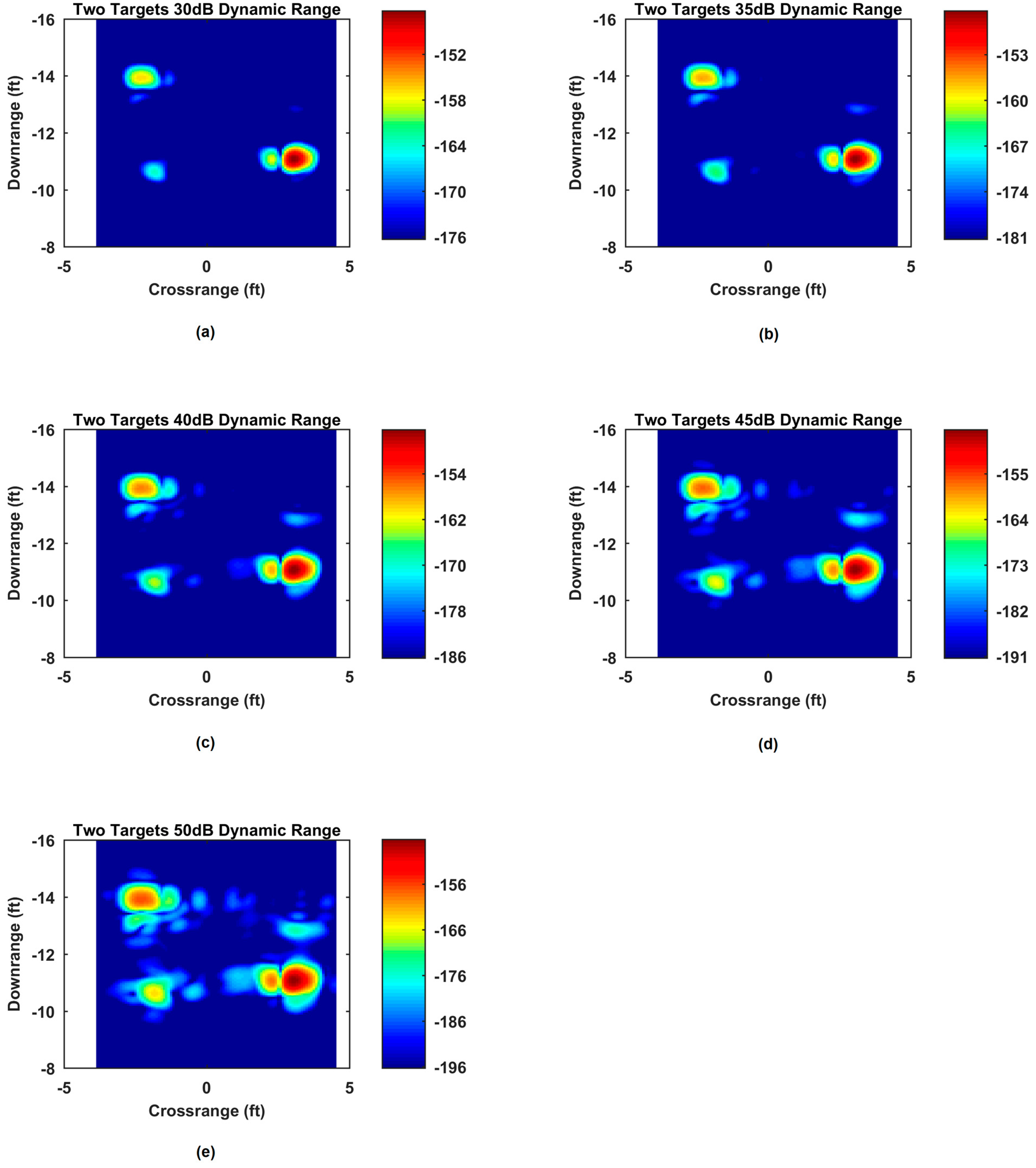
The fusion of the multiple target view can be seen in Figure 14 and Figure 15. The image was fused from the perspective of View 1 of the multiple target scene. The fusion of the two targets suppresses the side lobes and the two targets can be imaged up to 50 dB image dynamic range. However, the weaker target response only shows up after about 20 dB dynamic range. Therefore, while the two distinct targets can still be clearly imaged, the target responses on different scales still pose difficulties to successfully detect both targets.
5. Wavelet-Singular Value Decomposition (Wavelet-SVD) Approach
The images obtained using the RMA approach show relatively high sidelobes beyond 20 dB image dynamic range. The two-wall fusion technique succeeded in suppressing sidelobes, but at the cost of greater hardware requirements. In addition, the technique requires the use of some form of background subtraction to remove the response from the wall and other stationary clutter. A method that produces images with low sidelobes and no background subtraction is desirable, which will relax hardware and processing requirements.
To achieve the desired results without using background subtraction, an approach using the wavelet transform was utilized. The wavelet transform gives the notion of resolution and scale. The inspiration for this method comes from wavelet denoising. In wavelet denoising, a multi-level wavelet transform is used to threshold out the noise from an image at different scales. In wavelet denoising, the noise is much weaker than the actual image. However, in through-wall radar, the wall response is much stronger than the target response. So instead of thresholding out the coefficients that represent the noise, the coefficients that contain the wall response can be thresholded to remove it. The wavelet coefficients can be operated on by a singular value decomposition (SVD). Large singular values represent the wall response and can be removed. The SVD outcome can be reversed, and the inverse wavelet transform can be used to return to the radar return domain.
A new image can then be formed using the RMA from Section 3. In this section, we provide a brief review and then examine both the SVD approach to mitigate the wall response, and the wavelet-SVD method to remove the wall response. The use of a SVD for filtering singular values has been explored and its merits convincingly established [52,53].
5.1. Singular Value Decomposition (SVD)
A matrix , in the form of Equation (9), can be decomposed using SVD, which is described as
where is a matrix whose columns are the orthonormal eigenvectors of , is a matrix whose columns are the orthonormal eigenvectors of , and the diagonal matrix represents the singular values of the matrix in terms of the square roots of the eigenvalues. These values are ordered from greatest to least magnitude and represent the diagonal matrix where is the largest singular value and is the smallest singular value.
The first singular value represents the best rank 1 approximation of the matrix [54]. For the matrix , each successive singular value represents the next best rank 1 approximation of the matrix. For the application to through-the-wall radar, the largest singular values will represent the returns from the wall. After some value , where , the singular values will start to represent the target space. So, by the removal of these singular values, the response from the wall can be removed from a data matrix . This fact will be used for the SVD wall mitigation method as well as the wavelet-SVD method. To reverse the SVD, the terms can be recollected after the desired singular values are nulled and the data matrix can be recovered using Equation (25).
5.2. 2-D Wavelet Transform
A 2D Wavelet Transform can be performed on the input matrix S. This can be represented as a series of 1D filters and downsample operations as shown in Figure 16 [55,56]. The resulting cascade of filters gives four sub-bands {A, H, V, D}. Each of these sub-bands can be the new input matrix S in Equation (26). The number of singular values to remove from each sub-band, , was chosen based on experience after working with several images.
For this application, a wavelet basis is selected based on how much it resembles the signal trying to be recovered. For our application, the Daubechies 8 and bior 6.8 bases gave the best results. The filters in Figure 16 can be cascaded to decompose the 2D matrix into different decomposition levels. Each of these levels contributes a new set of sub-bands, and each sub-band can be operated on. An inverse discrete wavelet transform can be taken to recover the matrix back into the original input signal domain. This signal can then be used to image the scene. The matrix containing the radar returns can be decomposed by Equation (25) to the form
This denotes the SVD of the input signal matrix. The wall subspace can be defined as
where is the index of the singular value which includes the singular values of the wall. The orthogonal subspace to the wall is
Hence, the wall response can be removed by the following equation
The new matrix shown in Equation (29) has now mitigated the wall response by effectively zeroing out the singular values associated with the wall response [53]. This can either be done once in the case of the simple SVD wall mitigation, or done for each sub-band as is the case for the wavelet-SVD method.
5.3. Wall Effect Mitigation Using SVD
For these images, the wall clutter was mitigated without background subtraction using the SVD decomposition. This removed the singular values associated with the wall response to enhance the target.
5.3.1. Single Target
In the single target case located at 3.96 m (13 feet) down-range, the wall response was successfully removed. However, at higher image dynamic ranges, the sidelobes start to become indistinguishable from the main target response. Figure 17 shows the responses. Anything over 10-dB image dynamic range can be regarded as multiple targets and it becomes difficult to distinguish the target from sidelobe responses.
5.3.2. Multiple Targets
The multiple target case has similar performance, as shown in Figure 18. Targets are placed at 3.35 (11 feet) and 4.57 m (15 feet) down-range. The wall response has been successfully mitigated but the two targets are hard to be independently resolved beyond the 10 dB image dynamic range. The two targets are difficult to image together because of their different amplitude responses.
5.4. Wall Effect Mitigation Using Wavelet-SVD
These images were created using the wavelet-SVD based wall mitigation technique. The images were created with a Daubechies 8 filter and using a three-level decomposition. Similar to the SVD case, wall clutter was mitigated without background subtraction.
5.4.1. Single Target
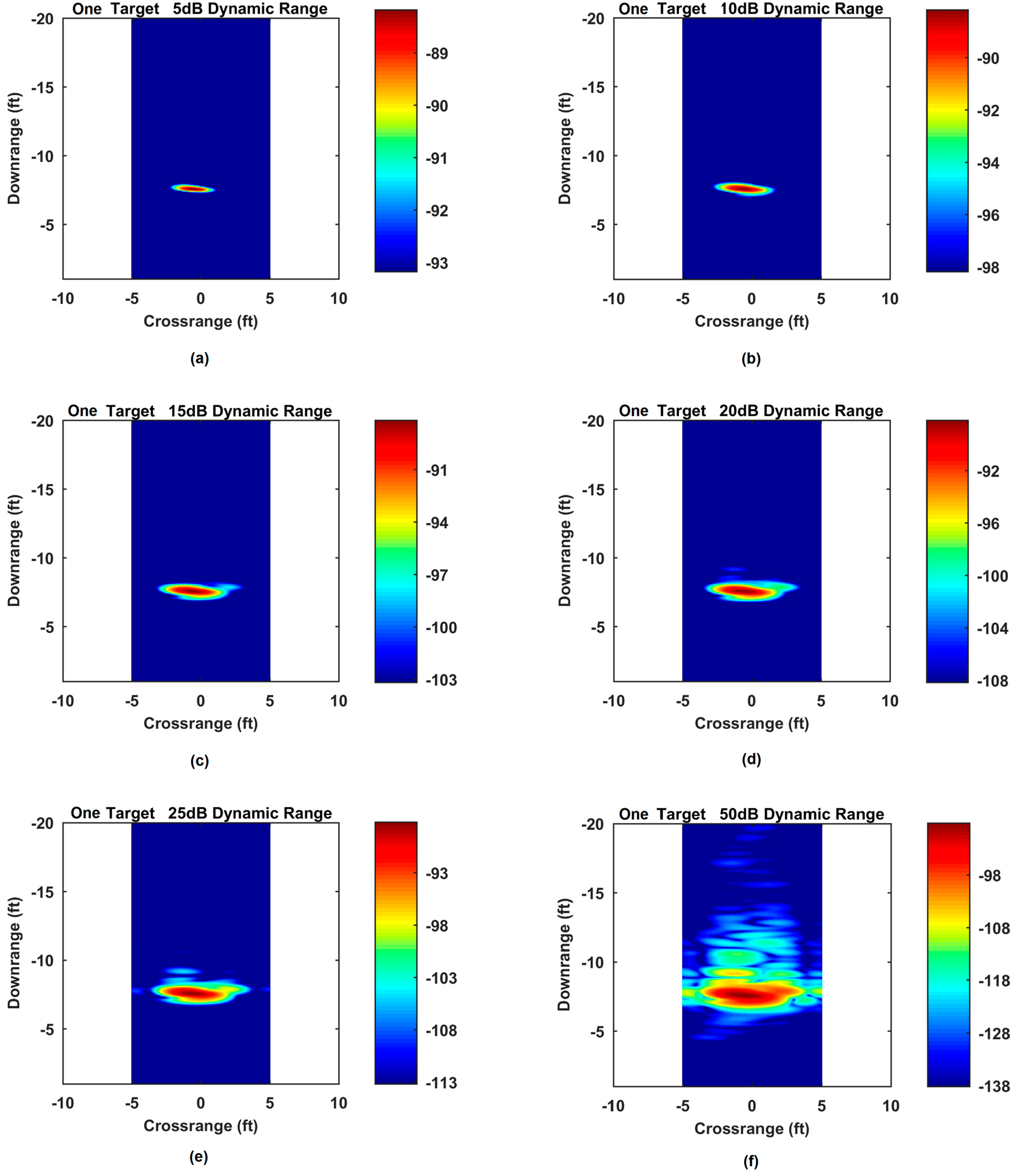
The single target images from the target at 2.13 m (7 feet) down-range show that in this case the performance is good all the way up to 50-dB image dynamic range. The target shows some spreading in cross-range but it still suppresses the side lobes well. Figure 19 shows this case.
5.4.2. Multiple Targets
The multiple target case with targets placed at 3.35 (11 feet) and 4.57 m (15 feet) down-range shows that the wavelet-SVD method performs quite well with multiple targets. Figure 20 shows the response. Both of the targets imaged are clearly visible up to 50 dB image dynamic range with no significant sidelobes or image artifacts.
6. Image Analysis
We propose and use the target-to-clutter ratio (TCR) as a metric to perform quantitative comparisons between the various approaches. This metric has been used in other through the wall radar work [52]. We define TCR as
where and are the target and clutter regions of the image , respectively, and and are the number of image pixels in the target and clutter regions, respectively. Any pixel that does not belong to the known target region is considered a clutter pixel.
From Table 1, we infer that combined truncation and windowing improves the TCR by about 6.6 dB compared to the no truncation and no windowing case. When one of these operations is performed, the TCR improves by about 5.3 dB.
Table 2 reveals that image fusion significantly enhances the TCR by about 21 dB for the single target case compared to just using background-subtracted data from a single wall. However, from Table 3, we note that similar improvement is not as dramatic for the multiple target case, but still significant at about 7 dB.
Finally, Table 4 shows that the wavelet approach outperforms the SVD approach, with TCR improvements ranging from 18.2 dB for the single target and 15.8 dB for the multiple target cases, respectively.
7. Conclusions
This paper presented and discusses several approaches for MIMO radar imaging of single and multiple targets through walls and presented extensive experimental results on different techniques investigated. The virtual array configuration was employed to collect data with a lower number of elements compared to a conventional linear array. For the RMA approach, multi-look images from orthogonal aspect views were fused to localize and image single and multiple targets with excellent down-range and cross-range resolutions after implementing image subtraction to reduce wall clutter. A data truncation operation was applied to improve upon existing implementations of the algorithm. To overcome the need for image subtraction which may not always be an option, the SVD and the wavelet-SVD approaches were investigated to directly excise the strong response due to the wall and perform further processing to obtain high-range resolution localization of single and multiple targets.
The methods presented can be applied to any uniform linear array configuration of through-the-wall radar data. The imagery can be used as the final images of a through wall system, or be another input to further processing such as constant false alarm rate (CFAR) detection or tracking. Future work in this area could address the choice of wavelet bases for the wavelet method, as well as choice of appropriate wavelet coefficients to mitigate at each decomposition level.
Acknowledgments
This research was supported by U.S. Army CERDEC through The Pennsylvania State Applied Research Laboratory Contract # N00024-12-D-6404 (Delivery Order 0326).
Author Contributions
All authors equally conceived and designed the experiments; R.M.N. proposed and developed the concept; E.T.G. performed the experiments; all authors analyzed the data; S.P.B. contributed the logistics and hardware; R.M.N. wrote the first draft of the paper, and other authors contributed to its final form.
Conflicts of Interest
The authors declare no conflict of interest. The funding sponsors had no role in the design of the study; in the collection, analyses, or interpretation of data; in the writing of the manuscript, and in the decision to publish the results.
References
- Anonymous. Radar senses through wall. Eng. Mater. Des. 1976, 20, 34. [Google Scholar]
- Azevedo, S.; McEwan, T.E. Micropower impulse radar. IEEE Potentials 1997, 16, 15–20. [Google Scholar] [CrossRef]
- Nag, S.; Fluhler, H.; Barnes, M. Preliminary interferometric images of moving targets obtained using a time-modulated ultra-wide band through-wall penetration radar. In Proceedings of the 2001 IEEE Radar Conference, Atlanta, GA, USA, 1–3 May 2001; pp. 64–69. [Google Scholar]
- Yang, Y.; Fathy, A.E. See-through-wall imaging using ultra wideband short-pulse radar system. In Proceedings of the 2005 Antennas and Propagation Society International Symposium, Washington, DC, USA, 3–8 July 2005. [Google Scholar] [CrossRef]
- Falconer, D.G.; Steadman, K.N.; Watters, D.G. Through-the-wall differential radar. In Proceedings of the SPIE Conference on Command, Control, Communications, and Intelligence Systems for Law Enforcement, Boston, MA, USA, 18–22 November 1996; pp. 147–151. [Google Scholar]
- Maaref, N.; Millot, P.; Pichot, C.; Picon, O. A study of UWB FM-CW radar for the detection of human beings in motion inside a building. IEEE Trans. Geosci. Remote Sens. 2009, 47, 1297–1300. [Google Scholar] [CrossRef]
- Ahmad, F.; Amin, M.G.; Zemany, P.D. Dual-frequency radars for target localization in urban sensing. IEEE Trans. Aerosp. Electron. Syst. 2009, 45, 1598–1609. [Google Scholar] [CrossRef]
- Zetik, R.; Crabbe, S.; Krajnak, J.; Peyerl, P.; Sachs, J.; Thomä, R. Detection and localization of persons behind obstacles using M-sequence through-the-wall radar. In Proceedings of the SPIE Conference on Sensors, and Command, Control, Communications, and Intelligence (C3I) Technologies for Homeland Security and Homeland Defense V, Orlando, FL, USA, 17–21 April 2006; pp. 62010I-1–62010I-12. [Google Scholar]
- Rišková, M.; Rovňáková, J.; Aftanas, M. M-sequence UWB radar architecture for through-wall detection and localisation. In Proceedings of the 7th PhD Student Conference and Scientific and Technical Competition of Students of Faculty of Electrical Engineering and Informatics, Košice, Slovakia, 25 May 2007; pp. 29–30. [Google Scholar]
- Lukin, K.; Konovalov, V. Through wall detection and recognition of human beings using noise radar sensors. In Proceedings of the NATO RTO SET Symposium on Target Identification and Recognition Using RF Systems, Oslo, Norway, 11–13 October 2004; pp. P15-1–P15-12. [Google Scholar]
- Lai, C.P.; Narayanan, R.M. Ultrawideband random noise radar design for through-wall surveillance. IEEE Trans. Aerosp. Electron. Syst. 2010, 46, 1716–1730. [Google Scholar] [CrossRef]
- Chen, P.H.; Shastry, M.C.; Lai, C.P.; Narayanan, R.M. A portable real-time digital noise radar system for through-the-wall imaging. IEEE Trans. Geosci. Remote Sens. 2012, 50, 4123–4134. [Google Scholar] [CrossRef]
- Sachs, J.; Aftanas, M.; Crabbe, S.; Drutarovský, M.; Klukas, R.; Kocur, D.; Nguyen, T.T.; Peyerl, P.; Rovňáková, J.; Zaikov, E. Detection and tracking of moving or trapped people hidden by obstacles using ultra-wideband pseudo-noise radar. In Proceedings of the 2008 European Radar Conference, Amsterdam, The Netherlands, 27–31 October 2008; pp. 408–411. [Google Scholar]
- Venkatasubramanian, V.; Leung, H. Chaos UWB radar for through-the-wall imaging. IEEE Trans. Image Process. 2009, 18, 1255–1265. [Google Scholar] [CrossRef] [PubMed]
- Xu, H.; Wang, B.; Zhang, J.; Liu, L.; Li, Y.; Wang, Y.; Wang, A. Chaos through-wall imaging radar. Sens. Imaging 2017, 18. [Google Scholar] [CrossRef]
- Slimane, Z.; Abdelmalek, A.; Feham, M. OFDM based UWB synthetic aperture through-wall imaging radar. In Proceedings of the 3rd International Conference on Broadband Communications, Information Technology & Biomedical Applications, Pretoria, South Africa, 23–26 November 2008; pp. 293–300. [Google Scholar]
- Jameson, B.; Curtis, A.; Garmatyuk, D.; Morton, Y.T.J.; Plummer, P.; Thompson, K. Detection of behind-the-wall targets with adaptive UWB OFDM radar: Experimental approach. In Proceedings of the 2011 IEEE Radar Conference, Kansas City, MO, USA, 23–27 May 2011; pp. 945–950. [Google Scholar]
- Frazier, L.M. Radar surveillance through solid materials. In Proceedings of the SPIE Conference on Command, Control, Communications, and Intelligence Systems for Law Enforcement, Boston, MA, USA, 18–22 November 1996; pp. 139–146. [Google Scholar]
- Muqaibel, A.; Safaai-Jazi, A.; Bayram, A.; Attiya, A.M.; Riad, S.M. Ultrawideband through-the-wall propagation. IEE Proc. Microw. Antennas Propag. 2005, 152, 581–588. [Google Scholar] [CrossRef]
- Muqaibel, A.; Safaai-Jazi, A. Characterization of wall dispersive and attenuative effects on UWB radar signals. J. Frankl. Inst. 2008, 345, 640–658. [Google Scholar] [CrossRef]
- Greneker, G.; Rausch, E.O. Wall characterization for through-the-wall radar applications. In Proceedings of the SPIE Conference on Radar Sensor Technology XII, Orlando, FL, USA, 18–19 March 2008. [Google Scholar] [CrossRef]
- Fishler, E.; Haimovich, A.; Blum, R.; Chizhik, D.; Cimini, L.; Valenzeuela, R. MIMO radar: An idea whose time has come. In Proceedings of the 2004 IEEE Radar Conference, Philadelphia, PA, USA, 26–29 April 2004; pp. 71–78. [Google Scholar]
- Forsythe, K.W.; Bliss, D.W. MIMO radar: Concepts, performance enhancements, and applications. In MIMO Radar Signal Processing; Li, J., Stoica, P., Eds.; Wiley: Hoboken, NJ, USA, 2009; pp. 65–121. [Google Scholar]
- Brookner, E. MIMO radar: Demystified. Microw. J. 2013, 56, 22–44. [Google Scholar]
- Van Rossum, W.L.; Huizing, A.G. Comparison of MIMO radar concepts: Detection performance. In Proceedings of the 2007 IET International Conference on Radar Systems, Edinburgh, UK, 15–18 October 2007. [Google Scholar] [CrossRef]
- Li, J.; Stoica, P. MIMO radar with colocated antennas: Review of some recent work. IEEE Signal Process. Mag. 2007, 24, 106–114. [Google Scholar] [CrossRef]
- Haimovich, A.M.; Blum, R.S.; Cimini, L.J., Jr. MIMO radar with widely separated antennas: Reviewing recent work. IEEE Signal Process. Mag. 2008, 25, 116–129. [Google Scholar] [CrossRef]
- Hassanien, A.; Vorobyov, S. Phased-MIMO radar: A tradeoff between phased-array and MIMO radars. IEEE Trans. Signal Process. 2010, 58, 3137–3151. [Google Scholar] [CrossRef]
- Lamanna, M.; Fuhrmann, D. Cramer-Rao lower bounds comparison for 2D Hybrid–MIMO and MIMO radar. IEEE J. Sel. Top. Signal Process. 2017, 11, 404–413. [Google Scholar] [CrossRef]
- Lehmann, N.H.; Haimovich, A.M.; Blum, R.S.; Cimini, L. High resolution capabilities of MIMO radar. In Proceedings of the 40th Asilomar Conference on Signals, Systems and Computers, Pacific Grove, CA, USA, 29 October–1 November 2006; pp. 25–30. [Google Scholar]
- Xu, L.; Li, J.; Stoica, P. Radar imaging via adaptive MIMO techniques. In Proceedings of the 14th European Signal Processing Conference (EUSIPCO), Florence, Italy, 4–8 September 2006. [Google Scholar]
- Zeng, J.K.; Dong, Z.M. The data fusion for MIMO radar. Adv. Mater. Res. 2010, 121–122, 627–632. [Google Scholar] [CrossRef]
- Yarovoy, A.; Cetinkaya, H.; Wang, J. Sparse MIMO array for short-range imaging. In Proceedings of the 9th European Conference on Antennas and Propagation (EuCAP), Lisbon, Portugal, 13–17 April 2015. [Google Scholar]
- Chen, W.J.; Narayanan, R.M. Comparison of the estimation performance of coherent and non-coherent ambiguity functions for an ultrawideband multi-input–multi-output noise radar. IET Radar Sonar Navig. 2012, 6, 49–59. [Google Scholar] [CrossRef]
- Chen, W.J.; Narayanan, R.M. CGLRT plus TDL beamforming for ultrawideband MIMO noise radar. IEEE Trans. Aerosp. Electron. Syst. 2012, 48, 1858–1869. [Google Scholar] [CrossRef]
- Khan, H.A.; Malik, W.Q.; Edwards, D.J.; Stevens, C.J. Ultra wideband multiple-input multiple-output radar. In Proceedings of the 2005 IEEE International Radar Conference, Arlington, VA, USA, 9–12 May 2005. [Google Scholar] [CrossRef]
- Caban, S.; Mehlführer, C.; Langwieser, R.; Scholtz, A.L.; Rupp, M. Vienna MIMO testbed. EURASIP J. Appl. Signal Process. 2006, 2006, 54868. [Google Scholar] [CrossRef]
- Kpré, E.L.; Fromenteze, T.; Decroze, C.; Carsenat, D. Experimental implementation of an ultra-wide band MIMO radar. In Proceedings of the 12th European Radar Conference (EURAD), Paris, France, 9–11 September 2015; pp. 89–92. [Google Scholar]
- Zhen, Y.; Wei, L.; Qinggong, C.; Dahai, H. Design of a near-field radar imaging system based on MIMO array. In Proceedings of the 12th IEEE International Conference on Electronic Measurement & Instruments (ICEMI), Qingdao, China, 16–18 July 2015; pp. 1265–1269. [Google Scholar]
- Walterscheid, I.; Smith, G.E.; Ender, J.; Baker, C.J. Experimental demonstration of distributed MIMO imaging. In Proceedings of the 11th European Conference on Synthetic Aperture Radar (EUSAR), Hamburg, Germany, 6–9 June 2016. [Google Scholar]
- Zhang, W. Three-dimensional through-the-wall imaging with multiple-input multiple-output (MIMO) radar. J. Electromagn. Waves Appl. 2014, 28, 1935–1943. [Google Scholar] [CrossRef]
- Zankl, D.; Schuster, S.; Feger, R.; Stelzer, A. What a blast! A massive MIMO radar system for monitoring the surface in steel industry blast furnaces. IEEE Microw. Mag. 2017, 18, 52–69. [Google Scholar] [CrossRef]
- McCorkle, J.W. Focusing of synthetic aperture ultra wideband data. In Proceedings of the IEEE International Conference on Systems Engineering, Dayton, OH, USA, 1–3 August 1991; pp. 1–5. [Google Scholar]
- Forsythe, K.W.; Bliss, D.W.; Fawcett, G.S. Multiple-input multiple-output (MIMO) radar: Performance issues. In Proceedings of the Thirty-Eighth Asilomar Conference on Signals, Systems and Computers, Pacific Grove, CA, USA, 7–10 November 2004; pp. 310–315. [Google Scholar]
- Kirschner, A.; Bertl, S.; Guetlein, J.; Detlefsen, J. Comparison and tests of different virtual arrays for MIMO radar applications. In Proceedings of the 12th International Radar Symposium, Leipzig, Germany, 7–9 September 2011; pp. 697–702. [Google Scholar]
- Keep, D.N. Frequency-modulation radar for use in the mercantile marine. Proc. IEEE Part B Radio Electron. Eng. 1956, 103, 519–523. [Google Scholar] [CrossRef]
- Charvat, G.L. Small and Short-Range Radar Systems; CRC Press: Boca Raton, FL, USA, 2014. [Google Scholar]
- Carrara, W.G.; Goodman, R.S.; Majewski, R.M. Spotlight Synthetic Aperture Radar: Signal Processing Algorithms; Artech House: Boston, MA, USA, 1995. [Google Scholar]
- Ralston, T.S.; Charvat, G.L.; Peabody, J.E. Real-time through-wall imaging using an ultrawideband multiple-input multiple-output (MIMO) phased array radar system. In Proceedings of the 2010 IEEE International Symposium on Phased Array Systems and Technology (ARRAY), Waltham, MA, USA, 12–15 October 2010; pp. 551–558. [Google Scholar]
- Papson, S.; Narayanan, R.M. Multiple location SAR/ISAR image fusion for enhanced characterization of targets. In Proceedings of the SPIE Conference on Radar Sensor Technology IX, Orlando, FL, USA, 28 March–1 April 2005; pp. 128–139. [Google Scholar]
- Ahmad, F.; Amin, M.G. Multi-location wideband synthetic aperture imaging for urban sensing applications. J. Frankl. Inst. 2008, 345, 618–639. [Google Scholar] [CrossRef]
- Tivive, F.H.C.; Amin, M.G.; Bouzerdoum, A. Wall clutter mitigation based on eigen-analysis in through-the-wall radar imaging. In Proceedings of the 17th International Conference on Digital Signal Processing (DSP), Corfu, Greece, 6–8 July 2011. [Google Scholar] [CrossRef]
- Tivive, F.H.C.; Bouzerdoum, A. An improved SVD-based wall clutter mitigation method for through-the-wall radar imaging. In Proceedings of the 14th IEEE Workshop on Signal Processing Advances in Wireless Communications (SPAWC), Darmstadt, Germany, 16–19 June 2013; pp. 430–434. [Google Scholar]
- Strang, G. Introduction to Linear Algebra; Wellesley-Cambridge Press: Wellesley, MA, USA, 2009. [Google Scholar]
- Strang, G.; Nguyen, T. Wavelets and Filter Banks; Wellesley-Cambridge Press: Wellesley, MA, USA, 1997. [Google Scholar]
- Mallat, S.G. A theory for multiresolution signal decomposition: The wavelet representation. IEEE Trans. Pattern Anal. Mach. Intell. 1989, 11, 674–693. [Google Scholar] [CrossRef]
- Liu, C.-L. A Tutorial of the Wavelet Transform. Available online: http://disp.ee.ntu.edu.tw/tutorial/WaveletTutorial.pdf (accessed on 10 September 2017).
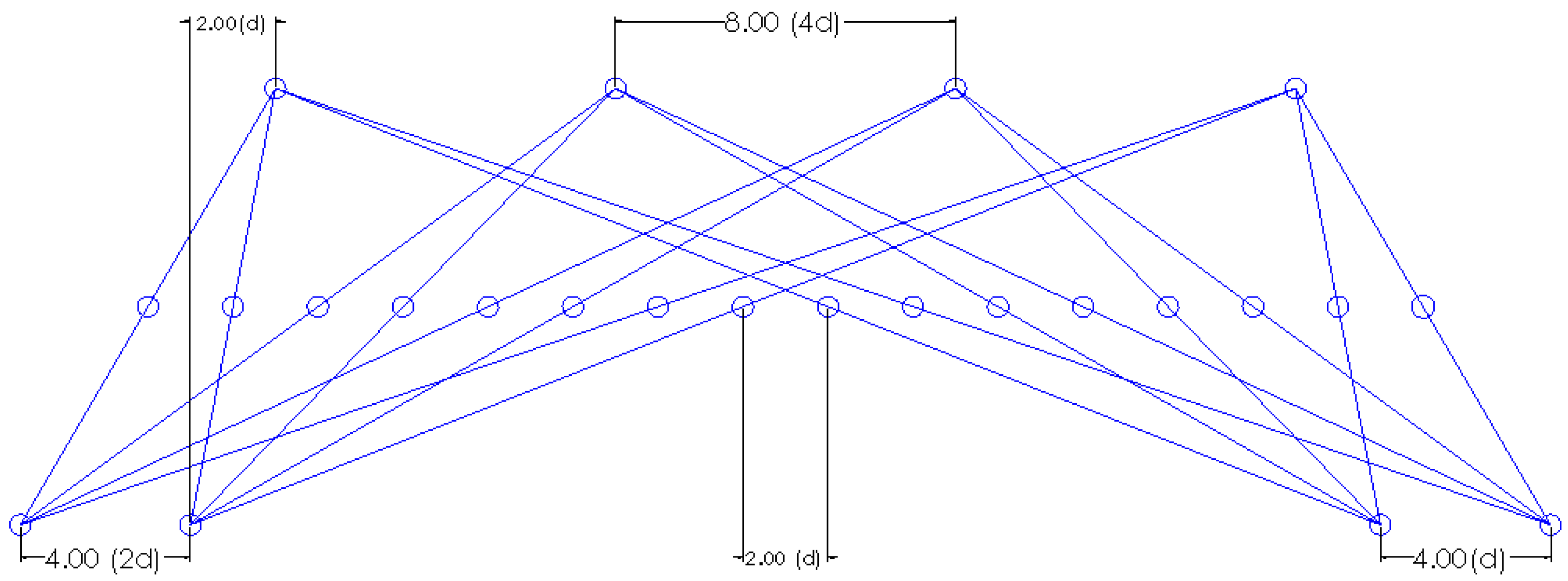
Figure 1.
Virtual antenna array geometry, wherein the top row indicates transmit and the bottom row receive. The middle row is the evenly spaced linear virtual array creating a 4 × 4 array.
Figure 1.
Virtual antenna array geometry, wherein the top row indicates transmit and the bottom row receive. The middle row is the evenly spaced linear virtual array creating a 4 × 4 array.

Figure 2.
Experimental layout for collecting target returns.
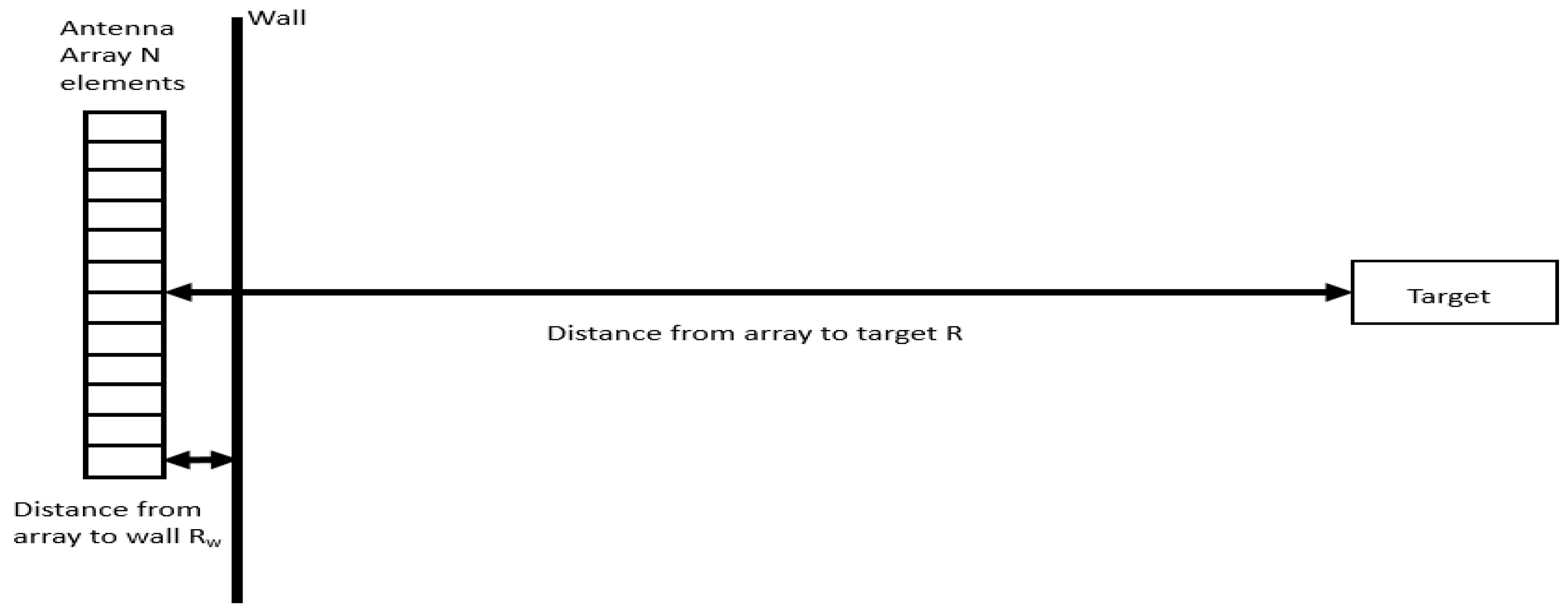
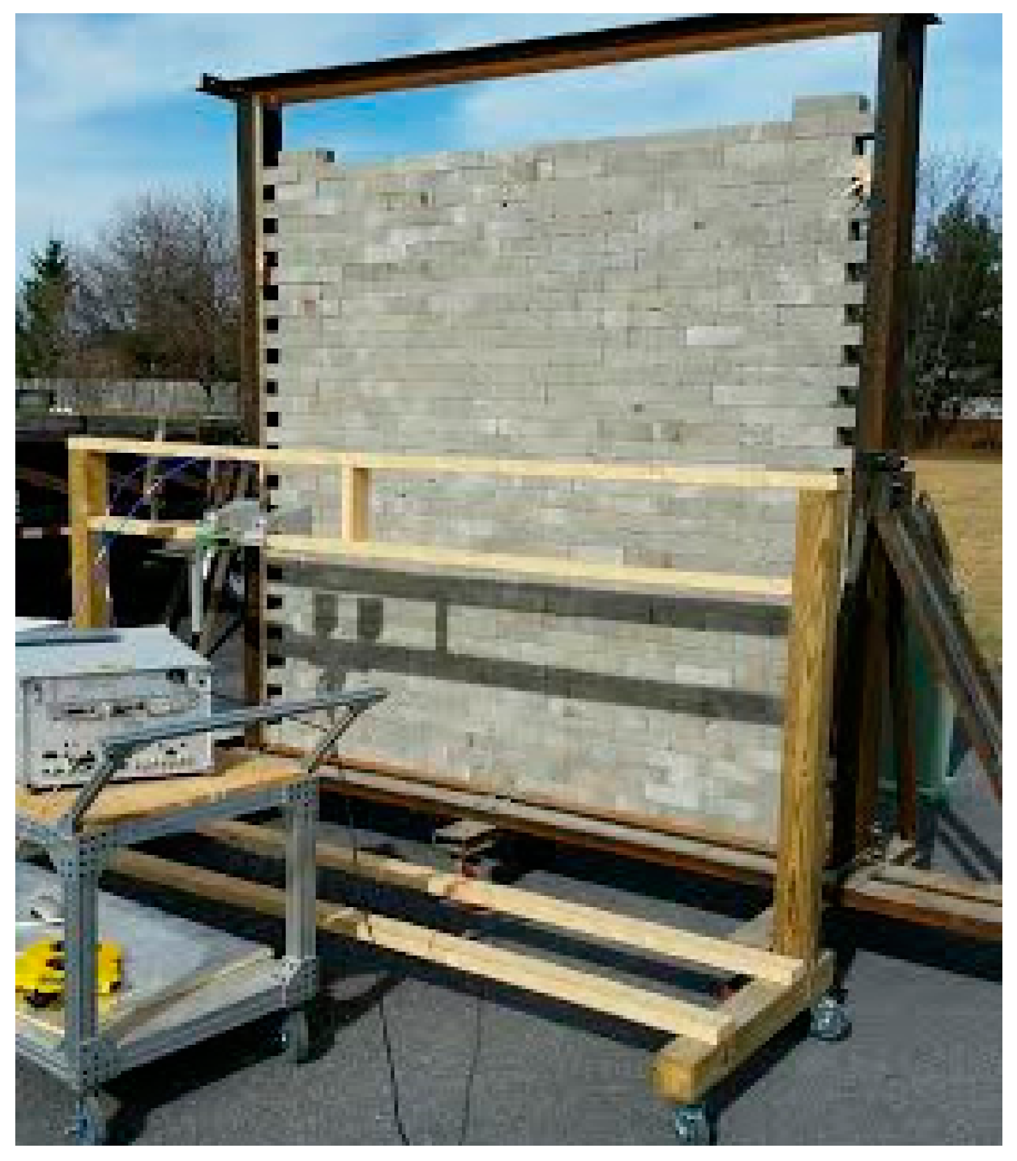
Figure 3.
Photograph showing the cart with the horn antennas mounted and the wall behind which the targets were located.
Figure 3.
Photograph showing the cart with the horn antennas mounted and the wall behind which the targets were located.

Figure 4.
Range migration algorithm block diagram.

Figure 5.
Images of corner reflector through wall at 3.96 m (13 feet) down-range centered azimuthally over 10–50 dB image dynamic range: (a) 10 dB; (b) 20 dB; (c) 30 dB; (d) 40 dB; (e) 50 dB.
Figure 5.
Images of corner reflector through wall at 3.96 m (13 feet) down-range centered azimuthally over 10–50 dB image dynamic range: (a) 10 dB; (b) 20 dB; (c) 30 dB; (d) 40 dB; (e) 50 dB.

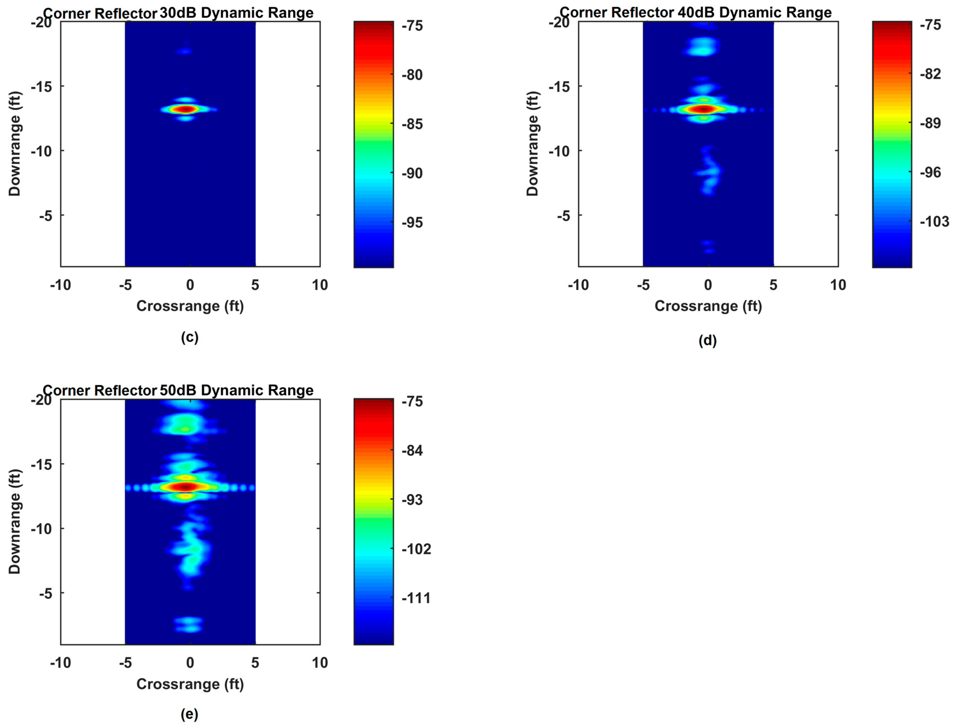
Figure 6.
Images of corner reflector through wall at 3.96 m (13 feet) with varying window and truncation application: (a) No truncation, no window; (b) No truncation, with window; (c) Truncation, no window; (d) Truncation first, then window; (e) Window first, then truncation.
Figure 6.
Images of corner reflector through wall at 3.96 m (13 feet) with varying window and truncation application: (a) No truncation, no window; (b) No truncation, with window; (c) Truncation, no window; (d) Truncation first, then window; (e) Window first, then truncation.
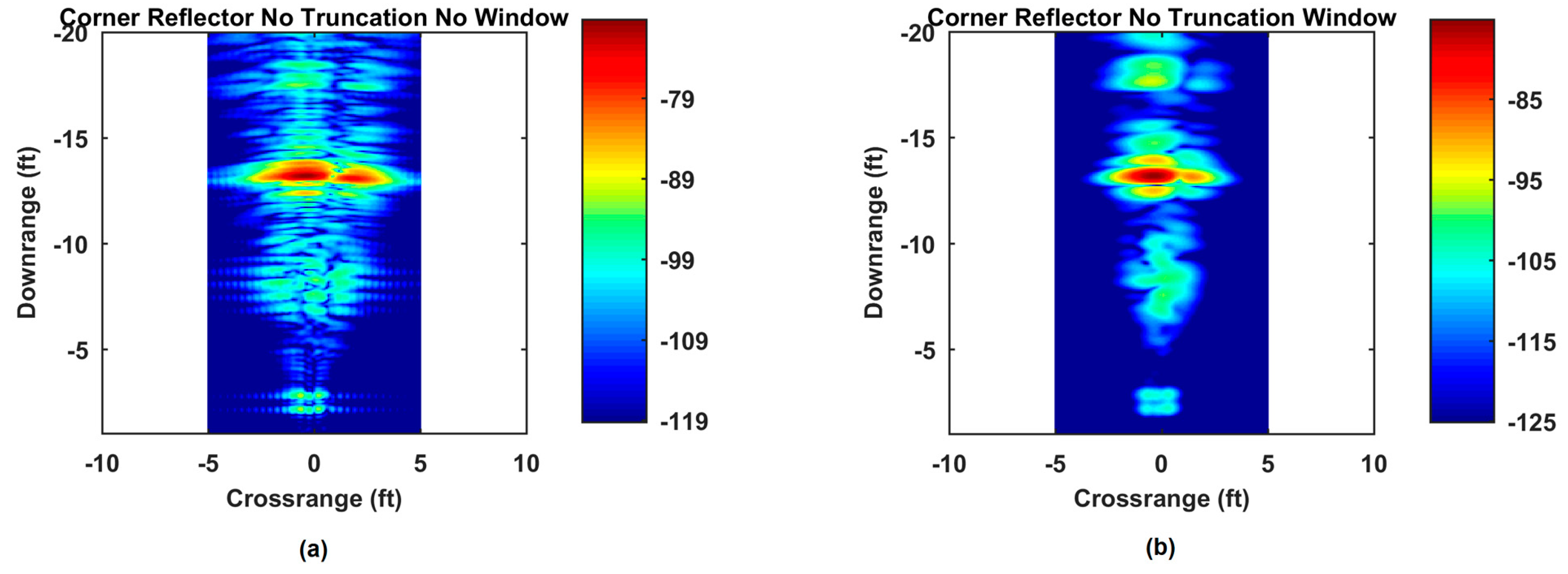

Figure 7.
Simplified multi-view scenario.
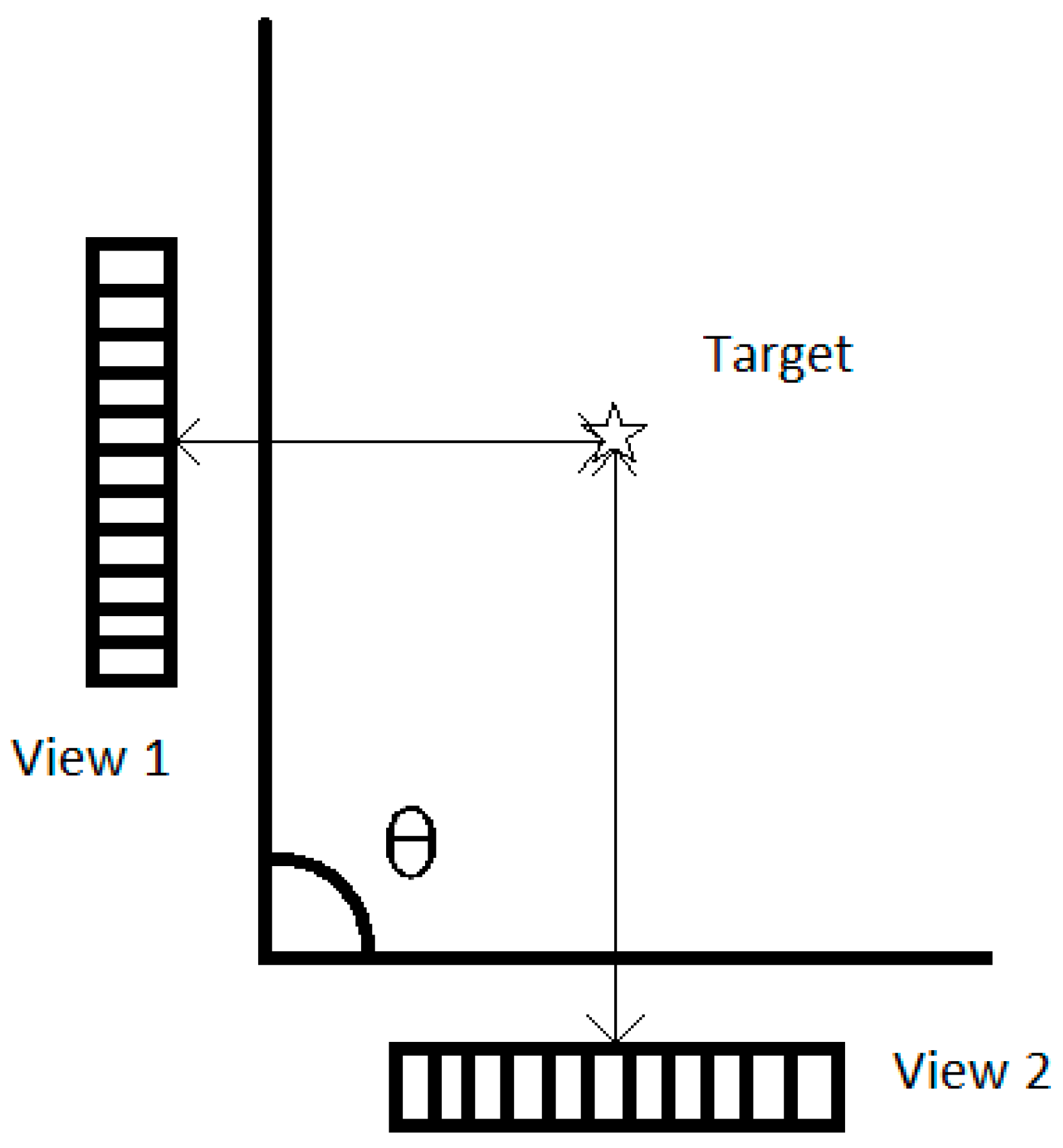
Figure 8.
Images of a single target 2.13 m (7 feet) down-range over 5–25 dB image dynamic range: (a) 5 dB; (b) 10 dB; (c) 15 dB; (d) 20 dB; (e) 25 dB.
Figure 8.
Images of a single target 2.13 m (7 feet) down-range over 5–25 dB image dynamic range: (a) 5 dB; (b) 10 dB; (c) 15 dB; (d) 20 dB; (e) 25 dB.
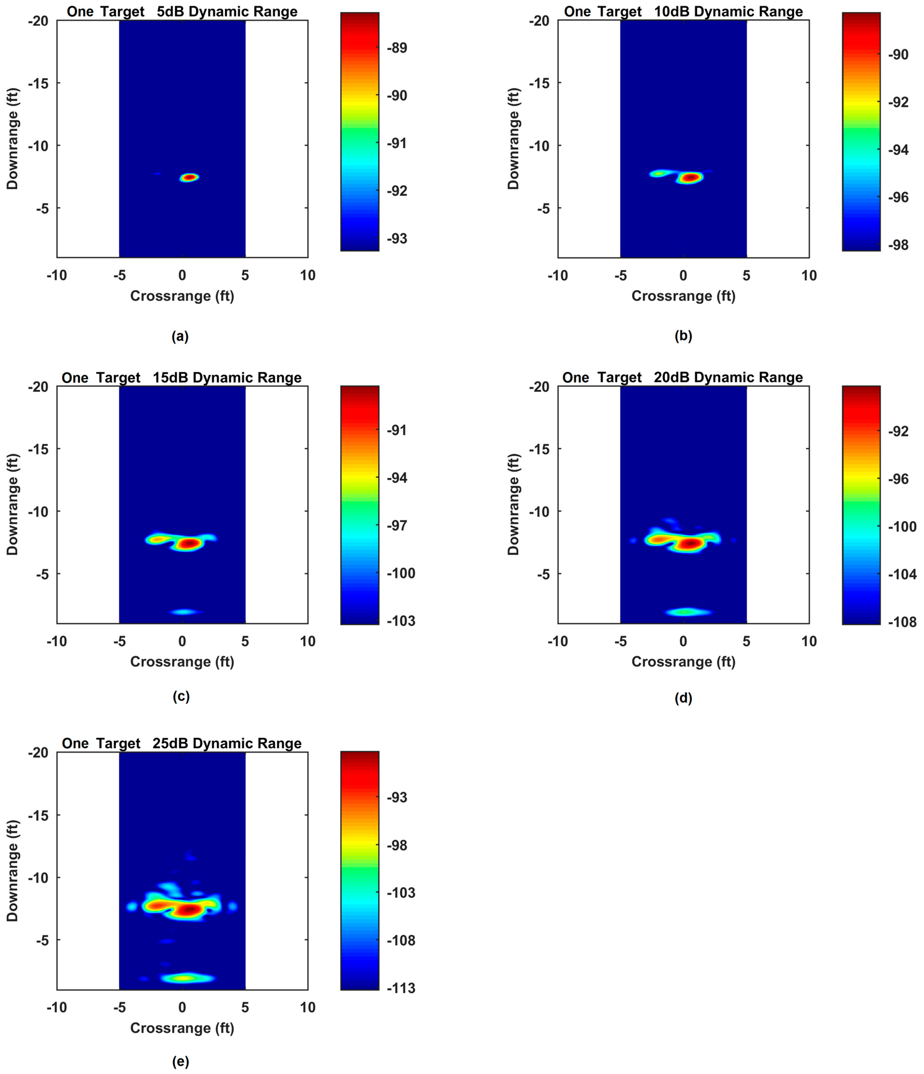
Figure 9.
Images of a single target 3.96 m (13 feet) down-range over 5–25 dB image dynamic range: (a) 5 dB; (b) 10 dB; (c) 15 dB; (d) 20 dB; (e) 25 dB.
Figure 9.
Images of a single target 3.96 m (13 feet) down-range over 5–25 dB image dynamic range: (a) 5 dB; (b) 10 dB; (c) 15 dB; (d) 20 dB; (e) 25 dB.

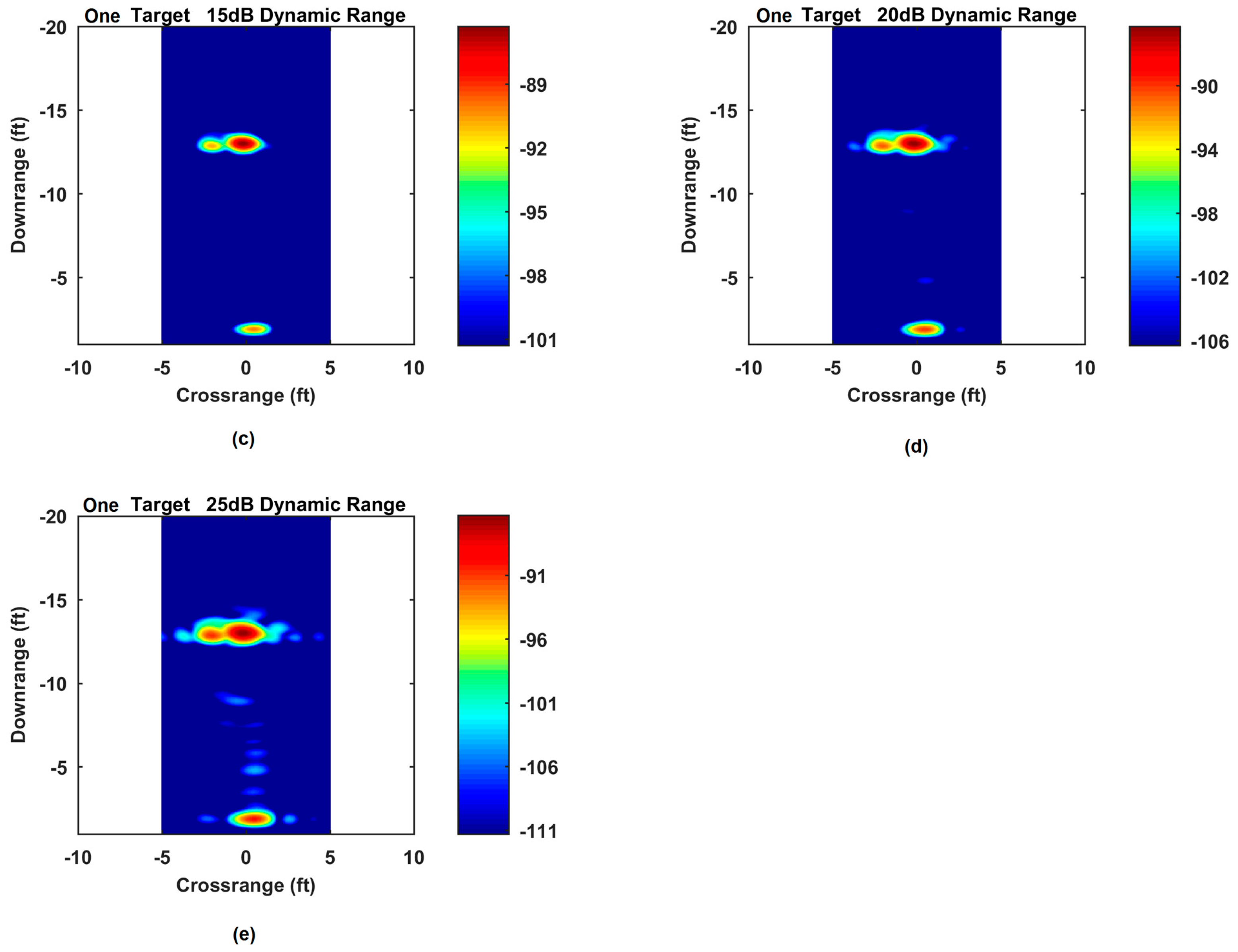
Figure 10.
Images of multi-target View 1 over 5–25 dB image dynamic range: (a) 5 dB; (b) 10 dB; (c) 15 dB; (d) 20 dB; (e) 25 dB.
Figure 10.
Images of multi-target View 1 over 5–25 dB image dynamic range: (a) 5 dB; (b) 10 dB; (c) 15 dB; (d) 20 dB; (e) 25 dB.
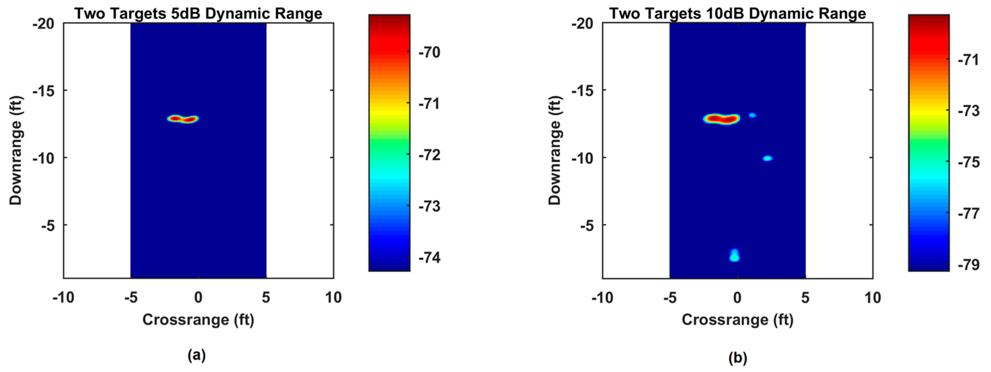

Figure 11.
Images of multi-target View 2 over 5–25 dB image dynamic range: (a) 5 dB; (b) 10 dB; (c) 15 dB; (d) 20 dB; (e) 25 dB.
Figure 11.
Images of multi-target View 2 over 5–25 dB image dynamic range: (a) 5 dB; (b) 10 dB; (c) 15 dB; (d) 20 dB; (e) 25 dB.

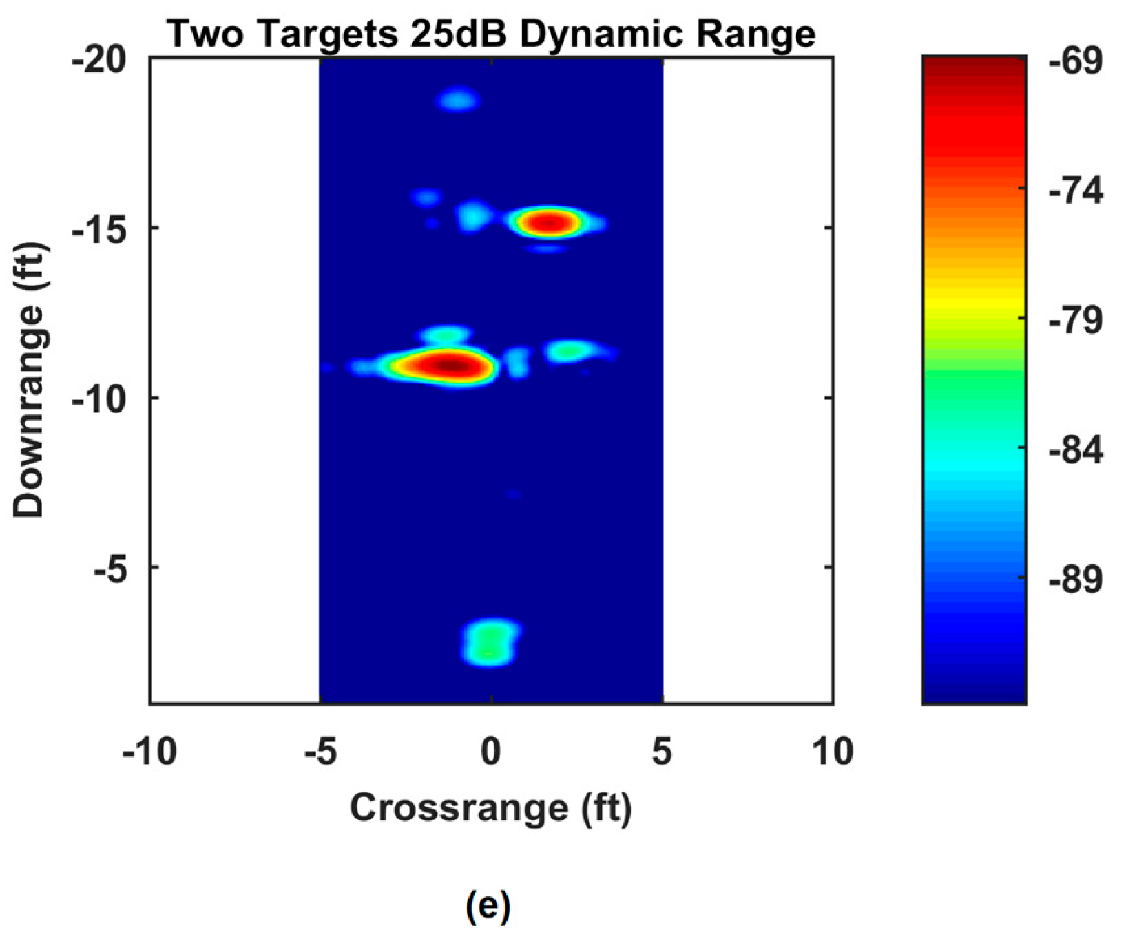
Figure 12.
Fused images of a single target over 5–25 dB image dynamic range: (a) 5 dB; (b) 10 dB; (c) 15 dB; (d) 20 dB; (e) 25 dB.
Figure 12.
Fused images of a single target over 5–25 dB image dynamic range: (a) 5 dB; (b) 10 dB; (c) 15 dB; (d) 20 dB; (e) 25 dB.


Figure 13.
Fused images of a single target over 30–50 dB image dynamic range: (a) 30 dB; (b) 35 dB; (c) 40 dB; (d) 45 dB; (e) 50 dB.
Figure 13.
Fused images of a single target over 30–50 dB image dynamic range: (a) 30 dB; (b) 35 dB; (c) 40 dB; (d) 45 dB; (e) 50 dB.
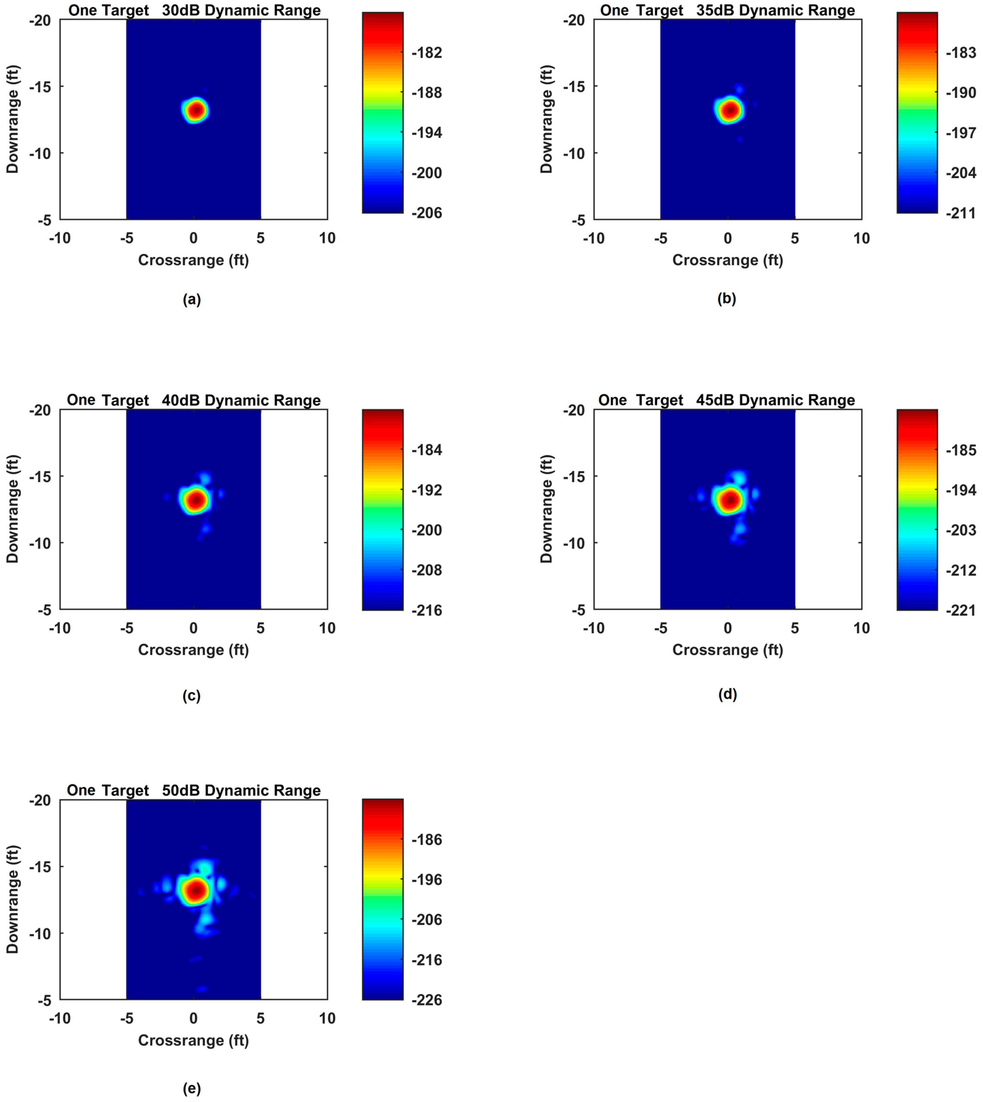
Figure 14.
Fused images of multiple targets over 5–25 dB image dynamic range: (a) 5 dB; (b) 10 dB; (c) 15 dB; (d) 20 dB; (e) 25 dB.
Figure 14.
Fused images of multiple targets over 5–25 dB image dynamic range: (a) 5 dB; (b) 10 dB; (c) 15 dB; (d) 20 dB; (e) 25 dB.

Figure 15.
Fused images of multiple targets over 30–50 dB image dynamic range: (a) 30 dB; (b) 35 dB; (c) 40 dB; (d) 45 dB; (e) 50 dB.
Figure 15.
Fused images of multiple targets over 30–50 dB image dynamic range: (a) 30 dB; (b) 35 dB; (c) 40 dB; (d) 45 dB; (e) 50 dB.

Figure 16.
Architecture of the two-dimensional wavelet transform (from [57]).
Figure 16.
Architecture of the two-dimensional wavelet transform (from [57]).
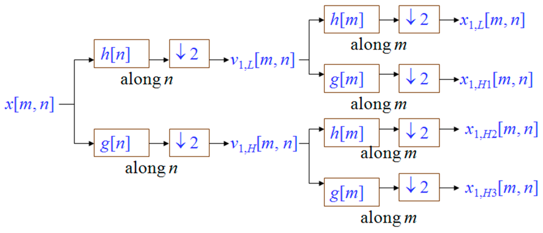
Figure 17.
Images of a single target 3.96 m (13 feet) down-range over 5–25 dB image dynamic range using SVD: (a) 5 dB; (b) 10 dB; (c) 15 dB; (d) 20 dB; (e) 25 dB.
Figure 17.
Images of a single target 3.96 m (13 feet) down-range over 5–25 dB image dynamic range using SVD: (a) 5 dB; (b) 10 dB; (c) 15 dB; (d) 20 dB; (e) 25 dB.

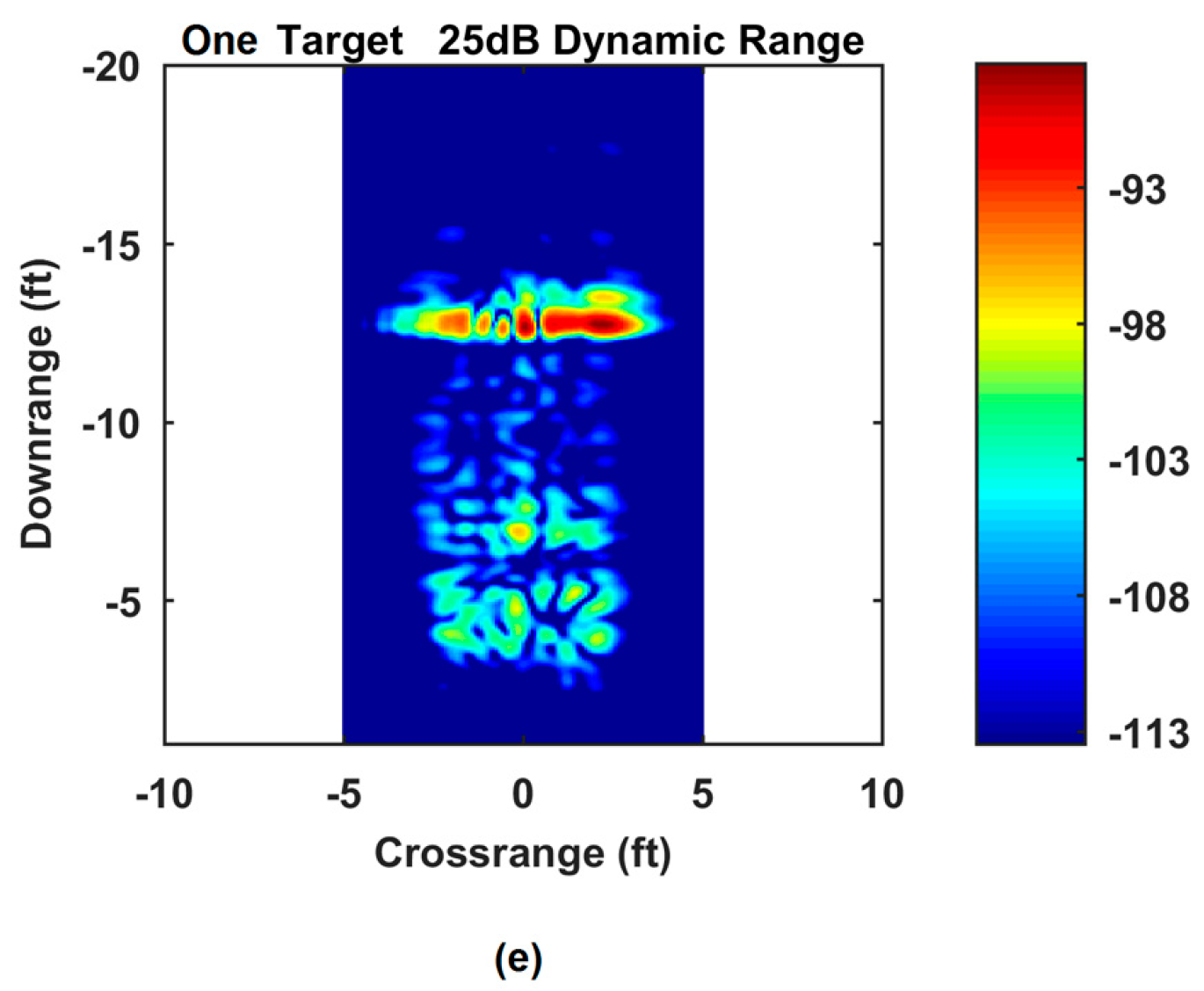
Figure 18.
Images of a multiple targets at 3.35 m (11 feet) and 4.57 m (15 feet) down-range over 5–25 dB image dynamic range using SVD: (a) 5 dB; (b) 10 dB; (c) 15 dB; (d) 20 dB; (e) 25 dB.
Figure 18.
Images of a multiple targets at 3.35 m (11 feet) and 4.57 m (15 feet) down-range over 5–25 dB image dynamic range using SVD: (a) 5 dB; (b) 10 dB; (c) 15 dB; (d) 20 dB; (e) 25 dB.
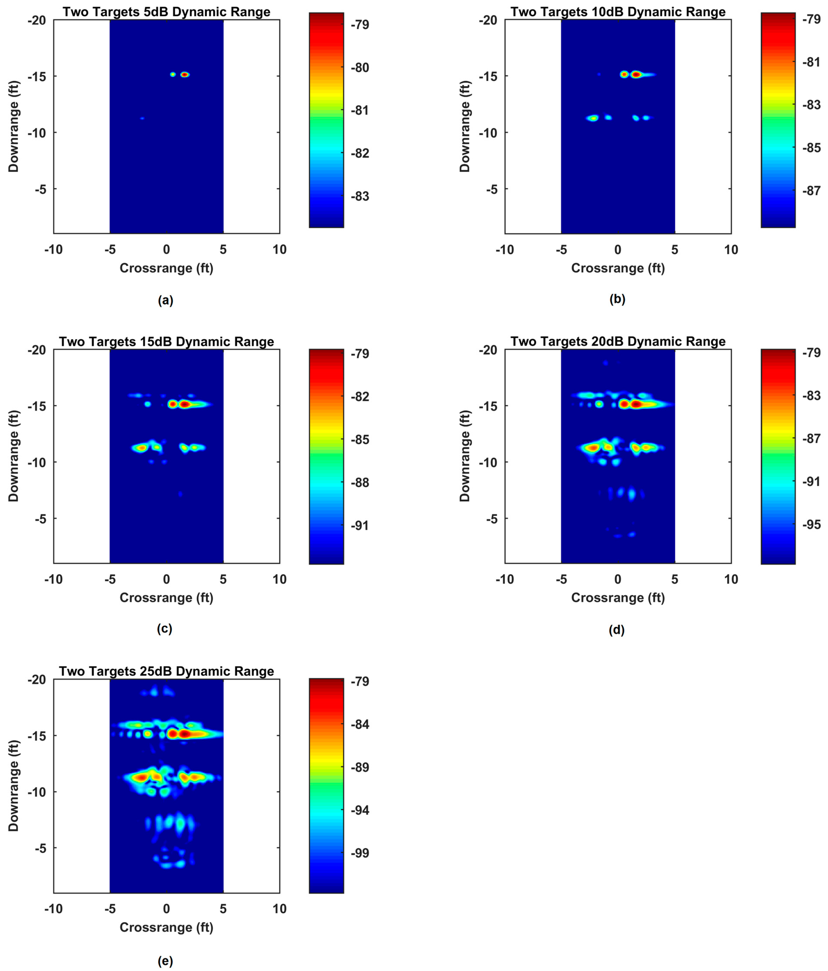
Figure 19.
Images of a single target 2.13 m (7 feet) down-range over 5–50 dB image dynamic range using wavelet-SVD: (a) 5 dB; (b) 10 dB; (c) 15 dB; (d) 20 dB; (e) 25 dB; (f) 50 dB.
Figure 19.
Images of a single target 2.13 m (7 feet) down-range over 5–50 dB image dynamic range using wavelet-SVD: (a) 5 dB; (b) 10 dB; (c) 15 dB; (d) 20 dB; (e) 25 dB; (f) 50 dB.

Figure 20.
Images of a multiple targets at 3.35 m (11 feet) and 4.57 m (15 feet) down-range over 5–50 dB image dynamic range using wavelet-SVD: (a) 5 dB; (b) 10 dB; (c) 15 dB; (d) 20 dB; (e) 25 dB; (f) 50 dB.
Figure 20.
Images of a multiple targets at 3.35 m (11 feet) and 4.57 m (15 feet) down-range over 5–50 dB image dynamic range using wavelet-SVD: (a) 5 dB; (b) 10 dB; (c) 15 dB; (d) 20 dB; (e) 25 dB; (f) 50 dB.


Table 1.
Comparison of processing methods.
| Method | TCR (dB) |
|---|---|
| No windowing and no truncation | 43.76 |
| No truncation and windowing | 49.22 |
| Truncation and no windowing | 48.89 |
| Truncation and windowing | 50.39 |
Table 2.
Comparison of single target 2-wall case.
| Method | TCR (dB) |
|---|---|
| Background subtraction Wall 1 | 40.99 |
| Background subtraction Wall 2 | 38.87 |
| Image fusion | 61.10 |
Table 3.
Comparison of multiple target 2-wall case.
| Method | TCR (dB) |
|---|---|
| Background subtraction Wall 1 | 44.12 |
| Background subtraction Wall 2 | 44.49 |
| Image fusion | 51.36 |
Table 4.
Comparison of wavelet and SVD approaches.
| Method | TCR (dB) |
|---|---|
| Single target SVD | 26.79 |
| Multiple target SVD | 31.70 |
| Single target wavelet | 45.04 |
| Multiple target wavelet | 47.53 |
© 2017 by the authors. Licensee MDPI, Basel, Switzerland. This article is an open access article distributed under the terms and conditions of the Creative Commons Attribution (CC BY) license (http://creativecommons.org/licenses/by/4.0/).
Share and Cite
MDPI and ACS Style
Narayanan, R.M.; Gebhardt, E.T.; Broderick, S.P. Through-Wall Single and Multiple Target Imaging Using MIMO Radar. Electronics 2017, 6, 70. https://doi.org/10.3390/electronics6040070
AMA Style
Narayanan RM, Gebhardt ET, Broderick SP. Through-Wall Single and Multiple Target Imaging Using MIMO Radar. Electronics. 2017; 6(4):70. https://doi.org/10.3390/electronics6040070
Chicago/Turabian StyleNarayanan, Ram M., Evan T. Gebhardt, and Sean P. Broderick. 2017. "Through-Wall Single and Multiple Target Imaging Using MIMO Radar" Electronics 6, no. 4: 70. https://doi.org/10.3390/electronics6040070
Note that from the first issue of 2016, this journal uses article numbers instead of page numbers. See further details here.