A Comparative Reliability Study of Three Fundamental Multilevel Inverters Using Two Different Approaches

Abstract

The reliability of power electronic devices and components is very important to manufacturers. In recent years, many researchers have conducted reliability assessments of power electronic devices, yet the reliability of numerous circuits used widely has not been evaluated. This paper presents a comprehensive reliability evaluation of fundamental multilevel inverters. The reliability of the multilevel inverters is analyzed by calculating the mean time to failure for each component. The calculation was performed by two methods (approximate and exact) to achieve better comparisons. The approximate method is similar to the parts count method used in MIL-HDBK-217 reliability standard, and the exact method exhibits the parts stress method. In the exact method, due to the direct relationship between component failure and temperature, we used Matlab Simulink to determine power losses in diodes and switches taking into account the temperature factor. The results determined by the approximate method showed that the three-level cascade H-bridge was the most reliable of the inverters considered. Although the exact method validates those results, and shows that cascade H-bridge (CHB) had a longer lifespan, but the calculated values are different. Therefore, using different approaches for evaluating reliability results in different outcomes.

1. Introduction

In the recent years, reduction of fossil fuel resources has drawn much attention to the importance of renewable energies. The use of renewable sources such as solar panels and wind turbines requires extensive use of power electronic devices and the popularity of renewable energies, particularly wind and solar energy is growing by the day. Photovoltaic systems are considered one of the best renewable energy sources both on small and large scales [1]. The first solar cells were made in 1883 [2] and, today, photovoltaic sources are used in different sectors, such as battery chargers, water pumps, household electricity generation, satellites, etc. [3]. One of the main challenges facing the use of renewable energies is the ever changing level of generated power. Of course, the power quality is also one of the main concerns in this regard, which becomes more important with the significant increase in the number of electronic devices [4].

Solar panels generate a DC voltage, so using solar energy requires an inverter to convert the DC voltage to AC. Today, industry needs equipment with higher power, so direct connection of AC voltage generated by renewable source to the grid with medium voltage level is essential. Therefore, multilevel inverters have been introduced to work with higher voltages and also to improve the output voltage [5].

There are different topologies and control methods for multilevel inverters. In general, multilevel inverters can be divided into two categories: fundamental and modern. There are three fundamental topologies for multilevel inverters [5,6,7,8,9]:

• diode-clamped or neutral-clamped (NPC)
• capacitor-clamped or flying capacitor (FC)
• cascade H-bridge (CHB)

The NPC inverter was introduced in the 1990s, and it has been widely used in FACTS (flexible alternating current transmission system) and industrial drives. The FC inverter with a three-phase topology was presented for the first time in the early 1980s. The clamping capacitors provide the smooth switching frequency ripple voltage, but their capacity is small. However, increasing the number of voltage levels leads to some problematic issues: namely, thermal, low-inductance, and insulation designing. CHB multilevel inverters have been used in various practical applications such as broadcasting amplifiers, industrial drives, and STATCOMs (static synchronous compensators). The primary disadvantage of this inverter is the presence of an individual power supply for each H-bridge cell [10]. In this paper, we used these three mentioned inverters though the three-level scheme, and the circuit diagram of one leg of these inverters is shown in Figure 1.

Although the fundamental inverters have found a great application in different industries, there are many things still unknown about these topologies, because improvements of other types of converters remain unresolved. In the recent decades, some new topologies have been proposed to improve the performance, increase reliability and reduce the number of circuit elements. Using mixed-level hybrid multilevel cells by replacing H-bridge with diode-clamped and capacitor-clamped gives much better results, and can generate the appropriate number of levels by reducing the number of independent DC sources [5]. Soft-switched inverters are another type of modern inverter. The purpose of the soft-switched inverters is to reduce switching losses and increase converter efficiency. Implementing the soft switching system in the cascade inverter is not different from the conventional two-level inverter structure because each inverter cell is a two-level circuit [5]. However, implementing soft switching circuit for diode-clamped and capacitor-clamped structures will be different [11,12,13].

Many of the proposed topologies have been introduced to merely reduce the number of independent voltage sources and switches. In Reference [14], instead of using two 6-switch inverters for feeding two engines, a 5-leg 10-switch inverter is used for simultaneous feeding of two engines, which means that two switches have been removed from the design. Kominami and Fujimoto introduced a novel 3-leg 9-switch inverter for simultaneous and independent feeding of two three-phase loads, which means using one switch lesser than the previous topology [15]. Generally, reducing the number of switches and elements in power electronic circuits increases the reliability of the inverter. As previously mentioned, the solar cells are also used for providing electrical power for satellites. In Reference [2], 6 Photovoltaic (PV) modules installed on an orbital satellite were studied to estimate the most efficient way of receiving power. In a satellite feed system, lifetime of the inverter and PV module is one of the most important issues. Higher inverter reliability means higher operational lifespan. Of course, most PV module manufacturers guarantee 25 years lifespan ending up with around 25% initial efficiency [16]. Therefore, it is necessary to pay more attention to the issue of inverter reliability (especially for multilevel inverters which are considered as the new generation of inverters).

This paper presents a comprehensive review on the principle of reliability and assessment of multilevel inverter in terms of reliability. Two approximate and exact method are used to determine reliability of multilevel inverters. The approximate method is based on the parts count method and summing the reference failure rates for each component. The exact method exhibits a parts stress method used to evaluate the reliability of inverters. In this paper, for the first time, reliability of fundamental multilevel inverters is determined using an exact method and considering all conditions.

The remainder of this paper is organized as follows: Section 2 introduces the fundamental principle of reliability and different approaches. Section 3 proposes the approximate and exact method to assess the reliability, and in Section 4, a comprehensive reliability evaluation is presented using two approaches for three multilevel inverters of CHB, FC, and NPC. Moreover, the effect of series redundancy is shown in this section. Finally, Section 5 presents the conclusions.

2. Fundamental Principle of Reliability

Extracting the highest possible efficiency from each device has always been the goal of manufacturers. In power converters, this optimal utilization includes high output quality, longer lifespan, less energy consumption, etc. In fact, having a converter with longer lifespan means having a converter with more reliability. Reliability shows the probability of system failure at a given time [17]. The reliability of a system depends on different factors; therefore, to assess that system, it must be divided into smaller parts and reliability of each part then must be investigated. The reliability is usually assessed from various aspects. To determine the reliability of a system, researchers often use indices such as failure rate, mean time to failure (MTTF) and mean time to repair (MTTR) and Availability [18]. Therefore to determine the reliability of a system, first it is necessary to define the basic concepts.

2.1. Reliability

Reliability is defined as "the ability of an item to perform the requested function under the stated conditions over a specified time period" and is often measured as failure probability or failure frequency [19]. Most systems include three categories of reliability. These three categories include [20]:

• Software reliability
• Hardware reliability
• Human reliability

In studies covering the concept of reliability, the reliability of a system is usually considered independent from time, which for industrial products should be in the warranty period [18]. Failure over time can be shown in three different time periods. The first period is the learning phase, where work failure decreases with the passage of time. Length of this period can vary from several minutes to several hours. The second period is the failure consolidation phase which shows that after the learning phase, failure does not change by the passage of time; length of this period is random. The third period, is the fatigue phase, where the failure rate increases with the increase of time. By combining these three periods over a single time period, combined failure graph can be obtained [20].

This combined graph can be shown in the form of hazard function, in which case it is called the bathtub curve graph (Figure 2). Similar to combined graph, this graph consists of three parts [21]:

• The early failure or burn-in period, where the hazard function decreases with time.
• The random failure or useful life period, where the hazard function is constant.
• The wear-out period, where the hazard function increases.

In recent decades, many definitions have been proposed for the reliability concept. For instance, The Oxford dictionary defines reliability as “the quality of being reliable, that may be relied upon; in which reliance or confidence may be put; trustworthy, safe, sure” [22]. In 1987, Hammersley presented another definition of reliability: “Reliability is the agreement between two efforts to measure the same trait through maximally similar methods” [23]. There is a lack of comprehensive study in the literature on the reliability of power electronic converters. In References [18,24], an overall assessment on power electronic system reliability has been conducted. In Reference [25], authors have used condition monitoring in order to estimate reliability. In Reference [26], the evaluation of reliability for a DC-DC Boost converter has been conducted with a reliability improvement approach. The reliability evaluation of modular multilevel converters (MMCs) as a very important topology must be noted. Rashidi-Rad et al. presented a reliability evaluation of modular multilevel inverters with half and full-bridge cells based on two different methods [27]. Their research showed that the modular inverters which utilized half-bridge cells performed better in terms of reliability, in comparison to the full-bridge modular inverters.

Nevertheless, reliability evaluations and finding ways to improve them are important. For this reason, there are different experimental and practical examples on the reliability of power electronic applications. Anurag et al. analyzed the effect of reactive power injections by inverters used in photovoltaic applications on their thermal operation and component reliability [28]. The authors suggested that regulations should be made by setting a limit on reactive power injections by PV inverters. Isidori et al. investigated the reliability of a three-level back-to-back converter for a 10 MW wind turbine based on the semiconductors thermal behavior [29]. It was concluded that 60° discontinuous pulse width modulation shows more appropriate thermal performance. Additionally, some experimental researches have been conducted for the reliability of components extensively used in power electronic devices. For instance, a detailed study of the reliability of DC-link capacitors is presented in Reference [30].

Considering the wide use of semiconductor devices in power electronics, assessing their reliability is essential and imperative [31,32]. For example, the reliability of IGBTs has been assessed and soldering condition has been identified as an important factor in the reliability of the IGBT module.

2.2. Failure

Failure occurs when the system stops to perform the requested function, for any reason. So, failure-free operation time is generally a random variable, which can be long or short. Failure can be divided into two categories: sudden and gradual. The sudden failure is considered as cataleptic failure and gradual failure is considered as degradation failure [33].

2.3. Failure rate

Failure rate has an important role in determination of system reliability. The failure rate function can determine the probability of failure over a specified time period. It can be defined as the failure probability per time unit in the period of [t, t+Δt], when there has been no failure before t. Failure rate can be obtained as follows [34]:

$$Failure rate= \frac{P\left(t\le T\le t+\Delta t|T>t\right)}{\Delta t}=\frac{P\left(t\le T\le t+\Delta t\right)}{\Delta t.P(T>t)}$$

(1)

where P(t ≤ T ≤ t + ∆t) is the failure probability of T in the time period of [t,t+Δt]. This probability can be linked with CDF(f(t)) and PDF(f(t)) of the failure density function [34]:

$$P\left(t\le T\le t+\Delta t\right)=f\left(t\right)\Delta t=F\left(t+\Delta t\right)-F\left(t\right)$$

(2)

If we show the failure probability by failure distribution, the probability of failure non-occurrence over a specified time period is obtained by the reliability probability distribution which is the difference between the sum of all probabilities (equal to 1) and the failure probability. Therefore, we can obtain the reliability function of the constant hazard section by the following equation [35]:

$$R\left(t\right)=1-F\left(t\right)$$

(3)

In fact, this function is the P(T > t) function. Thus, the system reliability can be obtained directly from the failure density function. The evaluation of reliability is only possible by knowing the reliability of components. Reliability of components is generally obtained by two failure distribution functions: Exponential and Weibull [34,35].

Δt value is usually very small and close to zero. Thus, by assigning a small value to Δt in the previous failure rate equation, we obtain the failure rate function equation [36]:

$$z\left(t\right)=\underset{\Delta t\to 0}{\lim }\frac{F\left(t+\Delta t\right)-F\left(t\right)}{\Delta t.R\left(t\right)}=f\left(t\right)/R\left(t\right)$$

(4)

Failure rate is also shown by λ. Using the Exponential distribution, the probability distribution function is obtained as a combination of failure rates:

$$f\left(t,\mathsf{\lambda }\right)={\mathsf{\lambda }\mathrm{e}}^{-\mathsf{\lambda }t}$$

(5)

The reliability function is as follows [35]:

$$R\left(t,\mathsf{\lambda }\right)={\mathrm{e}}^{-\mathsf{\lambda }t}$$

(6)

It should be noted that Equation (6) is true for the hazard fixed period. The failure rate estimated by the average number of failures per unit time is expressed in the form of failure in time (FIT) [18]:

$$1 \text{FIT}={10}^{-9} \text{failure}/\text{hour}$$

(7)

Generally, using bathtub graph for modeling the failure rate function is a great tool for assessing the reliability of the system. In recent years, there have been many studies covering subject of failure rate function. In Reference [37], 17 different functions have been introduced to present the bathtub shape which has made this article a good reference for failure rate function models. Carrascoa et al. [38], have proposed a modified four-parameter Weibull distribution function for modeling the bathtub graph. The advantage of this distribution function is its ability to perform monotone modeling as well as non-monotone modeling. In Reference [39], the generalized two-parameter Weibull distribution function has been presented, and the authors have stated that proper results can be achieved by selecting the appropriate parameter values for the proposed distribution function. In Reference [40], also similar to other mentioned articles, a generalized three-parameter distribution function has been used to obtain the failure rate function; the results of that article showed that the introduced distribution function is more flexible than some other proposed functions.

2.4. Mean Time to Failure

Mean time to failure (MTTF) is the average time before the first failure of a component or device after it starts to work. This failure is such that the device is no longer able to continue its normal functions. MTTF is usually estimated in hours or thousand hours and is often listed among the parts specifications. When MTTF of a device is reported as one hundred thousand hours, it means that the first failure disrupting the device functioning is expected to occurs after this time period. Here, two important points should be mentioned.

1. This time is only a guarantee. There is no guarantee that the device will not fail after a few hours of work or that it will definitely fail after one hundred thousand hours and will not work much longer than that.

2. This time is the actual time that device functions. For example, one hundred thousand hours is equal to about 11 years and 5 months. However, if device is used 8 h a day, this period becomes actually 3 times longer, about 34 years, because device has not been operating 24 h a day.

MTTF is expressed by reliability function, and is as below:

$$MTTF={{\displaystyle \int }}_0^{+\infty }R\left(t\right)dt$$

(8)

where reliability function must be obtained by e^−λt. Thus, the more simplified form of MTTF is as follows [18,34,35,36]:

$$MTTF=1/\lambda$$

(9)

As seen from Equation (8), the value of MTTF has a direct relationship with the reliability function, so MTTF value changes with different assumptions for reliability function. For example, in Reference [40], reliability function, which is expressed in terms of generalized Weibull function, is in a different form. Several studies have been conducted on MTTF concept. Heidelberger et al. presented a good numerical method to calculate the MTTF in a Markovian model [41].

MTTF is an incomplete statistical parameter, and it is one of the main limitations of MTTF, so that it does not properly show the failure behavior, especially when failure mechanism has not a constant failure rate [42]. In Reference [43], nTTF (the time to failure of n% of the population) have been studied. nTTF reports on failure rate are more accurate than MTTF, but it is more difficult to use because it requires the distribution of failure times [43].

2.5. Mean Time to Repair

MTTR is the average time spent to repair a failed device and its value is dependent on maintenance conditions [17]. If we assume the time required to repair System x has a gamma distribution with parameters μ and β, then MTTR can be obtained by [44]:

$$MTTR={{\displaystyle \int }}_0^{+\infty }xN\left(x\right)dx=\frac{\beta }{\mu }$$

(10)

where N(x) is the gamma distribution function. By assigning 1 to β, gamma distribution becomes equivalent to exponential distribution, therefore summarized MTTR value can be shown by 1/μ. MTTR is very difficult to calculate and it is usually determined empirically by studying the previous repairs [45].

2.6. Mean Time between Failures

Mean time between failures (MTBF) is one of the most important quantitative parameters that can help us achieve preventive maintenance as well as reliability. MTBF is the average time between two successive failures. In some cases, none of the MTBF definitions can properly describe the system reliability; for example, when the distribution function is not exponential, it is practically impossible for MTBF to predict the time to failure [46]; but in systems with random failures and emergencies that may include a wide range of failures and components, MTBF can be a good measure to predict emergency failures. In References [47,48], authors have acknowledged MTBF as a good measure have stated that it provides an appropriate combination of MTTR and MTTF measures.

MTBF can be obtained from the following equation [49]:

$$MTBF=MTTF+MTTR$$

(11)

In Reference [50], condition-based fault tree analysis (CBFTA) has been used to improve the accuracy of MTBF measurement. In fact, CBFTA is a tool for updating the values of system reliability and calculating these values accurately along with monitored system condition. The results show that using CBFTA improves the level of system reliability.

2.7. Availability and Average Availability

Availability is one of the most important measures of reliability and shows the probability of system being functional at a given time. Average Availability or Point Availability represents is the probability of functionality of requested component under given conditions during time period of t. Average Availability can be obtained from the following equation [18]:

$$A_{avg}=\frac{MTTF}{MTTF+MTTR}$$

(12)

Thus, Availability improves by increasing MTTF and reducing MTTR. Expressing A_avg as (MTBF-MTTR)/MTBF is usually avoided [33]. According to the authors of [51], increasing MTTF does not necessarily increase the value of Availability and Average Availability; also, Availability and Average Availability can be increased without changing MTTF.

3. Methodology

In recent decades, various procedures for estimating the reliability have been introduced by different organizations. The first of reliability estimation titled TR-1100 was published in 1956 in United States by Rome Air Development Center (RADC). This standard described the failure rate for electronic and computer parts [52]. After the publication of this standard, MIL-HDBK-217 was published as a handbook and became the most popular one in this field. After that different firms and organizations developed and improve their own reliability handbooks and software. Some of these procedures include:

• RAC’s PRISM [53]
• Telcordia SR-332 [54]
• SAE’s PREL [55]
• CNET's reliability prediction method [56]
• Siemens’ SN29500 standard [57]
• British Telecom’s HRD-4 [58]

In Reference [59], authors made a comparison between different methods available for estimating the reliability. Today, MIL-HDBK-217 handbook is still used as a reference for reliability estimation. It should be mentioned that MIL-HDBK-217 is a standard applied to military industry so it is very conservative compared to other standards. Moreover, the suitability of this standard compared to other ones has been proved because of its different and more factors which cover all aspects of reliability and influential items [60]. This handbook uses two methods called parts count and parts stress to estimate the reliability of system components at various stages of design [47,61].

Having the stress of electrical components and designed circuits, reliability can be predicted by using parts stress method. The parts count method requires less data, generally including information such as the number of parts, their quality level, and conditions of use. That is why parts stress methods usually yields more accurate results regarding system reliability [47]. The main difference between the parts stress and parts count methods is in how they calculate the system failure rate.

3.1. Approximate Method

As previously mentioned, there are two extensively used approaches for reliability assessments to calculate failure rates. The first method is parts count which is a simple way to estimate the reliability of a system. When there is no detailed system information, using this method is preferred. This method uses typical operating conditions called reference conditions to predict the failure rate under these conditions. However, it may be assumed that the device is not working under reference conditions, and the actual operating conditions will affect failure rates calculated from the parts count method. Therefore, this method can be considered as an approximate method. In this method, only the number of components is important, and the construction is not involved. Therefore, this method is typically based on quantitative analyses.

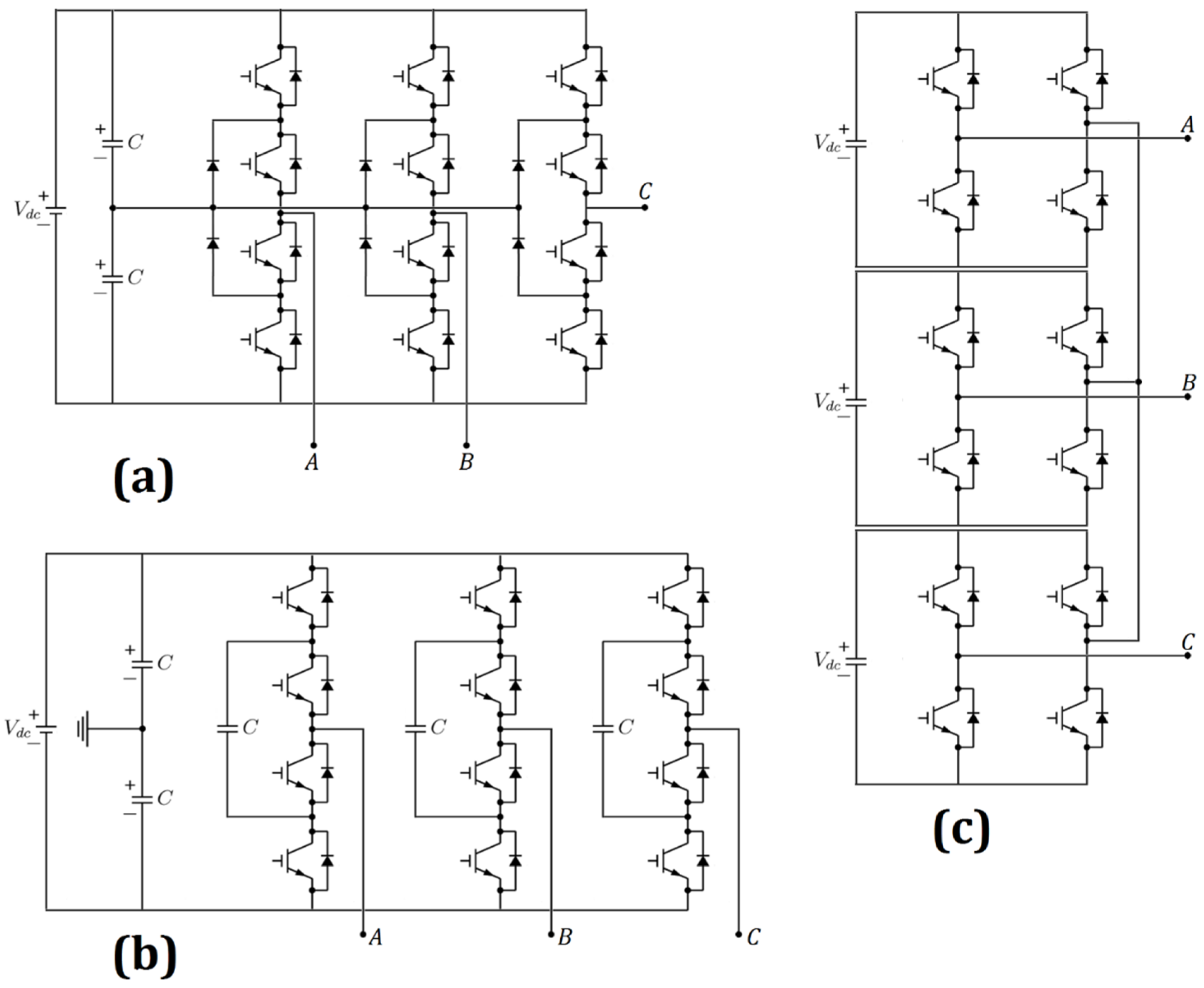
The approximate method used in this paper is similar to the method employed in Reference [62], which the reliability of three-level NPC and CHB inverter based on FIT has been studied. In that article, the voltage difference between circuit elements in properly compared. In this comparison, NPC has used IGBT’s with medium voltage and CHB has used low voltage. In this comparison, the quantities of components have been the center of focus. The results of that article have shown that in terms of reliability, NPC inverter is 4.5 times better than CHB inverter.

It is obviously clear that one of the factors required for the analysis using this method is the voltage level of investigated inverters. In fact, this method of comparison is the same as parts count method, where failure rates are estimated based on voltage values. In addition, the comparison has been made when inverters were connected to the drive. Therefore it is necessary to make a comparison individually and without drive.

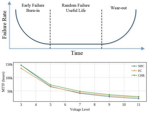
As mentioned above, we should find the voltage level of inverters in the first step. According to the authors of [62,63], the NPC, FC, and CHB inverters can be placed in the category of high, high, and low voltage IGBT switches. Based on this method, failure rate of diode has always been determined as 100 FIT, and failure rates of high voltage and low voltage IGBT have been determined as 400 FIT and 100 FIT, respectively. Additionally, failure rate of high voltage capacitor has been determined as 300 FIT and this parameter for low voltage capacitor has been determined as 400 FIT. The whole system failure rate can be determined by multiplying the diode, IGBT, and capacitors failure rate by their quantity, and summing all obtained values.

In general, the failure rate for a device under reference conditions can be expressed by:

$${\mathsf{\lambda }}_{SYSTEM}={\displaystyle \sum }_{i=1}^N{\mathsf{\lambda }}_{ref\left(i\right)}\times k$$

(13)

where k is the number of elements with the reference failure rate of λ_{ref (i)}, and N is the number of parts.

3.2. Exact Method

The exact method presents a scheme of parts stress method. Unlike the parts count method, parts stress method requires knowledge of the specific part’s stress levels and different operating conditions. In order to assess reliability of a system using this method, the various stresses on each part and accurate environment conditions are needed. These conditions can be shown by different pi factors in the failure rate equations. Number of various parameters in this method leads to a complexity in determining the failure rates, and although increases the accuracy. The total failure rate in the parts stress method can be calculated by summing all failure rates, similar to the parts count method. The following discussions will review the related relations of the exact method.

In MIL-HDBK-217 handbook, the failure rate of circuit components is calculated using an index called the base failure rate. Equation of base failure rate can be shown as below [64]:

$${\mathsf{\lambda }}_b=A.\exp \left(\frac{N_T}{273+T+\left(\Delta T\right)S}\right).\text{exp}{\left(\frac{273+T+\left(\Delta T\right)S}{T_M}\right)}^P$$

(14)

where A is the scaling factor of failure rate. N_T, T_M, and P are the shape parameters, T is the temperature, ΔT is the difference between maximum allowable temperature with no junction current and the maximum allowable temperature with full rated junction current or power, S is the stress ratio that can be calculated by the ratio of actual stress to rated stress.

Handbook MIL-HDBK-217 offers a combined approach to predict reliability so that the reliability of each part of the system is determined individually and as a whole. Form of this model is as follows [65]:

$${\mathsf{\lambda }}_p={\mathsf{\lambda }}_O{\mathsf{\pi }}_O+{\mathsf{\lambda }}_e{\mathsf{\pi }}_e+{\mathsf{\lambda }}_C{\mathsf{\pi }}_C+{\mathsf{\lambda }}_{Sj}{\mathsf{\pi }}_{Sj}+{\mathsf{\lambda }}_i$$

(15)

where λ_p is the predicted failure rate, λ_O is the failure rate from operational stresses, λ_e is the failure rate caused by environmental stresses, λ_C is the failure rate caused by temperature cycling stresses, λ_Sj is the failure rate caused by solder joints, λ_i is the failure rate caused by induced stresses, π_O is the operational factor, π_e is the environmental factor, π_C is the cycling factor, and π_Sj is the solder joints factor.

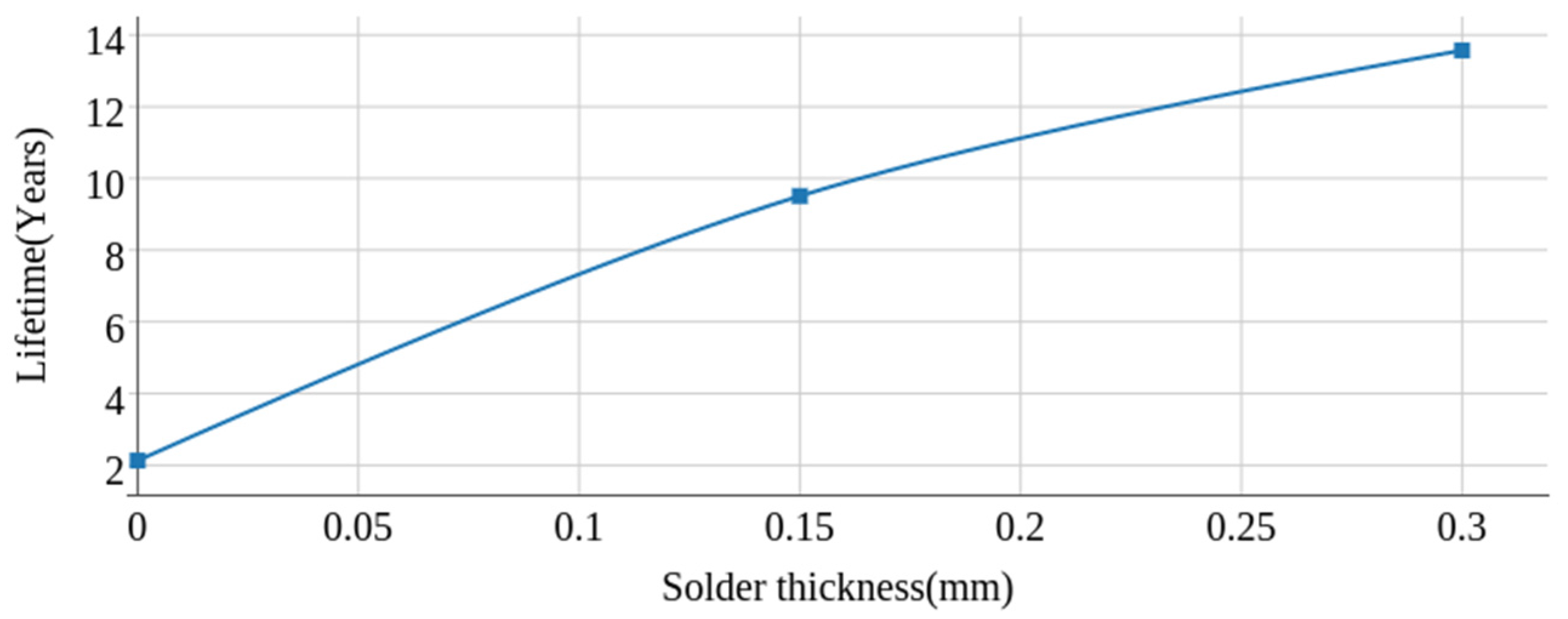
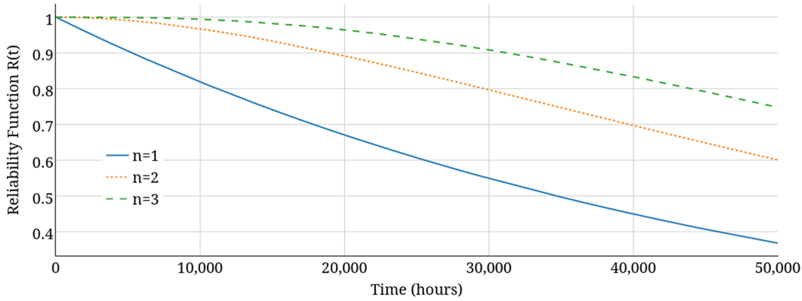
As the thickness of the solder increases, reliability also increases. Figure 3 shows the effect of solder joint on the reliability of an IGBT module; as can be seen, module lifetime increases with increasing thickness of solder [32]:

Recent articles about the reliability of electronic components (switches, diodes, capacitors and inductors) have presented specific relationships and equations for failure rate in each of these components. Considering to the components usually used in power electronic circuits, in this paper we express the failure rate for the following elements [26,47,66,67]:

$${\mathsf{\lambda }}_p\left(Capacitor\right)={\mathsf{\lambda }}_b{\mathsf{\pi }}_{CV}{\mathsf{\pi }}_Q{\mathsf{\pi }}_E$$

(16)

$${\mathsf{\lambda }}_p\left(Inductor-Transformer\right)={\mathsf{\lambda }}_b{\mathsf{\pi }}_C{\mathsf{\pi }}_Q{\mathsf{\pi }}_E$$

(17)

$${\mathsf{\lambda }}_p\left(Switch\right)={\mathsf{\lambda }}_b{\mathsf{\pi }}_T{\mathsf{\pi }}_A{\mathsf{\pi }}_Q{\mathsf{\pi }}_E$$

(18)

$${\mathsf{\lambda }}_p\left(Diode\right)={\mathsf{\lambda }}_b{\mathsf{\pi }}_T{\mathsf{\pi }}_C{\mathsf{\pi }}_S{\mathsf{\pi }}_Q{\mathsf{\pi }}_E$$

(19)

where λ_b is the base failure rate, which is 0.012 and 0.064 for switch and diode, respectively. Equation (20) must be used to calculate λ_b for inductors [47,67]:

$${\mathsf{\lambda }}_b=0.00035\times \text{exp}{\left(\frac{T_{HS}+273}{329}\right)}^{15.6}$$

(20)

where T_HS is the heat sink temperature or the temperature of the inductor hot spot, which is calculated as follows [26,47,67]:

$$T_{HS}=T_A+1.1\times \Delta T$$

(21)

In Equation (21), T_A is the device ambient operating temperature (in degrees Celsius); ∆T is also average temperature rise above ambient. The following equation must be used to calculate λ_b for capacitors [47]:

$${\mathsf{\lambda }}_b=0.00254\left[{\left(\frac{S}{0.5}\right)}^3+1\right]\text{exp}\left(5.09\times {\left(\frac{T_A+273}{378}\right)}^5\right)$$

(22)

where S is the ratio of operating voltage to nominal voltage. In switch and diode failure rates, π_T is the temperature factor and can be calculated as is shown below [26,47]:

$${\mathsf{\pi }}_{T\left(S\right)}=\text{exp}\left(-1925\times \left(\frac{1}{T_j+273}-\frac{1}{298}\right)\right)$$

(23)

$${\mathsf{\pi }}_{T\left(D\right)}=\text{exp}\left(-1925\times \left(\frac{1}{T_j+273}-\frac{1}{293}\right)\right)$$

(24)

In Equations (23) and (24), T_j is the junction temperature and must be obtained by the following equation:

$$T_j=T_C+{\theta }_{jc}\times P_{loss}$$

(25)

where T_C is the heat sink temperature, θ_jc is the thermal resistance of diode or switch (assumed 0.25 for switch and 1.6 for diode) and P_loss is the power loss of switch or diode; π_S is the stress factor and is calculated as follows [47]:

$${\mathsf{\pi }}_S=V_S^{2.43}$$

(26)

where V_S is the ratio of operating voltage to nominal voltage.

In the capacitor failure rate, π_CV is the capacitor factor which can be obtained by [47]:

$${\mathsf{\pi }}_{CV}=0.34\times C^{0.12}$$

(27)

where C is the capacitance values (in microfarad).

In some articles, π_Q (quality factor) and π_E (environment factor) have been considered to be equal to 1, and consequently have been ignored [26,66]. To increase the accuracy, the values of quality factor for semiconductor, inductor and capacitor, can be considered 5.5, 10 and 20 respectively. The value of 1 is considered as environment factor π_E for all components. Application factor π_A, and contact construction factor π_C can be obtained from

Table 1. Application factor for different rated powers [47,67].

Application (Pr Rated Output Power)	π A
Linear Amplification (Pr < 2 W)	1.5
Small Signal Switching	0.7
Non-Linear, (Pr ≥ 2 W)
2 ≤ Pr < 5 W	2.0
5 ≤ Pr < 50 W	4.0
50 ≤ Pr < 250 W	8.0
Pr ≥ 250 W	10

and

Table 2. Two values of contact construction factor based on different conditions [47,67].

Contact Construction	πC
Metallurgically Bonded	1.0
Non-Metallurgically Bonded and Spring Loaded Contacts	2.0

:

The temperature factor plays a prominent role in the reliability assessment of power electronic devices, and is related to power losses for semiconductors components. Thus, the failure rate depends on the calculation method of power losses in diodes and IGBTs. The used approach in this paper is based upon the determination of conduction and switching losses for each semiconductor component. For this purpose, we used a simulation software to find an accurate value for power losses. Detailed and extensive explanations of the procedure for identifying and determining these power losses can be found in [68].

4. Results and Discussion

With regard to the differences in the structure of power electronic circuits and also differences in the voltage level, base failure rate for each element and for each topology must be calculated separately. Main components of a multilevel inverter generally include the following:

• Diode rectifiers
• DC link capacitors
• IGBT switching devices

Using FIT is one of the standard methods of analysis. As previously mentioned, each FIT is obtained by dividing the number of failures by one billion hours, and reversing the FIT gives us MTTF. However, the more correct relationship for failure rate should be as follows:

$$MTBF=\frac{1}{\mathsf{\lambda }}$$

(28)

According to the approximate method mentioned in Section 3, and based on FIT values specified for the circuit components, MTTF parameters for the three well-known three-level/phase inverters (3L-3P) with almost identical operation can be calculated as shown in

Table 3. The approximate MTTF for three considered inverters.

Component/Inverter Type	NPC	FC	CHB
IGBTs	12 × 400	12 × 400	12 × 100
Capacitors	2 × 300	5 × 300	3 × 400
Diodes	18 × 100	12 × 100	12 × 100
Total FITs	7200	7500	3600
Failure Rate (failure/106 hours)	7.2	7.5	3.6
MTTF	138,888	133,333	277,777

NPC: diode-clamped or neutral-clamped; FC: capacitor-clamped or flying capacitor; CHB: cascade H-bridge; MTTF: mean time to failure; FIT: failures in time; IGBT: insulated-gate bipolar transistor.

:

By multiplying the number of components by their FITs and summing these findings, we can calculate total FITs for each inverter (e.g., the number of IGBTs, capacitors and diodes used in NPC inverter is 12, 2 and 15, respectively). Summing all failure rates to predict reliability means that a failure in any element of the system, causes system failure. MTTF value of each inverter can be calculated using Equation (9). Results by this method show that 3L-3P CHB inverter has better performance in terms of reliability.

In the investigated inverters, failure of any part or element leads to total system failure. The number of elements used in power electronics circuit is another parameter affecting its reliability. The relationship between inverter levels and the number of components in the circuit is shown in Figure 4:

Using the previous quantitative method and reliability estimation, it can be shown that increased number of levels and thus increased number of power electronics circuit components lead to reduced MTTF.

According to Figure 5, it is evident that using quantitative method, increase in the voltage levels in all three inverters cause system reliability to reduce sharply. Thus, it is necessary to present another method to determine the failure rate in order to be able to obtain a better analysis.

Adoption of the exact method includes using Equations (16)–(19), by initially calculating λ_P for each component and then multiplying these failure rates by the number of each component to obtain total failure rate. Failure rate of whole system then can be calculated using the following equation [47]:

$${\mathsf{\lambda }}_{SYSTEM}={\displaystyle \sum }_{i=1}^N{\mathsf{\lambda }}_{Pi}$$

(29)

This approach presents the parts stress method. In this method, calculation of the most influential factor, which is the temperature factor π_T, is very important. Matlab Simulink software has been used to accurately calculate the power loss in diodes and switches. A 1-ohm resistor has been used to measure the current.

Equations (16)–(27) are used to calculate pi factors and failure rate for each of the circuit elements for fundamental three-level three-phase inverters of NPC, FC and CHB with identical conditions, and their values are shown in

Table 4. The calculated base failure rates for switches.

Type	PLoss (S)	TC (°C)	Tj (°C)	πT	πA	πE	πQ	λP
NPC	95.27 W	45	68.817	2.288	10	1	5.5	1.511
FC	130.5 W	45	77.625	2.636	10	1	5.5	1.740
CHB	18.46 W	45	49.615	1.637	10	1	5.5	1.080

,

Table 5. The calculated base failure rates for diodes.

Type	PLoss (D)	TC (°C)	Tj (°C)	πT	πC	πS	πE	πQ	λP
NPC	11.144 W	35	52.830	1.938	1	0.0518	1	5.5	0.0353
FC	0.088 W	35	35.140	1.381	1	0.0016	1	5.5	0.0007
CHB	1.118 W	35	36.789	1.427	1	0.0128	1	5.5	0.0064

and

Table 6. The calculated base failure rate of capacitors.

Type	Capacitor	TA (°C)	λb	πCV	πE	πQ	λP
NPC	200 mF	22.7	0.045	1.471	1	10	0.6619
FC	2200 µF	22.7	0.065	0.856	1	10	0.5565
CHB	660 µF	22.7	0.102	0.733	1	10	0.7472

. The basic characteristics of three considered inverters are similar, and the input voltage, output frequency and switching frequency are respectively 200 V, 50 Hz and 20 kHz. The output power of NPC, FC and CHB are 2075, 3750 and 2150 W, respectively. The value of capacitors used in the considered inverters are also shown in Table 6.

The failure rate of control circuit for all three inverters is considered 0.88, similar to that of Reference [47]. According to Equation (28), failure rate of the whole system can be calculated by multiplying the number of each unique component by its failure rate, and then summing all products. The final results regarding this calculation are shown in

Table 7. The calculated MTTF for different multilevel inverters using the exact method.

Parameter/Type	NPC	FC	CHB
Failure Rate (Failure/106 hours)	19.9853	23.6709	15.2784
MTTF (hour)	50,036	42,245	65,451

:

The results show that CHB inverter has a better reliability. The calculated results from the approximate method are very different in comparison of the exact method. It can be considered that the approximate method is not suitable for assessing reliability, and the calculated MTTFs are bigger than the exact method outcomes. However, in this case, the suitability of the inverters in terms of reliability is similar for the approximate and exact methods. Of course other factors such as cost and performance should also be considered for the selection of an inverter. Several methods have been proposed to improve the reliability of power electronic circuits, and this discussion is not within the scope of the present article. However, the effect of one of the most useful methods in this regard, should be mentioned.

Series Redundancy

In this method, adding series components will improve the reliability. Thus, the failure of one component will not result in the failure of other components and eventually the whole system. Cost is the only factor limiting the number of series components. In a system with n series components, the reliability function will be as follows [66]:

$$R\left(t\right)=1-{(1-{\mathrm{e}}^{-\mathsf{\lambda }t})}^n$$

(30)

According to Equation (29), greater number of series components results in reliability function values closer to 1. Figure 6, Figure 7 and Figure 8 show the effect of series redundancy on three multilevel inverters of NPC, FC, and CHB:

There are different researches in the field of power electronics reliability. In References [66,69], numerous redundancy structures and methods for improving the reliability of power electronic circuits have been assessed. It can be said that, in recent years, there has been much attention to redundancy structures in different circuits. For instance, different redundancy structures have been proposed for different converters: Inverters [70,71], the matrix converter [72], multilevel converters [73], DC-DC converter [74], and power factor correction rectifiers [75].

However, an accurate and thematic assessment of numerous widely used circuits including multilevel inverters is yet to be done.

In this paper, for the first time, we used approximate and exact methods to assess the reliability of three conventional multilevel inverters of NPC, FC and CHB, to highlight the importance of reliability concept in power electronic circuits. But, reliability of many modern multilevel inverters including Hybrid Multilevel Cells is yet to be evaluated.

5. Conclusions

In the present study, the reliability evaluation of fundamental multilevel inverters was analyzed. In recent years, the reliability of multilevel inverters is one the most important researches field, but a comprehensive and accurate reliability assessment have not been done yet. In this paper, for the first time, a reliability assessment of multilevel inverters was introduced using two different methods (exact and approximate). The approximate method was based on summing all reference failure rates to predict reliability means that a failure in any element of the system, cause system failure. The results from this method showed that CHB inverter performs better in terms of reliability. In the exact method, some parameters such as base failure rate, temperature factor, stress factor, capacitor factor, environment factor, application factor and contact construction factor, should be determined. An accurate value for environment factor is very important, and this factor has a direct relationship with semiconductor power losses. Therefore, Matlab Simulink has been used to determine switch and diode power losses. The results from exact method are similar to the approximate method, and the exact values are 50,036, 42,245 and 65,451 h for NPC, FC and CHB, respectively. The benefit of the exact method is an increase the accuracy by considering all conditions for each inverter. According to the proposed method, it can be concluded that CHB inverter is the best choice in term of reliability. The results confirmed that predicted failure rates are absolutely dependent on the method used. In addition, series redundancy principle of fundamental multilevel inverters was described. The results showed that series redundancy increases the reliability. With adding one redundancy part at a 50,000 h period, the reliability function value increased about 23.26%, 21.24%, and 24.88% for NPC, FC, and CHB, respectively.

References

1. Kouro, S.; Asfaw, K.; Goldman, R.; Snow, R.; Wu, B.; Rodriguez, J. NPC multilevel multistring topology for large scale grid connected photovoltaic systems. In Proceedings of the 2nd IEEE Symposium on Power Electronics for Distributed Generation Systems, Hefei, China, 16–18 June 2010; pp. 400–405.
2. Cooper, S. Control of a Satellite Based Photovoltaic Array for Optimum Power Draw. Master’s Thesis, Worcester Polytechnic Institute, Worcester, MA, USA, 2008. [Google Scholar]
3. Rahim, N.; Mekhilef, S. Implementation of three-phase grid connected inverter for photovoltaic solar power generation system. In Proceedings of the International Conference on Power System Technology, Kunming, China, 13–17 October 2002; pp. 570–573.
4. Qiao, C.; Smedley, K. A general three-phase PFC controller for rectifiers with a series-connected dual-boost topology. IEEE Trans. Ind. Appl. 2002, 38, 137–148. [Google Scholar] [CrossRef]
5. Rodriguez, J.; Lai, J.; Peng, F. Multilevel inverters: A survey of topologies, controls, and applications. IEEE Trans. Ind. Electron. 2002, 49, 724–738. [Google Scholar] [CrossRef]
6. Nabae, A.; Takahashi, I.; Akagi, H. A new neutral-point-clamped PWM inverter. IEEE Trans. Ind. Appl. 1981, 5, 518–523. [Google Scholar] [CrossRef]
7. Hochgraf, C.; Lasseter, R.; Divan, D.; Lipo, T. Comparison of multilevel inverters for static VAr compensation. In Proceedings of the 1994 IEEE Industry Applications Society Annual Meeting, 2–6 October 1994; Volume 2, pp. 921–928.
8. Rodríguez, J.; Bernet, S.; Wu, B.; Pontt, J.; Kouro, S. Multilevel voltage-source-converter topologies for industrial medium-voltage drives. IEEE Trans. Ind. Electron. 2007, 54, 2930–2945. [Google Scholar] [CrossRef]
9. Rodriguez, J.; Bernet, S.; Steimer, P.; Lizama, I. A survey on neutral-point-clamped inverters. IEEE Trans. Ind. Electron. 2010, 57, 2219–2230. [Google Scholar] [CrossRef]
10. Yuan, X.; Barbi, I. Fundamentals of a new diode clamping multilevel inverter. IEEE Trans. Power Electron. 2000, 15, 711–718. [Google Scholar] [CrossRef]
11. Yuan, X.; Barbi, I. Zero-voltage switching for three-level capacitor clamping inverter. IEEE Trans. Ind. Appl. 1999, 14, 771–781. [Google Scholar]
12. Song, B.; Kim, J.; Lai, J.; Seong, K.; Kim, H.; Park, S. A multilevel soft-switching inverter with inductor coupling. IEEE Trans. Ind. Appl. 2001, 37, 628–636. [Google Scholar] [CrossRef]
13. Yuan, X.; Barbi, I. A transformer assisted zero voltage switching scheme for the neutral-point-clamped (NPC) inverter. In Proceedings of the IEEE Applied Power Electronics Conference and Exposition, Dallas, TX, USA, 14–18 March 1999; pp. 1259–1265.
14. Francois, B.; Bouscayrol, A. Control of two induction motors fed by a five-phase voltage-source inverter. In Proceedings of the Modelling and Simulation of Electric Machines Converters and Systems, Lisbon, Portugal, 14–16 September 1999; pp. 313–318.
15. Kominami, T.; Fujimoto, Y. A novel nine-switch inverter for independent control of two three-phase loads. In Proceedings of the IEEE 42nd Industry Applications Conference, New Orleans, LA, USA, 23–27 September 2007; pp. 2346–2350.
16. Kjaer, S.; Pedersen, J.; Blaabjerg, F. A review of single-phase grid-connected inverters for photovoltaic modules. IEEE Trans. Ind. Appl. 2005, 41, 1292–1306. [Google Scholar] [CrossRef]
17. Lee, Y.; Hwang, D. A study on the techniques of estimating the probability of failure. J. Chungcheong Math. Soc. 2008, 21, 573–583. [Google Scholar]
18. Song, Y.; Wang, B. Survey on reliability of power electronic systems. IEEE Trans. Power Electron. 2013, 28, 591–604. [Google Scholar] [CrossRef]
19. Wang, H.; Ma, K.; Blaabjerg, F. Design for reliability of power electronic systems. In Proceedings of the 38th Annual Conference on IEEE Industrial Electronics Society, Montreal, QC, Canada, 25–28 October 2012; pp. 33–44.
20. Giuntini, R. Mathematical characterization of human reliability for multi-task system operations. In Proceedings of the IEEE International Conference on Systems, Man, and Cybernetics, Nashville, TN, USA, 8–11 October 2000; pp. 1325–1329.
21. Klutke, G.; Kiessler, P.; Wortman, M. A critical look at the bathtub curve. IEEE Trans. Reliab. 2003, 52, 125–129. [Google Scholar] [CrossRef]
22. Saleh, J.H.; Marais, K. Highlights from the early (and pre-) history of reliability engineering. Reliab. Eng. Syst. Saf. 2006, 91, 249–256. [Google Scholar] [CrossRef]
23. Hammersley, M. Some notes on the terms “validity” and “reliability”. Br. Educ. Res. J. 1987, 13, 73–82. [Google Scholar] [CrossRef]
24. Yang, S.; Bryant, A.; Mawby, P.; Xiang, D.; Ran, L.; Tavner, P. An industry-based survey of reliability in power electronic converters. IEEE Trans. Ind. Appl. 2011, 47, 1441–1451. [Google Scholar] [CrossRef]
25. Yang, S.; Xiang, D.; Bryant, A.; Mawby, P.; Ran, L.; Tavner, P. Condition monitoring for device reliability in power electronic converters: A review. IEEE Trans. Power Electron. 2010, 25, 2734–2752. [Google Scholar] [CrossRef]
26. Khosroshahi, A.; Abapour, M.; Sabahi, M. Reliability evaluation of conventional and interleaved DC-DC boost converters. IEEE Trans. Power Electron. 2015, 30, 5821–5828. [Google Scholar] [CrossRef]
27. Rashidirad, N.; Rahmati, A.; Abrishamifar, A. Comparison of Reliability in Modular Multilevel Inverters. Przeglad Elektrotechniczny (Electrical Review) 2012, 88, 268–272. [Google Scholar]
28. Anurag, A.; Yang, Y.; Blaabjerg, F. Thermal performance and reliability analysis of single-phase PV inverters with reactive power injection outside feed-in operating hours. IEEE J. Emerg. Sel. Top. Power Electron. 2015, 3, 870–880. [Google Scholar] [CrossRef]
29. Isidoril, A.; Rossi, F.M.; Blaabjerg, F.; Ma, K. Thermal loading and reliability of 10-MW multilevel wind power converter at different wind roughness classes. IEEE Trans. Ind. Appl. 2014, 50, 484–494. [Google Scholar] [CrossRef]
30. Wang, H.; Blaabjerg, F. Reliability of capacitors for DC-link applications in power electronic converters—An overview. IEEE Trans. Ind. Appl. 2014, 50, 3569–3578. [Google Scholar] [CrossRef]
31. Mitic, G.; Beinert, R.; Klofac, P.; Schultz, H.; Lefranc, G. Reliability of AlN substrates and their solder joints in IGBT power modules. Microelectron. Reliab. 1999, 39, 1159–1164. [Google Scholar] [CrossRef]
32. Lu, H.; Bailey, C.; Yin, C. Design for reliability of power electronics modules. Microelectron. Reliab. 2009, 49, 1250–1255. [Google Scholar] [CrossRef]
33. Birolini, A. Reliability Engineering, 5th ed.; Springer: Berlin, Germany, 2007. [Google Scholar]
34. Lyu, M.R. Handbook of Software Reliability Engineering; IEEE Computer Society Press & McGraw-Hill: Hightstown, NJ, USA, 1996. [Google Scholar]
35. Stapelberg, R.F. Handbook of Reliability, Availability, Maintainability and Safety in Engineering Design; Springer Science & Business Media: Berlin, Germany, 2009. [Google Scholar]
36. Rausand, M.; Hoyland, A. System Reliability Theory: Models, Statistical Methods, and Applications; John Wiley & Sons: Hoboken, NJ, USA, 2004. [Google Scholar]
37. Nadarajah, S. Bathtub-shaped failure rate functions. Qual. Quant. 2009, 43, 855–863. [Google Scholar] [CrossRef]
38. Carrasco, J.M.; Ortega, E.M.; Cordeiro, G.M. A generalized modified Weibull distribution for lifetime modeling. Comput. Stat. Data Anal. 2008, 53, 450–462. [Google Scholar] [CrossRef]
39. Bebbington, M.; Lai, C.D.; Zitikis, R. A flexible Weibull extension. Reliab. Eng. Syst. Saf. 2007, 92, 719–726. [Google Scholar] [CrossRef]
40. Xie, M.; Tang, Y.; Goh, T.N. A modified Weibull extension with bathtub-shaped failure rate function. Reliab. Eng. Syst. Saf. 2002, 76, 279–285. [Google Scholar] [CrossRef]
41. Heidelberger, P.; Muppala, J.K.; Trivedi, K.S. Accelerating mean time to failure computations. Perform. Eval. 1996, 27, 627–645. [Google Scholar] [CrossRef]
42. Limitations of the Exponential Distribution for Reliability Analysis. Available online: http://www.reliasoft.com/newsletter/4q2001/exponential.htm (accessed on 9 September 2015).
43. Ramachandran, P. Limitations of the MTTF Metric for Architecture-Level Lifetime Reliability Analysis. Master’s Thesis, University of Illinois at Urbana-Champaign, Champaign, IL, USA, 2007. [Google Scholar]
44. Yang, N.; Dhillon, B.S. Availability analysis of a repairable standby human-machine system. Microelectron. Reliab. 1995, 35, 1401–1413. [Google Scholar] [CrossRef]
45. Goel, A. A New Approach to Electronic Systems Reliability Assessment. Ph.D. Thesis, Rensselaer Polytechnic Institute, Troy, NY, USA, 2007. [Google Scholar]
46. Drenick, R.F. The failure law of complex equipment. J. Soc. Ind. Appl. Math. 1960, 8, 680–690. [Google Scholar] [CrossRef]
47. Abdi, B.; Ranjbar, A.H.; Gharehpetian, G.B.; Milimonfared, J. Reliability considerations for parallel performance of semiconductor switches in high-power switching power supplies. IEEE Trans. Ind. Electron. 2009, 56, 2133–2139. [Google Scholar] [CrossRef]
48. Ranjbar, A.H.; Abdi, B.; Gharehpetian, G.B.; Fahimi, B. Reliability assessment of single-stage/two-stage PFC converters. In Proceedings of the Compatibility and Power Electronics, Badajoz, Spain, 20–22 May 2009; pp. 253–257. [CrossRef]
49. Billinton, R.; Allan, R.N. Reliability Evaluation of Engineering Systems; Plenum Press: New York, NY, USA, 1992. [Google Scholar]
50. Shalev, D.M.; Tiran, J. Condition-based fault tree analysis (CBFTA): A new method for improved fault tree analysis (FTA), reliability and safety calculations. Reliab. Eng. Syst. Saf. 2007, 92, 1231–1241. [Google Scholar] [CrossRef]
51. Sun, H.; Han, J.J. The failure of MTTF in availability evaluation. In Proceedings of the IEEE Annual Reliability and Maintainability Symposium, Seattle, WA, USA, 28–31 January 2002; pp. 279–284. [CrossRef]
52. Radio Corporation of America (RCA). Release TR-1100: Reliability Stress Analysis for Electronic Equipment; U.S. Department of Commerce: Washington, DC, USA, 1956.
53. Denson, W.A. Tutorial: PRISM. RAC J. 1999, 7, 1–6. [Google Scholar]
54. Telcordia Technologies. Special Report SR-332: Reliability Prediction Procedure for Electronic Equipment (Issue 1); Telcordia Customer Service; Telcordia Technologies AG: Piscataway, NJ, USA, 2001. [Google Scholar]
55. SAE G-11 Committee. Aerospace Information Report on Reliability Prediction Methodologies for Electronic Equipment AIR5286; Draft Report; SAE: Warrendale, PA, USA, 1998. [Google Scholar]
56. Union Technique de L’Electricité. RDF 2000: Reliability data handbook; Union Tech. Elect.: Nanterre, France, 2000. [Google Scholar]
57. Siemens, A.G. Siemens Company Standard SN29500 (Version 6.0). Failure Rates of Electronic Components. Siemens Technical Liaison and Standardization; Siemens AG: Munich, Germany, 1999. [Google Scholar]
58. British Telecom. Handbook of Reliability Data for Components Used in Telecommunication Systems; British Telecom: Birmingham, UK, 1987. [Google Scholar]
59. Pecht, M.G.; Nash, F.R. Predicting the reliability of electronic equipment. IEEE Proc. 1994, 82, 992–1004. [Google Scholar] [CrossRef]
60. Reliability Prediction Methods for Electronic Products. Available online: http://www.reliasoft.com/newsletter/v9i1/prediction_methods.htm (accessed on 1 February 2016).
61. Jones, A.; Hayes, J. A comparison of electronic reliability prediction methodologies. IEEE Trans. Reliab. 1999, 48, 127–134. [Google Scholar] [CrossRef]
62. EATON White Paper TD02000001E. The Reliability of Neutral Point Clamped vs. Cascaded H-Bridge Inverters. October 2009. Available online: http://www.eaton.com (accessed on 15 April 2016).
63. Krug, D.; Bernet, S.; Fazel, S.S.; Jalili, K.; Malinowski, M. Comparison of 2.3-kV medium-voltage multilevel converters for industrial medium-voltage drives. IEEE Trans. Ind. Electron. 2007, 54, 2979–2992. [Google Scholar] [CrossRef]
64. Anderson, R.T. Reliability Design Handbook; ITT Research Institute: Chicago, IL, USA, 1976. [Google Scholar]
65. Dylis, D.D.; Priore, M.G. A comprehensive reliability assessment tool for electronic systems. In Proceedings of the IEEE Annual Reliability and Maintainability Symposium, Philadelphia, PA, USA, 22–25 January 2001; pp. 308–313.
66. Richardeau, F.; Pham, T.T.L. Reliability calculation of multilevel converters: Theory and applications. IEEE Trans. Ind. Electron. 2013, 60, 4225–4233. [Google Scholar] [CrossRef]
67. US Department of Defense. MIL-HDBK-217F (NOTICE 2), Military Handbook Reliability Prediction of Electronic Equipment; Defense Technical Information Center: Alexandria, USA, 1995.
68. Graovac, D.; Pürschel, M. IGBT Power Losses Calculation Using the Data-Sheet Parameters; Infineon Application Note; Infineon Technologies AG: Neubiberg, Germany, 2009; pp. 1–17. [Google Scholar]
69. Chiodo, E.; Lauria, D. Some basic properties of the failure rate of redundant reliability systems in industrial electronics applications. IEEE Trans. Ind. Electron. 2015, 62, 5055–5062. [Google Scholar] [CrossRef]
70. Li, S.; Xu, L. Strategies of fault tolerant operation for three-level PWM inverters. IEEE Trans. Power Electron. 2006, 21, 933–940. [Google Scholar] [CrossRef]
71. Ceballos, S.; Pou, J.; Zaragoza, J.; Martín, J.L.; Robles, E.; Gabiola, I.; Ibanez, P. Efficient modulation technique for a four-leg fault-tolerant neutral-point-clamped inverter. IEEE Trans. Ind. Electron. 2008, 55, 1067–1074. [Google Scholar] [CrossRef]
72. Nguyen-Duy, K.; Liu, T.H.; Chen, D.F.; Hung, J.Y. Improvement of matrix converter drive reliability by online fault detection and a fault-tolerant switching strategy. IEEE Trans. Ind. Electron. 2012, 59, 244–256. [Google Scholar] [CrossRef]
73. Barriuso, P.; Dixon, J.; Flores, P.; Morán, L. Fault-tolerant reconfiguration system for asymmetric multilevel converters using bidirectional power switches. IEEE Trans. Ind. Electron. 2009, 56, 1300–1306. [Google Scholar] [CrossRef]
74. Ambusaidi, K.; Pickert, V.; Zahawi, B. New circuit topology for fault tolerant H-bridge DC–DC converter. IEEE Trans. Power Electron. 2010, 25, 1509–1516. [Google Scholar] [CrossRef]
75. Pham, T.T.L.; Richardeau, F.; Gateau, G. Diagnosis strategies and reconfiguration of a 5-level double-boost PFC with fault-tolerant capability. In Proceedings of the IEEE International Symposium on Industrial Electronics, Gdansk, Germany, 27–30 June 2011; pp. 1857–1862.
Figure 1. Circuit diagrams of three-level/phase: (a) neutral point clamped (NPC); (b) flying capacitor (FC); and (c) cascade H-bridge (CHB).
Electronics 05 00018 g001
Figure 2. The classical bathtub curve.
Electronics 05 00018 g002
Figure 3. The effect of solder thickness on the lifetime of an IGBT module.
Electronics 05 00018 g003
Figure 4. Number of total used components of multilevel inverters for different levels.
Electronics 05 00018 g004
Figure 5. The approximate MTTF for different voltage levels.
Electronics 05 00018 g005
Figure 6. The effect of series redundancy on reliability of NPC.
Electronics 05 00018 g006
Figure 7. The effect of series redundancy on reliability of FC.
Electronics 05 00018 g007
Figure 8. The effect of series redundancy on reliability of CHB.
Electronics 05 00018 g008