Optimized Linear, Quadratic and Cubic Interpolators for Elementary Function Hardware Implementations

Abstract

This paper presents a method for designing linear, quadratic and cubic interpolators that compute elementary functions using truncated multipliers, squarers and cubers. Initial coefficient values are obtained using a Chebyshev series approximation. A direct search algorithm is then used to optimize the quantized coefficient values to meet a user-specified error constraint. The algorithm minimizes coefficient lengths to reduce lookup table requirements, maximizes the number of truncated columns to reduce the area, delay and power of the arithmetic units, and minimizes the maximum absolute error of the interpolator output. The method can be used to design interpolators to approximate any function to a user-specified accuracy, up to and beyond 53-bits of precision (e.g., IEEE double precision significand). Linear, quadratic and cubic interpolator designs that approximate reciprocal, square root, reciprocal square root and sine are presented and analyzed. Area, delay and power estimates are given for 16, 24 and 32-bit interpolators that compute the reciprocal function, targeting a 65 nm CMOS technology from IBM. Results indicate the proposed method uses smaller arithmetic units and has reduced lookup table sizes compared to previously proposed methods. The method can be used to optimize coefficients in other systems while accounting for coefficient quantization as well as truncation and rounding effects of multiple arithmetic units.

1. Introduction

Elementary functions such as $sin\left(x\right)$, $cos\left(x\right)$, $1/x$, $\sqrt{x}$ and $exp\left(x\right)$ play a key role in a wide variety of applications. These applications include scientific computing, computer graphics, 3D graphics applications and computer aided design (CAD) [1,2,3,4]. Although software routines can approximate elementary functions accurately, they are often too slow for numerically intensive and real-time applications. Hardware implementations have a significant speed advantage per computation as well as the potential to further increase throughput by using multiple units operating in parallel. Continuously increasing latency and throughput requirements for many scientific applications motivate the development of hardware methods for high-speed function approximation. Furthermore, correct and efficient hardware computation of elementary functions is necessary in platforms such as graphics processing units (GPUs), digital signal processors (DSPs), floating-point units (FPUs) in general-purpose processors, and application-specific integrated circuits (ASICs) [5,6,7].

A number of different algorithms can be used to compute elementary functions in hardware. Published methods include polynomial and rational approximations, shift-and-add methods, table-based and table-driven methods. Each method has trade-offs between lookup-table size, hardware complexity, computational latency and accuracy. Shift-and-add algorithms, such as CORDIC [8], are less suitable for low-latency applications due to their multi-cycle delays. Direct table lookup, polynomial approximations, rational approximations [9,10] and table-based methods [11,12,13,14,15,16], are only suitable for limited-precision operations because their area and delay increase exponentially as the input operand size increases. Table-driven methods combine smaller table sizes with addition or computation of a low-degree polynomial. They use smaller tables than direct table lookup and are faster than polynomial approximations.

Previous table-driven methods have had some success in dealing with the total hardware complexity in terms of the size of the lookup tables and the complexity of the computational units. They can be classified as compute-bound methods, table-bound methods, or in-between methods.

• Compute-bound methods use a relatively small lookup table to obtain coefficients which are then used in cubic or higher-degree piecewise-polynomial approximation [17,18].
• Table-bound methods [10,13,19,20] use relatively large tables and one or more additions. Examples include partial-product arrays, bipartite-table methods and multipartite-table methods. Bipartite-table methods consist of two tables and one addition [13,21]. Multipartite-table methods [10,20] are a generalization of bipartite-table methods that use more than two tables and several additions. These methods are fast, but become impractical for computations accurate to more than approximately 20-bits due to excessive table size.
• In-between methods [22,23,24] use medium-size tables and a moderate amount of computation. In-between methods can be subdivided into linear approximations [12,24] and quadratic interpolation methods [22,23,25,26,27] based on the degree of the polynomial approximation employed. The intermediate size of the lookup tables makes them suitable for IEEE single-precision computations (24-bit significand), attaining fast execution with reasonable hardware requirements.

As noted above, in-between methods are the best alternative for higher-precision approximations. For practical implementations, the input interval of an elementary function is divided in subintervals and the elementary function is approximated with a low-degree polynomial within each subinterval. Each subinterval has a different set of coefficients for the polynomial, which are stored in a lookup table, giving a piecewise polynomial approximation of the function. Truncated multiplication and squaring units can be used to reduce the area, delay, and power requirements. However, the error associated with the reduced hardware complicates the error analysis required to ensure accurate evaluation of functions [26,27].

This paper presents an optimization method to localize and find a closed-form solution for interpolators that allows for smaller architectures to be realized. Although this paper presents ideas similar to other papers in terms of the implementation, the main contribution is the use of the optimization search algorithm to find a direct solution quickly and efficiently. This paper extends earlier work [28,29,30] by providing the following:

• A method to optimize the precision required for polynomial coefficients in order to meet the required output precision
• A method to accommodate the errors introduced by utilizing truncated multipliers, squarers and/or cubers so that output precision requirements are met
• Synthesis results for linear, quadratic and cubic interpolators for different precisions including area, latency and power, targeting a 65nm CMOS technology
• A comparison to other methods to quantify the benefit of utilizing optimization methods to explore a design space with multiple parameters that can be adjusted to meet a given error requirement

The rest of this paper is organized as follows: Section 2 covers background material related to polynomial function approximation. Section 3 discusses truncated multipliers, squarers and cubers, and gives equations for reduction error. Section 4 describes general hardware designs and presents the error analysis used to determine initial coefficient lengths and the number of unformed columns for truncated arithmetic units. Section 5 describes our method for optimizing the value and precision of the coefficients to minimize the lookup table size while meeting the specifications for output error. Section 6 presents synthesis results. Section 7 compares our results with previously proposed methods. Conclusions are given in Section 8.

2. Polynomial Function Approximation

Polynomial function approximation is one method used to compute elementary functions. This paper presents a technique to compute elementary functions by piecewise polynomial approximation using truncated multipliers, squarers and cubers. Polynomial approximations have the following form

$$\begin{array}{ccc}\hfill f\left(x\right)& \approx & a_0+a_{1}x+a_2{x}^2+\cdots +a_{N-1}{x}^{N-1}\hfill \\ & \approx & \sum _{i=0}^{N-1}{a}_i{x}^i\hfill \end{array}$$

(1)

where $f\left(x\right)$ is the function to be approximated, N is the number of terms in the polynomial approximation, and $a_i$ is the coefficient of the $ith$ term. The accuracy of the approximation is dependent upon the number of terms in the approximation, the size of the interval on which the approximation is performed, and the method for selecting the coefficients. 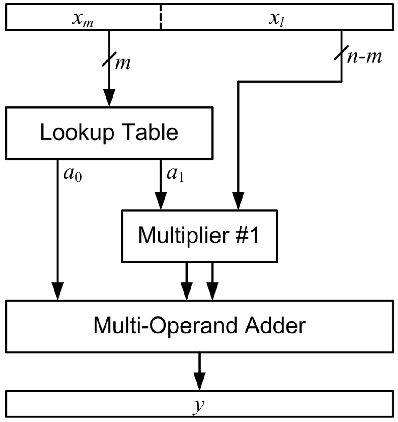In order to reduce the polynomial order while maintaining the desired output accuracy, the interval $[x_{min},x_{max})$ is often partitioned into $2^m$ subintervals of equal size, each with a different set of coefficients. To implement this efficiently in hardware, the interpolator input is split into an m-bit most significant part, $x_m$, and an $(n-m)$-bit least significant part, $x_l$, where n is the number of bits input to the interpolator. For normalized IEEE floating point numbers [31], the input interval for an operand is $[1,2)$. Numbers of this form are specified by the following equation:

$$x=1+x_m+x_l·2^{-m}$$

(2)

The coefficients for each subinterval are stored in a lookup table. $x_m$ is used to select the coefficients, so Equation (1) becomes

$$\begin{array}{ccc}\hfill f\left(x\right)& \approx & a_0\left(x_m\right)+a_1\left(x_m\right)·x+\cdots +a_{N-1}\left(x_m\right)·x^{N-1}\hfill \\ & \approx & \sum _{i=0}^{N-1}{a}_i\left(x_m\right)·x^i\hfill \end{array}$$

(3)

Some applications require function approximation for large operand sizes, such as IEEE double precision formats. Unfortunately, as operand size grows it becomes increasingly difficult to find coefficient sizes and hardware parameters that meet output error specifications with acceptable total hardware complexity. One solution is to relax the precision requirement, e.g., to allow a maximum absolute error of $3/4$ of one unit in the last place (ulp) [32].

Approximation involves the evaluation of a desired function via simpler functions. In this paper, the simpler functions are the polynomials for each interval. Different types of polynomial approximations exist with respect to the error objective, including least-square approximations, which minimize the root-mean-square error, and least-maximum approximations, which minimize the maximum absolute error. For designs with a maximum error constraint, the least-maximum approximations are of interest. The most commonly used least-maximum approximations include the Chebyshev and minimax polynomials. Chebyshev polynomials provide approximations close to the optimal least-maximum approximation and can be constructed analytically. Minimax polynomials provide a better approximation, but must be computed iteratively via the Remez algorithm [33]. Neither Chebyshev nor minimax polynomials account for the combined non-linear effects of coefficient quantization errors, reduction error due to use of truncated arithmetic units and roundoff error due to rounding intermediate values. Our optimization algorithm adjusts the coefficient values to best account for these errors. Chebyshev polynomials are used as the starting point because they are easier to compute and the optimization algorithm only requires reasonable initial coefficient values. Minimax polynomials can also be utilized for the initial approximation, however, this paper focuses on utilizing Chebyshev polynomials.

It is important to consider that the minimax algorithm provides a better approximation utilizing the Remez algorithm compared to the results obtained in this paper, which is discussed later in Section 7. Interestingly, recent research in the area of arithmetic generation has produced minimax approximations automatically using the Remez algorithm [34]. Again, these implementations are complex and designed for Field Programmable Gate Arrays (FPGAs) as denoted on the $FloPoCo$ website [34]. This paper utilizes Chebyshev series approximations, because they provide a simple table-driven method for faithfully-rounded approximation to common elementary functions. Some researchers have also stated that Chebyshev interpolating polynomials are just as good as the best polynomials in the context of table-driven methods for elementary function computations and, thus, the common practice of feeding Chebyshev interpolating polynomials into a Remez procedure offers negligible improvement, if any, and thus may be considered unnecessary [35].

This research targets simple architectures for ASIC implementations. The novel optimization algorithm presented in this paper provides a simple implementation to improve the accuracy of elementary function implementations, especially when using truncated arithmetic units and other approximate arithmetic units [36]. Another advantage is that the methods presented in this paper utilize truncated units that have been shown to exhibit lower power requirements [37]. Other similar endeavors, such as the Sollya project, are useful, but are more complex than the algorithm presented in this paper in addition to having different targets [38]. For example, Sollya is a tool for safe floating-point code development, whereas, the novel direct-search methods in this paper provide another approach that is simple and finds a solution to complex error requirements for elementary functions.

With the approach presented in this paper, Chebyshev series approximations are used to select the initial coefficient values for each subinterval [26,27]. First, the number of subintervals, $2^m$, is determined. With infinite precision arithmetic, the maximum absolute error of a Chebyshev series approximation is [18]

$$\begin{array}{ccc}\hfill & {\displaystyle E_{Chebyshev}=\frac{2^{-N(m+2)+1}·\left|f^n\left(\xi \right)\right|}{N!}}& \\ & x_m\le \xi <x_m+2^{-m}& \hfill \end{array}$$

(4)

where ξ is the point on the interval being approximated such that the Nth derivative of $f\left(x\right)$ is at its maximum value. The maximum allowable error of the interpolator is $2^{-q}$, which is selected as a design parameter. Since there will be error due to finite precision arithmetic in addition to $E_{Chebyshev}$, we limit $E_{Chebyshev}$ to $2^{-q-2}$, and solve Equation (4) for m. Since m must be an integer, this gives

$$m=⌈\frac{q-2N+3+{log}_2\left(\right|f^N\left(\xi \right)\left|\right)-{log}_2(N!)}{N}⌉$$

(5)

The Chebyshev series approximation polynomial, $p_m\left(x\right)$ of degree $N-1$, is computed on the subinterval $[x_m,x_m+2^{-m})$ by the following method:

• The Chebyshev nodes are computed by using

  $${\tau }_i=\cos \left(\frac{(2i+1)·\pi }{2n}\right)\mathrm{for}(0\le \mathrm{i}<\mathrm{n})$$

  (6)
• The Chebyshev nodes are transformed from $[-1,1]$ to $[a,b)$ by the following equation:

  $$x_i=\frac{{\tau }_i(b-a)+(b+a)}{2}\mathrm{for}(0\le \mathrm{i}<\mathrm{n})$$

  (7)

  For subinterval m on $[x_m,x_m+2^{-m})$, this becomes

  $$x_i=x_m+({\tau }_i+1)·2^{-m-1}$$

  (8)
• The Lagrange polynomial, $p_m\left(x\right)$, is formed, which interpolates the Chebyshev nodes on $[x_m,x_m+2^{-m})$ as

  $$p_m\left(x\right)=y_0·L_0\left(x\right)+y_1·L_1\left(x\right)+\cdots +y_{n-1}·L_{n-1}\left(x\right)$$

  (9)

  where $L_i\left(x\right)$ is given in Equation (10)

  $$L_i\left(x\right)=\frac{(x-x_0)·\cdots ·(x-x_{i-1})·(x-x_{i+1})·\cdots ·(x-x_{n-1})}{(x_i-x_0)·\cdots ·(x_i-x_{i-1})·(x_i-x_{i+1})·\cdots ·(x_i-x_{n-1})}$$

  (10)

  and

  $$y_i=f\left(x_i\right)$$

  (11)
• $p_m\left(x\right)$ is expressed in the form given in Equation (9) by combining terms in $p_m\left(x\right)$ that have equal powers of x.
• The coefficients of $p_m\left(x\right)$ are rounded to a specified precision using round-to-nearest even.

2.1. Linear Interpolator Coefficients

For a linear interpolator, the coefficients for the interval $[x_m,x_m+2^{-m})$ are given by

$$\begin{array}{ccc}\hfill a_0& =& -\frac{1}{2}·y_0·\left(\sqrt{2}-1\right)+\frac{1}{2}·y_1·\left(\sqrt{2}+1\right)\hfill \end{array}$$

(12)

$$\begin{array}{ccc}\hfill a_1& =& \sqrt{2}·\left(y_0-y_1\right)·2^{-m}\hfill \end{array}$$

(13)

where

$$\begin{array}{ccc}\hfill y_0& =& f(x_m+2^{-m-1}+\sqrt{2}·2^{-m-2})\hfill \end{array}$$

(14)

$$\begin{array}{ccc}\hfill y_1& =& f(x_m+2^{-m-1}-\sqrt{2}·2^{-m-2})\hfill \end{array}$$

(15)

2.2. Quadratic Interpolator Coefficients

For a quadratic interpolator, the coefficients for the interval $[x_m,x_m+2^{-m})$ are given by

$$\begin{array}{ccc}\hfill a_0& =& \frac{1}{3}·y_0·(2-\sqrt{3})-\frac{1}{3}·y_1+\frac{1}{3}·y_2·(\sqrt{3}+2)\hfill \end{array}$$

(16)

$$\begin{array}{ccc}\hfill a_1& =& \frac{1}{6}·y_0·(\sqrt{3}-4)·2^{m+2}+\frac{1}{3}·y_1·2^{m+4}-\frac{1}{6}·y_2(\sqrt{3}+4)·2^{m+2}\hfill \end{array}$$

(17)

$$\begin{array}{ccc}\hfill a_2& =& \frac{1}{3}·(y_0-2·y_1+y_2)·2^{2m+3}\hfill \end{array}$$

(18)

where

$$\begin{array}{ccc}\hfill y_0& =& f(x_m+(\frac{\sqrt{3}}{2}+1)·2^{-m-1})\hfill \end{array}$$

(19)

$$\begin{array}{ccc}\hfill y_1& =& f(x_m+2^{-m-1})\hfill \end{array}$$

(20)

$$\begin{array}{ccc}\hfill y_2& =& f(x_m+(1-\frac{\sqrt{3}}{2})·2^{-m-1})\hfill \end{array}$$

(21)

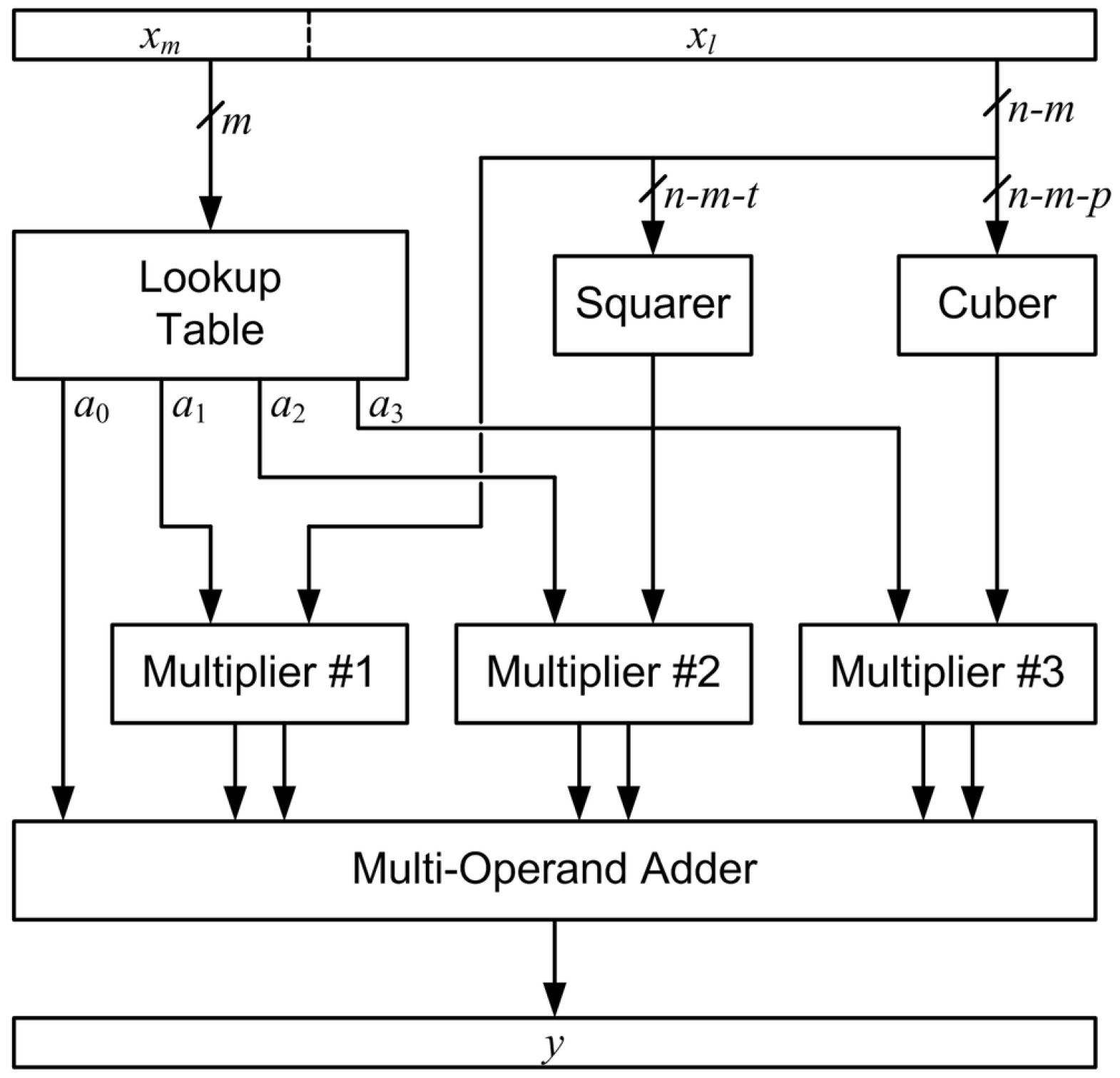
2.3. Cubic Interpolator Coefficients

For a cubic interpolator, the coefficients for the interval $[x_m,x_m+2^{-m})$ are given by Equations (24)–(27) where

$${\kappa }_1=\sqrt{2+\sqrt{2}}$$

(22)

$${\kappa }_2=\sqrt{2-\sqrt{2}}$$

(23)

$$\begin{array}{ccc}\hfill a_0& =& \frac{{\kappa }_2(4{\kappa }_1(y_3+y_0-y_1-y_2)+8y_3-8y_0+{\kappa }_1^3(y_1+y_2))+{\kappa }_1(8y_1-8y_2-{\kappa }_2^3(y_3+y_0))+{\kappa }_1^3(2y_2-2y_1)+{\kappa }_2^3(2y_0-2y_3)}{2{\kappa }_1{\kappa }_2({\kappa }_1-{\kappa }_2)({\kappa }_1+{\kappa }_2)}\hfill \end{array}$$

(24)

$$\begin{array}{ccc}\hfill a_1& =& \frac{2^{m+1}({\kappa }_2(4{\kappa }_1(y_1+y_2-y_3-y_0)+12y_0-12y_3)+\left(12{\kappa }_1(y_2-y_1)\right)+{\kappa }_1^3(y_1-y_2)+{\kappa }_2^3(y_3-y_0))}{{\kappa }_1{\kappa }_2({\kappa }_1-{\kappa }_2)({\kappa }_1+{\kappa }_2)}\hfill \end{array}$$

(25)

$$\begin{array}{ccc}\hfill a_2& =& \frac{2^{2m+3}(({\kappa }_1(y_0-y_1-y_2+y_3)+6{\kappa }_2(y_3-y_0))+6{\kappa }_1(y_1-y_2))}{{\kappa }_1{\kappa }_2({\kappa }_1-{\kappa }_2)({\kappa }_1+{\kappa }_2)}\hfill \end{array}$$

(26)

$$\begin{array}{ccc}\hfill a_3& =& \frac{-2^{3m+5}({\kappa }_2(y_3-y_0)+{\kappa }_1(y_1-y_2))}{{\kappa }_1{\kappa }_2({\kappa }_1-{\kappa }_2)({\kappa }_1+{\kappa }_2)}\hfill \end{array}$$

(27)

$$\begin{array}{ccc}\hfill y_0& =& f\left(x_m+\left(1+\frac{1}{2}\sqrt{2+\sqrt{2}}\right)·2^{-m-1}\right)\hfill \end{array}$$

(28)

$$\begin{array}{ccc}\hfill y_1& =& f\left(x_m+\left(1+\frac{1}{2}\sqrt{2-\sqrt{2}}\right)·2^{-m-1}\right)\hfill \end{array}$$

(29)

$$\begin{array}{ccc}\hfill y_2& =& f\left(x_m+\left(1-\frac{1}{2}\sqrt{2-\sqrt{2}}\right)·2^{-m-1}\right)\hfill \end{array}$$

(30)

$$\begin{array}{ccc}\hfill y_3& =& f\left(x_m+\left(1-\frac{1}{2}\sqrt{2+\sqrt{2}}\right)·2^{-m-1}\right)\hfill \end{array}$$

(31)

One method to reduce the hardware needed to accurately approximate elementary functions using polynomials is to use truncated multipliers and squarers within the hardware [26,27]. Unfortunately, incorporating truncated arithmetic units into the architecture complicates the error analysis. However, recent advances using optimization methods for minimizing the error of a given function using truncated units have been successful at finding an optimal and efficient table size [28]. Furthermore, designs that incorporate truncated multipliers, squarers and cubers significantly reduce area and power consumption required for a given elementary function.

Although many optimization methods can be utilized, the designs generated for this paper utilize a modified form of the cyclic direct search [39]. This optimization method utilizes the optimized most significant bits for each coefficient to significantly reduce the memory requirements. Then, cyclic heuristic direct search is used to optimize the number of truncated columns to decrease the size of the coefficients. Each value is exhaustively tested to ensure that it meets the intended accuracy for a given architecture.

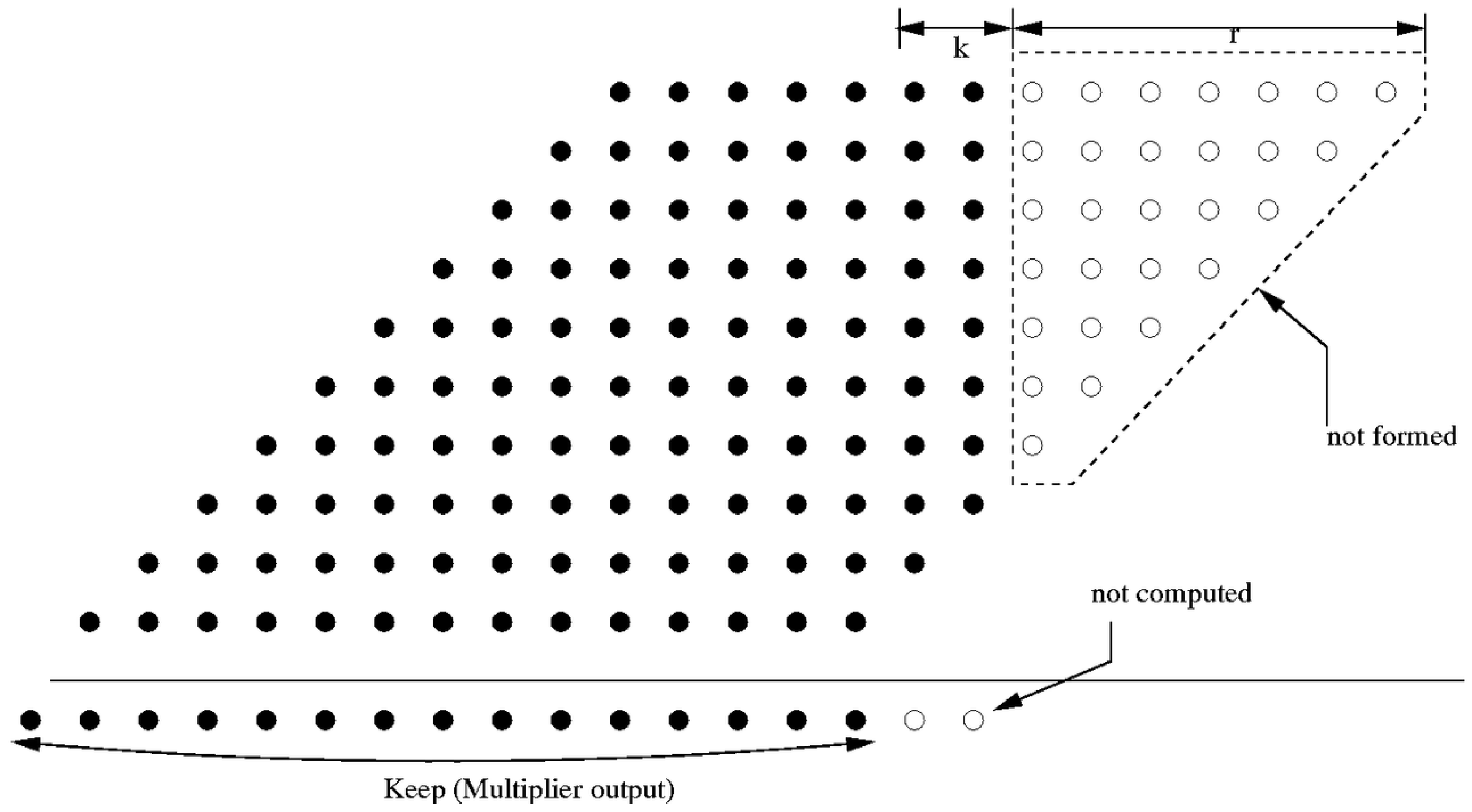
3. Truncated Multipliers, Squarers, and Cubers

Truncated multipliers, squarers, and cubers are units in which several of the least significant columns of partial products are not formed [40]. Eliminating partial products from the multiplication, squaring and cubing matrix reduces the area of the unit by eliminating the logic needed to generate those terms, as well as reducing the number of adder cells required to reduce the matrix prior to the final addition. Additional area savings are realized because a shorter carry-propagate adder can be used to compute the final results, which may yield reduced delay as well. Eliminating adder cells, and thus their related switching activity, also results in reduced power consumption, particularly dynamic power dissipation.

Figure 1 shows a $14\times 10$-bit truncated multiplier, where r denotes the number of unformed columns and k denotes the number of columns that are formed but discarded in the final result. In this example, $r=7$ and $k=2$. Eliminating partial products introduces a reduction error, $E_r$, into the output. This error ranges from $E_{r,low}$, which occurs when each of the unformed partial-product bits is a ‘1’, to $E_{r,high}$, which occurs when each is a ‘0’. $E_{r,low}$ is given by [41]

$$\begin{array}{ccc}\hfill E_{r,low}& =& \sum _{q=0}^{r-1}(q+1)·2^{-2·n+q}\hfill \\ & =& 2^{-r-k-2·n}·((1-r)·2^r+1)\hfill \\ & =& 2^{-r-k}·((1-r)·2^r+1)\mathrm{ulps}\hfill \end{array}$$

(32)

where ulps is units in the last place of the full-width true product. The weight of one ulp depends on the location of the radix point. This analysis assumes that the inputs are between $0\le x<1$. For the example given in Figure 1, $E_{r,high}$ is zero and the range of the reduction error is $-1.502$ ulps $\le E_r\le 0$ ulps. By comparison, the error due to rounding a product using a standard multiplier has a range of $-0.5$ ulps $<E_{rnd}\le 0.5$ ulps (round 0.5 toward $+\infty$ mode).

For truncated squarers, as with truncated multipliers, r denotes the number of unformed columns and k denotes the number of columns that are formed but discarded in the final result. Unlike truncated multipliers, it is not possible for each of the unformed partial-product bits in a truncated squarer to be ‘1’. $E_{r,low}$ for a truncated squarer depends if r is even or odd [42]. If r is even,

$$\begin{array}{ccc}\hfill E_{r,low}& =& -\sum _{q=1}^{r/2-1}((q+1)·2^{2q+1}+(q-1)·2^{2q})-1,\hfill \\ & =& -2^{r-1}·r+2^r-1\hfill \end{array}$$

(33)

If r is odd,

$$\begin{array}{ccc}\hfill E_{r,low}& =& -\sum _{q=1}^{(r-1)/2}(q·(2^{2q}+2^{2q-1}))+2-1+\sum _{q=(r-1)/2}^{r-2}{2}^q+\sum _{q=1}^{(r-1)/2-2}{2}^{2q}\hfill \\ & =& -2^{r-1}·r+11·2^{r-3}-2^{(r/2-1/2)}-1\hfill \end{array}$$

(34)

The reduction error for truncated cubers is [37,43].

$$\begin{array}{ccc}\hfill E_{r,low}& =& \sum _{q=1}^r((q·(q+1))/2)·2^{q-3n}\hfill \end{array}$$

(35)

4. Preliminary Hardware Designs

4.1. Finite Precision Arithmetic Effects

There are several errors that affect the accuracy of the interpolator output. These errors are from the Chebyshev approximation, quantization of coefficients and rounding at the multiplier, squarer and cuber. Quantization error results from rounding each Chebyshev coefficient $a_i$ to $n_i$ bits for storage in a lookup table. Quantization error ϵ is defined as the difference between the infinite precision value and the quantized coefficient. The least significant bit of each coefficient has a weight of $2^{-n_{fi}}$, where $n_{fi}$ is the number of fractional bits in coefficient $a_i$. To prevent large intermediate values, the multiplier, squarer and cuber outputs are rounded. A ‘1’ is added to the column immediately to the right of the rounding point, then the k least significant bits at the output are discarded.

4.2. Linear Interpolator

Figure 2 shows the block diagram of a linear interpolator, where $x_m$ is used to select coefficients $a_0$ and $a_1$ from a lookup table [26,27]. Multiplier #1 computes $a_1·x_l$, which is then added to $a_0$ to produce the output.

Errors in the output due to the quantization of $a_0$ and $a_1$ are $E_{{ϵ}_0}$ and $E_{{ϵ}_1}$ respectively. Since $a_0$ contributes directly to the output, $E_{{ϵ}_0}={ϵ}_0$, and $a_1$ is multiplied by $x_l$ which has a value less than $2^{-m}$, so

$$\begin{array}{ccc}\hfill \left|E_{{ϵ}_0}\right|& \le & 2^{-n_{f0}-1}\hfill \end{array}$$

(36)

$$\begin{array}{ccc}\hfill \left|E_{{ϵ}_1}\right|& \le & 2^{-n_{f1}-1}·2^{-m}\hfill \end{array}$$

(37)

The design goal is to limit the absolute error of the interpolator output to $2^{-q}$, where q is selected based on the overall accuracy requirements. Each coefficient length is chosen by setting $E_{{ϵ}_i}=2^{-q-3}$ and solving for $n_{fi}$. This ensures that $E_{{ϵ}_0}+E_{{ϵ}_1}\le 2^{-q-2}$. In addition to the fractional bits, a sign bit is needed, so

$$\begin{array}{ccc}\hfill n_0& =n_{f0}+1& =q+3\hfill \end{array}$$

(38)

$$\begin{array}{ccc}\hfill n_1& =n_{f1}+1& =q-m+3\hfill \end{array}$$

(39)

In addition to quantization errors, rounding the multiplier output introduces a rounding error $E_{rnd\_m1}$ at the interpolator output. The LSB (least significant bit) weight of $a_1$ is $2^{-n_{f1}}$ and the LSB weight of $x_l$ is $2^{-n}$, so the LSB weight of a full precision product would be $2^{-n_{f1}-n}$. Since r columns of partial products are not formed and k output bits are discarded, the LSB weight of the multiplier output is $2^{-n_{f1}-n+k_{m1}+r_{m1}}$, so $E_{rnd\_m1}\le 2^{-n_{f1}-n+k_{m1}+r_{m1}-1}$, where $k_{m1}$ and $r_{m1}$ are k and r for the multiplier.

The design is initiated by first using standard multipliers. We want the rounding error to be less than the error due to coefficient quantization, so $k_{m1}$ is chosen by setting $E_{rnd\_m1}=2^{-q-4}$ and solving for $k_{m1}$. Remember that for a standard multiplier, all columns of partial products are formed, so $r=0$ and

$$k_{m1}=n-m-1$$

(40)

4.3. Quadratic Interpolator

Figure 3 shows the block diagram of a quadratic interpolator, where $x_m$ is used to select coefficients $a_0$, $a_1$ and $a_2$ from a lookup table [26,27]. A specialized squarer computes $x_l^2$. Multiplier #1 computes $a_1·x_l$ and multiplier #2 computes $a_2·x_l^2$, which are then added to $a_0$ to produce the output.

As with the linear interpolator, the multiplier outputs can be kept in carry-save form. $E_{{ϵ}_0}$ and $E_{{ϵ}_1}$ for a quadratic interpolator are the same as for a linear interpolator, given by Equations (36) and (37). $a_2$ is multiplied by the squarer output, which has a maximum value of $2^{-2m}$, so

$$\left|E_{{ϵ}_2}\right|\le 2^{-n_{f2}-1}·2^{-2m}$$

(41)

As with the linear interpolator, the design goal is to limit the approximation error to $2^{-q}$. In the case of the quadratic interpolator, however, there are three errors due to coefficient quantization as well as several rounding errors, so we initially set each $E_{{ϵ}_i}$ equal to $2^{-q-4}$ rather than $2^{-q-3}$ to ensure that the sum of all errors is less than $2^{-q}$. A sign bit is required in addition to the fractional bits so

$$\begin{array}{ccc}\hfill n_0& =n_{f0}+1& =q+4\hfill \end{array}$$

(42)

$$\begin{array}{ccc}\hfill n_1& =n_{f1}+1& =q-m+4\hfill \end{array}$$

(43)

$$\begin{array}{ccc}\hfill n_2& =n_{f2}+1& =q-2m+4\hfill \end{array}$$

(44)

Analysis shows that for some configurations, $x_l$ can be truncated at the input to the squarer to reduce the size of the squarer. Assume that the t least significant bits of $x_l$ are truncated, such that $x_l=x_l^{\prime }+{ϵ}_{x_l}$, where $x_l^{\prime }$ is the truncated version of $x_l$. The squarer output is then ${x_l^{\prime }}^2$ rather than $x_l^2$, resulting in a squarer output error of $-2x_l^{\prime }·{\epsilon }_{x_l}-{\epsilon }_{x_l}^2$. Noting that $x_l^{\prime }<2^{-m}$, $|{\epsilon }_{x_l}|<2^{-n+t}$, and ${\epsilon }_{x_l}^2$ is negligible, the magnitude of the squarer output error is less than $2^{-n-m+t+1}$. This error is then multiplied by $a_2$, so the error at the interpolator output due to ${ϵ}_{xl}$ is

$$\left|E_{{ϵ}_{x_l}}\right|\le 2^{-n-m+t+1}$$

(45)

assuming $\left|a_2\right|\le 1$. The value of $E_{{\epsilon }_{x_l}}$ is set equal to $2^{-q-4}$ to find the maximum value for t, which gives

$$t=n+m-q-5$$

(46)

If $t\le 0$, then $x_l$ cannot be truncated. As with the linear interpolator, we set k for the multipliers and the squarer so that rounding error in each unit is less than each error due to quantization. Since we limited each quantization error to $2^{-q-4}$, we limit each rounding error to $2^{-q-5}$.

Like the linear interpolator, the LSB weight of the multiplier #1 output is $2^{-n_{f1}-n+k_{m1}+r_{m1}}$, resulting in $E_{rnd\_m1}=2^{-n_{f1}-n+k_{m1}+r_{m1}-1}$. Setting this equal to $2^{-q-5}$ gives

$$k_{m1}=n-m-1$$

(47)

The LSB weight of the squarer output is $2^{-2n+2t+k_{sq}+r_{sq}}$, so $E_{rnd\_sq}=2^{-2n+2t+k_{sq}+r_{sq}-1}$, where $k_{sq}$ and $r_{sq}$ are k and r for the squarer. The squarer output is multiplied by $a_2$, where we assume $|a_2|\le 1$, so the rounding error for the squarer is set equal to $2^{-q-4}$ to find $k_{sq}$

$$k_{sq}=2n-2t-q-3$$

(48)

If $\left|a_2\right|>1$, $k_{sq}$ is increased accordingly.

The LSB weight of the multiplier #2 output is $2^{-n_{f2}-2n+2t+k_{sq}+r_{sq}+k_{m2}+r_{m2}}$ so $E_{rnd\_m_2}=2^{-n_{f2}-2n+2t+k_{sq}+r_{sq}+k_{m2}+r_{m2}-1}$. Setting the maximum rounding error equal to $2^{-q-5}$ gives

$$k_{m2}=q-2m+3$$

(49)

4.4. Cubic Interpolator

Figure 4 shows the block diagram of a cubic interpolator. The m most significant bits of x, $x_m$, are used to select coefficients $a_0$, $a_1$, $a_2$ and $a_3$ from a lookup table. A specialized squarer computes $x_l^2$ and a specialized cuber computes $x_l^3$. Multiplier #1 computes $a_1·x_l$, multiplier #2 computes $a_2·x_l^2$ and multiplier #3 computes $a_3·x_l^3$, all of which are then added to $a_0$ to produce the output. All of the multiplier outputs are kept in carry-save form.

Errors in the output due to the quantization of $a_0$, $a_1$, $a_2$ and $a_3$ are $E_{{\epsilon }_0}$, $E_{{\epsilon }_1}$, $E_{{\epsilon }_2}$ and $E_{{\epsilon }_3}$ respectively. Since $a_0$ contributes directly to the output, $E_{{\epsilon }_0}={\epsilon }_0$, so

$$|E_{{\epsilon }_0}|\le 2^{-n_{f0}-1}$$

(50)

Coefficient $a_1$ is multiplied by $x_l$, which has a maximum value less than $2^{-m}$, so

$$|E_{{\epsilon }_1}|<2^{-n_{f1}-1}·2^{-m}$$

(51)

Coefficient $a_2$ is multiplied by the squarer output, which has a maximum value of $2^{-2m}$, so

$$|E_{{\epsilon }_2}|<2^{-n_{f2}-1}·2^{-2m}$$

(52)

Coefficient $a_3$ is multiplied by the cuber output, which has a maximum value of $2^{-3m}$, so

$$|E_{{\epsilon }_3}|<2^{-n_{f3}-1}·2^{-3m}$$

(53)

The design goal is to limit the approximation error to $2^{-q}$. In the case of the cubic interpolator there are four errors due to coefficient quantization as well as several rounding errors, so we initially set each $E_{{\epsilon }_i}$ equal to $2^{-q-5}$ to ensure that $\sum E_{{\epsilon }_i}<2^{-q-3}$, and the sum of all errors is less than $2^{-q}$. Utilizing a sign bit in addition to the fractional bits, the sizes of the coefficients are as follows:

$$\begin{array}{ccc}\hfill n_0& =n_{f0}+1& =q+5\hfill \end{array}$$

(54)

$$\begin{array}{ccc}\hfill n_1& =n_{f1}+1& =q-m+5\hfill \end{array}$$

(55)

$$\begin{array}{ccc}\hfill n_2& =n_{f2}+1& =q-2m+5\hfill \end{array}$$

(56)

$$\begin{array}{ccc}\hfill n_3& =n_{f3}+1& =q-3m+5\hfill \end{array}$$

(57)

Like the linear and quadratic interpolators, the LSB weight of the multiplier #1 output is $2^{-n_{f1}-n+k_{m1}+r_{m1}}$, resulting in $E_{rnd\_m1}=2^{-n_{f1}-n+k_{m1}+r_{m1}-1}$. The rounding error is chosen to be less than the error due to coefficient quantization, so $E_{rnd\_m1}$ is set equal to $2^{-q-6}$ which gives

$$k_{m1}=n-m-1$$

(58)

Similar to the quadratic interpolator, $x_l$ can be truncated at the input to the squarer. The error at the interpolator output due to the truncation of $x_l$ is set equal to $2^{-q-5}$ to find the maximum value of t, which gives

$$t=n+m-q-6$$

(59)

The rounding error for the squarer is set equal to $2^{-q-6}$ to find $k_{sq}$, which gives

$$k_{sq}=2n-2t-q-5$$

(60)

The maximum rounding error for multiplier #2 is set to $2^{-q-6}$, which gives

$$k_{m2}=q-2m+1$$

(61)

Again, similar to the squarer, the input to the cuber can be truncated. Assume that the p least significant bits of $x_l$ are truncated, such that $x_l=x_l^{\prime \prime }+{\epsilon }_{x_l}$, where $x_l^{\prime \prime }$ is the truncated version of $x_l$ that is input to the cuber. The cuber output is then ${x_l^{\prime \prime }}^3$ rather than $x_l^3$, resulting in a cubic output error of $-3{x_l^{\prime \prime }}^2·{\epsilon }_{x_l}-3x_l^{\prime \prime }·{\epsilon }_{x_l}^2-{\epsilon }_{x_l}^3$. Noting that ${x_l^{\prime \prime }}^2<2^{-2m}$, $|{\epsilon }_{x_l}|<2^{-n+p}$ and that ${\epsilon }_{x_l}^2$ and ${\epsilon }_{x_l}^3$ are negligible, the magnitude of the cuber output error is less than $3·2^{-n-2m+p}$. This error is then multiplied by $a_3$, so the error at the interpolator output due to ${\epsilon }_{x_l}$ is

$$|E_{{\epsilon }_{x_l}}|<2^{-n-2m+p+1}$$

(62)

assuming $|a_3|\le 1$. As done previously, the value of $E_{{\epsilon }_{x_l}}$ is set equal to $2^{-q-5}$ to find the maximum value for p, which gives

$$p=n+2m-q-6$$

(63)

The LSB weight of the cuber output is $2^{-3n+3p+k_{cu}-r_{cu}}$, so $E_{rnd\_cu}=2^{-3n+3p+k_{cu}-r_{cu}-1}$, where $k_{cu}$ and $r_{cu}$ are k and r for the cuber. The cuber output is multiplied by $a_3$, where it is assumed that $|a_3|\le 1$, so the rounding error for the cuber is set equal to $2^{-q-6}$ to find $k_{cu}$ which gives

$$k_{cu}=3n-3p-q-5$$

(64)

If $|a_3|>1$, then $k_{cu}$ is increased accordingly.

The LSB weight of the multiplier #3 output has a value of $2^{-n_{f3}-3n+3p+k_{cu}+r_{cu}+k_{m3}+r_{m3}}$, so the rounding error is $E_{rnd\_m3}=2^{-n_{f3}-3n+3p+k_{cu}+r_{cu}+k_{m3}+r_{m3}-1}$. Setting the maximum rounding error equal to $2^{-q-6}$ gives

$$k_{m3}=q-3m+5$$

(65)

Although there are several ways to add all the partial products to produce the output, y, each method benefits from having fewer partial products. In this paper, Dadda reduction schemes are used for the multipliers in each design [44]. The constant correction method [41] is used for all truncated multipliers, squarers and cubers. Although other correction methods can be employed, constant correction is the easiest to implement. However, any correction scheme could be used.

5. Coefficient Optimization

After the preliminary design is completed, the coefficients are adjusted based on precision. To minimize the lookup table size based on the term m, the direct search method is selected to find the minimum MSB (most significant bit) of each interpolator. The size of the lookup table is $2^m·(n_0+n_1)$ for a linear interpolator, $2^m·(n_0+n_1+n_2)$ for a quadratic interpolator, and $2^m·(n_0+n_1+n_2+n_3)$ for a cubic interpolator. Finding the minimum value of m where the output precision requirement can be met for all of the values in the reduced input domain reduces the size of the lookup table.

Initially, standard multipliers (full-width, all columns formed) are used. After the optimized value of m is computed, each coefficient is found. Next, the standard multipliers, squarer and cuber are replaced with truncated units. A new optimization method called the cyclic heuristic direct search is used to maximize the number of unformed columns while maintaining design specifications for error. This optimization reduces the area of the computational portion of the interpolator at the same time coefficient sizes are optimized, reducing the size of the lookup table. For example, consider the multiplier that computes $a_1·x_l$ in a linear interpolator and note that reducing the size of $a_1$ also reduces the size of the partial-product matrix required. Quadratic interpolators have two terms to optimize, $a_1$ and $a_2$, and cubic interpolators have three terms to optimize, $a_1$, $a_2$ and $a_3$. Cyclic heuristic direct search is used because it is well suited for discrete optimization in multivariable equations.

Discrete optimization means searching for an optimal solution in a finite or countably infinite set of potential solutions. Optimality is defined with respect to some criterion function, which is to be minimized or maximized. In the cyclic heuristic direct search method each iteration involves a “cyclic” cycle in which each dependent variable makes an incremental change in value, one at a time, then repeats the cycle [39].

5.1. Optimization Method

In the first stage, the number of most-significant bits, m, of the value input to the interpolator, x, is optimized such that the function, $y\left(x\right)$, is approximated to the specified accuracy. The decision variable, DV, is $\mathrm{DV}=m$ and the objective function, OF, is $\mathrm{OF}=m$. The constraint is $\left|y{\left(x\right)}_{Real}-y{\left(x\right)}_{Approx}\right|\le 2^{-q}$ for all $x\in [1,2)$, where $y{\left(x\right)}_{Real}$ is the exact value of the function, $y{\left(x\right)}_{Approx}$ is the approximated value of the function and q is the number of bits of precision in the output. The algorithm adjusts the DV to minimize the OF. Direct search methods are known as unconstrained optimization techniques that do not employ a derivative (gradient) [39].

In the second stage, the coefficients sizes are optimized (minimized) and the number of unformed columns in the arithmetic units are optimized (maximized) at the same time. This further reduces the required size of the lookup tables and reduces the sizes of the partial-product matrices, which reduces the overall area, delay and power of the interpolator.

For the second stage, the cyclic heuristic direct search method is used for several reasons. The algorithm is simple to understand and implement. Direct searches can also satisfy hard constraints well and do not use a derivative, gradient or Hessian, which have difficulty coping with non-analytic surfaces such as ridges, discontinuities in the function or slope, and add computational difficulty and programming complexity. Simplicity, robustness, and accommodation of constraints in this algorithm are significant advantages for use with elementary function error analysis. Each of the coefficients values are adjusted to satisfy the accuracy requirements.

Linear interpolators have 2 DVs, the size of coefficients for $a_0$ and $a_1$. The objective function is

$$\mathrm{OF}=-r_{m1}$$

(66)

As with the first stage, the algorithm adjusts the DVs to minimize the OF. This paper addresses maximizing the number of unformed columns. Therefore, Equation (66) is chosen because minimizing OF will maximize $r_{m1}$. Other optimization algorithms may adjust the DVs to maximize the OF [39]. If our algorithm maximized the OF then $\mathrm{OF}=r_{m1}$ would be used.

Quadratic interpolators have 3 DVs, the size of coefficients $a_0$, $a_1$, and $a_2$. The objective function is

$$\mathrm{OF}=-(r_{m_1}+r_{m_2}+r_{sq})$$

(67)

Finally, cubic interpolator designs have 4 DVs, the size of coefficients $a_0$, $a_1$, $a_2$, and $a_3$. The objective function is

$$\mathrm{OF}=-(r_{m_1}+r_{m_2}+r_{m_3}+r_{sq}+r_{cu})$$

(68)

The constraint is ${|y\left(x\right)}_{Real}-y{\left(x\right)}_{Approx}|<2^{-q}$ for faithful rounding, but can be modified for different precision requirements.

The procedure for the cyclic heuristic direct search method is:

• Initialize the Decision Variable base (the initial trial solution in a feasible region), ${\mathrm{DV}}_{\mathrm{base}}$, and evaluate the Objective Function, OF.
• Start the cycle for one iteration.
• Taking each DV, one at a time, set the new trial DV value,

  $${\mathrm{DV}}_{\mathrm{trial}}={\mathrm{DV}}_{\mathrm{base}}+\Delta \mathrm{DV}$$

  (69)
• Evaluate the function at the trial value. If worse or “FAIL” keep DV base and set $\Delta {\mathrm{DV}}_{\mathrm{i}}$ to a smaller change in the opposite direction, where contract and expand are names arbitrarily chosen as constants used for adjustment in the optimization, such that contract is $-1$ and expand is $+1$.

  $$\Delta {\mathrm{DV}}_i=\mathrm{contract}·\Delta {\mathrm{DV}}_i$$

  (70)
• Otherwise, keep the better solution (make it the base point) and accelerate moves in the correct direction

  $$\begin{array}{ccc}\hfill {\mathrm{OF}}_{\mathrm{base}}& =& {\mathrm{OF}}_{\mathrm{trial}}\hfill \end{array}$$

  (71)

  $$\begin{array}{ccc}\hfill {\mathrm{DV}}_{\mathrm{base}}& =& {\mathrm{DV}}_{\mathrm{trial}}\hfill \end{array}$$

  (72)

  $$\begin{array}{ccc}\hfill \Delta {\mathrm{DV}}_i& =& \mathrm{expand}·\Delta {\mathrm{DV}}_i\hfill \end{array}$$

  (73)
• At the end of the cycle check for stopping criteria (excessive iterations, or convergence criteria met).
• Stop, or repeat from Step 2.

5.2. Optimization Example and Results

This Section presents a function approximation example to help clarify how the optimization method works and how it improves results. Real numbers equal to the underlying fixed-point binary values, then rounded to 6 fractional digits, are given in the example to improve readability. For the sake of example, an arbitrary chosen input value for the interpolator, $x=1.278498$, which has a reciprocal value $y\left(x\right)=0.782168$. The cyclic heuristic direct search method is employed to find the coefficient values used to compute the approximation of the reciprocal in a similar fashion as the interpolators in this paper.

Table 1. Example approximation calculation, $x=1.278498$, $y\left(x\right)=1/x$.

Interpolator	n	m	${\mathit{x}}_{\mathit{m}}$	${\mathit{x}}_{\mathbf{l}}$	${\mathit{y}}_{\mathbf{0}}$	${\mathit{y}}_{\mathbf{1}}$	${\mathit{y}}_{\mathbf{2}}$	${\mathit{y}}_{\mathbf{3}}$	${\mathit{a}}_{\mathbf{0}}$	${\mathit{a}}_{\mathbf{1}}$	${\mathit{a}}_{\mathbf{2}}$	${\mathit{a}}_{\mathbf{3}}$	$\mathit{y}{\left(\mathit{x}\right)}_{\mathit{Approx}}$
Linear	16	7	1.265625	0.012873	0.785982	0.789410	-	-	0.785171	−0.612738	-	-	0.782180
Quadratic	16	4	1.250000	0.028498	0.764342	0.780488	0.797329	-	0.799997	−0.639162	0.475655	-	0.782169
Cubic	16	3	1.250000	0.028498	0.729798	0.748269	0.776046	0.796966	0.799999	−0.639868	0.506617	−0.337745	0.782163
Linear	24	11	1.278320	0.000177	0.782022	0.782233	-	-	0.782277	−0.611723	-	-	0.782168
Quadratic	24	7	1.265625	0.012873	0.783035	0.784074	0.785115	-	0.785276	−0.616655	0.482027	-	0.782168
Cubic	24	5	1.250000	0.028498	0.781213	0.786408	0.793874	0.799240	0.799999	−0.639998	0.511617	−0.389804	0.782168
Cubic	32	7	1.265625	0.012873	0.782965	0.783614	0.784533	0.785184	0.785276	−0.616659	0.484242	−0.377945	0.782168

shows the value of the approximation using linear, quadratic and cubic methods described in the paper. The n-bit range-reduced input to the interpolator, x, is partitioned into $2^m$ sub-intervals, each with its own set of coefficients $a_0$ through $a_{N-1}$. $x_m$ is the m most significant bits of x and $x_l$ is the $n-m$ least significant bits of x. Although any analytical function can be shown using the results in this paper, reciprocal is utilized as an example as it is one of the more common implementations.

For a linear interpolator, the initial values of the coefficients $a_0$ and $a_1$ are found for each sub-interval using Equations (12) and (13), where $y_0$ and $y_1$ are given by Equations (14) and (15). The coefficients are then optimized and the number of unformed columns in the truncated arithmetic units are found using the method described in Section 5.

Table 2. Coefficient sizes for regular multipliers vs. optimized truncated multipliers, squarers and cubers, $f\left(x\right)=1/x$.

Interpolator	n	${\mathit{n}}_{\mathbf{0}}$		${\mathit{n}}_{\mathbf{1}}$		${\mathit{n}}_{\mathbf{2}}$		${\mathit{n}}_{\mathbf{3}}$
		Regular	Optimized	Regular	Optimized	Regular	Optimized	Regular	Optimized
Linear	16	18	18	11	8	-	-	-	-
Quadratic	16	19	19	15	11	11	11	-	-
Cubic	16	20	20	17	12	14	12	11	10
Linear	24	26	26	15	12	-	-	-	-
Quadratic	24	27	27	20	14	13	13	-	-
Cubic	24	28	28	23	14	18	14	13	12
Cubic	32	36	36	29	16	22	16	15	14

shows the coefficients sizes for each interpolator utilizing traditional multiplication and no optimization compared to using the cyclic heuristic direct search optimization method with truncated multipliers, squarers and cubers. For example, with the 32-bit cubic interpolator the initial size of $a_1$ is 29 bits, which is then reduced to 16 bits after optimization. This significant reduction in size not only reduces the size of the lookup table, it also significantly reduces the size of the multiplier that computes $a_1·x_l$, which further reduces area, delay and power in the interpolator. Previous methods of computing the error for each memory or hardware unit relied on trial and error, while the method provided in this paper utilizes an optimal way of finding the coefficients for each table as well as containing the error within all multipliers.

Table 3. Arithmetic units required for faithfully rounded results, $f\left(x\right)=1/x$.

Interpolator	n	Multiplier $\mathbf{\#}\mathbf{1}$			Multiplier $\mathbf{\#}\mathbf{2}$			Multiplier $\mathbf{\#}\mathbf{3}$		Squarer			Cuber		Adder Widths
		Ours	[18]	[26]	Ours	[18]	[26]	Ours	[18]	Ours	[18]	[26]	Ours	[18]	Ours	[18]	[26]
Linear	16	$8\times 9$	$15\times 5$	$9\times 9$	-	-	-	-	-	-	-	-	-	-	18,10	24,16	18, 11
Quadratic	16	$11\times 12$	$19\times 8$	$15\times 12$	$11\times 12$	$12\times 10$	$12\times 12$	-	-	11	12	11	-	-	19,13,13	24,21,14	19,16,13
Cubic	16	$12\times 13$	$22\times 10$	-	$12\times 16$	$17\times 16$	-	$10\times 16$	$12\times 12$	13	16	-	13	12	20,16,16,16	25,23,18,13	-
Linear	24	$12\times 13$	$21\times 6$	-	-	-	-	-	-	-	-	-	-	-	26,24	36,22	-
Quadratic	24	$14\times 17$	$31\times 12$	$20\times 17$	$13\times 17$	$19\times 16$	$13\times 14$	-	-	15	17	15	-	-	27,18,17	40,33,21	26,21,14
Cubic	24	$14\times 19$	$35\times 15$	-	$14\times 24$	$27\times 24$	-	$12\times 24$	$18\times 14$	19	24	-	19	14	28,24,24,24	41,37,29,20	-
Cubic	32	$16\times 25$	-	-	$16\times 32$	-	-	$14\times 32$	-	25	-	-	25	-	36,32,32,32	-	-

shows the hardware requirements comparison between our results and previous research methods.

Table 4. Memory requirements for faithfully rounded results, $f\left(x\right)=1/x$.

		Coefficient Lengths
Interpolator	n	${\mathit{a}}_{\mathbf{0}}$			${\mathit{a}}_{\mathbf{1}}$			${\mathit{a}}_{\mathbf{2}}$			${\mathit{a}}_{\mathbf{3}}$		Lookup Table Size
		Ours	[18]	[26]	Ours	[18]	[26]	Ours	[18]	[26]	Ours	[18]	Ours	[18]	[26]
Linear	16	18	24	18	8	15	11	-	-	-	-	-	2944	156,000	3072
Quadratic	16	19	24	19	11	19	15	11	12	12	-	-	592	27,500	672
Cubic	16	20	25	-	12	22	-	12	17	-	10	12	360	9500	-
Linear	24	26	36	-	12	21	-	-	-	-	-	-	73,728	28,500,000	-
Quadratic	24	27	40	26	14	31	20	13	19	13	-	-	6272	1,440,000	7040
Cubic	24	28	41	-	14	35	-	14	27	-	12	18	2100	121,000	-
Cubic	32	36	-	-	16	-	-	16	-	-	14	-	11,300	-	-

shows the memory requirements comparison between our results with [18,26].

Table 5. Optimized bit-widths and lookup table sizes for various functions.

Function	Linear 16		Linear 24		Quadratic 16		Quadratic 24		Cubic 16		Cubic 24		Cubic 32
	m	Table Size	m	Table Size	m	Table Size	m	Table Size	m	Table Size	m	Table Size	m	Table Size
$1/x$	7	2944	11	73,728	4	592	7	6272	3	360	5	2100	7	11,300
$\sqrt{x}$	6	1664	9	19,968	4	576	6	3456	3	368	4	1152
$1/\sqrt{x}$	7	3072	10	37,888	4	560	7	6400	3	360	5	2112
$sin\left(x\right)$	6	1152	10	39,939	5	1088	7	6656	3	360	5	2080

shows the results for determining the optimal bit-width of the coefficients and their respective lookup table sizes for four elementary functions: reciprocal, square root, reciprocal square root and sine. All values were computed in MATLAB using a script run on a 2.28 GHz Apple MacPro QuadCore Intel Xeon with 4 GB of 800 MHz DDR2 memory. Run times, even for 32-bit cubic interpolators, are under 1 minute for all cases.

The importance of the results is that they seek to find a near-optimal solution of the lowest memory requirements for a given elementary function. The exploration space is based on the input operand space (e.g., 32 bits). Consequently, an exhaustive search for finding the smallest optimal decomposition for a given operand size could take a considerable amount of time. The difficulty in finding these table sub-divisions (e.g., $a_0$ and $a_1$ in Figure 2) is that each configuration has to run over the total space of the register size. That is, a specific 32-bit operand decomposition would have to exhaustively check all $2^{32}$ configurations to find the worst-case error and see if the stopping criterion of being faithfully rounded is met. As a comparison, traditional exhaustive searches (i.e., checking each configuration for a given operand size one by one) ran several weeks with no tangible result. On the other hand, the algorithms and presented architectures discussed in this research are realizable and complete within a reasonable amount of time for the appropriate sizes presented. Future research might explore looking at larger operand sizes, such as 64 and 128 bits, for more accurate and reliable computations.

6. Implementation Results

The approach described in Section 5 is implemented using a MATLAB script. The script computes the optimized polynomial coefficients and the maximum number of columns that can be removed from the truncated arithmetic units. Synthesizable Verilog descriptions are then created for linear, quadratic and cubic architectures. Code written in C is used to generate optimized RTL-level Verilog descriptions of the squaring and cubing units used in the interpolators. The Verilog descriptions have been implemented, targeting a 65nm cmos10lpe bulk CMOS technology from IBM^®. Results are obtained using Synopsys^® (formerly Virage Logic) standard-cell libraries and synchronous-based memory compilers. Memories are generated from the compiler to best suit their intended implementation size. Interestingly, most memories do not fit the exact required memory size, so they have empty space that may affect the area and delay estimates. Because of this, the results might be significantly better if the memory compiler could produce sizes that fit the required interpolator size more accurately, such as with some open-source memory compilers [45]. Designs were synthesized using Synopsys^® Design Compiler™ and the layout was produced using Synopsys^® IC Compiler (ICC)™. Power numbers are generated from parasitic extraction of the layout and $100,000$ random input vectors using Synopsys^® PrimeTime™.

Both compiler-generated memories and standard-cells are placed and routed together to form the best aspect ratio and area for the smallest delay. The methods employed in this paper are optimized for delay, because the interpolators dominate the total area cost, which is especially true as the operand size increases. Although smaller operand sizes could be produced with random logic, the intended applications for this paper typically use memory-driven layouts (e.g., within multiplicative-division schemes inside general-purpose architecture datapaths). Therefore, to create a consistent comparison all implementations utilize memory generated by a memory compiler.

This paper produces several designs by varying the precision, the architecture, and the approximation order. For this paper, several word sizes are designed for the linear, quadratic and cubic architectures using the function $f\left(x\right)=1/x$ for $x\in [1,2)$. The area and delay results for 16, 24 and 32-bit interpolators are reported in

Table 6. Post-layout area and delay results, $f\left(x\right)=1/x$.

Interpolator	n	No. Mem	Memory Sizes	No. Cells	Area (${\mathbf{mm}}^{\mathbf{2}}$)	Memory Delay (ns)	Total Delay (ns)
			$512\times 18$
Linear	16	2	$512\times 10$	734	0.0416	1.128	1.895
			$512\times 20$
Quadratic	16	3	$512\times 14$	2494	0.0783	1.147	2.319
			$512\times 10$
			$512\times 20$
			$512\times 12$
Cubic	16	4	$512\times 12$	5011	0.0957	1.220	2.780
			$512\times 10$
			$2048\times 26$
Linear	24	2	$2048\times 14$	1522	0.1019	1.300	2.217
			$512\times 28$
Quadratic	24	3	$512\times 18$	4729	0.1120	1.160	2.330
			$512\times 12$
			$512\times 28$
			$512\times 14$
Cubic	24	4	$512\times 14$	9945	0.1292	1.170	3.150
			$512\times 12$
			$512\times 36$
			$512\times 16$
Cubic	32	4	$512\times 16$	15,351	0.3956	1.260	3.410
			$512\times 14$

. It can be seen that the piecewise-linear implementation has a unit in the last position (ulp) of $2^{-16}$ that is more efficient than the quadratic interpolator circuit. For 16-bit accuracy, the linear interpolator has smaller area requirements yet maintains high speed with smaller utilization of standard cells compared to quadratic and cubic interpolators. On the other hand, the 24-bit quadratic interpolator is more efficient than the linear interpolator yet requires approximately $3.5$ times more area. For 16-bit accuracy, the area requirements are smaller, yet it still maintains its high speed with smaller utilization of standard cells compared to 24 bits. For cubic implementation, the 24-bit cubic interpolator is more efficient than the 16-bit interpolator despite having around $35\%$ more area than 16-bit architectures. On the other hand, 32-bit architectures have significantly more area than 16 and 24 bits, yet have comparable speed.

For all of the results in Table 6, the total delay is the post-layout critical path through the circuit including the memory delay. The memory delay is highlighted in Table 6 to showcase the non-memory delay (i.e., Non-memory Delay = Total Delay - Memory Delay). Since the memory is synchronous, the memory is read on the clock half-cycle and processed on the subsequent clock half cycle. Therefore, an asynchronous memory design may improve the critical path, since it does not have to wait for the precharge tied to the clock. It is important to also consider that the implementations utilized in this paper use actual extracted memory instantiations as opposed to logic produced from FPGAs. Previous research [14] has utilized specific FPGAs that have embedded memories, such as Xilinx’s Block RAM (BRAM). Implementations using BRAM usually have integrated columns arranged throughout the FPGA and allocate single columns of memory at a time when needed. When a specific FPGA implementation gets large, it has to route its implementation across multiple columns and, thus, possibly skew the actual propagation times because the place and route of the slices are not efficiently located [46]. Although previous research could theoretically implement architectures that could use their columns efficiently, it is hard to tell for a given implementation unless otherwise specified.

Some alternative architectures have been proposed to help alleviate some of these problems, such as Xilinx’s UltraScale Architecture [47]. However, the gap between implementations of silicon and FPGAs can be considerable based on the actual floorplan of its implementation and its routing. Therefore, this paper focuses on implementations utilizing dedicated low-power SRAM implementations and standard-cell logic that have optimized floorplans. An argument could also be made that a full-custom design (for both memory and logic) would produce better results, as well. On the other hand, the implementations in this paper are as close to a full-custom implementation as possible in terms of their implementation. Also, similar to the research presented in [20], there is a tradeoff between the size of the memory and the amount of logic for these dedicated interpolators, as shown in Table 6.

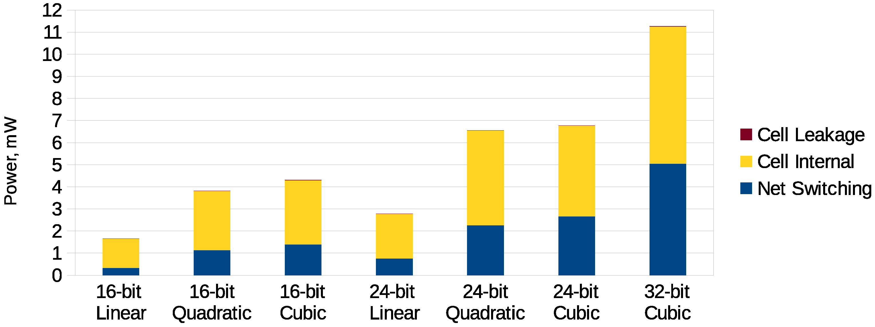
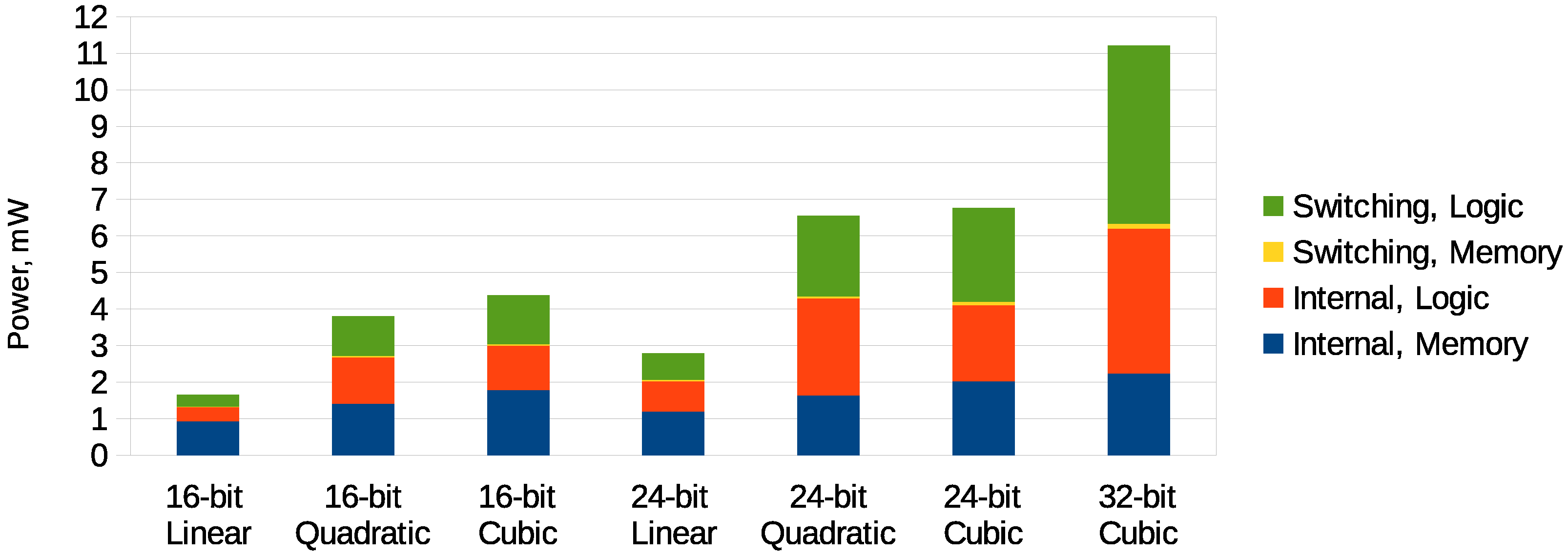
The power results for linear, quadratic and cubic with 16, 24 and 32-bit precisions are reported in Figure 5 and Figure 6. Figure 5 shows the dynamic and leakage power for each interpolator based on generating several thousand random input vectors. It can be seen that increasing the complexity of hardware increases the power dissipation. Figure 6 shows the dynamic power and percentage of memory and logic circuit power usage separately. Interestingly, both quadratic methods incurred a small amount of power for their clock networks (not shown due to the small amount reported), whereas, linear methods do not.

7. Memory Comparison

A comparison of the optimized Chebyshev quadratic and cubic interpolators with existing methods for function approximation is presented in this section. Linear interpolators are not included in the comparison due to the small gains in accuracy compared to their table sizes. All considered interpolators employ similar tables and multipliers. Therefore, the comparison results are technology-independent.

The comparison is presented in two parts. First,

Table 7. Table size comparisons for $f\left(x\right)=1/x$ at 24-bit accuracy.

Scheme	Table Size (Kb)
SBTM [13]	1,933.0
Chebyshev [18]	1,440.0
STAM [20]	651.0
Multipartite Table [14]	379.0
DM97 [12]	52.0
Tak98 [24]	50.0
Chebyshev Truncated Multipliers [26]	7.0
MiniMax [25]	6.4
Ours (Optimized Quadratic)	6.5
Ours (Optimized Cubic)	2.1

compares of our optimized Chebyshev quadratic and cubic interpolators with an optimized bipartite table method (SBTM) [13], an optimized symmetric table additional method (STAM) [20], a Chebyshev method without any optimization and standard multipliers [18], multipartite table methods [14], a Chebyshev method with constant-correction truncated multipliers [26], an enhanced quadratic minimax method [25] and two linear approximation algorithms (DM97 [12] and Tak98 [24]). Each of the comparisons are shown for a single operation of reciprocal ($1/x$) mainly because most of the papers usually only present reciprocal due to its popularity for floating-point [31]. Some assumptions have also been made to allow for a fair comparison, such as table sizes corresponding to a final result accurate to less than 1 ulp (i.e., they produce a faithful result).

It is important to consider that some implementations in Table 7 only include a carry-propagate adder and not a multiplier (e.g., [13]). However, the importance of using multipliers in these architectures is that they can realize faithful approximations with larger operand sizes compared to those that are table-driven with adders [13]. Previous methods [14] had to overcome larger memory sizes to meet a given accuracy, especially for operands greater than 16 bits. The approach presented in this research allows significantly-reduced memory tables by employing multipliers within the architecture while being faithfully-rounded. That is, the utilization of a multiplier allows the result to converge quicker than those that only utilize adders. More importantly, since traditional rectangular multipliers can consume large quantities of area and power [48], truncated multipliers along with the algorithms in this paper can be implementated while not dominating area or energy as with conventional approaches.

Second,

Table 8. Table size comparisons for four specific operations at 24-bit accuracy.

Scheme	Table Size (Kb)
JWL93 [49]	65.9
SS94 [18]	58.0
CW97 [22]	25.0
MiniMax [25]	22.2
CWCh01 [23]	17.2
Ours (Optimized Quadratic)	22.9
Ours (Optimized Cubic)	7.3

compares our optimized Chebyshev quadratic and cubic interpolators with other quadratic methods (JWL93 [49], SS94 [18], CW97 [22], CWCh01 [23], minimax [25]) when computing several operations (in this case, four operations) with the combinational logic shared for the different computations and a replicated set of lookup tables. In JWL93 [49], the functions approximated are reciprocal, square root, arctangent, and sine/cosine, CW97 [22] and CWCh01 [23] approximate reciprocal, square root, sin/cos and $2^x$, and, in both SS94 [18] and the quadratic minimax interpolators, the functions computed are reciprocal, square root, exponential ($2^x$), and logarithm. This paper shows results computed for reciprocal, square root, square root reciprocal and sine. Again, to allow for a fair comparison, table sizes correspond in all cases for faithful results or final answers accurate to less than 1 ulp of error.

The main conclusion to be drawn from this comparison is that SBTM, STAM and multipartite table methods may be excessive for single-precision computations due to the large size of the tables to be employed. It is also noticeable that fast execution times can be obtained with linear approximation methods, but their hardware requirements are two to three times higher per function than those corresponding to the optimized Chebyshev quadratic and cubic interpolator, which, on the other hand, allows for similar execution times. More importantly, fast quadratic and cubic interpolators can significantly reduce the overall constraints for area, delay, and power because they can be tailored for multiple functions. Using bipartite table methods requires significant amounts of area for each function that can grow with the number of functions required for a given architecture.

The analysis of approximations with Chebyshev polynomials of various degrees performed in [18] shows that Chebyshev polynomials are a good method of approximation compared to multipartite tables that use a Taylor series. Additional savings utilizing truncated multipliers for Chebyshev polynomials demonstrated a significant savings for lookup table sizes [26]. This paper presents a simple, robust, and constraint-based optimization algorithm that has significant advantages for use in elementary function error analysis. All the coefficients are adjusted based on the minimum most significant bits that allow for compensation of the effects of rounding a coefficient to a finite word length. This property, combined with the intrinsic accuracy of Chebyshev approximations, results in a more accurate polynomial approximation and a reduction in the size of tables (largely determined by m). The reduction of m by one results in a reduction by half in the size of the lookup tables to be employed. This is because each table grows exponentially with m (each table has $2^m$ entries), and therefore has a strong impact on the hardware requirements of the architecture. Furthermore, a reduction in the wordlength of the coefficients may also help in reducing the size of the accumulation tree to be employed for the polynomial evaluation. Using the optimization method presented demonstrates significant memory savings for 16, 24 and 32 bits of precision that produce faithfully rounded results. More importantly, the optimization method presented in this paper can be theoretically employed for larger operand sizes and in other areas where there are multiple sources of truncation and rounding error for a given architecture. Consequently, the method has a significant return on investment to find a best-fit scenario instead of using a trial-error method for table-based interpolators.

Table 8 displays a comparison for the most common bit sizes employed throughout most papers dealing with interpolators (e.g., 24 bits). Along with our comparison for quadratic and cubic interpolatars, comparisons are shown for the approximation of reciprocal, square root, exponential ($2^x$), and logarithm [18]. Again these results are designed for a target precision of 24 bits with less than 1 ulp of error. The dramatic reduction in memory requirements for the proposed optimization method simplifies the process of creating small memory lookup table sizes. This occurs because most interpolators require several table lookups per function. Therefore, a technique that can optimize the size of the table lookup can benefit the overall memory requirement for all functions. Some results in Table 8 show smaller table sizes compared to the optimized quadratic interpolator presented in this paper [25]. This is because they utilize minimax algorithms that are more efficient than Cheybshev polynomials, as mentioned previously. However, the optimization algorithm in this paper could theoretically be equally applied to other algorithms such as minimax, along with reduced precision functional units (e.g., constant-correction truncated multipliers, squarers, and cubers). There are some other entries in Table 8 that employ hybrid schemes that also perform better than optimized quadratic interpolators. This particular hybrid scheme [23] utilizes specific table lookups instead of polynomial coefficients. This enables a reduction in the total table size as table-lookup methods can sometimes be more efficient in evaluation of elementary functions [10]. On the other hand, this technique [23] achieves this reduction in table size at the expense of computing the coefficients on the fly which adds extra delay to the critical path and, thus, exhibits long latencies.

8. Conclusions

A technique for designing function interpolators using optimized bit-widths of coefficients and truncated multipliers, squarers and cubers has been presented. A number of 16, 24 and 32-bit linear, quadratic and cubic interpolators are developed and presented for reciprocal, square root, reciprocal square root and sine. The technique is general and can be used for any function. Furthermore, it can be easily adapted for use with other designs for function approximation. The results show that reducing the length of the coefficients significantly reduces the area, delay, and power requirements. Better results can be expected by utilizing exact memory requirements instead of those generated from a memory compiler. Also, each memory unit was generated individually and could be improved further by using multi-ported memories. More importantly, compared with previous methods significantly smaller requirements for each coefficient and the total lookup table size are obtained.