1. Introduction
The field of radio communication has grown up with the emergence of new wireless devices and applications. Therefore, the demand for radio spectrum has increased, which is expected to increase further in the coming years [
1]. On the other hand, most of the existing useful radio spectrum has been already allocated; therefore, it is becoming hard to find free spectrum for the deployment of new services or enhancement of the existing ones [
1,
2]. Moreover, the conventional approach to spectrum management is very rigid in the sense that each operator is allowed to operate in a certain frequency band. Similarly, studies show that assigned frequencies are not occupied all the time, resulting in under-utilization of the available spectrum. In that sense, cognitive radio has become one of the most important solutions to the spectrum under-utilization problem. Cognitive radio (CR) is defined by Federal Communications Commission (FCC) as: “
A radio or system that senses its operational electromagnetic environment and can dynamically and autonomously adjust its radio operating parameters to modify system operation, such as maximize throughput, mitigate interference, facilitate interoperability, access secondary markets” [
1]. Hence, the main concept behind CR is to exploit under-utilized spectral resources by reusing unused spectrum in an opportunistic manner. In other words, both license (primary) and unlicensed (secondary) users share same frequency band in such a way that the primary users are allowed to use the free spectrum spaces left by the secondary users in an opportunistic manner [
3,
4,
5].
In order to exploit under-utilized spectral resources by reusing unused spectrum in an opportunistic manner, reliable sensing of the primary users (PU) spectrum is certainly of paramount importance. Such spectrum sensing is performed by secondary users (SU), either following a single-sensor or a multisensor approach. In a CR system, it is often difficult for a single receiver (sensor) (
i.e., an unlicensed or secondary user) to meet the sensing requirements for detecting a primary signal when large-scale fading and other propagation disturbances are present. In this context, cooperation of multiple secondary users becomes a must choice, as already shown in several previous contributions [
3,
4].
The present literature for spectrum sensing is still in its early stages of development. Many algorithms have been proposed, including, e.g., likelihood ratio test (LRT), energy detection, matched-filter (MF) detection, and cyclostationarity based detection [
6]. All of these techniques have been proposed for an individual secondary user or in a collaborative network of secondary users [
1,
3,
4]. However, for all such schemes it is usually assumed that there is full or partial knowledge about primary signal such as primary signal characteristics, the channel between primary user and secondary user, and/or the noise power level at the secondary user. The LRT is optimal but it requires exact knowledge and distributions of the source signal and noise [
7]. The MF-based method requires that the receiver has perfect knowledge about the channel responses from the primary user. In such method accurate synchronization is also required in order to achieve good performance [
8,
9]. However, this may not be possible as in most of the spectrum sensing applications, the primary users do not cooperate with the secondary users [
4,
8]. The cyclostationary detection method also requires information about the cyclic frequencies of the primary users, which may not be realistic for many spectrum sensing applications [
4]. Energy detection does not need any information of the primary signal, however, it requires perfect knowledge of the noise power [
4,
7]. In most of the applications, the noise powers are unknown and these should be estimated. The estimated noise power could be quite inaccurate due to noise uncertainty. Inaccurate estimation of the noise power results in high probability of false alarm. Hence, the energy detection can not perform in the presence of noise power uncertainty [
10,
11]. Furthermore, energy detection is considered to be optimal for detecting an independent and identically distributed (i.i.d.) signal, it is not optimal for detecting a correlated signal, which is the case for most practical applications [
4,
9].
As mentioned above, in more realistic CR environments, the required assumptions may limit the applicability of the traditional algorithms [
3,
4,
9]. Hence, there is need for spectrum sensing schemes that are blind and do not require such prior information. Recently, multi-antenna receivers have become an integral part of many cognitive radios [
12,
13], thus giving us the chance to consider multi-antenna techniques to improve the performance of cooperative spectrum sensing. Multiple antennas can offer spatial diversity and improve the spectrum sensing performance [
3,
4]. Intuitively, the presence of any primary signal should result in some spatial correlation in the observations received at the multi-antenna receivers [
4,
14]. One solution to overcome the above shortcomings of the traditional detection schemes is to exploit the statistical correlation of the received signals [
4,
9,
14]. In this paper we consider the presence of the spatial correlation as a detection metric since the noise processes can be safely assumed statistically independent [
3].
Based on the above discussion, we consider a detection problem that takes into account the presence of some unknown inter-antenna and inter-receiver spatial correlation. Because of that uncertainty in the spatial correlation, the problem is typically formulated through the GLRT, which is a simple test that just decides whether the estimated covariance matrix departs from the signal-absent covariance matrix or not ([
15,
16], Chapers 9 and 10). Since the GLRT involves estimation of the unknown covariance matrix, it depends on the sample size and the dimensionality [
17]. In the case of a large wireless network, the dimensionality of the problem can be on the order of the available sample size and thus the GLRT degenerates due to the ill-conditioned sample covariance matrix [
17]. Moreover, the GLRT assumes no structure for the covariance matrix, except for the fact that it is a symmetric matrix. To cope with the problem of small sample support we propose two techniques that exploit the embedded spatial structures. In these techniques we propose the decomposition of a large covariance matrix into small matrices by exploiting the inter-receiver and inter-antenna spatial structures in the received observations. To be more specific, the two detectors use single-pair Kronecker product (SPKP) [
18] and multi-pairs Kronecker product (MKPK) [
19] of the inter-receiver and inter-antenna covariance matrices. By doing so, the demand for large sample size reduces, and hence, this results in an enhanced robustness against the small sample support.
The remainder of the paper is organized as follows.
Section 2 introduces the proposed methodology and the signal model. In
Section 3, we solve the problem by using the traditional GLRT formulations. The proposed detection schemes are derived in
Section 4. Numerical results are provided in
Section 5. The conclusion is finally drawn in
Section 6.
2. Problem Formulation
We consider a cognitive network that has
K secondary users, in which the
k-th SU is equipped with
L antennas. In the presence of the primary signal (macrocell user signal), the received signal at the output of the
L antennas of the
k-th SU can be expressed as:
, where the (
) vector
contains the samples of the primary signal and vector
consists of the complex additive white Gaussian noise samples at time
n. We assume that measurements from SUs
are sent to the fusion center (
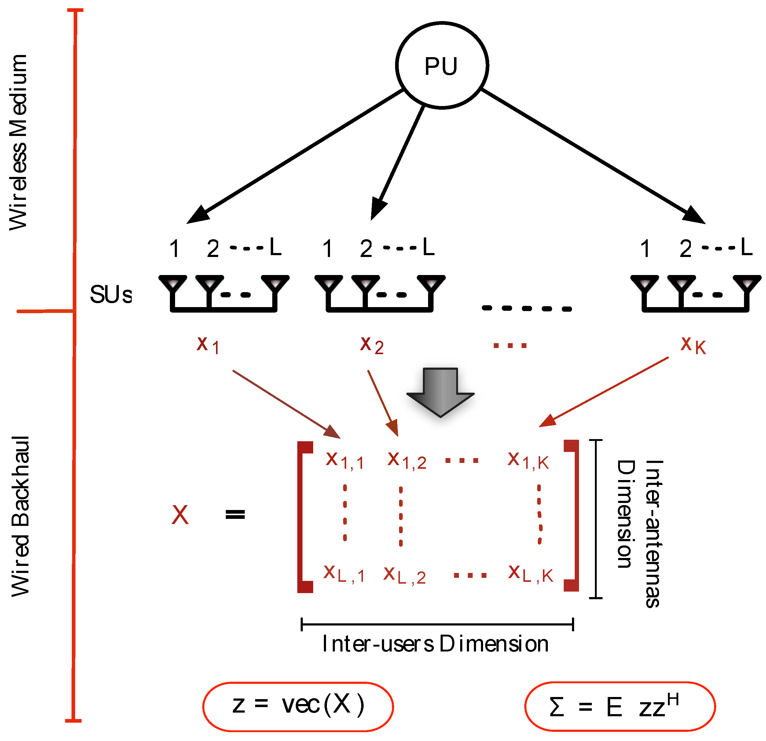
i.e., the base station) via dedicated links. Which is in general a reasonable assumption, as in most of the cases SUs and the fusion center would have mutually agreed upon digital communication links. Moreover, the SUs will have better error correction schemes to overcome the impairments of their corresponding channels with the fusion center. One particular example where such assumption is completely applicable is the cognitive-enabled femtocell networks (network of base stations of femtocells). Femtocells are small cellular telecommunications base stations that can be installed in residential or business environments either as single stand-alone items or in clusters to provide improved cellular coverage within a building [
20]. In most cognitive-enabled femtocell networks, there exists a wired back-haul connection between HeNBs (HeNB is the 3GPP’s term for a LTE femtocell or Small Cell) that can be considered as an ideal link between receivers and the fusion center [
20], as shown in the
Figure 1. The fusion center stacks the received signal vectors
in the (
) matrix
. By using the
operator as
, the two hypotheses can be represented as:
where
Therefore, we have the covariance matrix
as:
where the covariance matrices
,
capture the inter-antennas correlation present in the signal received at
L antennas of the
k-th SU. Similarly, non-zero off-diagonal blocks
with
indicate the presence of inter-receiver spatial correlation. Furthermore, in most practical working conditions, it seems reasonable to consider the ensemble vectors
to be zero mean complex Gaussian distributed, a case that is particularly well-suited for orthogonal frequency division multiplexing (OFDM) [
21]. It is to be noted that we begin with the complex baseband signal sampled at the specific Nyquist rate. Hence, the hypotheses become:
where
, denotes the complex Gaussian distribution with zero mean and covariance
. Under
,
is an unknown diagonal matrix, since in the absence of the primary signal the observations are assumed to be white. Therefore, the detection problem (6) distinguishes a perfectly white noise from spatially correlated (
i.e., inter-receiver and inter-antenna correlation) signal. For this problem, we will next present the traditional detector, and then derive the proposed improved detector by introducing the pair Kronecker product.
Figure 1.
Multi-sensor with Multi-antenna (MAMS) methodology.
Figure 1.
Multi-sensor with Multi-antenna (MAMS) methodology.
3. GLRT Based Detection Scheme
In this section, we adopt the GLRT for the detection problem introduced in Equation (6) since it is asymptotically an optimal detector and it is well-suited to the presence of unknown parameters. Later on, we will use it as a benchmark for the proposed techniques. For the detection problem (6), the GLRT statistic becomes:
where
γ is the threshold,
and
are likelihood functions under hypothesis
and
, respectively. Similarly, the (
) matrix
contains all of the available samples of
,
. Solving Equation (7) we get the final expression of the GLRT as:
where
is the maximum likelihood estimator (MLE) of
. Similarly, under the alternate hypothesis, we assume that only noise is present and
is diagonal matrix, then
. In practice, the GLRT is used based on the assumption that the sample size
N is large while the sample dimensions
are small. However, when the sample support is limited (in particular, when
) , the GLRT degenerates due to the ill-conditioning of the estimated covariance matrix [
22]. A way to reduce these limitations will be presented next.
5. Numerical Results
For the analysis to be conducted herein, we consider a wireless network with a total of
multi-antenna SUs randomly deployed to detect a PU that appears at an unknown position. The spatial correlation between the antennas of a SU is modeled herein as
, with
. Moreover,
with
, which is called correlation coefficient between two adjacent antennas, and it relies on the angular spread
κ, the wavelength
and the distance
d between two adjacent antennas [
12]. Finally, the spatial correlation between SUs due to the correlated shadowing effects is modeled based on the model given in [
26].
In order to analyze the performance of the proposed detectors, we use receiver operating characteristic curve (ROC) and area under the ROC curve (AUC), which varies between 0.5 (poor performance) and 1 (good performance). Moreover, we define the average signal-to-noise ratio (SNR) of all SUs as:
and the SNR of
i-th SU is
where
is the minimum SNR among those of the SUs [
13]. For a given average SNR
and SNR gap
ζ, we can generate the random SNRs of the SUs. Similarly, in order to analyze the effect of noise power uncertainty we generate the noise power at
k-th SU as
, where
, and
means no noise uncertainty.
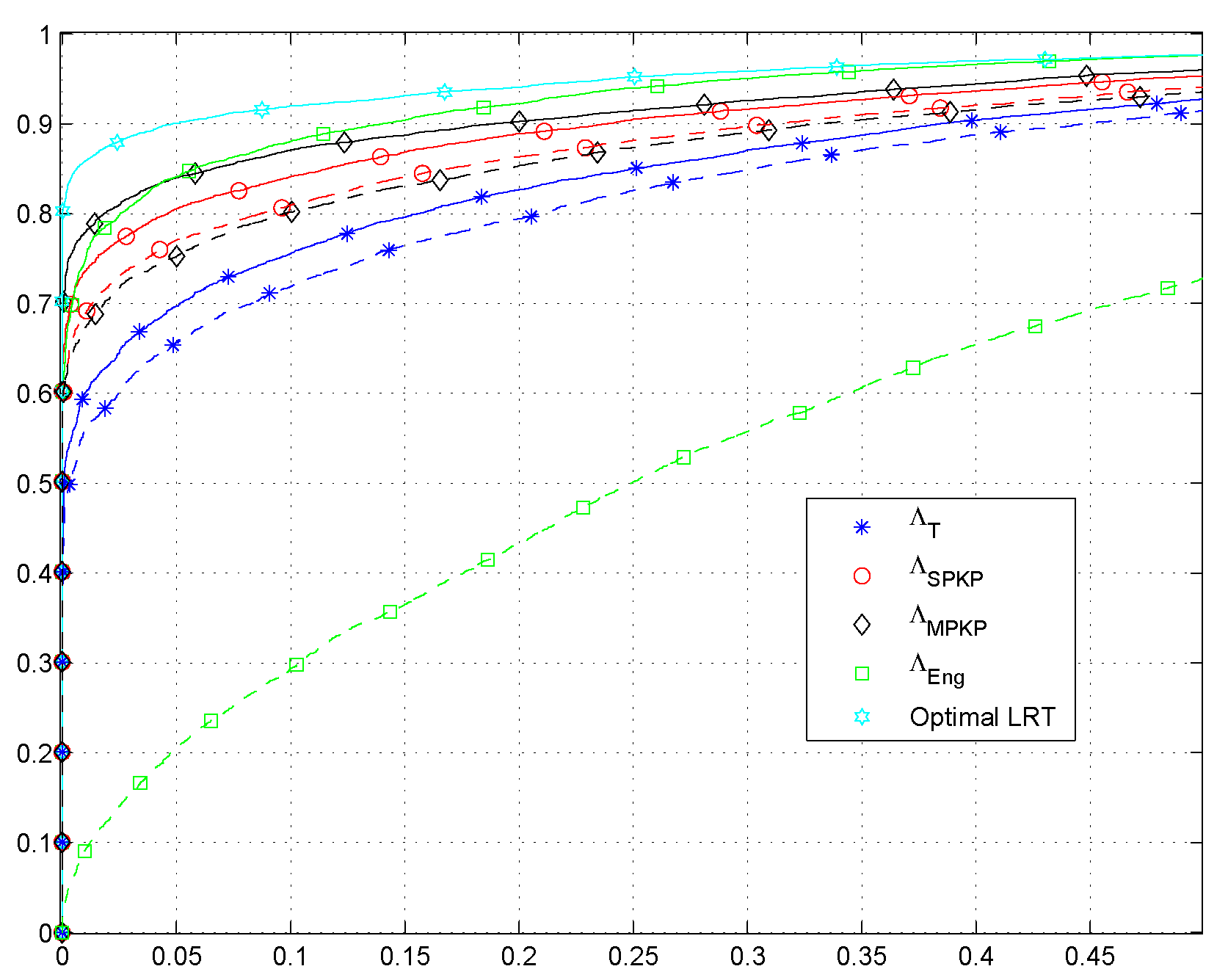
In
Figure 2 we plot ROC curves to compare the performance of our proposed spectrum sensing schemes with the optimal likelihood ratio test (LRT) and the energy detection schemes. For the the optimal LRT, to solve Equation (6) we assume that the covariance matrices under both hypothesis are known. On the other hand the energy detector is given as:
Note that dashed lines represent the plots for
and solid lines represent the case when
. In
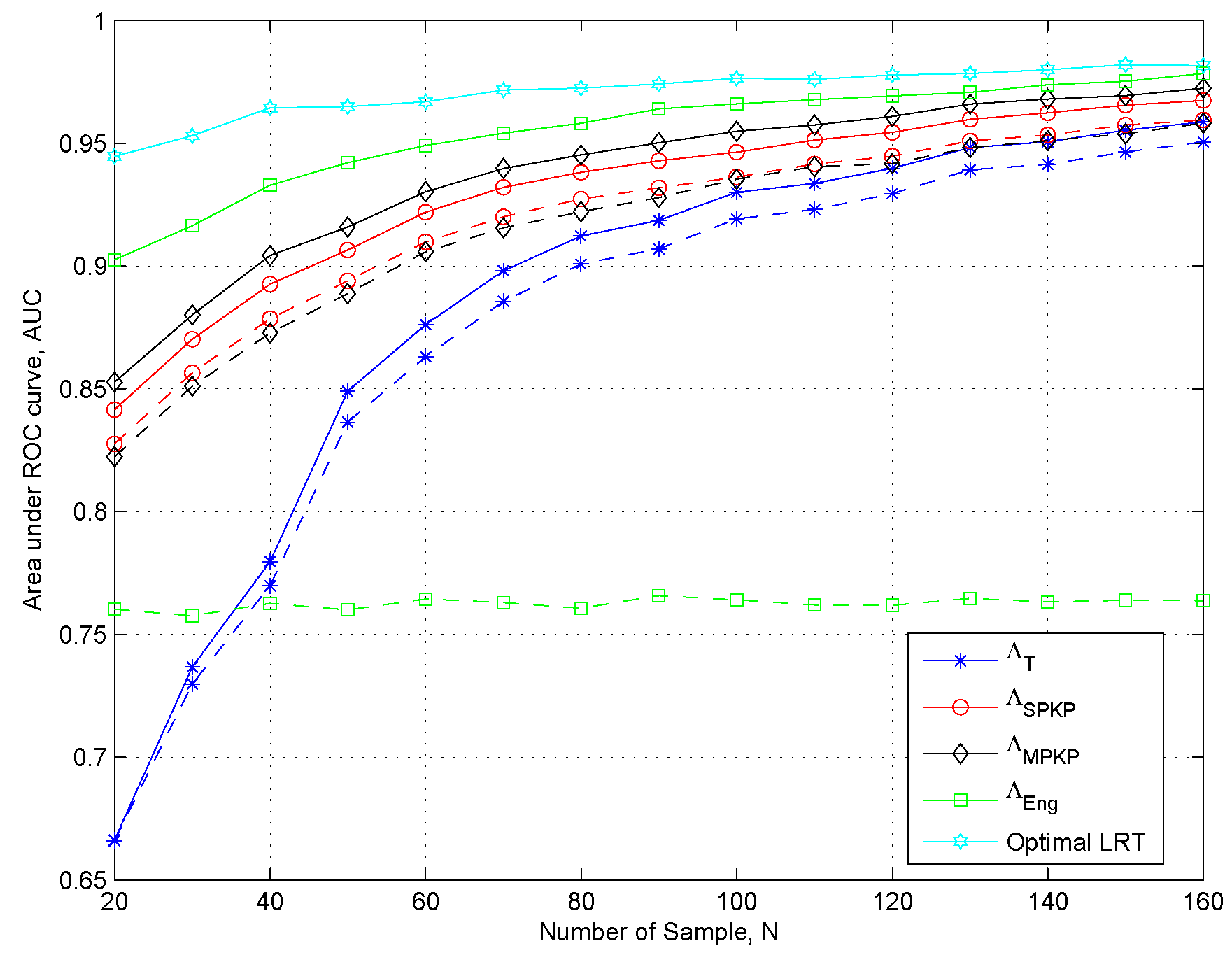
Figure 3, we show the AUC plots to analyze the effects of the sample size
N in the presence of noise power uncertainty. With these considerations, the results clearly show that
and
outperform the traditional GLRT
with a smaller sample support. Moreover, we can see that the energy detector performs better in the absence of the noise power uncertainty, however, it has poor performance in the presence of noise power uncertainty. Interestingly, we can also observe that in the presence of noise power uncertainty, the increase of sample size has very negligible impact on the performance of the energy based detection scheme
due to the phenomena of SNR-Wall [
4]. In
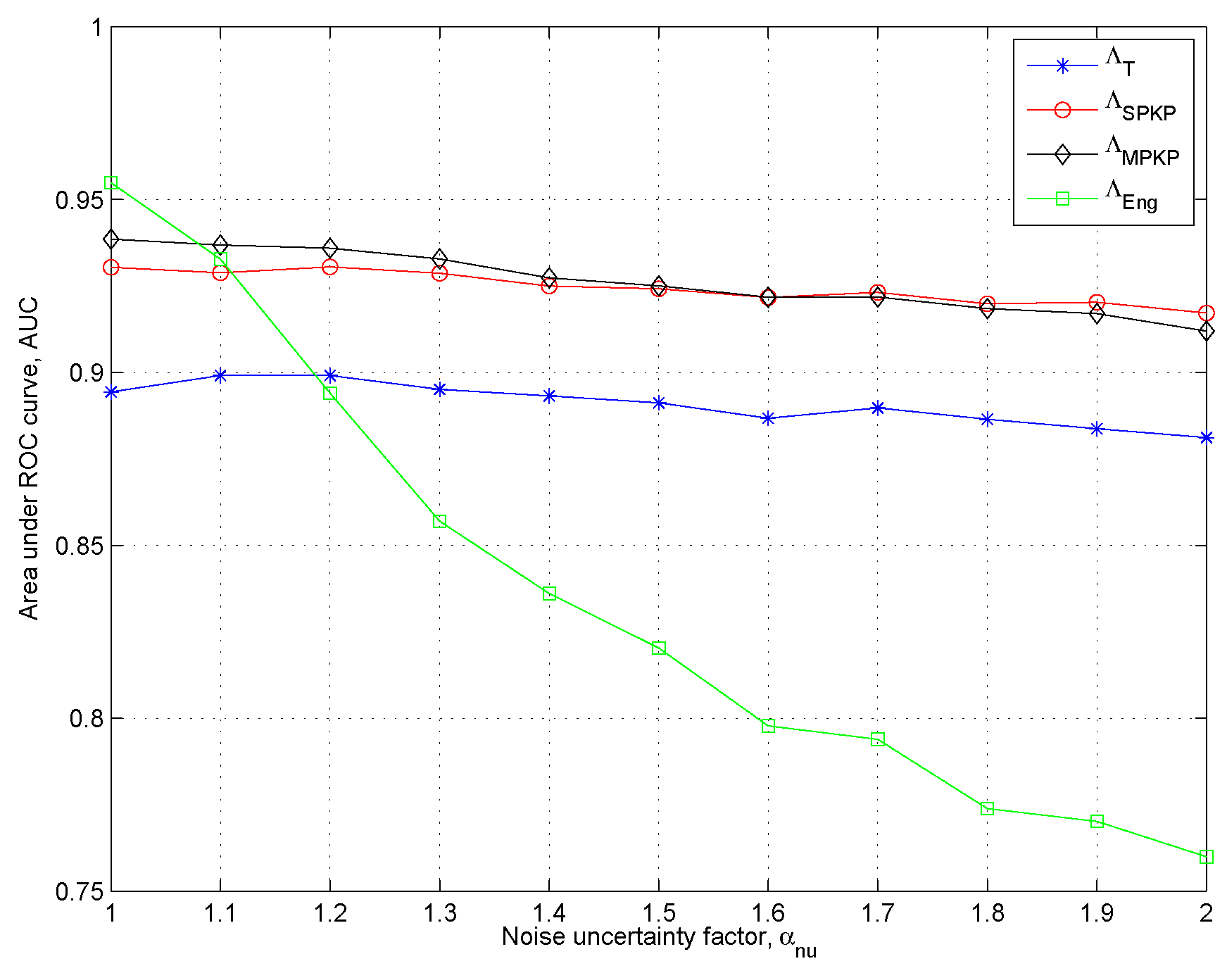
Figure 4, we show the AUC plots to further analyze the effects of noise power uncertainty. Once again, we can see that
and
have superior performance than
and
. Moreover, we can observe the proposed schemes are robust against the noise power uncertainty compared to
. It because the proposed schemes estimate the noise power in real time.
Figure 2.
Receiver operating characteristic (ROC) curves: L = 4, K = 10, N = 70, κ = −15 dB. Solid Lines and Dashed Lines αnu = 2.
Figure 2.
Receiver operating characteristic (ROC) curves: L = 4, K = 10, N = 70, κ = −15 dB. Solid Lines and Dashed Lines αnu = 2.
Figure 3.
Area under the ROC curve to asses the effects of the sample size N, using, κ = −15 dB. Solid Lines αnu = 1, Dashed lines αnu = 2.
Figure 3.
Area under the ROC curve to asses the effects of the sample size N, using, κ = −15 dB. Solid Lines αnu = 1, Dashed lines αnu = 2.
Figure 4.
Area under the ROC curve to asses the effects of Noise uncertainty αnu = 2, N = 70, κ = −15 dB.
Figure 4.
Area under the ROC curve to asses the effects of Noise uncertainty αnu = 2, N = 70, κ = −15 dB.
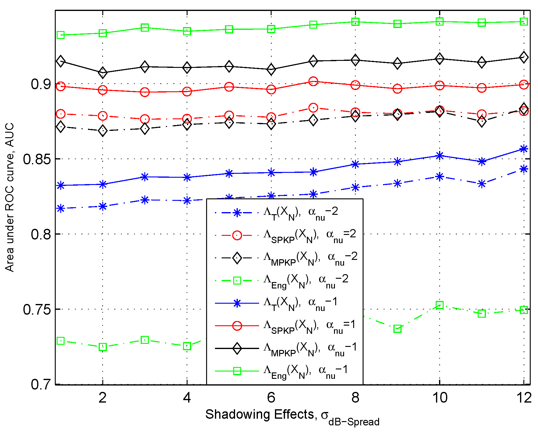
In
Figure 5, we show the AUC plots to analyze the effect of shadowing (
i.e.,
). From the result we can see that the effect of the shadowing is very small over the detection performance of the detection schemes as the presented spectrum sensing schemes are cooperative. However, in the case of
, the detection performance slightly increases with the increase in the
. The most obvious reason for this can be the heavy-tailed distribution of the primary signal strength due to the log-normally-distributed shadow fading that behave in such a way at lower SNR [
27].
Figure 5.
Area under the ROC curve to asses the effect of Shadowing, σdB–Spread: N = 60, κ = −15 dB and Solid Lines αnu = 1, Dashed lines αnu = 2.
Figure 5.
Area under the ROC curve to asses the effect of Shadowing, σdB–Spread: N = 60, κ = −15 dB and Solid Lines αnu = 1, Dashed lines αnu = 2.
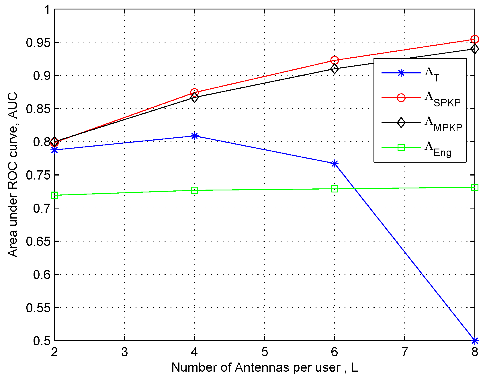
In
Figure 6 and
Figure 7, we show the AUC plots to analyze the effect of number of antennas (
i.e.,
L) for a fixed number of users
K. The results clearly show that the performances of the two proposed schemes are consistently better than the traditional schemes that confirm result in previous plots. However, we can see that the traditional GLRT
performance degrades by increasing L (
i.e.,
to
). It is because for fixed
when
, we have
and we get ill-conditioned sample covariance matrix needed for implementation of GLRT. One the other hand, once again the results in these figures prove that
and
are robust against the issue of large dimensional data and small sample support.
Figure 6.
Area under the ROC curve to asses the effect of number of antennas: N = 60, κ = −15 dB and αnu = 1.
Figure 6.
Area under the ROC curve to asses the effect of number of antennas: N = 60, κ = −15 dB and αnu = 1.
Figure 7.
Area under the ROC curve to asses the effect of number of antennas: N = 60, κ = −15 dB and αnu = 2.
Figure 7.
Area under the ROC curve to asses the effect of number of antennas: N = 60, κ = −15 dB and αnu = 2.
Finally, in order to further analyze the detection performance of the proposed schemes, for a fixed value of probability of false alarm (
), in
Figure 8 we compare the results by plotting probability of detection
vs. average SNR. Once again, we can observe that the proposed schemes
and
outperform the remaining detection schemes presented in this paper.
Figure 8.
PD vs average signal-to-noise ratio (SNR): Number of sensors K = 10, number of antennas L = 4, N = 100 and αnu = 1.
Figure 8.
PD vs average signal-to-noise ratio (SNR): Number of sensors K = 10, number of antennas L = 4, N = 100 and αnu = 1.


