Performance Analysis of Slinky Horizontal Ground Heat Exchangers for a Ground Source Heat Pump System


1
Graduate School of Science and Engineering, Saga University, 1 Honjo-machi, Saga 840-8502, Japan
2
Department of Energy Science and Engineering, Khulna University of Engineering & Technology, Khulna 9203, Bangladesh
3
Department of Mechanical Engineering, Saga University, 1 Honjo-machi, Saga 840-8502, Japan
4
International Institute for Carbon-Neutral Energy Research, Kyushu University, Fukuoka-shi 819-0395, Japan
*
Author to whom correspondence should be addressed.
Resources 2017, 6(4), 56; https://doi.org/10.3390/resources6040056
Submission received: 26 July 2017
/
Revised: 30 September 2017
/
Accepted: 9 October 2017
/
Published: 13 October 2017
Abstract
:This paper highlights the thermal performance of reclined (parallel to ground surface) and standing (perpendicular to ground surface) slinky horizontal ground heat exchangers (HGHEs) with different water mass flow rates in the heating mode of continuous and intermittent operations. A copper tube with an outer surface protected with low-density polyethylene was selected as the tube material of the ground heat exchanger. Effects on ground temperature around the reclined slinky HGHE due to heat extraction and the effect of variation of ground temperatures on reclined HGHE performance are discussed. A higher heat exchange rate was experienced in standing HGHE than in reclined HGHE. The standing HGHE was affected by deeper ground temperature and also a greater amount of backfilled sand in standing HGHE (4.20 m3) than reclined HGHE (1.58 m3), which has higher thermal conductivity than site soil. For mass flow rate of 1 L/min with inlet water temperature 7 °C, the 4-day average heat extraction rates increased 45.3% and 127.3%, respectively, when the initial average ground temperatures at 1.5 m depth around reclined HGHE increased from 10.4 °C to 11.7 °C and 10.4 °C to 13.7 °C. In the case of intermittent operation, which boosted the thermal performance, a short time interval of intermittent operation is better than a long time interval of intermittent operation. Furthermore, from the viewpoint of power consumption by the circulating pump, the intermittent operation is more efficient than continuous operation.
1. Introduction
The conventional sources of energy for heating and cooling of a building have environmental pollution issues. To reduce emissions of carbon dioxide and other greenhouse gases around the world, there is a good opportunity to produce energy from sustainable sources such as solar, wind, biomass, hydro, and ground that produce low or no emissions. In contrast to many other sources of energy for heating and cooling, which need to be transported over long distances, geothermal energy is available on-site. A ground source heat pump (GSHP) transforms this ground energy into useful energy to heat and cool buildings. Even with higher initial cost, GSHPs are the most efficient heating and cooling technology since they use 25% to 50% less electricity [1] than other traditional heating and cooling systems. In order to gain an understanding of how well GSHPs function after installation, analysis of their performance needs to be conducted [2].
In a GSHP system, heat is extracted from or returned to the ground via a closed-loop i.e., ground heat exchanger (GHE) buried in horizontal trenches or vertical boreholes. Horizontal ground heat exchangers (HGHEs) are the common choice of GHEs for small buildings if there are no major limitations on land since they require a larger area in comparison with vertical borehole heat exchangers. HGHEs are usually laid in shallow trenches at a depth of 1.0 to 2.0 m from the ground surface [3,4,5,6]. The performance of GSHP strongly depends on the GHE performance. Therefore, for improving the overall efficiency of GSHPs, the heat transfer efficiency of GHE needs to be improved by adopting more advanced shapes and devices. The shallow HGHEs give lower energy output than vertical GHEs; it is best to improve the efficiency of HGHEs by selecting different geometries of single pipes, multiple pipes, and coiled pipes. Since single and multiple pipes require the greatest amount of ground area and if land area is limited, slinky or spiral GHEs can be placed vertically in narrow trenches or laid flat at the bottom of wide trenches. These slinky or spiral GHEs may be used in order to fit more piping into a small trench area. Also, employing high thermal conductivity materials for HGHEs and backfilling the shallow trench by moderate sand and soil, the required trench lengths are only 20% to 30% compared to single pipe horizontal GSHPs, but trench lengths may increase significantly for equivalent thermal performance [2]. While the slinky or spiral GHE reduces the amount of land used, it requires more pipes, which results in additional costs. Therefore, slinky ground heat exchangers are the subject of many studies that are both experimental as well as numerical.
The heat transfer between the GHE and adjoining ground depends strongly on the ground type and the moisture gradient [7], and the thermal performance of GHEs is affected by the change of ground temperature [7,8]. Ground temperature is a function of the soil thermal properties such as thermal diffusivity, thermal conductivity and the heat capacity [9]. These properties need to be known to predict the thermal behavior of GHEs. Many researchers concluded that the thermal conductivity of soil, velocity of heat transfer fluid [10,11,12] and pipe thermal conductivity [10] are key factors for the thermal performance of ground heat exchanger. Tarnawski et al. [11] mentioned that the heat transfer process of a GHE depends on the pipe diameter, as well as on the density and specific heat capacity of the heat transfer fluid. Consequently, more accurate soil data will allow the designer to minimize the safety factor and reduce the trench length of HGHE installation.
Although numerous analytical and numerical models have been developed for thermal analyses of slinky HGHEs, only a few experimental analyses of slinky HGHEs have been conducted. Most numerical studies assumed that soil thermal and hydraulic properties are constant [6,13,14]. Wu et al. [15] and Congedo et al. [12] numerically simulated the performance analysis of different slinky HGHEs for GSHPs. Fujii et al. [16] simulated the performance of slinky HGHEs for optimum design. Because of the complexity of slinky heat exchanger configurations, Demir et al. [17] calculated heat transfer through a horizontal parallel pipe ground heat exchanger using a numerical method. Selamat et al. [18] numerically investigated the HGHE operation in different configurations to predict the outlet fluid temperature and heat exchange rate. Chong et al. [19] presented the thermal performance of slinky HGHE with various loop pitch, loop diameter, and soil thermal properties in continuous and intermittent operation by numerical simulation. Their results indicate that the system parameters have a significant effect on the thermal performance of the system. A real scale numerical simulation of the present experimental set-up was done by Selamat et al. [6] to analyze and optimize the thermal performance of different layouts of slinky HGHEs. Thermal performance of slinky heat exchangers for GSHP systems was investigated experimentally and numerically by Wu et al. [13] for the UK climate. They showed that the thermal performance of slinky heat exchangers decreased with running time. Adamovsky et al. [5] experimentally compared linear and slinky HGHEs in terms of the soil temperature, heat flows, and energy transferred from the soil massif, and they determined energy recovery capabilities of the ground massif during the stagnation (off) period. Also, due to the lack of information on the heat exchange capacity and long-term performance of the slinky coils, Fujii et al. [20] experimentally performed long-term tests on two types of slinky coil HGHEs and compared their results. Esen and Yuksel [21] experimentally investigated greenhouse heating with slinky HGHEs. To evaluate optimal parameters of the GHE, the effect of mass flow rate, length, buried depth and inlet temperature of water were examined experimentally and analytically with different horizontal configurations [8]. However, most studies on GHE were carried out for continuous operation, and some researchers [19,22,23,24] also investigated the performance of GHE in intermittent operations. The results indicated that the intermittent operations are successful to improve the thermal performance of GHE compared to continuous operations.
In the present work, experimental investigations have been performed to analyze the performance of slinky HGHEs in the heating mode of continuous and intermittent operations. In order to compare the thermal performance of the slinky HGHEs, the GHEs were installed at a depth of 1.5 m in the ground with two orientations: reclined (parallel to ground surface) and standing (perpendicular to ground surface). Water was considered as the working fluid. Thermocouples were installed in different loops of reclined GHE at 0.5 m, 1.0 m and 1.5 m depths to monitor and analyse the ground temperature behavior with the operation time. In addition, to understand the undisturbed ground temperature distribution, thermocouples were placed at different depth positions up to 10 m depth between the two orientations (reclined, standing) of GHEs. At the same time, atmospheric air temperature was also measured.
2. Description of the Experimental Set-Up
2.1. Material Selection and Ground Soil Characteristics
High-density polyethylene (HDPE) tube is a recommended choice in terms of performance and durability for GHEs. However, copper tubing has been successfully used in some applications since copper tubes have a very high thermal conductivity. Regardless of the high thermal conductivity, copper tubes do not have the durability and corrosion resistance of HDPE [2]. Hence, the copper tubing has to be protected from corrosion. Low density polyethylene (LDPE) has similar properties to HDPE, but LDPE is easy to film wrap, which can be used as a surface protection. Furthermore, the analysis [25] shows that the effect of different tube materials is more significant in the slinky configuration of GHE. Therefore, instead of HDPE tubes, which are generally used for horizontal ground heat exchanger, copper tubes protected with a thin coating of LDPE were selected as the tubing of slinky HGHEs in the present study. The present research was conducted at Saga University, Saga City, Japan. The ground sample in the Fukudomi area of Saga city consists of clay from 0 to 15 m in depth, and the water content of 30% to 150% varies with the depth [26]. The thermo-physical properties of GHE tube materials and ground soil are listed in Table 1.
2.2. Details of Experimental Set-Up
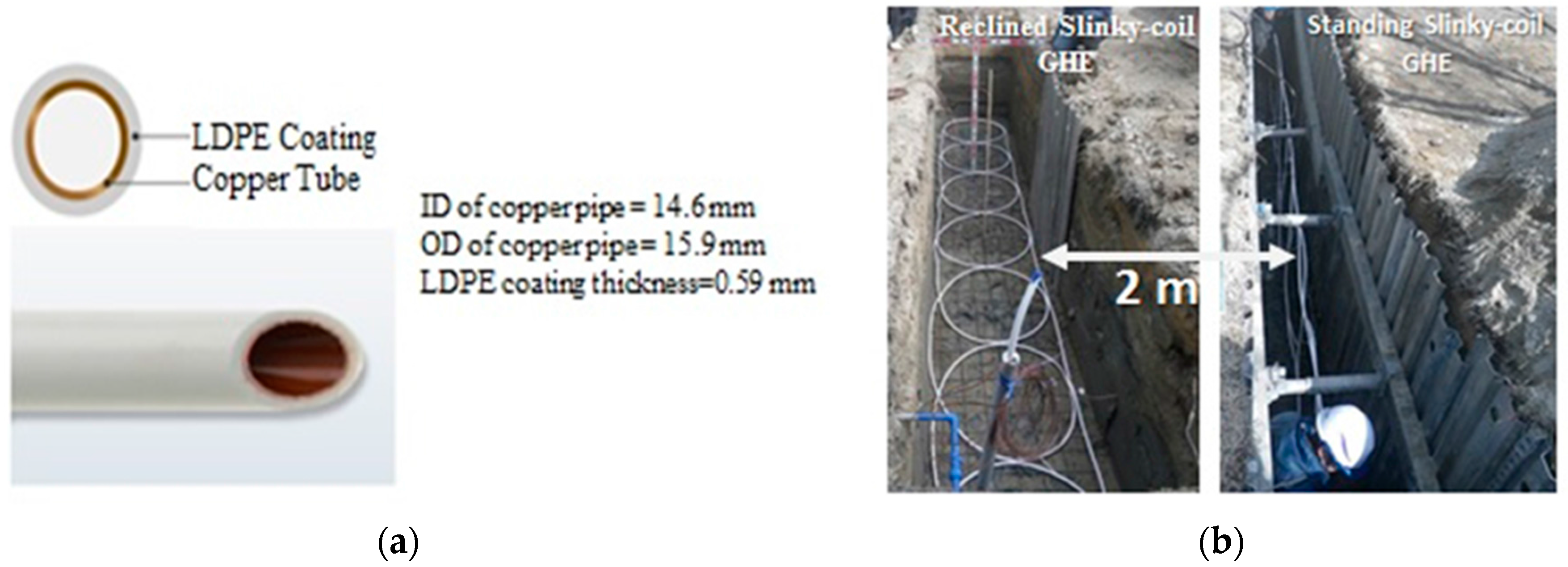
Experimental measurements were conducted in Saga University, Japan, for slinky HGHEs in two orientations: reclined (parallel to ground surface) and standing (perpendicular to ground surface). A schematic diagram of the slinky HGHE system is shown in Figure 1. The reclined and standing slinky HGHEs were installed 2.0 m apart from each other. The copper tube with its outer surface coated with LDPE was considered as the heat exchanger material. The detailed dimensions of the LDPE-coated copper tube is shown in Figure 2a. The loop diameter, length of trench and number of loop for both GHEs are 1.0 m, 7.0 m and 7, respectively. Each GHE consists of 39.5 m in tube length. The reclined GHE was laid in the ground at a 1.5 m depth and 1.0 m wide trench. On the other hand, the centers of standing GHE loops are located at 1.5 m depth and 0.5 m wide trench in the ground. Figure 2b shows the photograph of the installation of both GHEs. After placing the GHEs inside the trenches, the GHEs were covered with typical Japanese sand; water was sprayed on the sand to reduce the void space and hence the thermal resistance around the GHEs. The remaining upper parts of the trenches were then backfilled with site soil and compressed by a power shovel.
Pure water was considered as the heat carrier liquid flowing through the GHEs. The experimental setup also included a water bath (consists of pump, heater & cooler), flow controller, mixing chamber etc. The water bath maintains a constant temperature water supply to the system. The flow controller measures the mass flow rate and also controls the flow rate. The inlet and outlet water temperatures of each GHE were measured using Pt100, which were installed close to the ground surface. In order to obtain a uniform temperature inside the tube, mixing chambers were installed before each Pt100. To monitor undisturbed ground temperature distributions, a monitoring hole in the middle of the two GHEs was dug in the ground to install T-type thermocouples at various depth positions (0.1 m, 0.5 m, 1.0 m, 1.5 m, 2.5 m, 5.0 m, 7.5 m and 10.0 m depth) up to 10.0 m depth. After the installation of thermocouples, the hole was refilled by soil. For the analysis of trench ground temperature variations, T-type thermocouples were placed in the 1st, 4th and 7th loops at 0.5 m, 1.0 m and 1.5 m depth, respectively, of the reclined GHE (shown in Figure 1). At the same time, a digital thermometer was installed about 1.0 m above the ground surface to record ambient temperature. It is also possible to measure the pressure inside the tube by using a pressure sensor. The pressure difference between the inlet and outlet of the GHE is measured by a differential pressure sensor. Data from different measuring points are recorded by a ‘Agilent 34972A’ data logger and stored in a centrally located PC.
2.3. Experimental Data Analysis
To investigate the performance of GHEs, the experimental heat exchange rate is calculated by the following equation:
where is the flow rate of water (kg/s), Cp is the specific heat of water (J/(kg·K)), Ti and To are the inlet and outlet temperatures of water, respectively.
The heat exchange rate per unit tube length of GHE is simplified by the following equation:
where L in the total tube length of GHE.
The overall heat transfer coefficient U is defined by the relation:
where Q is the heat exchange rate (W), U is the overall heat transfer coefficient (W/(m2·°C)), A is the heat transfer area (m2) of GHE, ΔTLM is the logarithmic mean temperature difference (°C).
To calculate the overall heat transfer coefficient from Equation (3) for GHE, the ΔTLM proposed by Naili et al. [8] was adopted as:
where ΔT is the temperature difference between inlet and outlet of GHE (°C), and Tg is the ground soil temperature (°C).
2.4. Uncertainty Analysis
In the present study, the temperatures of water, ground soil and ambient air were measured by Pt100, T-type thermocouple and digital thermometer, respectively. Water mass flow rates were measured by a flow controller. The accuracy of measured data and the results are important issues for the reliability of data and results. Therefore, uncertainty is considered for the experimental measurements. The experimental uncertainties in this study are estimated according Holman (pp. 63–65, [28]). Table 2 summarizes the technical specifications and experimental uncertainties.
If u(xi) is the uncertaninty of independent N set of mesurements in any result represented by R = R(x1, x2, …, xN), then the uncertainity of the result can be calcutated by:
3. Results and Discussion
Based on the experiments of HGHEs in the winter season, the water temperatures in the inlet and outlet, water flow rates and the trench loop ground temperatures of reclined orientation at 0.5 m, 1.0 m and 1.5 m depth were measured for different heating mode. The undisturbed temperatures at various depth positions of ground soil up to 10.0 m depth were also measured. All data were recorded in 5-minute intervals by using a data logger connected to a computer. In addition, the ambient temperature was also measured using a digital thermometer. The experimental conditions in continuous operations are shown in Table 3. All experiments were performed without prior operation of the system.
3.1. Daily Average Ground Thermal Behavior (Undisturbed Ground Temperature)
The temperature distributions in the ground are very important for the performance [21] and sizing of the ground heat exchanger [3]. For the optimum performance of GHEs, it is necessary to know the minimum and maximum ground temperature to decide at which depth the GHE should be installed. Since ambient climatic conditions affect the temperature profile below the ground surface, ambient temperature also needs to be considered when designing a GHE [3]. Consequently, analysis of ground temperature distribution as well as ambient air temperature is required for implementation of GHEs. The ground temperature distribution from 1 February 2016 to 31 March 2017 at various depths up to 10.0 m is shown in Figure 3. This figure also includes the measured ambient temperature.
Figure 3 shows that the ground temperature very close to the ground surface (0.1 m depth) has similar characteristic to ambient temperature and fluctuates strongly and irregularly caused by the change of ambient temperature. Ground temperature fluctuations decrease with increasing ground depth. In the zone 1.0 m to 2.5 m, the ground temperature variation depends mainly on the seasonal weather conditions. Below a certain depth (about 5 m), ground temperature remains relatively constant, about 18 °C at 7.5 to 10.0 m depth, for example. But at the depth 1.5 m where the GHEs were installed in the present study, the ground temperature changes seasonally, which is an important parameter for present GHE performance.
3.2. Comparison of Performance of Standing and Reclined Slinky Horizontal Heat Exchangers
3.2.1. Inlet and Outlet Temperatures of Circulating Water
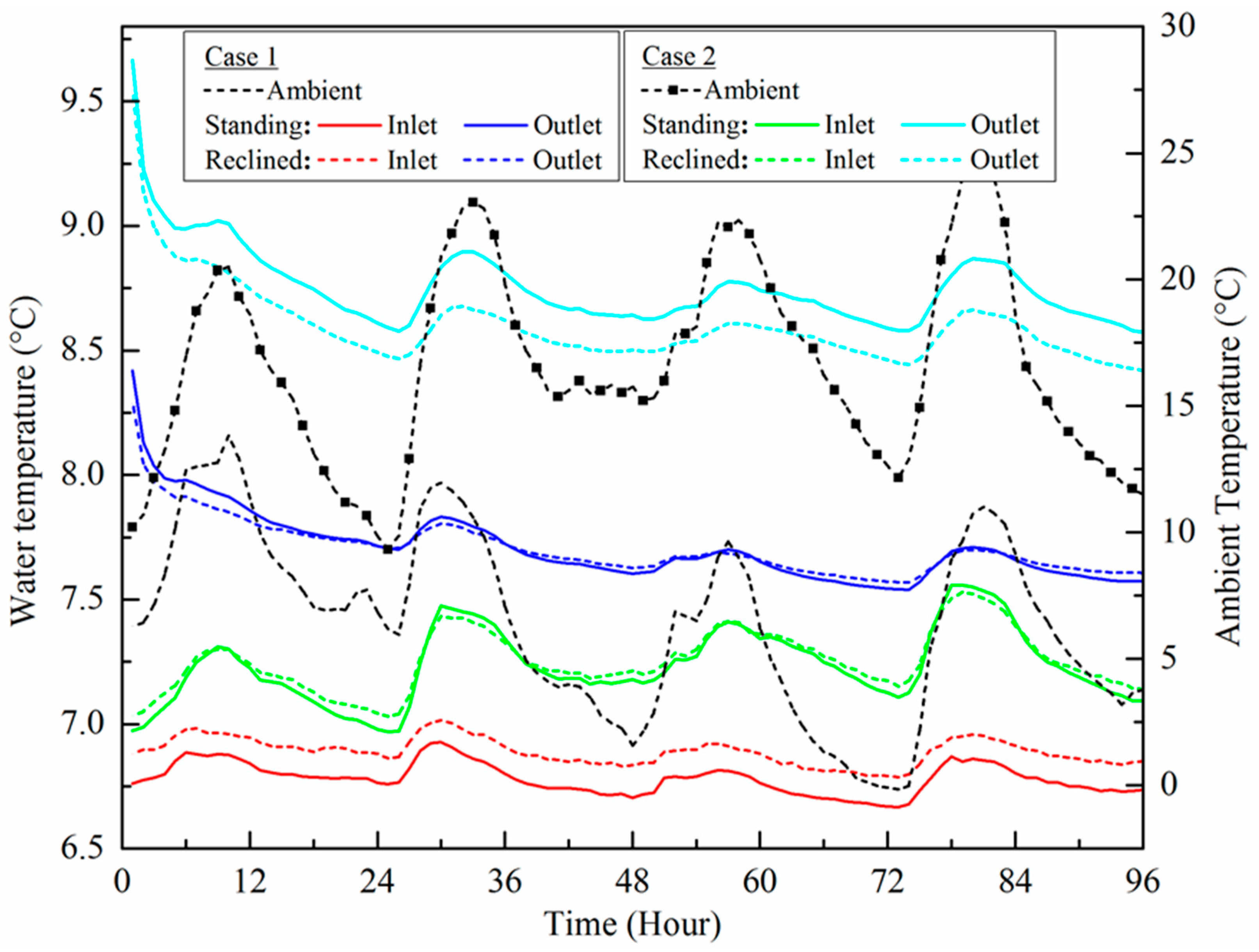
The efficiency of a GSHP system depends on the temperature difference between the inlet and outlet of circulating fluid through the GHE. Therefore, it is desirable to have a higher temperature difference between the inlet and outlet for higher performance of GHEs. The inlet and outlet temperatures for case 1 and case 2 are shown in Figure 4. In case 1 and case 2, the undisturbed ground temperatures between 1.0 m to 2.5 m depth were almost same (Figure 3), with little change. After the start of the experiment, the inlet water temperatures should quickly approach the water bath set temperature (7 °C). At the beginning of the experiment, the outlet temperatures of water are high for both cases 1 and 2 and gradually decrease. The outlet temperatures approach a nearly stable value after about 12 h of operation. Then, there are no significant changes in outlet temperatures for both GHEs, and the experiments were continued until 4 days of continuous operation to observe the steady state performances of GHEs.
For the same operating condition, the standing GHE showed a greater temperature difference between the outlet and inlet than the reclined oriented GHE for both operation periods. After 4 days of operation, the temperature differences between the outlet and inlet of the standing and reclined GHEs are 0.84 °C and 0.76 °C, respectively, for case 1. For case 2, the temperature differences between the outlet and inlet of the standing and reclined GHEs are 1.48 °C and 1.28 °C, respectively. A higher temperature difference between the outlet and inlet leads to a higher heat extraction rate. In Figure 4, it is also seen that the outlet water temperature is higher for 1 L/min than 2 L/min. The lower mass flow rate reduces the velocity of water inside the tube. Consequently, the convective heat transfer coefficient inside the tube as well as the overall heat transfer coefficient decreased. Consequently, the heat extraction will be lower for lower mass flow rate. The effects of lower heat extraction reduce the degradation of ground soil temperature around the GHE. The higher change in water temperature is affected by this low degraded ground soil temperature. As a result, the outlet water temperature is higher with a lower mass flow rate. For instance, the outlet temperatures of the standing GHE with mass flow rates 1 L/min and 2 L/min are 8.57 °C and 7.57 °C, respectively, after 4 days of operation.
The set temperatures of the supply water bath were 7.0 °C for both GHEs, but inlet temperatures fluctuate in a similar fashion as the ambient temperature. The water baths were inside the laboratory room, and the GHE inlet and outlet temperature measuring points were outside the room. The distance between the water bath and measuring point of the water temperature was about 10.0 m. All connecting pipes between water bath and GHEs were insulated, but it is difficult to ensure 100% perfect insulation. Therefore, some heat exchanged between the connecting pipes and surroundings. From Figure 4, it is shown that the inlet temperature fluctuated similarly as the ambient temperature, as well as the outlet temperature.
3.2.2. Heat Exchange Rate
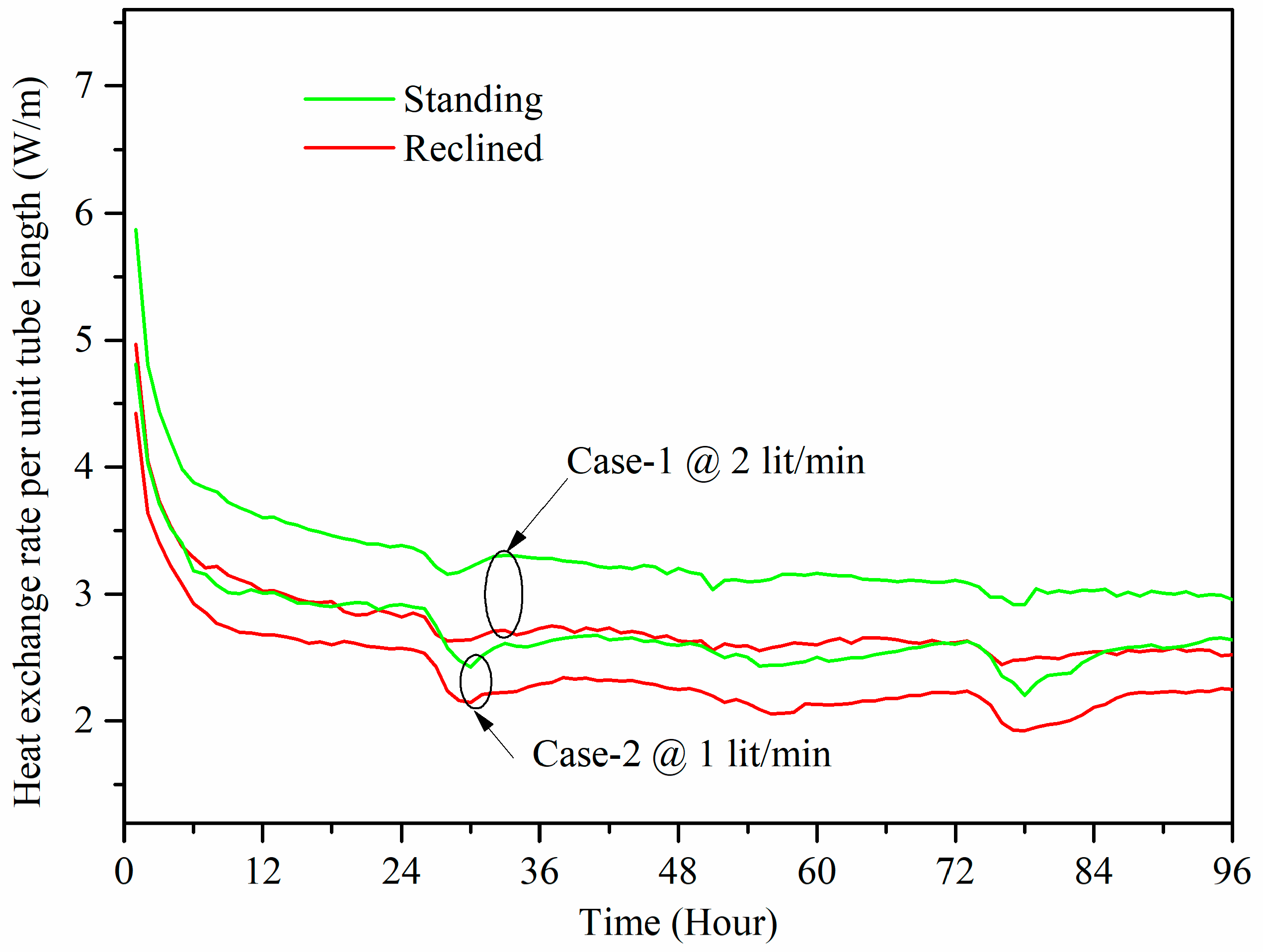
Figure 5 shows the heat exchange rates per unit tube length of the standing and reclined GHEs for cases 1 and 2. At the beginning of the experiments, the heat exchange rates per unit tube length of standing and reclined GHE are high for both cases. This happens due to the higher temperature difference between ground soil around the GHE and circulating water at the beginning. After about 12 h of operation, the heat exchange rate declines slightly and tends to be constant. The reason is because with increases in the operation time, the heat extraction from the vicinity of GHE occurred. As a result, the surrounding ground soil thermal energy degraded and decreased the temperature difference between the soil around the GHEs and the circulating water inside the GHE.
There is a little change in the undisturbed ground soil temperatures during cases 1 and 2. For more comparable of cases 1 and 2, the overall heat transfer coefficient (UA-value) has been calculated using Equation (3). The 12 to 96 h average heat exchange rates and UA-value of cases 1 and 2 are presented in Table 4 for when the system had almost reached the equilibrium (12 h after starting the operation). It can be seen that the heat exchange rate and the overall heat transfer coefficient of standing GHE dominate the heat exchange rate and the overall heat transfer coefficient of the reclined GHE in both cases. For example, the average heat exchange rate and overall heat transfer coefficient (from 12 to 96 h operation) of the standing GHE are 3.17 W/m and 42.66 W/°C, respectively, during case 1. On the other hand, for the reclined GHE, the average heat exchange rate and overall heat transfer coefficient are 2.66 W/m and 35.58 W/°C, respectively, for case 1. The average heat exchange rate of the standing GHE is 19.1% higher than that of the reclined GHE during case 1. During case 2, the average heat exchange rate of the standing GHE is 16.0% higher than that of the reclined GHE.
From the ground temperature distribution in Figure 3, it is seen that ground temperatures at 1.0 m deep and below remained almost constant for a short period of time, 4–5 days, for example. However, the ground temperature in deeper regions is higher than that of shallower regions in the winter season. As the standing GHE was positioned between 1.0 m to 2.0 m vertical depth, half of the standing GHE lay underneath the depth of the reclined GHE. In addition, from Figure 3, it can be seen that the deeper half of the standing GHE was affected by higher temperature than the shallower half. Hence, the standing slinky HGHE was affected by the higher ground temperature in the deeper region. This is one reason why a standing slinky HGHE has a higher heat exchange rate. Also, in the present study, after placing the slinky coils inside the trenches, for the standing GHE, 1.2 m × 0.5 m × 7 m = 4.20 m3 trench volume was backfilled by typical Japanese sand. On the other hand, for the reclined GHE, 0.225 m × 1 m × 7 m = 1.58 m3 volume of trench was backfilled by the same type of sand. The remaining upper parts of the trenches of both GHEs were backfilled by site soil. Hamdhan and Clarke [29] confirmed that the thermal conductivity varies with material condition and soil’s thermal conductivity and was significantly influenced by its saturation and dry density. The thermal conductivity of clay and sand with 20% water content is 1.17 and 1.76, and at a water content of 40%, the conductivity values are 1.59 and 2.18 W/(m·K), respectively [30]. Since the backfill volume of sand is higher for the standing GHE (4.20 m3) than for the reclined GHE (1.58 m3) and the thermal conductivity of sand is higher than that of soil, this may be another reason for the higher heat exchange rate of the standing GHE than the reclined GHE. The installation of slinky HGHEs consists of only piping and excavation work. Though piping of both GHEs is the same, the excavation work differs, as 1 × 1.5 × 7 = 10.5 m3 is required for reclined orientation and 0.5 × 2 × 7 = 7.0 m3 for standing orientation. In contrast to the excavation work, the standing GHE is cost effective.
Figure 5 also shows that the heat exchange rate for case 1 is greater than that for case 2. This is obviously due to increasing mass flow rate, which increases the velocity of water inside the tube. As a result, both the convective heat transfer coefficient and overall heat transfer coefficient UA-value increased. Consequently, with higher mass flow rate, the heat exchange rate is also higher. For the standing GHE, the average heat exchange rate of case 1 is 21.5% higher than that of case 2. The average heat exchange rate for the reclined GHE is 18.2% higher in case 1 than in case 2. Even though the ground temperature changes from case 1 to case 2, this result is comparable because the changes in average ground temperature are small (about 0.25 °C), and the GHE heat exchange rate is always dominated by low thermal conductivity of ground soil.
3.3. Effect of Heat Extraction on Ground Temperature around GHE with the Reclined Slinky HGHE
To understand how the ground temperature around the GHE is changed with the heat exchanged by GHE, the reclined slinky GHE is considered for analysis. The ground temperature distributions of loop 1, 4 and 7 around the reclined GHE at 0.5 m, 1.0 m and 1.5 m depth () for cases 1 and 2 are shown in Figure 6. Figure 6 also includes undisturbed ground temperature at 0.5 m, 1.0 m and 1.5 m depth as well as ambient temperature . Since the circulating water absorbs heat in the heating mode of operation from surrounding ground, the surrounding ground temperatures around GHE gradually decrease with operation time. Also, when the heat exchange fluid enters the GHE, there is short-term, strong heat extraction in the leading loops rather than the subsequent loops. As a result, the ground temperatures around the leading loops decrease quicker than other subsequent loops.
From Figure 6a–c, the initial trench ground soil temperatures around the GHE at 0.5 m, 1.0 m, and 1.5 m depths are different in the 1st, 4th and 7th loops. The reason is that these three loops are located in different horizontal positions (shown in Figure 1), and the energy potential capacities of loops 1, 4 and 7 are different. Also, the at 0.5 m, 1.0 m and 1.5 m depth are different from undisturbed ground soil temperatures of at 0.5 m, 1.0 m and 1.5 m depth. This might be because the undisturbed temperatures were measured inside the original soil, but the trench was first backfilled by sand and site soil. Therefore, the thermo-physical properties and compactness of undisturbed ground soil and trench ground soil are obviously different. The ground surface is affected by the grasses on the surface and by building shading beside the experimental location. Subsurface variables under the ground at different locations also play an important role in the variation of these temperatures. It is also seen that the at 0.5 m and 1.0 m depths for case 2 are higher than those of the at 0.5 m and 1.0 m depths. This is due to the bare surface and may be due to lower compactness of trench ground soil than undisturbed ground soil. The average ambient temperature is about 18.2 °C, which is higher than the ground soil temperature. As a result, are more sensitive to ambient temperature. Despite the bare surface and lower compactness of trench ground soil, is lower than because is affected by shading from a tree.
From Figure 6a, it can be observed that the changing tendency of trench ground temperatures at 0.5 m depth are almost similar to the undisturbed ground temperature at 0.5 m depth and to ambient temperature for both cases 1 and 2. The change of all of these trench ground temperatures slightly lagging behind the changes in ambient temperature is due to the thermal resistance of the ground material. at 0.5 m depth for case 1 remains almost similar to the initial trench ground temperature until about 40 h of operation. After that, it starts to decrease and is greater than the decreases in at 0.5 m depth. However, from Figure 6b, it is seen that at 1.0 m depth for the whole period of case 1 remains almost constant. Therefore, it can be said that the changes in the 1st loop ground temperature at 0.5 m depth occurred only due to the change in ambient temperature and surrounding subsurface soil temperature. Similarly, the increase in at 0.5 m depth during case 2 occurs only due to the increase of ambient temperature and surrounding subsurface ground soil temperature. Also, it can be seen from Figure 6a that the change in trench ground temperatures at 0.5 m depth in the 4th loop and 7th loop occurs only due to changes in ambient temperature and surrounding subsurface ground soil temperature during both cases 1 and 2, but the impact is different in different loops.
In Figure 6b for case 1, the temperatures at 1.0 m depth remain constant and do not decrease due to heat extraction from surrounding soil by circulating water through the GHE. However, for case 2, the trench ground temperatures at 1.0 m depth gradually increase with running time and display almost similar trends of increases in undisturbed ground temperature at 1.0 m depth. In contrast to the variation in the trench loop ground temperatures at 1.0 m depth during cases 1 and 2, up to 1.0 m depth, which is 0.5 m above the reclined GHE, the trench ground temperature is not affected by GHE heat extraction, or the effect is much smaller than the effect of ambient temperature and surrounding subsurface variables.
From Figure 6c, it is seen that the trench ground temperatures at 1.5 m depth start to decrease from the beginning of the experiments, but remains constant from the start of the experiments for both cases 1 and 2. This is because the measuring points of at 1.5 m depth were located in the ground just outside of the GHE coil surface as shown in Figure 1. On the other hand at 1.5 m depth was measured at the center of the 4th loop. Since the loop diameter is 1.0 m, at 1.5 m depth is located 0.5 m lateral distance from the coil surface of the GHE. As a result, it takes time for thermal energy to be extracted by the GHE from center of the 4th loop. decreases slowly compared to at 1.5 m depth. Decreasing rates of gradually decrease with operation time. This fact indicates that heat is exchanging from the surrounding ground soil to the circulating water. Thus, the ground soil temperature degrades with operation time, and the efficiency of the GHE decreases. On the other hand, at 1.5 m depth starts to decrease at about 18 and 24 h after the start of the experiments for cases 1 and 2, respectively. In case 1, starts to decrease earlier than case 2 because a higher mass flow rate through the GHE causes more heat extraction. For instance, the drop in temperatures is 0.75 °C, 0.32 °C and 0.36 °C, respectively, during case 1. On the other hand, for case 2, the drop in is 0.89 °C, 0.32 °C and 0.42 °C, respectively. Though the mass flow rates for cases 1 and 2 are only 2 L/min and 1 L/min, if the mass flow rate would increase, then there is a possibility that the temperature of the ground around the GHE is affected by GHE heat extraction at longer distances from the GHE coils.
The significant finding from Figure 6 is that the slinky HGHE can be installed with variable intervals of loop pitches or by reducing the loop diameter from the starting loop to the end loop because the impact of temperature degradation decreases from the starting loop to subsequent loops. This has the potential to reduce the excavation work and also the installation land area.
3.4. Effect of Variation of Ground Temperature on Thermal Performance of the Reclined Slinky HGHE
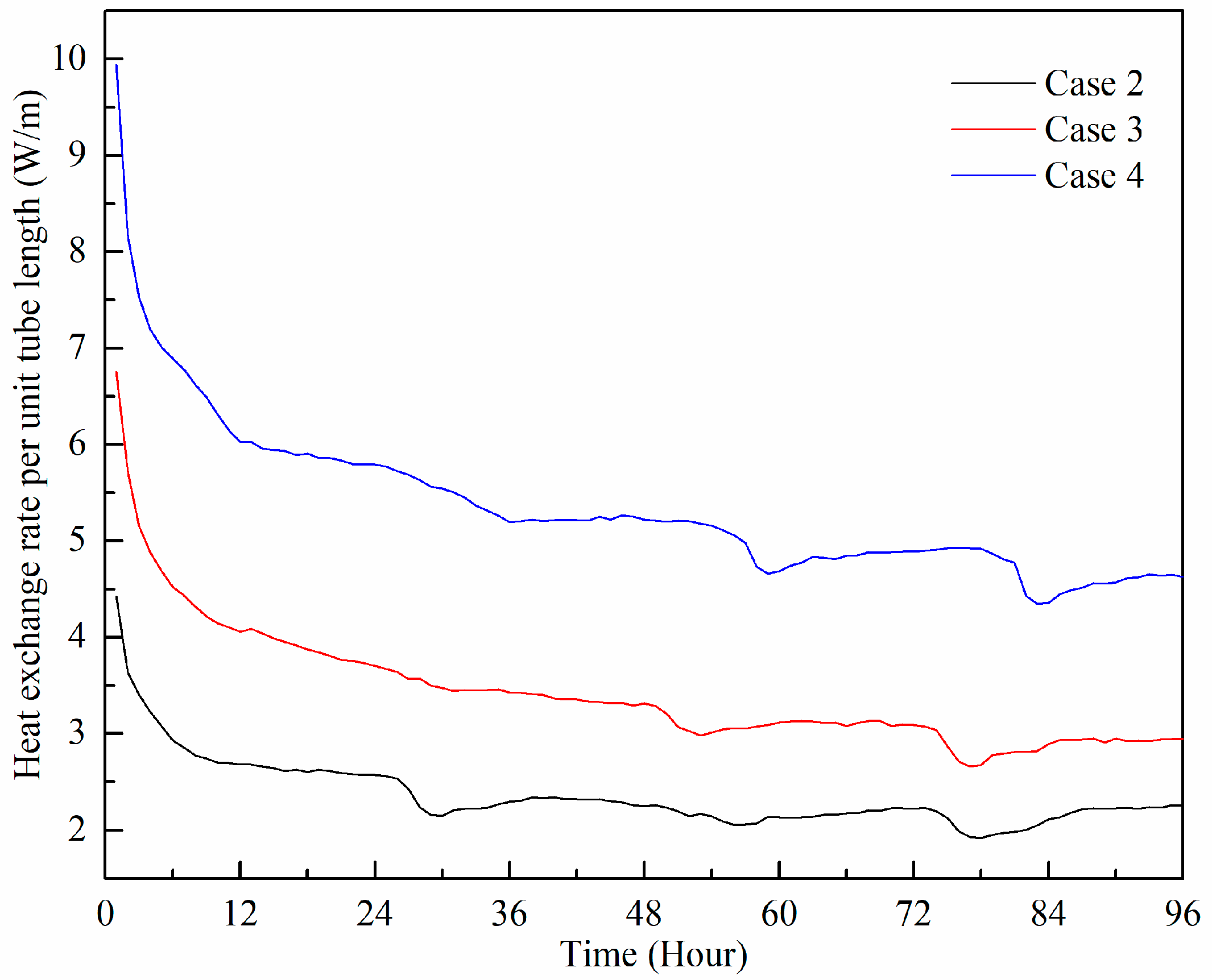
In GHE, there are many factors such as temperature of the ground soil, thermal conductivity, moisture content, rainfall, amount of heat exchange etc. that influence the GHE performance. Therefore, experimental results are compared for different ground soil temperatures with a constant mass flow rate through the reclined HGHE. Figure 7 shows the heat exchange rates for cases 2, 3 and 4. The initial average trench ground temperatures at 1.5 m depth around the GHE are 10.4 °C, 11.7 °C and 13.7 °C. Average heat exchange rates within 4 day from beginning the experiment are 2.36 W/m, 3.43 W/m and 5.36 W/m, respectively, for cases 2, 3 and 4. The average increased heat exchange rates are 45.3% and 127.3% for cases 3 and 4 respectively, compared to case 2. With lower ground soil temperature, the ground becomes saturated quickly (case 2), prone to heat extraction. But when the ground soil temperature is higher, the GHE is capable of continued higher heat extraction (case 3 & 4). It is obvious that the heat extraction rate increases with the increase in ground temperature, but not linearly because the variation pattern of trench ground soil temperature is not similar to the variation of undisturbed ground soil temperature.
For better understanding of the effect of variation in ground temperature on the thermal performance of GHE, Figure 8 shows the temperature distribution of trench ground soil around the reclined GHE and undisturbed ground soil temperature. Figure 8 also includes the ambient temperature and temperature difference of water between the outlet and inlet. The undisturbed ground temperature at 1.5 m depth increases by about 2.9 °C from 4 March to 20 April 2016. However the average values of at 1.5 m depth are 10.4 °C, 10.8 °C and 13.2 °C from 4–7 March, 12–15 March and 17–20 April, respectively.
From Figure 7a–c for cases 2 and 3, it is seen that at 0.5 m depth change almost the same as at 0.5 m depth and . In addition, the variation patterns of at 1.0 m depth are similar to undisturbed ground soil temperature at 1.0 m depth. Therefore, the trench ground soil up to 1.0 m depth might not be affected or only slightly affected by heat extraction in the GHE. However, for case 4, at 0.5 m depth remain almost similar compared to at 0.5 m depth and but not similar to the trend of at 1.0 m depth.
Average temperature differences of water between the outlet and inlet from the beginning of the experiment within 4 days are ΔTcase-2 = 1.4 °C, ΔTcase-3 = 1.9 °C and ΔTcase-4 = 2.8 °C, respectively. Since ΔTcase-4 > ΔTcase-3 > ΔTcase-2, higher heat exchange was experienced in case 4. The at 1.0 m depth are affected by this higher heat exchange in case 4. As the higher heat extraction affects a longer distance around the GHE, attention should be paid to maintain an optimum distance between GHEs for the installation of multiple slinky HGHEs. The behaviors of the drop in at 1.5 m depth for cases 2, 3 and 4 are similar to the discussion pointed out for Figure 6.
Also, from Figure 7b,c, after stopping the experiment in case 3, the average trench ground temperatures at 1.5 m depth on days 1, 2, 3, 4 are 10.5 °C, 10.8 °C, 11.1 °C and 11.3 °C, respectively. On the other hand, the average undisturbed ground temperature at 1.5 m depth on days 1, 2, 3 and 4 is 11.2 °C, 11.2 °C, 11.2 °C and 11.3 °C, respectively. The trench ground temperatures at 1.5 m depth start to increase rapidly after stopping the experiment and continue until about 4 days, after which the trench ground temperature at 1.5 m depth increases gradually similar to the undisturbed ground temperature. Thus, this interval can be considered the heat recovery period of ground soil, but it will depend on the change in undisturbed ground temperature as well as ambient temperature.
3.5. Intermittent Operation of Reclined HGHE
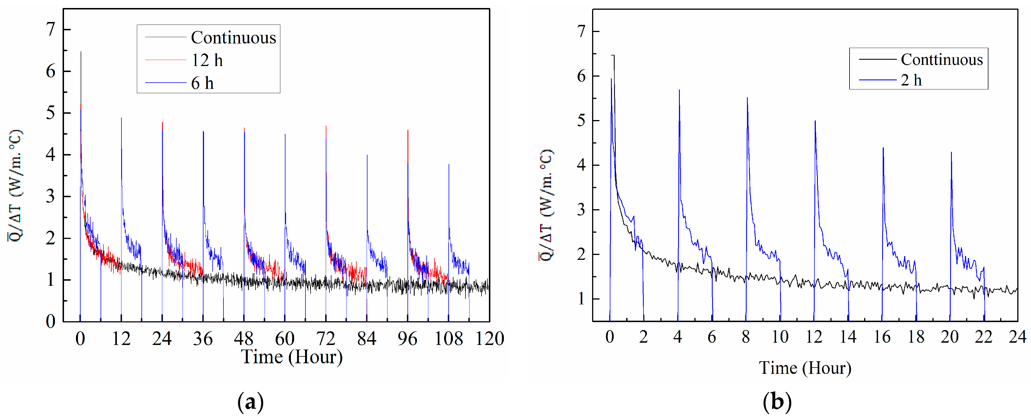
From Figure 5 and Figure 7, it is seen that heat exchange rates of slinky HGHEs are high in the initial 6–12 h and decline gradually. Since HGHEs are installed in shallow ground, the thermal performance is prone to limitation by thermal saturation in the ground region [6] and is affected by ambient air temperature. Selamat et al. [6] concluded that GHEs operate effectively before thermal saturation becomes dominant and suggested that GHEs should operate in cycles or alternate cooling-heating mode to recuperate ground thermal balance. In order to investigate the heat exchange characteristics of GHEs with intermittent operation, the experiments were conducted for different intermittent operations of the heating mode with mass flow rate 4 L/min. The intermittent operations were performed for 12 h, 6 h and 2 h intervals from 10–14 February, 24–28 February and on 6 March 2017, respectively, for the reclined slinky HGHE. Before that, the experiment was performed under continuous operation from 29 January to 2 February 2017 with the same mass flow rate. Then, thermal performances were compared between continuous and different intermittent operations. It was already noticed in Figure 7 that the thermal performance of GHE depends on ground temperature. Fujii et al. [17] introduced a parameter to eliminate this effect. Since in our experiment, the inlet set temperature was fixed to 7.0 °C, we are considering the following parameter for intermittent performance analysis of GHE more accurately:
where is the heat exchange rate per unit tube length, Tg is the undisturbed ground temperature at 1.5 m depth and To is the outlet water temperature of the GHE. This parameter can be called the overall heat transfer response with respect to the change in the temperature difference between undisturbed ground and outlet water. Figure 9 shows the time variation of values for different intermittent operations. It is seen that the for all intermittent operations is significantly higher than for the continuous operations. In the intermittent operation, the off period reduces the effect of heat degradation of ground soil around the GHE; thus, the ground is allowed to recuperate its thermal condition during this off period. The heat regeneration in the off time period contributed significantly to the increase in the heat exchange rate.
In order to observe the benefit of intermittent operation in contrast to continuous operation, the results presented in Figure 9 are integrated and then compared between the continuous and different intermittent operations. The integral of results presented in Figure 9 is calculated by using Equation (7).
where S (W·h/(m·°C)) is the total value of in a cycle; t is the time (h).
Table 5 shows the calculated S values for the continuous and intermittent operations and also includes the integral of the continuous cycle over only the same on-periods of the intermittent operation. It is apparent that the S values (enclosed by ellipses) of the continuous cycle are always higher than those of the intermittent cycle. However, the S values (enclosed by rectangles) of over only the on-periods of a cycle for all of the intermittent operations are always higher than for the continuous operation. Therefore, the merits of the intermittent cycle can be achieved if the integral of the continuous cycle is considered over only the same on-periods of the intermittent operation.
Furthermore, to show the benefits of intermittent operation from the viewpoint of power consumption by the circulating pump, the cycle integral value S can be compared on the basis of pump power consumption to circulate the water through the GHE. The active operation time for all of the intermittent operations is one-half of the continuous operations. Consequently, the pump power consumptions of the intermittent operations are 50% of the continuous operations. Therefore, the S value of any intermittent operation is less than of continuous operation, but not less than 50%. Thus, the intermittent operation is more efficient from the view of the pump power consumption. For example, at 12 h intermittent operation, the S value is 70.4% of the continuous operation. At the same time the, pump power consumption for the intermittent operation is 50% of the continuous operation.
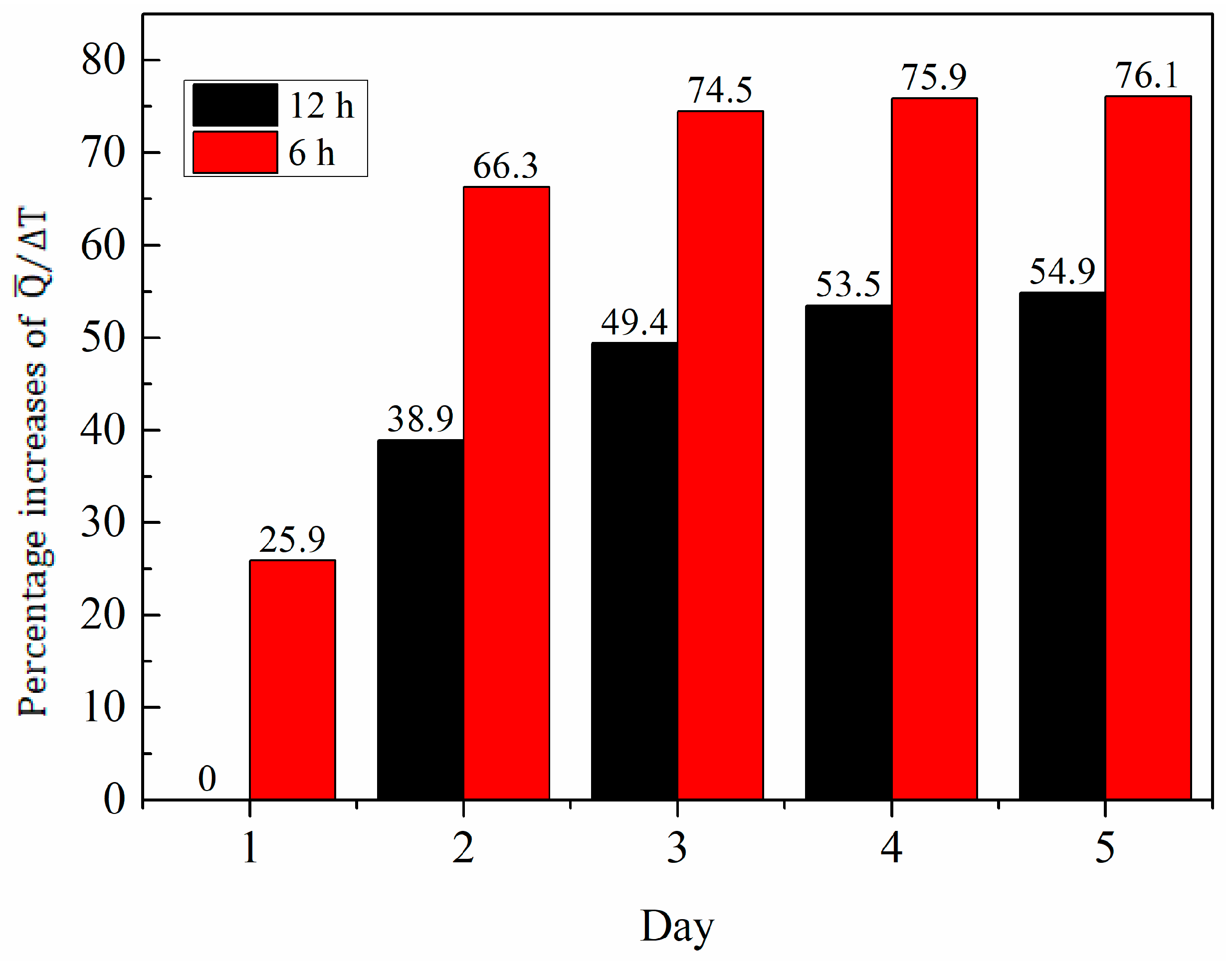
With considering only on-periods of a cycle, Figure 10 shows 12 h average percentage increases in for 12 h and 6 h interval operations based on continuous operation. From this figure, it can be seen that the percentage increases in during 6 h interval operation are higher than those of the 12 h interval operation. For example, the 12 h average of the value increased 66.3% in 6 h and 38.9% in 12 h interval of operations on the 2nd day. In comparison, with respect to the continuous operation, the increased 43.0% and 25.2% for 2 h and 6 h interval operations, respectively, on the first day of operation. The physical significance of is that a higher value indicates a quicker overall heat transfer response. From this comparison, it can be concluded that there is a good opportunity to operate slinky HGHEs in intermittent mode, which will significantly increase the performance. During the off period, supplemental sources (air source, for example) can be used to meet the continuous heat demand.
4. Conclusions
The experimental thermal performances of slinky HGHEs (standing and reclined orientation) have been measured in different heating modes. The experimental results highlighted the comparison of the performances of standing and reclined orientation, effects on ground temperature around the reclined HGHE due to heat extraction, and the effect of variation in ground temperature on reclined HGHE performance. The thermal performance improvements by intermittent operations of GHE are also discussed. Moreover, the temperature distributions of the undisturbed ground and ambient temperature are also measured.
The measured undisturbed ground temperature information provides a useful indicator of the installation of GHEs at a suitable depth for heating and cooling purposes.
A higher heat exchange rate of the standing HGHE compared to the reclined HGHE was observed. The average heat exchange rate is 16.0% higher for the standing slinky HGHE than the reclined slinky HGHE at a flow rate of 1 L/min. For the mass flow rate 2 L/min, the average heat exchange rate of the standing GHE is 19.1% higher than the reclined GHE. In addition, the calculated overall heat transfer coefficient UA-value signifies the customary sizing of slinky GHEs for different ground soil temperatures and operating conditions. It can be suggested that slinky HGHEs in standing orientation would require more significant backfilling by using high thermal conductivity material. With respect to excavation work, standing slinky HGHEs are cost effective compared with reclined slinky HGHEs.
The trench ground temperature variation of different loops around the GHE decreased from starting loop to subsequent loops. Since the impact of the heat exchange rate on ground temperature variation decreases from the starting loop to subsequent loops, slinky HGHEs can be installed with a gradually sinking loop pitch from the starting loop to the end loop. This has the potential to reduce the installation land area as well as the excavation work.
For the mass flow rate of 1 L/min with inlet water temperature 7 °C, the 4-day average heat extraction rates increased 45.3% and 127.3%, respectively, when the initial average ground temperatures at 1.5 m depth around reclined HGHE increased from 10.4 °C to 11.7 °C and 10.4 °C to 13.7 °C. This is not a linear relationship because the variation pattern of the trench ground soil temperature is not similar to the variation in the undisturbed ground soil temperature.
The ground temperature degradation can be recovered by the intermittent operation of the GHE. The intermittent operation exhibited a great potential to boost the thermal performance of the slinky HGHE. From the viewpoint of the overall heat transfer response parameter, a short time interval of intermittent operation is better than a long time interval of intermittent operation. It is apparent that the cycle integral value of for the continuous operation is always higher than that of the intermittent operation. However, the merits of the intermittent cycle can be achieved if the integral of for the continuous cycle is compared over only the same on-periods of intermittent operation. Furthermore, from the viewpoint of power consumption by the circulating pump, intermittent operation is more efficient than continuous operation.
Acknowledgments
This work was sponsored by the project “Renewable energy-heat utilization technology & development project” of the New Energy and Industrial Technology Development Organization (NEDO), Japan.
Author Contributions
All authors conceived and designed the experiments; Md. Hasan Ali performed the experiments; Md. Hasan Ali analyzed the data in cooperation with both of the co-authors; Keishi Kariya contributed to provide materials; Md. Hasan Ali wrote the paper. Akio Miyara provided guidance, supervision and contributed to revision of this paper.
Conflicts of Interest
The authors declare no conflict of interest.
References
- Sarbu, I.; Sebarchievici, C. General review of ground-source heat pump systems for heating and cooling of buildings. Energy Build. 2014, 70, 441–454. [Google Scholar] [CrossRef]
- Kavanaugh, S.P.; Rafferty, K. Ground-Source Heat Pumps, Design of Geothermal Systems for Commercial and Institutional Buildings; ASHRAE: Atlanta, GA, USA, 1997; ISBN 1-883413-52-4. [Google Scholar]
- Florides, G.; Kalogirou, S. Ground heat exchangers-A review of systems, models and applications. Renew. Energy 2007, 32, 2461–2478. [Google Scholar] [CrossRef]
- Chiasson, A.D. Modeling horizontal ground heat exchangers in geothermal heat pump systems. In Proceedings of the COMSOL Conference, Boston, MA, USA, 7–9 October 2010. [Google Scholar]
- Adamovsky, D.; Neuberger, P.; Adamovsky, R. Changes in energy and temperature in the ground mass with horizontal heat exchangers-The energy source for heat pumps. Energy Build. 2015, 92, 107–115. [Google Scholar] [CrossRef]
- Selamat, S.; Miyara, A.; Kariya, K. Numerical study of horizontal ground heat exchangers for design optimization. Renew. Energy 2016, 95, 561–573. [Google Scholar] [CrossRef]
- Leong, W.H.; Tarnawski, V.R.; Aittomaki, A. Effect of soil type and moisture content on ground heat pump performance. Int. J. Refriger. 1998, 21, 595–606. [Google Scholar] [CrossRef]
- Naili, N.; Hazami, M.; Attar, I.; Farhat, A. In-field performance analysis of ground source cooling system with horizontal ground heat exchanger in Tunisia. Energy 2013, 61, 319–331. [Google Scholar] [CrossRef]
- Florides, G.; Theofanous, E.; Iosif-Stylianou, I.; Tassou, S.; Christodoulides, P.; Zomeni, Z. Modeling and assessment of the efficiency of horizontal and vertical ground heat exchangers. Energy 2013, 58, 655–663. [Google Scholar] [CrossRef]
- Song, Y.; Yao, Y.; Na, W. Impacts of soil pipe thermal Conductivity on performance of horizontal pipe in a ground-source heat pump. In Proceedings of the Sixth International Conference for Enhanced Building Operations, Shenzhen, China, 6–9 November 2006. [Google Scholar]
- Tarnawski, V.R.; Leong, W.H.; Momose, T.; Hamada, Y. Analysis of ground source heat pumps with horizontal ground heat exchangers for northern Japan. Renew. Energy 2009, 34, 127–134. [Google Scholar] [CrossRef]
- Congedo, P.M.; Colangelo, G.; Starace, G. CFD simulations of horizontal ground heat exchangers: A comparison among different configurations. Appl. Therm. Eng. 2012, 33–34, 24–32. [Google Scholar] [CrossRef]
- Wu, Y.; Gan, G.; Verhoef, A.; Vidale, P.L.; Gonzalez, R.G. Experimental measurement and numerical simulation of horizontal-coupled slinky ground source heat exchangers. Appl. Therm. Eng. 2010, 30, 2574–2583. [Google Scholar] [CrossRef]
- Xiong, Z.; Fisher, D.E.; Spitler, J.D. Development and validation of a slinky ground heat exchanger model. Appl. Energy 2015, 141, 57–69. [Google Scholar] [CrossRef]
- Wu, Y.; Gan, G.; Gonzalez, R.G.; Verhoef, A.; Vidale, P.L. Prediction of the thermal performance of horizontal-coupled ground source heat exchangers. Int. J. Low Carbon Technol. 2011, 6, 261–269. [Google Scholar] [CrossRef]
- Fujii, H.; Nishia, K.; Komaniwaa, Y.; Choub, N. Numerical modeling of slinky-coil horizontal ground heat exchangers. Geothermics 2012, 41, 55–62. [Google Scholar] [CrossRef]
- Demir, H.; Koyun, A.; Temir, G. Heat transfer of horizontal parallel pipe ground heat exchanger and experimental verification. Appl. Therm. Eng. 2009, 29, 224–233. [Google Scholar] [CrossRef]
- Selamat, S.; Miyara, A.; Kariya, K. Considerations for horizontal ground heat exchanger loops operation. Trans. JSRAE 2015, 32, 345–351. [Google Scholar]
- Chong, C.S.A.; Gan, G.; Verhoef, A.; Garcia, R.G.; Vidale, P.L. Simulation of thermal performance of horizontal slinky-loop heat exchangers for ground source heat pumps. Appl. Energy 2013, 104, 603–610. [Google Scholar] [CrossRef]
- Fujii, H.; Okubo, H.; Cho, N.; Ohyama, K. Field tests of horizontal ground heat exchangers. In Proceedings of the World Geothermal Congress, Bali, Indonesia, 25–29 April 2010. [Google Scholar]
- Esen, H.; Inalli, M.; Esen, M. Numerical and experimental analysis of a horizontal ground coupled heat pump system. Build. Environ. 2007, 42, 1126–1134. [Google Scholar] [CrossRef]
- Benazza, A.; Blanco, E.; Aichouba, M.; Río, J.L.; Laouedj, S. Numerical investigation of horizontal ground coupled heat exchanger. Energy Procedia 2011, 6, 29–35. [Google Scholar] [CrossRef]
- Jalaluddin; Miyara, A. Thermal performance investigation of several types of vertical ground heat exchangers with different operation mode. Appl. Therm. Eng. 2012, 33–34, 167–174. [Google Scholar] [CrossRef]
- Selamat, S.; Miyara, A.; Kariya, K. Analysis of short time period of operation of horizontal ground heat exchangers. Resources 2015, 4, 507–523. [Google Scholar] [CrossRef]
- Selamat, S.; Miyara, A.; Kariya, K. Comparison of heat exchange rates between straight and slinky horizontal ground heat exchanger. In Proceedings of the 24th IIR International Congress of Refrigeration, Yokohama, Japan, 16–22 August 2015. [Google Scholar]
- Hino, T.; Koslanant, S.; Onitsuka, K.; Negami, T. Changes in Properties of Holocene Series during Storage in Thin Wall Tube Samplers; Report of the Faculty of Science and Engineering; Saga University: Saga, Japan, 2007; Volume 36. [Google Scholar]
- Jsme Data Book: Heat Transfer, 5th ed.; The Japan Society of Mechanical Engineers: Saporo, Japan, 2009. (In Japanese)
- Holman, J.P. Experimental Methods for Engineers; McGraw-Hill Education: Singapore, 2012. [Google Scholar]
- Hamdhan, I.N.; Clarke, B.G. Determination of thermal conductivity of coarse and fine sand soils. In Proceedings of the World Geothermal Congress, Bali, Indonesia, 25–29 April 2010. [Google Scholar]
- Hillel, D. Environmental Soil Physics; Academic Press, Imprint of Elsevier: San Diego, CA, USA, 1998; ISBN 978-0-12-348525-0. [Google Scholar]
Figure 1.
Schematic of experimental set-up of slinky horizontal ground heat exchangers.
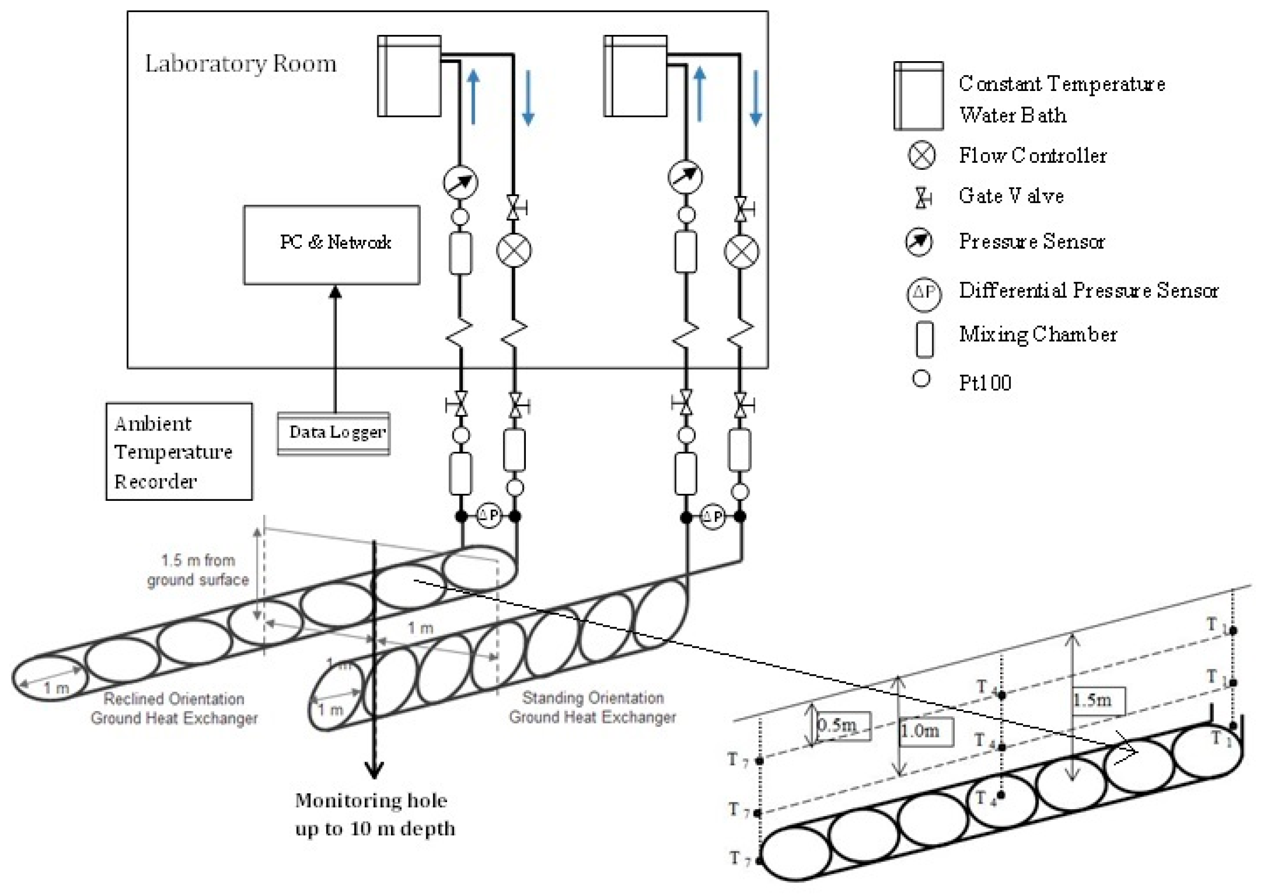
Figure 2.
(a) Outer surface LDPE-coated copper tube; (b) Installation of slinky-coil ground heat exchangers.
Figure 2.
(a) Outer surface LDPE-coated copper tube; (b) Installation of slinky-coil ground heat exchangers.

Figure 3.
Measured daily average ground temperature and ambient temperature from 1 February 2016 to 31 March 2017.
Figure 3.
Measured daily average ground temperature and ambient temperature from 1 February 2016 to 31 March 2017.
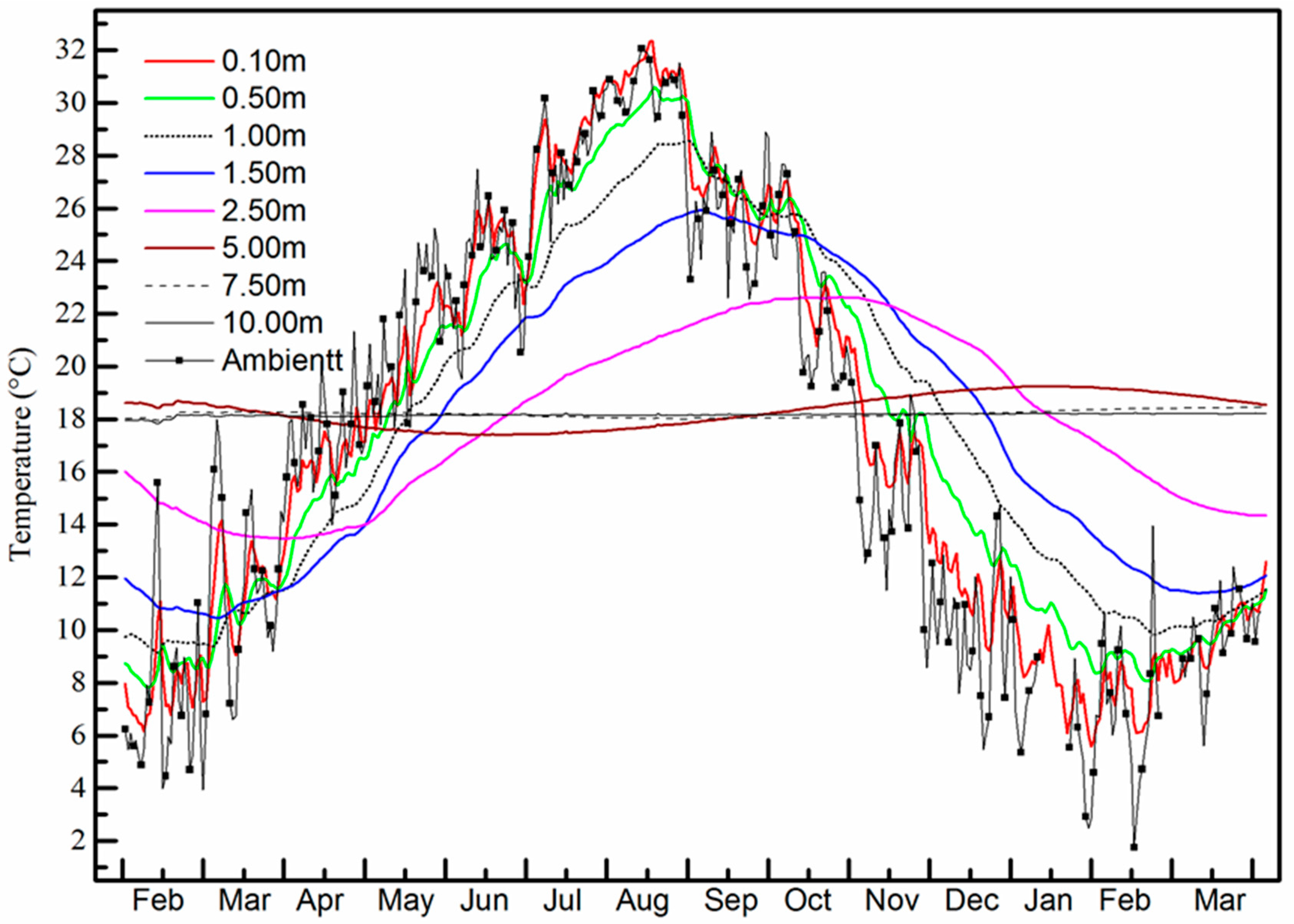
Figure 4.
Time variation of inlet and outlet water temperature and ambient temperature in heating mode during cases 1 and 2.
Figure 4.
Time variation of inlet and outlet water temperature and ambient temperature in heating mode during cases 1 and 2.

Figure 5.
Comparison of heat exchange rate between standing and reclined oriented GHEs for cases 1 and 2.
Figure 5.
Comparison of heat exchange rate between standing and reclined oriented GHEs for cases 1 and 2.

Figure 6.
Variation of ground temperature around the reclined GHE with operation time in different loops and undisturbed ground temperature during cases 1 and 2: (a) at 0.5 m depth and ambient; (b) at 1.0 m depth; (c) at 1.5 m depth.
Figure 6.
Variation of ground temperature around the reclined GHE with operation time in different loops and undisturbed ground temperature during cases 1 and 2: (a) at 0.5 m depth and ambient; (b) at 1.0 m depth; (c) at 1.5 m depth.
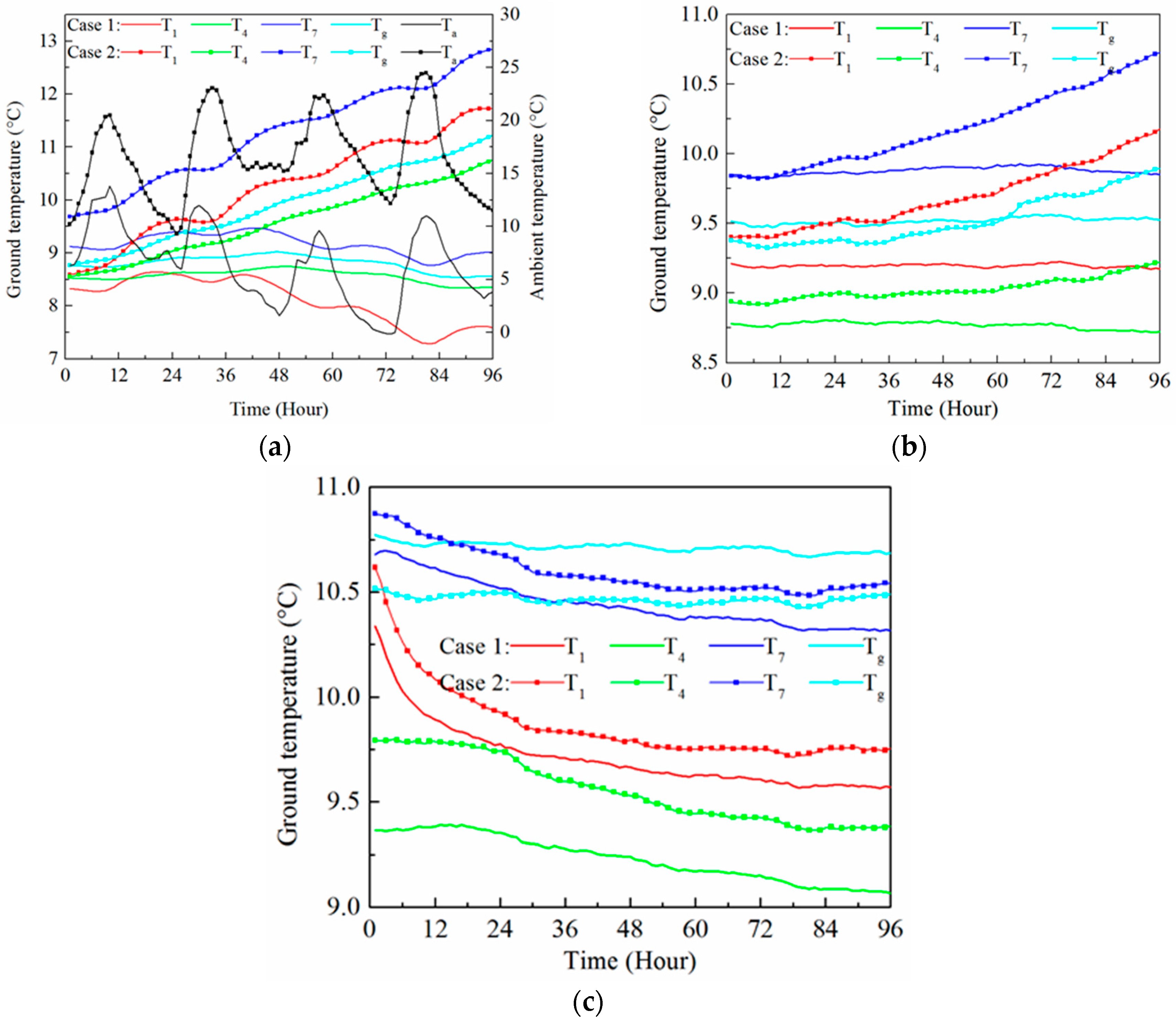
Figure 7.
Heat exchange rate of reclined GHE for cases 2, 3 and 4.

Figure 8.
Variation in ground temperature from 4 March to 20 April 2016 around the reclined GHE and undisturbed ground: (a) at 0.5 m depth and ambient; (b) at 1.0 m depth; (c) at 1.5 m depth and water temperature difference between the GHE outlet and inlet.
Figure 8.
Variation in ground temperature from 4 March to 20 April 2016 around the reclined GHE and undisturbed ground: (a) at 0.5 m depth and ambient; (b) at 1.0 m depth; (c) at 1.5 m depth and water temperature difference between the GHE outlet and inlet.
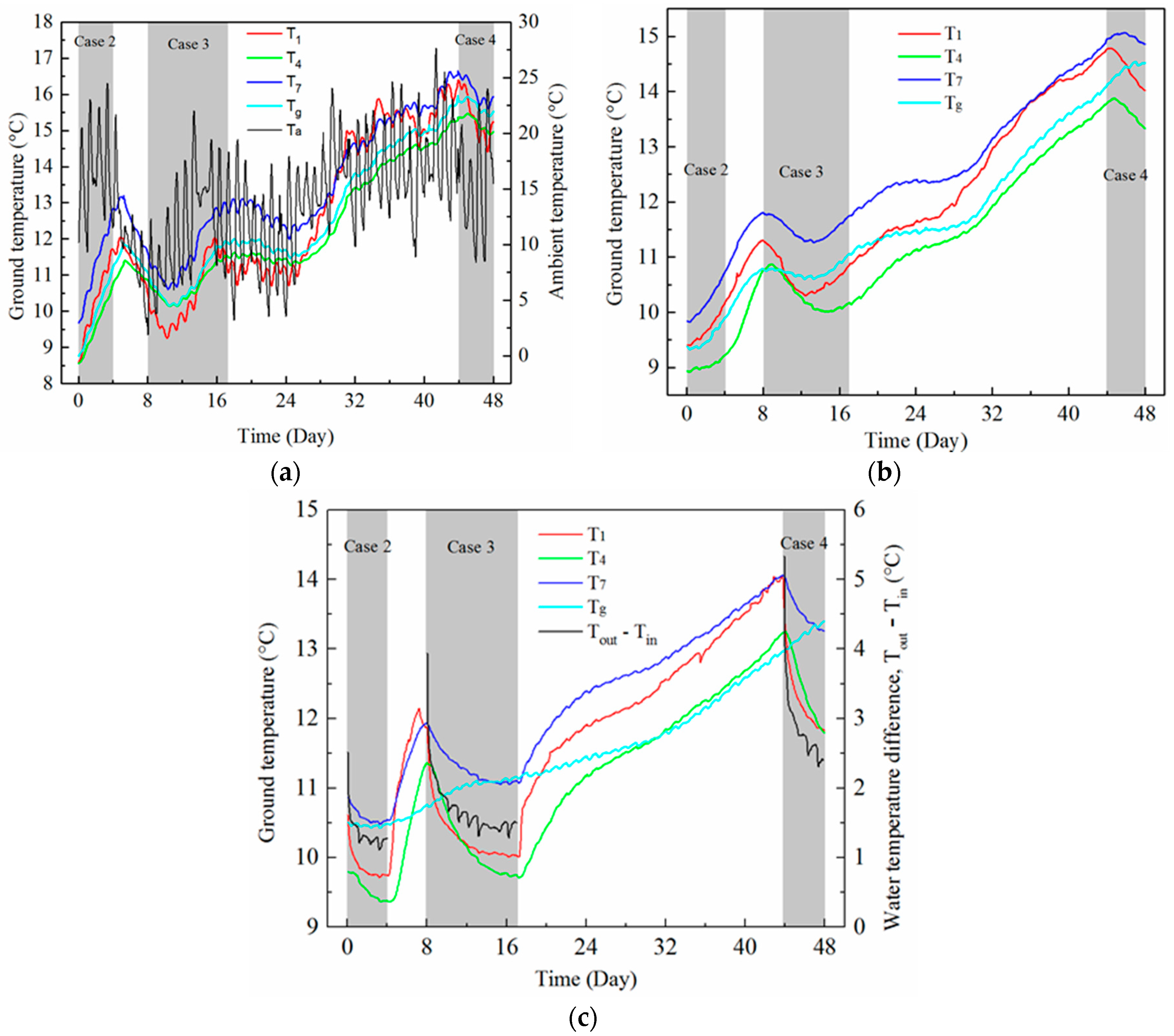
Figure 9.
Time variation of value in different intermittent operations: (a) 6 h and 12 h interval (b) 2 h interval.
Figure 9.
Time variation of value in different intermittent operations: (a) 6 h and 12 h interval (b) 2 h interval.

Figure 10.
Percentage increases in (12 h average) for 12 h and 6 h interval operations based on continuous operation.
Figure 10.
Percentage increases in (12 h average) for 12 h and 6 h interval operations based on continuous operation.

Table 1.
Tube sizing and thermo-physical properties of materials.
| Material | Inner Diameter (mm) | Outer Diameter (mm) | Density (kg/m3) | Specific Heat (J/(kg·K)) | Thermal Conductivity (W/(m·K)) |
|---|---|---|---|---|---|
| Copper (inner) | 14.6 | 15.9 | 8978 | 381 | 387.6 |
| LDPE (outer) | 15.9 | 17.08 | 920 | 3400 | 0.34 |
| Ground: clay [27] | - | - | 1700 | 1800 | 1.2 |
Table 2.
Total maximum uncertainty of measured and calculated parameters.
| Item | Name and Technical Specifications of the Measured Equipment | Uncertainty |
|---|---|---|
| The water temperatures at the inlet and outlet of standing and reclined GHEs | Pt100 Temperature range: −200 to 600 °C Sensor type: Class A, 4 wire | ±0.15 °C |
| Soil temperature in the ground | T-type thermocouple Temperature range: −200 to 200 °C | ±0.5 °C |
| Ambient air temperature | Lutron SD Card Data Logger Model: HT-3007SD Range: 0–50 °C Resolution: 0.1 °C | ±0.8 °C |
| Mass flow rate of water in standing and reclined GHE | TOFCO flow meter Model: FLC-605 Range: 0.5–5 L/min | ±5% |
| Heat exchange rate (W/m) | - | ±5.8% |
| Overall heat transfer coefficient, UA-value (W/°C) | - | ±5.5% |
Table 3.
Experimental conditions in continuous operations.
| Case | Operation Period | Inlet Water Temperature (°C) | Flow Rate (L/min) | Average Initial Ground Temperature around GHE at 1.5 m Depth (°C) | Reynolds Number |
|---|---|---|---|---|---|
| 1 | 23–26 February 2016 | 7 | 2 | 10.4 | 3268 |
| 2 | 4–7 March 2016 | 7 | 1 | 10.4 | 1634 |
| 3 | 12–21 March 2016 | 7 | 1 | 11.3 | 1634 |
| 4 | 17–20 April 2016 | 7 | 1 | 13.7 | 1634 |
Table 4.
Average heat exchange rate and UA-value from 12 to 96 h of operation.
| Operation | Flow Rate (L/min) | Average Heat Exchange Rate (W/m) | Average UA-Value (W/°C) | ||
|---|---|---|---|---|---|
| Standing | Reclined | Standing | Reclined | ||
| Case 1 | 2 | 3.17 | 2.66 | 42.66 | 35.58 |
| Case 2 | 1 | 2.61 | 2.25 | 36.12 | 30.75 |
Table 5.
Calculated value of S.
| Cycle Operation Time | Operation | Period of Integral | S (W·h/(m·°C)) |
|---|---|---|---|
| 120 h | Continuous | Over the whole period | |
| Over every 6 h interval | |||
| Over every 12 h interval | |||
| Intermittent | 6 h interval | ||
| 12 h interval | |||
| 24 h | Continuous | Over the whole period | |
| Over every 2 h interval | |||
| Intermittent | 2 h interval |
© 2017 by the authors. Licensee MDPI, Basel, Switzerland. This article is an open access article distributed under the terms and conditions of the Creative Commons Attribution (CC BY) license (http://creativecommons.org/licenses/by/4.0/).
Share and Cite
MDPI and ACS Style
Ali, M.H.; Kariya, K.; Miyara, A. Performance Analysis of Slinky Horizontal Ground Heat Exchangers for a Ground Source Heat Pump System. Resources 2017, 6, 56. https://doi.org/10.3390/resources6040056
AMA Style
Ali MH, Kariya K, Miyara A. Performance Analysis of Slinky Horizontal Ground Heat Exchangers for a Ground Source Heat Pump System. Resources. 2017; 6(4):56. https://doi.org/10.3390/resources6040056
Chicago/Turabian StyleAli, Md. Hasan, Keishi Kariya, and Akio Miyara. 2017. "Performance Analysis of Slinky Horizontal Ground Heat Exchangers for a Ground Source Heat Pump System" Resources 6, no. 4: 56. https://doi.org/10.3390/resources6040056
Note that from the first issue of 2016, this journal uses article numbers instead of page numbers. See further details here.