
One-Dimensional Renewable Warranty Management within Sustainable Supply Chain


1
Industrial Engineering Department, King Abdulaziz University, Jeddah 22254, Saudi Arabia
2
Department of Mechanical and Industrial Engineering, Northeastern University, Boston, MA 02115, USA
*
Author to whom correspondence should be addressed.
Resources 2017, 6(2), 16; https://doi.org/10.3390/resources6020016
Submission received: 30 December 2016
/
Revised: 21 February 2017
/
Accepted: 25 March 2017
/
Published: 5 April 2017
(This article belongs to the Special Issue Sustainable Supply Chain Management)
Abstract
:Sensor embedded products utilize sensors implanted into products during their production process. Sensors are useful in predicting the best warranty policy and warranty period to offer a customer for remanufactured components and products. The conditions and remaining lives of components and products can be estimated prior to offering a warranty based on the data provided by the sensors. This helps reduce the number of claims during warranty periods, determines the right preventive maintenance (PM) policy, and eliminates unnecessary costs inflicted on the remanufacturer. The renewing, one-dimensional Free Replacement Warranty (FRW), Pro-Rata Warranty (PRW), and combination FRW/PRW policies’ costs for remanufactured products and components were evaluated with/without offering PM for different periods in this paper. To that end, the effect of offering renewable, one-dimensional, Free Replacement Warranty (FRW), or Pro-Rata Warranty (PRW), or combination FRW/PRW warranty policies for each disassembled component and sensor embedded remanufactured product was examined, and the impact of sensor embedded products on warranty costs was assessed. A case study and varying simulation scenarios is examined and presented to illustrate the model’s applicability.
1. Introduction
The increasing tendency in recent years of consumers continually seeking to purchase the latest technology, along with the rapid pace of technological development, has led to diminished product life cycles and an increase in their rate of disposal. Consequently, the Earth’s natural resources and landfill areas are reaching a critical stage. Thus, when technological devices break down or become antiquated, manufacturers often repossess these products to meet or manage regulations. Customers are then also made more aware of the pertinent environmental issues regarding their old equipment.
To meet regulations and reduce landfill use, manufacturers have constructed facilities designed specifically to construct equipment partly from repossessed devices. This process is called the “end-of-life (EOL) product recovery process.” The manufacturers retrieve components, parts, and materials from end-of-life products (EOLPs) through remanufacturing processes, refurbishing, and recycling. The manufacturers obtain an economic benefit from the EOL process.
Disassembly is of primary importance during product recovery because it allows for the extraction of the required materials, subassemblies, and components from the EOL products. A variety of methods can be used to disassemble products, including completing the work on a disassembly line, cell, or single work station. Although disassembly cells and single work stations offer the advantage of being more flexible, disassembly lines produce more and are more efficient for automated operations [1].
With remanufacturing, disposing of EOL products and recycling, the first essential step is to set up the disassembly operation. To deconstruct an EOL product down to its core components, one chooses between destructive, semi-destructive, or non-destructive techniques. The most important goal in disassembling EOL products is to support the recovery process, which is required to minimize the depletion of natural resources during the manufacturing process.
With product recovery, a key question is the uncertainty with producing quality products. The problem stems from the lack of accurate information regarding the condition of the components prior to disassembly. This can be solved by testing each piece of equipment prior to disassembly. However, product disassembly is costly to manufacturers and reduces their profit margins if they are required to devote numerous man-hours to test every used piece of equipment. Additionally, for old components deemed to be useless, this results in a waste of time and expense for the manufacturer attempting to process the EOL devices, resources which could have been better spent elsewhere.
Consumers are hesitant to purchase remanufactured products, questioning their efficacy and reliability. Consequently, they are unsure as to whether the remanufactured products will perform as well as totally new devices. This uncertainty could result in some customers deciding to not purchase the product. Due to this consumer apprehension, remanufacturers often engage in marketing strategies to emphasize the high quality and durability of their products. Often they accomplish this by offering warranties [2].
One means to deal with disassembly yield uncertainty is for manufacturers to engage in the promising use of sensor-embedded products (SEPs). The reason for this is because SEPs utilize sensors implanted during the production process. These sensors monitor the critical components of a product and facilitate data collection. The accumulated data gathered by the sensor can help predict possible future product failures. That is because they estimate the condition of the product component during its EOL stage. Additionally, the information provided by the sensors regarding the missing, replaced, or dysfunctional components prior to disassembly can enable important savings to be had by avoiding wasted efforts in testing, backordering, disposal, disassembly, or holding cost processes [3,4,5].
This gave us the motivation to scrutinize and study the effect of offering non-renewing warranties for products with sensors containing the information within the sensor-embedded remanufactured products. We will quantitatively analyze the expansion achieved by using the SEP’s information in several warranty analyses models depicting a remanufacturing line under various scenarios. Additionally, we will try to minimize costs associated with the warranty and to maximize profits by offering a warranty with an appealing price.
Because the remanufacturing process continually becomes more complex and uncertain, the scope of this paper is limited to the following factors. Required components and EOL products arrive at the remanufacturing facility in accordance with the Poisson distribution. The disassembly and remanufacturing time exponentially assigned to each station are distributed accordingly. Calculating the cost for backorders is based on its duration. Unneeded and unessential EOL products and components are disposed of regularly per a stringent disposal policy. In this study, a pull control mechanism is used in all disassembly line settings, and its use is further reviewed and contemplated. Comparisons of temporal periods and warranty costs are made among the individual warranty policies.
The paper’s primary contribution is that it presents a quantitative assessment of the effect of offering warranties on remanufactured items from a manufacturer’s perspective. Moreover, it proposes an appealing price for the consumers. While there are developmental studies on warranty policies for brand new products and a few on secondhand products, no study evaluates the potential benefits of warranties on remanufactured products in a comprehensive and quantitative manner. In these studies, the improvement in profits obtained by the offering of warranties for differing policies determines the range of how much money can be invested in a warranty, while keeping it profitable overall. This paper studies and scrutinizes the impact of offering renewing warranties on remanufactured products. Specifically, the paper suggests a methodology which simultaneously minimizes the cost incurred by the remanufacturers and maximizes the confidence of the consumers towards buying remanufacturing products. This study uses discrete-event simulation to optimize the implementation of a two-dimensional renewing warranty policy for remanufactured products. The implementation is illustrated using a specific product recovery system called the Advanced Remanufacturing-To-Order (ARTO) system. The experiments used in the study were designed using Taguchi’s Orthogonal Arrays to represent the entire domain of the recovery system so as to observe the system behavior under various experimental conditions. In order to determine the optimum strategy offered by the remanufacturer, various warranty and preventive maintenance scenarios were analyzed using pairwise t-tests along with one-way analysis of variance (ANOVA) and Tukey pairwise comparisons tests for every scenario. This is the first study that evaluates in a quantitative and comprehensive manner the potential benefits of offering one-dimensional renewable warranties with preventive maintenance on remanufactured products.
The rest of the paper is organized as follows: Section 2 describes all the related work from the literature review. System descriptions and renewable one-dimensional warranty are presented in Section 3 and Section 4, respectively. Section 5 presents the design-of-experiment study. Assumptions and notations are given in Section 6. Section 7 addresses the preventive maintenance analysis. The failure analysis and warranty formulation are included in Section 8 and Section 9, respectively. Finally, results and conclusions are given in Section 10 and Section 11, respectively.
2. Literature Review
2.1. Environmentally Conscious Manufacturing and End-of-Life Product Recovery
In recent years, the number of studies dealing with environmentally conscious manufacturing and product recovery (ECMPRO) issues have gained gratuitous attention from researchers [4,6]. This is partially due to environmental factors, government regulations, and public demands, but on the other side, it is also due to economical profits obtained by implementing reverse logistics and product recycling resolutions. Manufacturers respond to consumer awareness of environmental issues and stricter environmental legislations by establishing designated facilities designed for the purpose of minimizing waste amassment by recovering materials and components derived from EOL products [1]. Researchers have shed light on the panoptic environmentally conscious dilemmas involved in product manufacturing. As a result, researchers have released reviews of these panoptic issues involved in environmentally conscious manufacturing and product recovery (see for example, [7,8,9]). Disassembly is the most apex in the remanufacturing research area, which is due to its significant role in the recovery system. For different aspects involved in disassembly, view the book by Lambert and Gupta [10].
Many researchers have studied remanufacturing processes because traditional production planning methods have fallen short in regards to the recovery of products. A review of 76 journal articles on the remanufacturing processes was reported by Lage and Godinho-Filho [11]. Morgan and Gagnon [12] organized and reviewed journals up to 2011 with the intention of gathering a progression timeline of remanufacturing. The impact of two-product joint life cycles on the capacity planning of remanufacturing networks was presented by Georgiadis and Athanasiou [13]. The authors put emphasis on the inherent uncertainties of remanufacturing systems and proposed a system dynamics model design representing capacity-planning experiments. Another study by the same authors dealt with long-term demand-driven capacity planning policies in the reverse channel of closed-loop supply chains with remanufacturing under high capacity acquisition cost. This was coupled with uncertainty in actual demand, sales patterns, quality, and timing of end-of-use product returns. The authors studied the system’s response in terms of transient flows, actual and/or desired capacity level, capacity expansions/contractions, and total supply chain profit by employing a simulation-based system dynamics optimization approach [14]. For additional aspects of remanufacturing, note the book by Ilgin and Gupta [15].
2.2. Sensor Embedded Products
Manufacturers are now able to build sensors in smaller sizes and at lower costs due to the expansion of technology. The use of sensor-based technologies on after-sale product condition monitoring is an active research area. Starting with the study of Scheidt and Shuqiang [16], different methods of data acquisition from products during product usage were presented by the researchers [17,18,19]. Cheng et al. [20] developed a generic embedded device that could be installed in different types of equipment, including manufacturing equipment, portal servers, and automated, guided vehicles. This device has the ability of retrieving, collecting, and managing equipment data with the help of an embedded real-time operating system and several software modules. Yang et al. [21] and Yang et al. [22] developed an intelligent product model for discovering product service systems for consumer products, such as fridge/freezer appliances and game consoles for PlayStation 2. In this model, an intelligent data unit was installed in each product to acquire data during usage and the distribution stages of its life cycle. The procurement of the essential life-cycle components of a product with sensors embedded in it is presented by Zeid et al. [23] and Vadde et al. [24]. Additional studies aim to further explore whether or not the use of embedded sensors increases product life-cycle management effectiveness. A comprehensive survey on the commercial sensor systems used in health management for electronic products and systems was reported by Pecht [25]. Fang et al. [26] investigated the modern practices leading toward the eventual development of embedded sensors in products in two primary categories (viz., embedding sensors in products and representing and interpreting sensor data).
Another avenue of research hinges on the life cycle data analysis obtained via the implementation of various sensor-based data acquisition methods. In this scope, Mazhar et al. [27] presented an integrated, two-stage approach which combined the Weibull analysis and multiple linear regression to assess the component reliability in refurbished products based on their life cycle data. Mazhar et al. [28] carried out a similar analysis by integrating Weibull analysis with neural networks. Herzog et al. [29] compared the performance of several neural network variations in the prediction of the residual life of machines and components.
Although the majority of the studies presented above focus on the development of SEP models that enable product data acquisition during their life cycle and/or in their EOL phase, only a select few number of researchers have conferred a cost-benefit analysis. Klausner et al. [30] analyzed the trade-off between the higher initial manufacturing costs caused by using an electronic data log (EDL) in products and the cost savings from the reuse of used motors. Simon et al. [31] improved the cost-benefit analysis of Klausner et al. [32] by taking into consideration the limited lifespan of a product’s design. It was revealed that under certain circumstances, product servicing offers more readily reusable components in contrast to EOL recovery of parts.
The use of Radio-Frequency Identification (RFID) tags have been studied by Kiritsis et al. [33] and Parlikad and McFarlane [34] to offer effortless access for the retrieval, updating, and management of information involved in the product life cycle. The effect of using RFID in ameliorating the quality uncertainty associated with remanufacturing processes has been examined by Kulkarni et al. [35], who made use of an application of RFIDs where active RFIDs were used for easy identification and localization of components within a remanufacturing facility, while passive RFIDs, on the other hand, were permanently tagged onto components of remanufacturable products at the beginning of their service life, which was reported by Ferrer et al. [36].
2.3. Warranty Analysis
A warranty is a contractual obligation incurred by a manufacturer (vendor/seller) in connection with the sale of a product. The purpose of a warranty is to establish liability in the rare event that a purchased item fails prematurely or is unable to perform its intended function. These contracts specify the promised product performance and when this expected performance level is not met, a return of compensation is available to the buyer as compensation [37,38]. Product warranties have different main functions. One of the functions is insurance and protection, permitting buyers to transfer the risk of product failure back to the sellers [39]. Secondly, product warranties can also signal product reliability to customers [40,41,42,43], and lastly, the sellers can use warranties to extract additional profitability [44].
In contrast with massive literature on warranty policies for new items, up to now study on warranty policies for second-hand items has received less attention. Modelling the warranty cost analysis for used products is a novel field of research with a limited number of publications. The optimal upgrade strategies for second-hand items under both the virtual age along with the screening test reliability development methods are presented by Saidi-Mehrabad et al. [45] and Shafiee et al. [46], who built a stochastic model designed to examine the optimal degree of investments for increasing the reliability of secondhand products under free repair warranty (FRW) policies. They concluded that a larger number of investments meant larger declines in the virtual age and greater reliability levels of the upgraded product. A stochastic reliability improvement model for used products with warranties and Cobb-Douglas-Type production function to reach the optimal upgrade level was presented by Shafiee et al. [47]. A study to determine the optimal upgrade, selling price, and maximum expected profit with restrictive assumptions about the age distribution was conducted by Naini and Shafiee [48]. They built a mathematical model to implement a parametric analysis on the items’ chronological ages to detect and determine the best policies. Yazdian et al. [49] adopted an integrated mathematical model that was not reliant on the specific age of the received item in order to determine the typically experienced remanufacturer decisions. The warranty policy and its effect on consumer behavior from the perspective of consumers has been studied by Liao et al. [50]. A novel mathematical–statistical model was proposed where decisions involving the pricing of returned used products (cores), with the degree of their remanufacturing, selling price, and warranty period for the final remanufactured products was used to investigate the joint optimization of remanufacturing, pricing, and warranty decision-making for end-of-life products [51]. Kuik et al. [52] presented mathematical models to examine two types of the proposed extended warranty policies for manufacturers so that they could make comparisons of their possible gained profits of remanufactured products by the manufacturers who supplied them. In contrast, the analysis of warranty costs for remanufactured products has not yet received any significant attention. However, there are few papers that consider the warranty for the remanufactured products’ reverse and closed-loop supply chain management. Base and extended one-dimensional warranty can be offered for remanufacturing products using Free Replacement Warranty (FRW) and Pro-Rata Warranty (PRW) policies [52,53,54]. Also, renewable, nonrenewable, one- and two-dimensional warranty policies can be offered for EOL-derived products [55,56,57,58,59].
2.4. Maintenance Analysis
Maintenance has a significant role in product reliability and quality. In the literature, maintenance is classified into two main types, viz., corrective maintenance (CM) and preventive maintenance (PM). CM occurs when an item fails, and it is performed to restore a failure item to an operational state; PM is performed before an item fails in order to reduce degeneration and failure rate. In the case of products with short remaining life, the warranty is also comparatively short and only CM actions are offered, whereas in a product with long remaining life, the warranty could be relatively long and warranty servicing costs can be reduced by carrying out PM actions. Thus, there is a relation between warranties and CM and PM.
The literature on maintenance policies is extensive. Several review papers on maintenance policies have appeared [60,61,62]. We refer the reader to a book by Nakagawa [63] for the detailed information on the general area of maintenance theory. An extensive review of modelling maintenance policies can be found in a book by Nakagawa [64].
Maintenance policies for second-hand products during the warranty period was not receiving researchers’ interests [65]. Yeh et al. [66] proposed two periodical age reduction PM models to decrease the high failure rate of the second-hand products. Kim et al. [67] studied the optimal periodic PM policies of a second-hand item following the expiration of warranty. From the manufacturer perspective, it is meaningful to carry out PM actions only when the saving of warranty servicing costs exceeds the additional costs that occur by performing PM activities. Therefore, developing PM policies for second-hand products still needs further research studies.
3. System Description
The Advanced Remanufacturing-To-Order (ARTO) system deliberated on in this study is a sort of product recovery system. A sensor embedded air conditioner (AC) is considered here as a product example. Based on the condition of EOL AC, it goes through a series of recovery operations, as shown in Figure 1. Refurbishing and repairing processes may require reusable components in order to meet the demand of the product. This requirement satisfies both the internal and the external component demands. Thus, both will be satisfied using disassembly of recovered components. There are three different types of item arrivals in the ARTO system: either EOL products for recovery processes, failed SEPs needing to be rectified, or SEPs due for maintenance activities.
First, EOL ACs arrive at the ARTO system for information retrieval using a radio frequency data reader that is stored in the facility’s database. Then the ACs go through a six-station disassembly line. Complete disassembly is performed for the purpose of extracting every single component. Table 1 represents the precedence of relationships between the AC components. There are nine components in an AC: the evaporator, control box, blower, air guide, motor, condenser, fan, protector, and compressor. Exponential distributions are used to generate the station disassembly times, interarrival times of each component’s demand, and interarrival times of the EOL AC. Exponential distributions are used to generate the disassembly times at each station, interarrival times of each component’s demand, and interarrival times of the EOL AC (The exponential distribution fits the events cited above because it is the only distribution with the “lack-of-memory” property. After waiting a minute without a SEPs arrival, the probability of a product arriving in the next two minutes is the same as was the probability (a minute ago) of getting a product in the following two minutes. As you continue to wait, the chance of something happening “soon” neither increases nor decreases [68]). After retrieval of the information, all EOLPs are shipped either to station 1 for disassembly or, if an EOLP only needs a repair for a specific component, it is instead sent to its corresponding station. Two different types of disassembly operations, viz., destructive or nondestructive, are used depending on the component’s condition. If the disassembled component is not functional (broken, zero percent of remaining life), then destructive disassembly is utilized in such a way that the other components’ functionality is not damaged. Therefore, unit disassembly cost for a functional component is higher than for a nonfunctional component. After disassembly, there is no need for component testing due to the availability of information regarding components’ conditions from their sensors. It is assumed that the demands and life cycle information for EOLPs are known. It is also assumed that the retrieval of information from sensors costs less than the actual inspecting and testing.
Recovery operations differ for each SEP based on their overall condition and estimated remaining life. Recovered components are used to meet spare parts demands, while recovered or refurbished products are used for consumer product demands. Also, material demands are met using recycled products and components. Recovered products and components are characterized based on their remaining lifespans and are placed in different life-bins (e.g., one year, two years, etc.) where they wait to be retrieved via a customer demand. Underutilization of any product or component can happen when it is qualified for a higher life-bin but is placed in a lower life-bin because the higher life-bin is full. Any product, component, or material inventory that is greater than the maximum inventory allowed is assumed to be of excess and is instead used for material demand or is simply disposed of.
EOLPs may have missing or nonfunctional (broken, zero remaining life) components that need to be replaced or replenished during the repairing or refurbishing process in order to meet certain remaining life requirements. EOLPs may also consist of components having lesser remaining lives than desired, and, for that reason, might also have to be replaced. A further case of failure of SEPs during the warranty period, the failed ACs arrive at the ARTO system for information retrieval using a radio frequency data reader that is stored in the facility’s database. Then the failed ACs go through the recovery operations as explained before the same as an EOLP.
Finally, in order to reduce the risk of failure, PM actions are carried out during the warranty period. Here, if the remaining life of a remanufactured AC reaches a pre-specified value, the remanufactured SEPs arrive at the ARTO system for information retrieval using a radio frequency data reader that is stored in the facility’s database. Then, the SEPs go through four maintenance activities based on the information from the sensor about their condition. These maintenance activities include measurements, adjustments, parts replacement, and cleaning. When PM actions are performed with degree δ, the remaining life of the remanufactured ACs will be δ units of time more than before, as shown in Figure 2. Meanwhile, any failures between two successive PM actions during the warranty period are rectified at no cost to the customer.
4. Renewable One-Dimensional Warranty
During the process of deciding to purchase a product, the buyer usually compare features of a product with other competing brands that are selling the same product. In some cases, the competing brands produce similar products bearing similar features such as the costs, special characteristics, quality, credibility of the product, and even insurance from the provider. In these cases, after sale factors come into effect, such as the discount, warranty, availability of parts, repairs, and other services. These factors will be very significant to the buyer in such a situation; so will the warranty, since it further assures the buyer of the reliability of the product.
A warranty is an agreement that requires the manufacturer to correct any product failures or to compensate the buyer for any problems that may occur with the product during the warranty period in relevance to its sale. The objective of the warranty is to promote the product’s quality and guarantee its performance in order to assure productivity for both the manufacturer and the buyer. For a given product, the warranty cost (in a statistical sense) is the same for all new items if the manufacturer has good quality control. In contrast, each EOL product is different due to factors such as age, usage, and maintenance history. This makes the warranty cost for each remanufactured product derived from an EOL item statistically different.
The importance of warranties for remanufactured products is increasing because consumers are becoming more demanding of product quality and the increase in customer’s awareness of the environment will increase the demand for remanufactured products and future costs of replacement/repair in case of product failures. Therefore, warranty management has become very important to remanufacturers of remanufactured products. They need to estimate the warranty cost in order to factor it into the pricing structure. Failure to do so can result in the remanufacturers incurring loss, as opposed to profit, with the sale of remanufactured items. Analyses of warranty costs for remanufactured products are more complex when compared to new products because of the uncertainties in usage and maintenance history. Moreover, warranty policies similar to new and secondhand products may not be economically acceptable from the remanufacturer’s point of view. Therefore, there is a need to test and compare these warranty policies for remanufactured products and estimate the expected warranty cost associated with these policies. There are other related issues such as the servicing strategies involving remanufactured spare parts in the replacement/repair of failures during the warranty period.
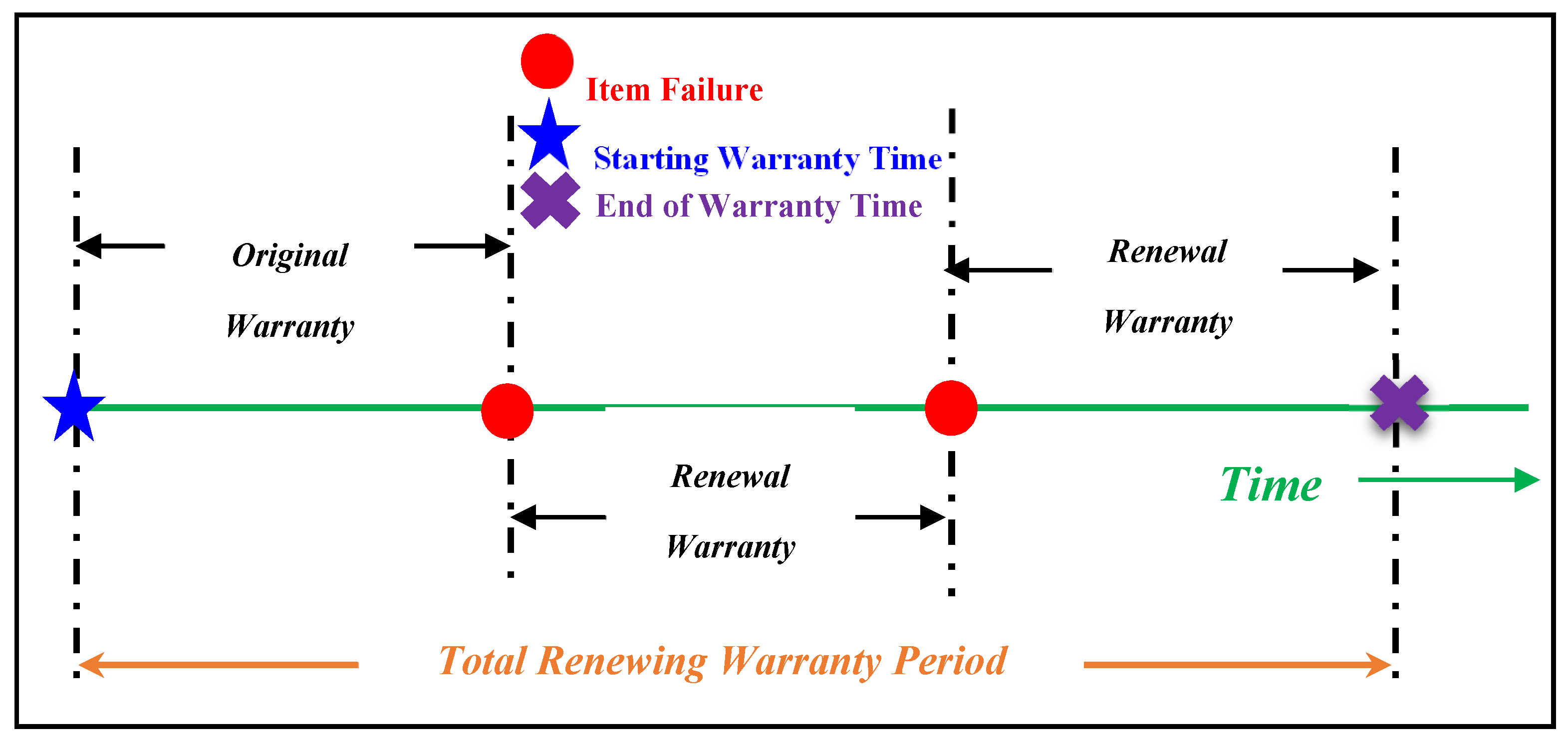
In the one-dimensional warranty, a policy is defined by an interval called the “warranty period”, W, which is defined with respect to a signal variable, such as age or amount of usage. For renewing policies, the warranty period begins anew with each replacement or repair. Therefore, the warranty period is uncertain, as the warranty ceases only when an item does not fail for a period W, as shown in Figure 3. There are many different available one-dimensional consumer warranty policies which most products are sold with. The most famous renewing consumer warranties are the Renewing Free Replacement Warranty (FRW) and Renewing Pro-Rata Warranty (PRW), or a combination of both FRW/PRW.
Under the FRW policy, the manufacturer agrees to either repair or provide a replacement free of charge up to a time W from the initial purchase. Whenever there is a malfunction, the failed item is replaced by a new one with a new warranty whose terms are identical to the original.
5. Design-of-Experiments Study
According to a comprehensive study for the quantitative evaluation of the SEPs on the performance of a disassembly line conducted by Ilgin and Gupta [69], it was shown that smart SEPs are a favorable resolution in handling remanufacturing customer uncertainty. To test this claim on ARTO, we built a simulation model to represent the full recovery system and observed its behavior under different experimental conditions. ARENA program, Version 14.5, was used to build the discrete-event simulation models. A three-level factorial design was used with 51 factors that were each considered at three levels. These were identified as low, intermediate, or high levels. The reason that the three-level designs were proposed was to model possible curvature in the response function and to handle the case of nominal factors occurring at three levels. The parameters, factors, and factor levels are given in Table 2 and Table 3. A full-factorial design with 54 factors at three levels requires an extensive number of experiments (viz., 5.815 × 1025). To reduce the number of experiments to a practical level, a small set of all the possible combinations was picked. The selection method of an experiment’s number is called a partial fraction experiment, which yields the most information possible of all the factors that affect the performance parameter with the minimum number of experiments possible. For these types of experiments, Taguchi [70] enacted specific guidelines. A new method of conducting the experimental design was to use a special set of arrays called orthogonal arrays (OAs) that were built by Taguchi. Orthogonal arrays provided a way to only have to conduct a minimal number of experiments. In most cases, the use of an orthogonal array is more efficient when compared to many other statistical designs. The minimum number of experiments that are required to conduct the Taguchi method can be calculated based on the degrees of freedom approach.
So, the number of experiments must be greater than or equal to a system’s degrees-of-freedom. Precisely, L109(354) (i.e., 109 = [(Number of levels − 1) × Number of Factors] + 1) Orthogonal Arrays were chosen because the degree of freedom ARTO system is 101, meaning it requires 101 experiments to accommodate 54 factors upon three different levels. Additionally, an orthogonal array assumes that there is no interaction between any two factors.
Furthermore, for validation and verification purposes, animations of the simulation models were built along with multiple dynamic and counters plots. Two thousand replications with six months (eight hours a shift, one shift a day, and five days a week) were used to run each experiment. Arena models calculate the profit using the following equation:
where SR is the total revenue generated by the product, component, and material sales during the simulated run time; CR is the total revenue generated by the collection of EOL ACs during the simulated run time; SCR is the total revenue generated by selling scrap components during the simulated run time; HC is the total holding cost of products, components, material, and EOL ACs during the simulated run time; BC is the total backorder cost of products, components, and material during the simulated run time; DC is the total disassembly cost during the simulated run time; DPC is the total disposal cost of components, material, and EOL ACs during the simulated run time; TC is the total testing cost during the simulated run time; RMC is the total remanufacturing cost of products during the simulated run time; TPC is the total transportation cost during the simulated run time; PMC is the total preventive maintenance cost during the simulated run time and WC is the total warranty cost.
Profit = SR + CR + SCR − HC − BC − DC − DPC − TC − RMC − TPC − PMC − WC
In each EOL AC, there are three types of scraps that need to be recovered and sold. The evaporator and condenser are sold as copper scrap, chassis and metal covers are sold as steel scraps, and blowers, fans, and air guides are sold as fiberglass. All the other components are considered to be waste components. Scrap revenue from steel, copper, and fiberglass components is calculated by multiplying their weight in pounds by the units of scrap revenue produced by each metal type. Disposal cost is calculated as well by multiplying the waste weight by the unit disposal cost. The time of retrieving information from smart sensors is assumed to be 20 s per AC. The transportation cost is assumed to be $50 for each trip taken by the truck. There are different prices in the secondary market of recovery product due to different level of quality.
6. Assumptions and Notations
This section starts with the model assumptions. Then, the notation of all the parameters used in this paper.
6.1. Assumptions
The following assumptions has been considered to simplify the analysis:
- The failures are statistically independent.
- Every item failure under warranty period results in a claim.
- All claims are valid.
- The failure of a remanufactured item is only a function of its age.
- The time to carry out the replacement/repair action is relatively small compared to the mean time between failures.
- The cost to service warranty claim (for repair/replacement of failed components) is a random variable.
6.2. Notations
| W | Warranty period |
| W1 | Sub-interval of warranty period |
| Cs | Operating cost of item |
| Cp | Sale price of item |
| S(y) | Refund function |
| n | Number of components in an item |
| m | Level of PM effort |
| RL | Remaining life of item at sale |
| RLi | Remaining life of component i (1 ≤ i ≤ n) |
| Virtual remaining life after performing PM activity | |
| Remaining life increment factor of PM with effort m | |
| (1 − p) | Probability that a new component is needed in the replacement. |
| Ui, Li | Upper and Lower range of replacement component’s remaining life |
| k | Number of free replacements required under renewing FRW |
| Λi | Intensity function of non-stationary Poisson process |
| Miu | Renewal function associated with Fiu(x) |
| E[.] | Expected value of expression within [.] |
| Fi(x) | Failure distribution of a remanufactured component i |
| Fiu(x) | Distribution function for times to failure of remanufactured component used in replacement |
| H(rl) | Distribution function for RL when remaining life is unknown |
| Hi(rl) | Distribution function for RLi (for replacement components) |
| N(W; RL) | Number of failures over the warranty period with remaining life, RL |
| Λ(RL) | Intensity function for system failure |
| Fw(y) | Distribution function for the first failure in the period [W1, W) given by the excess remaining life of renewal process associated with failures in the period [0, W1) |
| Y | Excess remaining life of renewal process associated with failures in the period [0, W1) |
| Cd(W1; RL) | Warranty cost to the remanufacturer in the period [0, W1) for an item of remaining life RL |
| Cb(W1, W; RL) | Cost to the buyer for an item of remaining life RL |
| Cd(W1, W; RL) | Total warranty cost to the remanufacturer for item of remaining life RL |
| Cd(W1, W) | Total warranty cost to the remanufacturer for item of remaining life RL unknown |
7. Preventive Maintenance Analysis
Usually, PM activities involve a set of maintenance tasks, such as, cleaning, systematic inspection, lubricating, adjusting and calibrating, replacing different components, etc. [71]. The right PM activities can potentially represent an efficient way to reduce the number of failures, and as a result, reduce the warranty cost and increase customer satisfaction. This study adopts the modelling framework proposed by Kim et al. [72] to model the effect of PM activities.
A series of PM activities of a remanufactured item are performed at remaining life rl1, rl2, …, rlj, …, with rl0 = 0. Here, the effect of PM results in a restoration of the item so that the item’s virtual remaining life is effectively increased. The concept of virtual age is introduced in [73], and then extended in [74]. In this study, the jth PM only reimburses the damage accrued during the time between the (j − 1)th and the jth PM activities, as a result an arithmetic reduction of virtual remaining life can be obtained [75]. Therefore, the virtual remaining life after performing the jth PM activity (i.e., rlj,) is then given by
where m is the level of PM effort, and δ(m), m = 0, 1, …, M, is the remaining life increment factor of PM with effort m. Note that the effect of PM depends on its level m, 0 ≤ m ≤ M, and its relationship with the remaining life is characterized by the age-incremental factor δ(m). Larger values of m represent greater PM effort, hence δ(m) is an increasing function of m with δ(0) = 0 and δ(M) = 1. More specifically, if m = 0, then vj = RLj, j ≥ 1, which means that the item is restored to as bad as old (ABAO); if m = M, the item is restored back to as good as new (AGAN); while in a more general case m ∈ (0, M), the item is partially restored (i.e., the PM activity is imperfect).
8. Failures Analysis
Most products are complex and have multiple parts, so that an item can be viewed as a system consisting of several components. The failure of an item occurs due to the failure of one or more components. A remanufactured product or component is categorized in terms of two states, viz., working or failed. The time intervals between consecutive failures are random variables and modelled by proper distribution functions. Interchangeably, the number of failures over time can be modelled by a suitable counting process.
The actions to make a failed item operational depend on whether the failed component(s) are repairable or not. In the case of a repairable component, the remanufacturer has the option of repairing or replacing it by a remanufactured working component, if available. If not, a new component will be used to rectify the claim. In case of repairable components, the characterization of subsequent failures depends on the type of repair (e.g., minimal repair, imperfect repair, and so on). Similarly, in the case of a non-repairable component, the remanufacturer can use a remanufactured working component in the replacement to make the item operational.
Time to first failure of a remanufactured component depends on the mean remaining lifetime (MRL) and the PM of the component at the time of sale of the remanufactured product. If the sensor information about an EOL component indicates that it has never failed, or was always minimally repaired, then the remaining life of the component at sale is the same as that of the item. Usually, the MRL of a remanufactured component at sale differs due to the replacement or repair and maintenance actions. Therefore, the time to first failure under warranty needs to be defined. Let RLi denote the remaining life of remanufactured component, i. There are two cases: either RLi is known because of embedded sensor or RLi is unknown because it is a conventional product.
The sensor embedded in the item provides the remanufacturer with the MRL of the item at sale and the virtual remaining life due to upgrades and maintenance information. The item failure is modelled by a point process with intensity function Ʌ(RL), where RL represents the remaining life of the item. Ʌ(RL) is an increasing function of RL, indicating that the number of failures increases with remaining life. The failures over the warranty period [RL, RL + W) occur according to a non-stationary Poisson process with intensity function Ʌ(RL). This implies that N(W; RL), the number of failures over the warranty period W for an item of remaining life RL at the time of sale and virtual remaining life v, is a random variable with
The expected number of failures over the warranty period is given by
9. Warranty Formulation
In this model, the component’s actual remaining life, RLi, and virtual remaining life, vi, are known using embedded sensors, and components which fail during the warranty period will be replaced by remanufactured components. The remaining life of remanufactured components used in the replacement varies and can range from Li to Ui according to a distribution function Hi(rl). As a result, the failure distribution of a remanufactured component is given by:
When a remanufactured component is not available, one needs to use a new component. Let (1 − p) denote the probability that a new component is needed in the replacement.
Since an embedded sensor is used to determine the remaining life of the component, the distribution for the first failure, Fi1(x) is given by:
In the meantime, distribution for succeeding failures, Fi2(x), is given by:
where Fiu(x) is given by:
The number of failures during warranty period Ni (W; RLi) is given by:
and for the succeeding failures given by:
Accordingly, the expected number of failures over the warranty period is given by:
where Mi2(x) is the renewal function associated with Fi2(x) given by:
Fi1(x) is given by:
9.1. Analysis of Renewing Free Replacement Warranty Policy
This section carries out an analysis of the Renewing Free Replacement Warranty (FRW) Policy to determine the expected warranty costs.
Under this policy, the remanufacturer resolves all failures in the interval [0, W1) at no cost to the buyer. The warranty period after replacement/repair is the remaining period of the original warranty. If a failure occurs in the interval [W1, W) then the item is replaced/repaired by the remanufacturer at no cost to the buyer and returned with a new warranty of duration (W − W1). Let K be the number of free replacements required under renewing FRW. Then Xk+l is the first item lifetime in the sequence of replacements that is at least of length (W − W1). K is a random variable with
The expected number of renewals beyond W1 is given by:
where Fiu(W − W1) = l − Fiu(W − W1).
As a result, the expected warranty cost to the remanufacturer E[Cd(W1, W; RL)] is given by:
9.2. Analysis of Renewing Pro-Rata Warranty Policy
This section carries out an analysis of the Renewing Pro-Rata Warranty (PRW) Policy to determine expected warranty costs.
Under this policy, the remanufacturer supplies a replacement item at a reduced price if an item fails before the warranty period W. This can be viewed as a conditional refund since the buyer is constrained to use the refund to buy a replacement item. The amount refunded is a function of the time period (X) elapsed subsequent to the sale. The replacement item comes with a new warranty identical to the original one.
This paper considered a linear refund function S(Y) given by:
Let K be the number of renewals under renewing PRW. K is a random variable with
The expected number of replacements is given by:
Then, the expected warranty cost to the remanufacturer, E[Cd(W)], is given by:
9.3. Analysis of FRW-PRW Combination Policy
This section carries out an analysis of Renewing FRW-PRW Policy to determine expected warranty costs.
Under this policy, the remanufacturer replaces failed items at no cost to the buyer up to W1 (W1 < W). If a failure occurs in the interval [W1, W) the remanufacturer refunds a fraction of the sale price and the warranty terminates.
Since the item has a sensor embedded in it to retrieve all the data needed, the remaining life RL can be estimated. The failures over [0, W1) are given by a modified renewal process. In this case, the first failure is given by Equation (5) and subsequent failures are given by Equation (11). The expected number of failures in [0, W1) is given by Equation (12).
Therefore, the expected warranty cost to the remanufacturer for failures in [0, W1), E[Cd(W1; RL)], is given by:
where Miu(x) is the renewal function associated with Fiu(x) and cp is the processing cost per item to the remanufacturer. For failures over the interval [W1, W) we need the excess remaining life, Y, when the warranty term changes from FRW to PRW. This is given by FW(y) as follow:
Let S(Y) denote the linear refund function, which is given by Equation (18) where Cs(RL) is the sale price. Then the expected warranty cost to the remanufacturer resulting from a failure in [W1, W) is given by:
Combining the costs over the two intervals, it will result in the following:
10. Results
The results are divided into three sections. Section 10.1 deals with the evaluation of the effect of offering different warranty policies to help the decision maker choose the best warranty policy to offer. Section 10.2, shows a quantitative assessment of offering PM on warranty policies. Finally, Section 10.3 presents a quantitative assessment of the impact of SEPs on the warranty and maintenance costs and policies to the remanufacturer.
10.1. Remanufacturing Warranty Policies Evaluation
In this section, the results to compute the expected number of failures and expected cost to the remanufacturer were obtained using the ARENA 14.5 program. We evaluate different warranty periods with and without offering a preventive maintenance policy during each period.
10.1.1. Renewable Free Replacement Warranty (FRW) Policy
Table 4 presents the expected number of failures and cost for remanufactured ACs and components for renewable FRW, PRW, and Combination Policies. In Table 4, the expected number of failures represents the expected number of failed items per unit of sale. In other words, it is the average number of free replacements that the remanufacturer would have to provide during the warranty period per unit sold. Expected cost to the remanufacturer includes the cost of supplying the original item, Cs. Thus, the expected cost of warranty is calculated by subtracting Cs from the expected cost to remanufacturer. For example, from Table 4, for W = 0.5 and RL = 1, the warranty cost for an AC is $39.88 − Cs =|$39.88 − $55.00| = $15.12 which is ([$15.12/$55.00] × 100) = 27.49% saving of the cost of supplying the item, Cs, which is significantly less than $55.00, Cs. This saving might be acceptable, but the corresponding values for longer warranties are much lower. For example, for W = 2 years and RL = 1, the corresponding percentage is ([|$48.90 − $55.00|/$55.00] × 100) = 11.09%.
10.1.2. Renewable Pro-Rata Warranty (PRW) Policy
The results for PRW are also given in Table 4. Here too, the expected cost of providing a warranty can be calculated as above. For example, the cost of a warranty for 3 years remaining life AC with W = 2 years will cost $76.60 − Cs = $76.60 − $55.00 = $21.60, which is 39.27% of the cost of supplying the item, Cs.
10.1.3. Combination Free Replacement Warranty (FRW) Policy
Here too, the results are given in Table 4 and the expected cost of providing a warranty can be calculated in a similar manner as above. For example, the cost of warranty for 3 years remaining life AC with W = 2.0 years will cost |$31.44 − $55.00| = $23.56, which is 42.84% of the cost of supplying the item, Cs.
10.2. Preventive Maintenance Evaluation
In order to assess the impact of PM on warranty cost, pairwise t tests were carried out for each performance measure. Table 5 presents the ninety-five percent confidence interval, t value, and p value for each test. According to Table 5, PM achieves statistically significant savings in holding, backorder, disassembly, disposal, remanufacturing, transportation, warranty, PM costs, and number of warranty claims. In addition, SEPs provide statistically significant improvements in total revenue and profit. According to Table 6, the lowest average value of warranty, PM costs, and the number of warranty claims during the warranty period for remanufactured ACs across all policies are $6390.68, $1225.79, and 8483 claims, respectively, for the Sensor Embedded Model with FRW warranty policy, whereas the conventional AC has the worst values for the warranty, PM costs, and the number of warranty claims during the warranty period.
10.3. Sensor Embedded Evaluation
10.3.1. Effect of SEPs on Warranty Cost
According to Table 7, the lowest average value of warranty costs and the number of warranty claims during the warranty period for remanufactured conventional ACs across all policies are $8733.10 and 11,497 claims, respectively, for the combination FRW/PRW warranty policy.
10.3.2. Effect of SEPs on Warranty Policies
The MINITAB-17 program was used to carry out one-way analyses of variance (ANOVA) and Tukey pairwise comparisons for all the results in this section. ANOVA was used in order to determine whether there are any significant differences between the warranty costs, number of claims, and PM costs for the four different models, viz., the conventional model, SEPs with FRW, SEPs with PRW, and SEPs with FRW/PRW, while the Tukey pairwise comparisons were conducted to identify which models are similar and which models are not. Table 8 shows that there is a significant difference in warranty costs between different warranty policies. Tukey test shows that all the models are different and that the SEP model with FRW policy has the lowest warranty cost. In addition, there is a significant difference in the number of warranty claims between different warranty policies (see Table 9). Here, Tukey test shows that there is no difference between SEP Model with FRW/PRW policy and SEP Model with PRW policy in the number of claims, while the conventional model and SEP model with FRW are different. The FRW policy has the lowest number of claims. Finally, Table 10 shows that there is a significant difference in PM costs between different warranty policies. Tukey test shows that all models are different and that the SEP model with FRW policy has the lowest costs. These results can be useful in the determining the economical warranty policy associated with embedding sensors in ACs.
As a result, it is found that anticipated warranty costs and maintenance are essential pieces of information upon which remanufacturers base pricing and maintenance action decisions.
11. Conclusions
This study used discrete-event simulation to optimize the implementation of a two-dimensional renewing warranty policy for remanufactured products. The implementation was illustrated using a specific product recovery system called the Advanced Remanufacturing-To-Order (ARTO) system. The experiments used in the study were designed using Taguchi’s Orthogonal Arrays to represent the entire domain of the recovery system so as to observe the system behavior under various experimental conditions. In order to determine the optimum strategy offered by the remanufacturer, various warranty and preventive maintenance scenarios were analyzed using pairwise t-tests along with one-way analysis of variance (ANOVA) and Tukey pairwise comparisons tests for every scenario.
This paper results in the formulation and presentation of three different one-dimensional renewable warranty policies, including related maintenance actions, for sensor-embedded remanufactured products, in addition to mathematical and stimulation modeling and analysis for the anticipated costs for these policies. The proposed methodology is able to simultaneously minimize the cost incurred by the remanufacturer, optimize the warranty price and period, and optimize the preventive maintenance strategy resulting in increased consumer confidence. This is the first study that evaluates in a quantitative and comprehensive manner the potential benefits of offering one-dimensional renewable warranties with preventive maintenance on remanufactured products.
Acknowledgments
The authors would like to thank the reviewers for their highly constructive comments and suggestions in improving this article.
Author Contributions
A.Y.A. reviewed the literature on environmentally conscious manufacturing and product recovery, disassembly to order systems, sensor embedded technology, warranty and maintenance used, and developed the simulation models. He carried out the warranty, maintenance analysis, and orthogonal arrays-based statistical experiments. S.M.G. defined the research subject and directed the research from the start to the end. He provided important advice throughout the study and helped in editing the manuscript. Both authors read and approved the final manuscript.
Conflicts of Interest
The authors declare no conflict of interest.
References
- Gungor, A.; Gupta, S.M. Disassembly line in product recovery. Int. J. Prod. Res. 2002, 40, 2569–2589. [Google Scholar] [CrossRef]
- Murthy, D.P.; Blischke, W.R. Warranty Management and Product Manufacture; Springer: London, UK, 2006. [Google Scholar]
- Ilgin, M.A.; Gupta, S.M. Comparison of economic benefits of sensor embedded products and conventional products in a multi-product disassembly line. Comput. Ind. Eng. 2010, 59, 748–763. [Google Scholar] [CrossRef]
- Ilgin, M.A.; Gupta, S.M. Environmentally conscious manufacturing and product recovery (ECMPRO): A review of the state of the art. J. Environ. Manag. 2010, 91, 563–591. [Google Scholar] [CrossRef] [PubMed]
- Ilgin, M.A.; Gupta, S.M. Evaluating the impact of sensor-embedded products on the performance of an air conditioner disassembly line. Int. J. Adv. Manuf. Technol. 2010, 53, 1199–1216. [Google Scholar] [CrossRef]
- Gungor, A.; Gupta, S.M. Issues in environmentally conscious manufacturing and product recovery: A survey. Comput. Ind. Eng. 1999, 36, 811–853. [Google Scholar] [CrossRef]
- Moyer, L.K.; Gupta, S.M. Environmental concerns and recycling/disassembly efforts in the electronics industry. J. Electron. Manuf. 1997, 7, 1–22. [Google Scholar] [CrossRef]
- Gupta, S.M. Reverse Supply Chains: Issues and Analysis; CRC Press: Boca Raton, FL, USA, 2013. [Google Scholar]
- Ilgin, M.A.; Gupta, S.M.; Battaïa, O. Use of MCDM techniques in environmentally conscious manufacturing and product recovery: State of the art. J. Manuf. Syst. 2015, 37, 746–758. [Google Scholar] [CrossRef]
- Lambert, A.J.D.; Gupta, S.M. Disassembly Modeling for Assembly, Maintenance, Reuse, and Recycling; CRC Press: Boca Raton, FL, USA, 2005. [Google Scholar]
- Lage, M., Jr.; Godinho-Filho, M. Variations of the kanbansystem: Literature review and classification. Int. J. Prod. Econ. 2010, 125, 13–21. [Google Scholar] [CrossRef]
- Morgan, S.D.; Roger, J.G. A systematic literature review of remanufacturing scheduling. Int. J. Prod. Res. 2013, 51, 4853–4879. [Google Scholar] [CrossRef]
- Georgiadis, P.; Athanasiou, E. The impact of two-product joint lifecycles on capacity planning of remanufacturing networks. Eur. J. Oper. Res. 2010, 202, 420–433. [Google Scholar] [CrossRef]
- Georgiadis, P.; Athanasiou, E. Flexible long-term capacity planning in closed-loop supply chains with remanufacturing. Eur. J. Oper. Res. 2013, 225, 44–58. [Google Scholar] [CrossRef]
- Ilgin, M.A.; Gupta, S.M. Remanufacturing Modeling and Analysis; CRC Press: Boca Raton, FL, USA, 2012. [Google Scholar]
- Scheidt, L.; Shuqiang, Z. An approach to achieve reusability of electronic modules. In Proceedings of the IEEE International Symposium on Electronics and the Environment, San Francisco, CA, USA, 2–4 May 1994; pp. 331–336. [Google Scholar]
- Karlsson, B. A distributed data processing system for industrial recycling. In Proceedings of the IEEE Instrumentation and Measurement Technology Conference, Ottawa, ON, Canada, 19–21 May 1997; pp. 197–200. [Google Scholar]
- Petriu, E.M.; Georganas, N.D.; Petriu, D.C.; Makrakis, D.; Groza, V.Z. Sensor-based information appliances. IEEE Instrum. Meas. Mag. 2000, 3, 31–35. [Google Scholar]
- Klausner, M.; Grimm, W.M.; Horvath, A. Integrating product takeback and technical service. In Proceedings of the IEEE International Symposium on Electronics and the Environment, Danvers, MA, USA, 11–13 May 1999; pp. 48–53. [Google Scholar]
- Cheng, F.T.; Huang, G.W.; Chen, C.H.; Hung, M.H. A generic embedded device for retrieving and transmitting information of various customized applications. In Proceedings of the IEEE International Conference on Robotics and Automation, New Orleans, LA, USA, 26 April–1 May 2004; pp. 978–983. [Google Scholar]
- Yang, X.; Moore, P.; Chong, S.K. Intelligent products: From lifecycle data acquisition to enabling product-related services. Comput. Ind. 2009, 60, 184–194. [Google Scholar] [CrossRef]
- Yang, X.; Moore, P.; Pu, J.-S.; Wong, C.-B. A practical methodology for realizing product service systems for consumer products. Comput. Ind. Eng. 2009, 56, 224–235. [Google Scholar] [CrossRef]
- Zeid, I.; Kamarthi, S.V.; Gupta, S.M. Product take-back: Sensors-based approach. In Optics East; International Society for Optics and Photonics: Philadelphia, PA, USA, 2004; pp. 200–206. [Google Scholar]
- Vadde, S.; Kamarthi, S.V.; Gupta, S.M.; Zeid, I. Product life cycle monitoring via embedded sensors. In Environment Conscious Manufacturing; Gupta, S.M., Lambert, A.J.D., Eds.; CRC Press: Boca Raton, FL, USA, 2008; pp. 91–103. [Google Scholar]
- Pecht, M. Prognostics and Health Management of Electronics; John Wiley & Sons, Ltd.: Hoboken, NJ, USA, 2008. [Google Scholar]
- Fang, H.C.; Ong, S.K.; Nee, A.Y.C. Use of Embedded Smart Sensors in Products to Facilitate Remanufacturing. In Handbook of Manufacturing Engineering and Technology; Nee, A.Y.C., Ed.; Springer: London, UK, 2014; pp. 3265–3290. [Google Scholar]
- Mazhar, M.I.; Kara, S.; Kaebernick, H. Reusability assessment of components in consumer products—A statistical and condition monitoring data analysis strategy. In Proceedings of the 4th Australian LCA Conference, Sydney, Australia, 23–25 February 2005. [Google Scholar]
- Mazhar, M.I.; Kara, S.; Kaebernick, H. Remaining life estimation of used components in consumer products: Life cycle data analysis by Weibull and artificial neural networks. J. Oper. Manag. 2007, 25, 1184–1193. [Google Scholar] [CrossRef]
- Herzog, M.A.; Marwala, T.; Heyns, P.S. Machine and component residual life estimation through the application of neural networks. Reliabil. Eng. Syst. Saf. 2009, 94, 479–489. [Google Scholar] [CrossRef]
- Klausner, M.; Grimm, W.M.; Hendrickson, C. Reuse of electric motors in consumer products. J. Ind. Ecol. 1998, 2, 89–102. [Google Scholar] [CrossRef]
- Simon, M.; Bee, G.; Moore, P.; Pu, J.-S.; Xie, C. Modelling of the life cycle of products with data acquisition features. Comput. Ind. 2001, 45, 111–122. [Google Scholar] [CrossRef]
- Klausner, M.; Grimm, W.M.; Hendrickson, C.; Horvath, A. Sensor-based data recording of use conditions for product takeback. In Proceedings of the IEEE International Symposium on Electronics and the Environment, Chicago, IL, USA, 4–6 May 1998; pp. 138–143. [Google Scholar]
- Kiritsis, D.; Bufardi, A.; Xirouchakis, P. Research issues on product lifecycle management and information tracking using smart embedded systems. Adv. Eng. Inf. 2003, 17, 189–202. [Google Scholar] [CrossRef]
- Parlikad, A.K.; McFarlane, D. RFID-based product information in end-of-life decision making. Control Eng. Pract. 2007, 15, 1348–1363. [Google Scholar] [CrossRef]
- Kulkarni, A.; Ralph, D.; McFarlane, D. Value of RFID in remanufacturing. Int. J. Serv. Oper. Inf. 2007, 2, 225–252. [Google Scholar] [CrossRef]
- Ferrer, G.; Heath, S.K.; Dew, N. An RFID application in large job shop remanufacturing operations. Int. J. Prod. Econ. 2011, 133, 612–621. [Google Scholar] [CrossRef]
- Blischke, W.; Murthy, D.N.P. Warranty Cost Analysis; Marcel Dekker Inc.: New York, NY, USA, 1994. [Google Scholar]
- Blischke, W.; Murthy, D.N.P. Product Warranty Handbook; Marcel Dekker Inc.: New York, NY, USA, 1996. [Google Scholar]
- Heal, G. Guarantees and risk-sharing. Rev. Econ. Stud. 1977, 44, 549–560. [Google Scholar] [CrossRef]
- Balachander, S. Warranty signalling and reputation. Manag. Sci. 2001, 47, 1282–1289. [Google Scholar] [CrossRef]
- Gal-Or, E. Warranties as a signal of quality. Can. J. Econ. 1989, 22, 50–61. [Google Scholar] [CrossRef]
- Soberman, D.A. Simultaneous signaling and screening with warranties. J. Market. Res. 2003, 40, 176–192. [Google Scholar] [CrossRef]
- Spence, M. Consumer misperceptions, product failure and producer liability. Rev. Econ. Stud. 1977, 44, 561–572. [Google Scholar] [CrossRef]
- Lutz, N.A.; Padmanabhan, V. Why do we observe minimal warranties? Market. Sci. 1995, 14, 417–441. [Google Scholar] [CrossRef]
- Saidi-Mehrabad, M.; Noorossana, R.; Shafiee, M. Modeling and analysis of effective ways for improving the reliability of remanufactured products sold with warranty. Int. J. Adv. Manuf. Technol. 2010, 46, 253–265. [Google Scholar] [CrossRef]
- Shafiee, M.; Chukova, S.; Yun, W.Y.; Akhavan Niaki, S.T. On the investment in a reliability improvement program for warranted remanufactured items. IIE Trans. 2011, 43, 525–534. [Google Scholar] [CrossRef]
- Shafiee, M.; Finkelstein, M.; Chukova, S. On optimal upgrade level for used products under given cost structures. Reliabil. Eng. Syst. Saf. 2011, 96, 286–291. [Google Scholar] [CrossRef]
- Naini, S.G.J.; Shafiee, M. Joint determination of price and upgrade level for a warranted remanufactured product. Int. J. Adv. Manuf. Technol. 2011, 54, 1187–1198. [Google Scholar] [CrossRef]
- Yazdian, S.A.; Shahanaghi, K.; Makui, A. Joint optimisation of price, warranty and recovery planning in remanufacturing of used products under linear and non-linear demand, return and cost functions. Int. J. Syst. Sci. 2014, 47, 1–21. [Google Scholar] [CrossRef]
- Liao, B.F.; Li, B.Y.; Cheng, J.S. A warranty model for remanufactured products. J. Ind. Prod. Eng. 2015, 32, 551–558. [Google Scholar] [CrossRef]
- Kuik, S.S.; Kaihara, T.; Fujii, N. Stochastic Decision Model of the Remanufactured Product with Warranty. In Proceedings of the International MultiConference of Engineers and Computer Scientists, Hong Kong, China, 18–20 March 2015; Volume 2. [Google Scholar]
- Alqahtani, A.Y.; Gupta, S.M. End-of-Life Product Warranty. Proceedings of Northeast Decision Sciences Institute (NEDSI) Conference, Cambridge, MA, USA, 20–22 March 2015. [Google Scholar]
- Alqahtani, A.Y.; Gupta, S.M. Warranty Policy Analysis for End-Of-Life Product in Reverse Supply Chain. Proceedings of 26th Annual Conference on Production and Operations Management Society (POMS), Washington, DC, USA, 8–11 May 2015. [Google Scholar]
- Alqahtani, A.Y.; Gupta, S.M. Extended Warranty Analysis for Remanufactured Products. Proceedings of International Conference on Remanufacturing (ICoR), Amsterdam, The Netherlands, 15–16 June 2015. [Google Scholar]
- Alqahtani, A.Y.; Gupta, S.M. Non-Renewable Basic Two-Dimensional Warranty Policy Analysis for End-Of-Life Product in Reverse Supply Chain. Proceedings of Northeast Decision Sciences Institute (NEDSI) Conference, Alexandria, VA, USA, 31 March–2 April 2016. [Google Scholar]
- Alqahtani, A.Y.; Gupta, S.M. Two-Dimensional Warranty for an End-of-Life Derived Products. Proceedings of 27th annual Conference Production and Operations Management Society (POMS), Orlando, FL, USA, 6–10 September 2016. [Google Scholar]
- Alqahtani, A.Y.; Gupta, S.M. Renewable Basic One-Dimensional Warranty Policies Analysis for End-of-Life Product in Reverse Supply Chain. Proceedings of Institute of Industrial & Systems Engineers (IISE), Anaheim, CA, USA, 21–24 May 2016. [Google Scholar]
- Alqahtani, A.Y.; Gupta, S.M. Warranty Cost Analysis within Sustainable Supply Chain. In Ethics and Sustainability in Global Supply Chain Management; Akkucuk, U., Ed.; IGI Global: Hershey, PA, USA, 2017; pp. 1–25. [Google Scholar]
- Alqahtani, A.Y.; Gupta, S.M. Optimizing two-dimensional renewable warranty policies for sensor embedded remanufacturing products. J. Ind. Eng. Manag. 2017, 10, 73–89. [Google Scholar]
- Wang, H. A survey of maintenance policies of deteriorating systems. Eur. J. Oper. Res. 2002, 139, 469–489. [Google Scholar] [CrossRef]
- Garg, A.; Deshmukh, S.G. Maintenance management: Literature review and directions. J. Qual. Maint. Eng. 2006, 12, 205–238. [Google Scholar] [CrossRef]
- Sharma, A.; Yadava, G.S.; Deshmukh, S.G. A literature review and future perspectives on maintenance optimization. J. Qual. Maint. Eng. 2011, 17, 5–25. [Google Scholar] [CrossRef]
- Nakagawa, T. Maintenance Theory of Reliability; Springer Science & Business Media: London, UK, 2006. [Google Scholar]
- Nakagawa, T. Advanced Reliability Models and Maintenance Policies; Springer Science & Business Media: London, UK, 2008. [Google Scholar]
- Shafiee, M.; Chukova, S. Maintenance models in warranty: A literature review. Eur. J. Oper. Res. 2013, 229, 561–572. [Google Scholar] [CrossRef]
- Yeh, R.H.; Lo, H.C.; Yu, R.Y. A study of maintenance policies for second-hand products. Comput. Ind. Eng. 2011, 60, 438–444. [Google Scholar] [CrossRef]
- Kim, D.K.; Lim, J.H.; Park, D.H. Optimal maintenance policies during the post-warranty period for second-hand item. In Proceedings of the 2011 International Conference on Quality, Reliability, Risk, Maintenance, and Safety Engineering, Xi’an, China, 21–24 May 2011; pp. 446–450. [Google Scholar]
- Marsaglia, G.; Tubilla, A. A note on the “lack of memory” property of the exponential distribution. Ann. Probab. 1975, 3, 353–354. [Google Scholar] [CrossRef]
- Ilgin, M.A.; Gupta, S.M. Performance improvement potential of sensor embedded products in environmental supply chains. Resour. Conserv. Recycl. 2011, 55, 580–592. [Google Scholar] [CrossRef]
- Taguchi, G. Orthogonal Arrays and Linear Graphs; American Supplier Institute, Inc.: Dearborn, MI, USA, 1986. [Google Scholar]
- Ben Mabrouk, A.; Chelbi, A.; Radhoui, M. Optimal imperfect preventive maintenance policy for equipment leased during successive periods. Int. J. Prod. Res. 2016, 54, 1–16. [Google Scholar] [CrossRef]
- Kim, C.S.; Djamaludin, I.; Murthy, D.N.P. Warranty and discrete preventive maintenance. Reliabil. Eng. Syst. Saf. 2004, 84, 301–309. [Google Scholar] [CrossRef]
- Kijima, M.; Morimura, H.; Suzuki, Y. Periodical replacement problem without assuming minimal repair. Eur. J. Oper. Res. 1988, 37, 194–203. [Google Scholar] [CrossRef]
- Kijima, M. Some results for repairable systems with general repair. J. Appl. Probab. 1989, 26, 89–102. [Google Scholar] [CrossRef]
- Martorell, S.; Sanchez, A.; Serradell, V. Age-dependent reliability model considering effects of maintenance and working conditions. Reliabil. Eng. Syst. Saf. 1999, 64, 19–31. [Google Scholar] [CrossRef]
Figure 1.
Advanced Remanufacturing-To-Order (ARTO) System’s Recovery Processes.
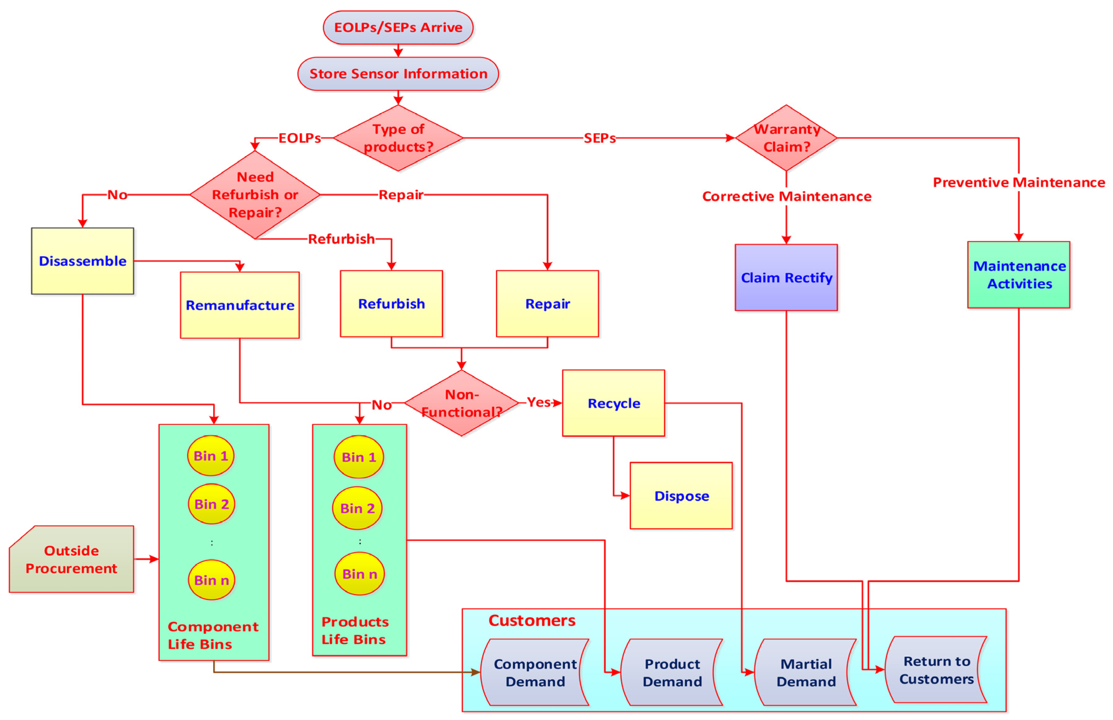
Figure 2.
Scheme for preventative maintenance (PM) policies for remanufactured Products.
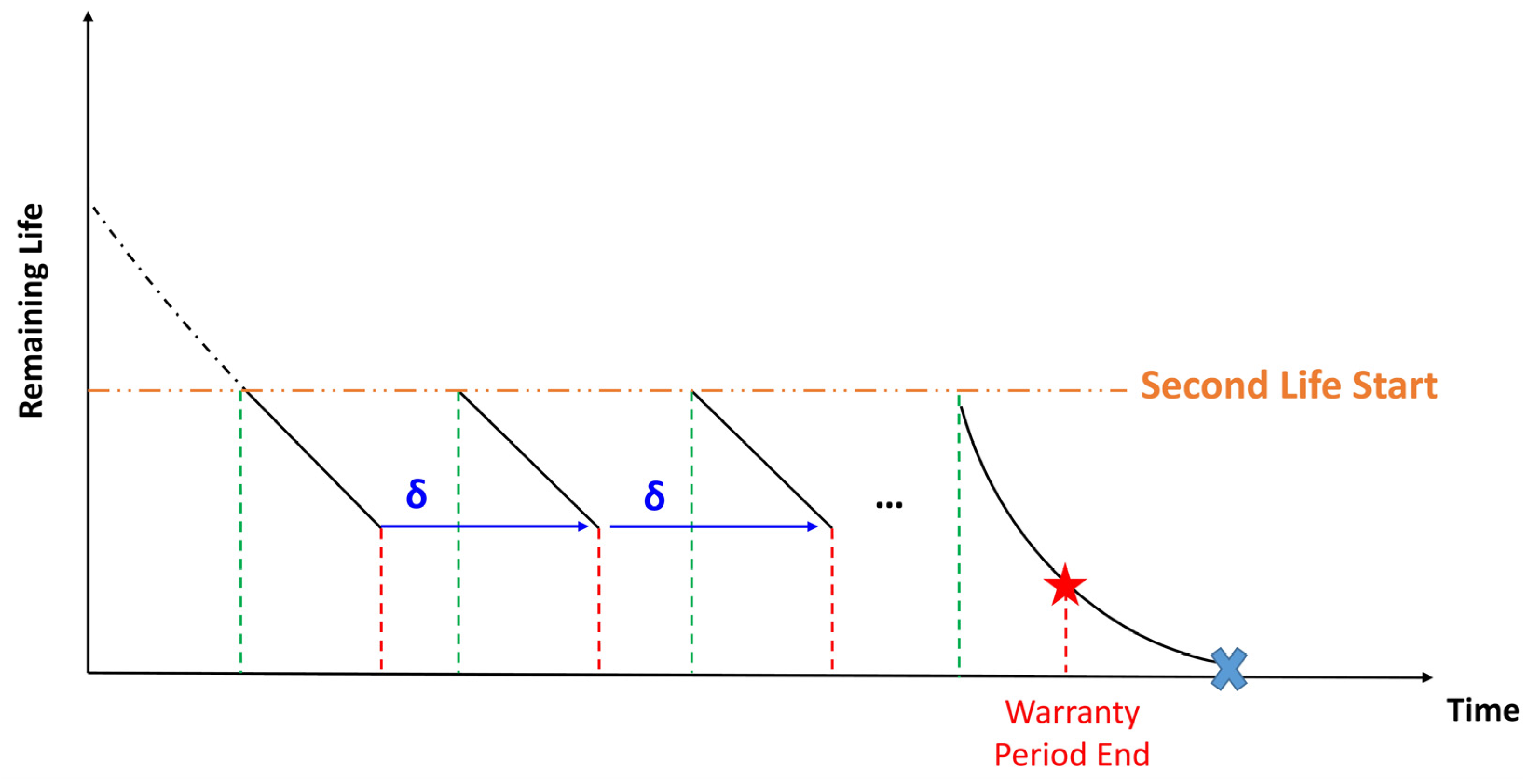
Figure 3.
One-dimensional renewing warranty policy.

Table 1.
Air conditioner (AC) Components and precedence relationship.
| Component Name | Station | Code | Preceding Component |
|---|---|---|---|
| Evaporator | 1 | A | ----- |
| Control box | 2 | B | ----- |
| Blower | 3 | C | A, B |
| Air guide | 3 | D | A, B, C |
| Motor | 4 | E | A, B, C, D |
| Condenser | 5 | F | ----- |
| Fan | 5 | G | F |
| Protector | 6 | H | ----- |
| Compressor | 6 | I | H |
Table 2.
Parameters used in the ARTO system.
| Parameters | Unit | Value | Parameters | Unit | Value |
|---|---|---|---|---|---|
| Backorder cost rate | % | 40 | Price for 3 Years Air Guide | $ | 15 |
| Holding cost rate | $/hour | 10 | Price for 3 Years Motor | $ | 60 |
| Remanufacturing cost | $ | 1.5 | Price for 3 Years Condenser | $ | 25 |
| Disassembly cost per minute | $ | 1 | Price for 3 Years Fan | $ | 20 |
| Price for 1 Year Evaporator | $ | 10 | Price for 3 Years Protector | $ | 20 |
| Price for 1 Year Control Box | $ | 20 | Price for 3 Years Compressor | $ | 65 |
| Price for 1 Year Blower | $ | 5 | Weight for Evaporator | lbs. | 8 |
| Price for 1 Year Air Guide | $ | 5 | Weight for Control Box | lbs. | 4 |
| Price for 1 Year Motor | $ | 45 | Weight for Blower | lbs. | 2 |
| Price for 1 Year Condenser | $ | 15 | Weight for Air Guide | lbs. | 2 |
| Price for 1 Year Fan | $ | 15 | Weight for Motor | lbs. | 6 |
| Price for 1 Year Protector | $ | 15 | Weight for Condenser | lbs. | 12 |
| Price for 1 Year Compressor | $ | 50 | Weight for Fan | lbs. | 3 |
| Price for 2 Years Evaporator | $ | 15 | Weight for Protector | lbs. | 3 |
| Price for 2 Years Control Box | $ | 30 | Weight for Compressor | lbs. | 6 |
| Price for 2 Years Blower | $ | 12 | Unit copper scrap revenue | $/lbs | 0.6 |
| Price for 2 Years Air Guide | $ | 12 | Unit Fiberglass scrap revenue | $/lbs | 0.9 |
| Price for 2 Years Motor | $ | 55 | Unit steel scrap revenue | $/lbs | 0.2 |
| Price for 2 Years Condenser | $ | 18 | Unit disposal cost | $/lbs | 0.3 |
| Price for 2 Years Fan | $ | 18 | Unit copper scrap Cost | $/lbs | 0.3 |
| Price for 2 Years Protector | $ | 20 | Unit Fiberglass Scrap Cost | $/lbs | 0.45 |
| Price for 2 Years Compressor | $ | 60 | Unit steel scrap Cost | $/lbs | 0.1 |
| Price for 3 Years Evaporator | $ | 20 | Price of 1 Year AC | $ | 180 |
| Price for 3 Years Control Box | $ | 35 | Price of 2 Years AC | $ | 240 |
| Price for 3 Years Blower | $ | 15 | Price of 3 Years AC | $ | 275 |
| Operation costs for Evaporator | $ | 4 | Operation costs for Condenser | $ | 1.66 |
| Operation costs for Control Box | $ | 4 | Operation costs for Fan | $ | 2.34 |
| Operation costs for Blower | $ | 2.8 | Operation costs for Protector | $ | 0.6 |
| Operation costs for Air Guide | $ | 1.2 | Operation costs for Compressor | $ | 3.4 |
| Operation costs for Motor | $ | 4 | Operation costs for AC | $ | 55 |
Table 3.
Factors and factor levels used in design-of-experiments study
| No | Factor | Unit | Levels | No | Factor | Unit | Levels | ||||
|---|---|---|---|---|---|---|---|---|---|---|---|
| 1 | 2 | 3 | 1 | 2 | 3 | ||||||
| 1 | Mean arrival rate of EOL ACs | Products/hour | 10 | 20 | 30 | 28 | Mean Assembly time for station 6 | Minutes | 1 | 2 | 2 |
| 2 | Probability of Repair EOLPs | % | 5 | 10 | 15 | 29 | Mean demand rate Evaporator | Parts/hour | 10 | 15 | 20 |
| 3 | Probability of a nonfunctional control box | % | 10 | 20 | 30 | 30 | Mean demand rate for Control Box | Parts/hour | 10 | 15 | 20 |
| 4 | Probability of a nonfunctional motor | % | 10 | 20 | 30 | 31 | Mean demand rate for Blower | Parts/hour | 10 | 15 | 20 |
| 5 | Probability of a nonfunctional fan | % | 10 | 20 | 30 | 32 | Mean demand rate for Air Guide | Parts/hour | 10 | 15 | 20 |
| 6 | Probability of a nonfunctional compressor | % | 10 | 20 | 30 | 33 | Mean demand rate for Motor | Parts/hour | 10 | 15 | 20 |
| 7 | Probability of a missing control box | % | 5 | 10 | 15 | 34 | Mean demand rate for Condenser | Parts/hour | 10 | 15 | 20 |
| 8 | Probability of a missing motor | % | 5 | 10 | 15 | 35 | Mean demand rate for Fan | Parts/hour | 10 | 15 | 20 |
| 9 | Probability of a missing fan | % | 5 | 10 | 15 | 36 | Mean demand rate for Protector | Parts/hour | 10 | 15 | 20 |
| 10 | Probability of a missing compressor | % | 5 | 10 | 15 | 37 | Mean demand rate for Compressor | Parts/hour | 10 | 12 | 20 |
| 11 | Mean non-destructive disassembly time for station 1 | Minutes | 1 | 1 | 1 | 38 | Mean demand rate for 1 Year AC | Products/hour | 5 | 10 | 15 |
| 12 | Mean non-destructive disassembly time for station 2 | Minutes | 1 | 1 | 1 | 39 | Mean demand rate for 2 Years AC | Products/hour | 5 | 10 | 15 |
| 13 | Mean non-destructive disassembly time for station 3 | Minutes | 1 | 1 | 1 | 40 | Mean demand rate for 3 Years AC | Products/hour | 5 | 10 | 15 |
| 14 | Mean non-destructive disassembly time for station 4 | Minutes | 1 | 1 | 1 | 41 | Mean demand rate for Refurbished AC | Products/hour | 5 | 10 | 15 |
| 15 | Mean non-destructive disassembly time for station 5 | Minutes | 1 | 1 | 1 | 42 | Mean demand rate for Material | Products/hour | 5 | 10 | 15 |
| 16 | Mean non-destructive disassembly time for station 6 | Minutes | 1 | 2 | 2 | 43 | Percentage of Good Parts to Recycling | % | 95 | 90 | 80 |
| 17 | Mean destructive disassembly time for station 1 | Minutes | 0 | 1 | 1 | 44 | Mean Metals Separation Process | Hour | 1 | 1 | 2 |
| 18 | Mean destructive disassembly time for station 2 | Minutes | 0 | 1 | 1 | 45 | Mean Copper Recycle Process | Minutes | 1 | 1 | 2 |
| 19 | Mean destructive disassembly time for station 3 | Minutes | 0 | 1 | 1 | 46 | Mean Steel Recycle Process | Minutes | 1 | 1 | 2 |
| 20 | Mean destructive disassembly time for station 4 | Minutes | 0 | 1 | 1 | 47 | Mean Fiberglass Recycle Process | Minutes | 1 | 1 | 2 |
| 21 | Mean destructive disassembly time for station 5 | Minutes | 0 | 1 | 1 | 48 | Mean Dispose Process | Minutes | 1 | 1 | 1 |
| 22 | Mean destructive disassembly time for station 6 | Minutes | 1 | 1 | 1 | 49 | Maximum inventory level for AC | Products/hour | 10 | 15 | 20 |
| 23 | Mean Assembly time for station 1 | Minutes | 1 | 1 | 2 | 50 | Maximum inventory level for Refurbished AC | Products/hour | 10 | 15 | 20 |
| 24 | Mean Assembly time for station 2 | Minutes | 1 | 1 | 2 | 51 | Maximum inventory level for AC Component | Products/hour | 10 | 15 | 20 |
| 25 | Mean Assembly time for station 3 | Minutes | 1 | 1 | 2 | 52 | Level of Preventive Maintenance effort | ------- | 1 | 1 | 1 |
| 26 | Mean Assembly time for station 4 | Minutes | 1 | 1 | 1 | 53 | Number of Preventive Maintenance to perform | # | 2 | 3 | 4 |
| 27 | Mean Assembly time for station 5 | Minutes | 1 | 1 | 2 | 54 | Time between each Preventive Maintenance | Months | 1 | 2 | 3 |
Table 4.
Expected number of failures and cost for remanufactured ACs and components for Renewable FRW, PRW, and Combination Policies.
Table 4.
Expected number of failures and cost for remanufactured ACs and components for Renewable FRW, PRW, and Combination Policies.
| Components | W * | Renewable Free Replacement Warranty (FRW) | Renewable Pro-Rata Warranty (PRW) | Renewable Combination FRW/PRW | |||||||||||||||
|---|---|---|---|---|---|---|---|---|---|---|---|---|---|---|---|---|---|---|---|
| Expected Probability of Failures | Expected Cost | Expected Probability of Failures | Expected Cost | Expected Probability of Failures | Expected Cost | ||||||||||||||
| RL * = 1 | RL = 2 | RL = 3 | RL = 1 | RL = 2 | RL = 3 | RL = 1 | RL = 2 | RL = 3 | RL = 1 | RL = 2 | RL = 3 | RL = 1 | RL = 2 | RL = 3 | RL = 1 | RL = 2 | RL = 3 | ||
| Evaporator | 0.5 | 0.3386 | 0.0022 | 0.0005 | $2.87 | $3.29 | $2.62 | 0.6335 | 0.0041 | 0.0009 | $4.76 | $5.45 | $4.36 | 0.2690 | 0.0017 | 0.0004 | $2.28 | $2.61 | $2.08 |
| 1 | 0.0679 | 0.0088 | 0.0040 | $3.19 | $3.60 | $2.68 | 0.1270 | 0.0165 | 0.0076 | $5.29 | $5.98 | $4.44 | 0.0539 | 0.0070 | 0.0032 | $2.53 | $2.86 | $2.13 | |
| 2 | 0.1016 | 0.0196 | 0.0137 | $4.78 | $4.75 | $2.76 | 0.1901 | 0.0367 | 0.0255 | $7.93 | $7.88 | $4.58 | 0.0807 | 0.0156 | 0.0109 | $3.80 | $3.78 | $2.20 | |
| Control Box | 0.5 | 0.3345 | 0.0021 | 0.0027 | $2.82 | $3.27 | $2.62 | 0.6259 | 0.0039 | 0.0050 | $4.67 | $5.42 | $4.35 | 0.2658 | 0.0017 | 0.0021 | $2.24 | $2.60 | $2.08 |
| 1 | 0.0719 | 0.0087 | 0.0217 | $3.32 | $3.51 | $2.66 | 0.1346 | 0.0162 | 0.0406 | $5.51 | $5.82 | $4.40 | 0.0572 | 0.0069 | 0.0172 | $2.64 | $2.79 | $2.11 | |
| 2 | 0.0975 | 0.0195 | 0.0730 | $4.72 | $4.66 | $2.74 | 0.1825 | 0.0365 | 0.1366 | $7.83 | $7.73 | $4.55 | 0.0775 | 0.0155 | 0.0580 | $3.75 | $3.70 | $2.18 | |
| Blower | 0.5 | 0.3304 | 0.0020 | 0.0141 | $1.41 | $1.32 | $1.35 | 0.6183 | 0.0038 | 0.0263 | $2.34 | $2.19 | $2.23 | 0.2625 | 0.0016 | 0.0112 | $1.12 | $1.05 | $1.07 |
| 1 | 0.0638 | 0.0089 | 0.1161 | $1.86 | $2.34 | $1.37 | 0.1194 | 0.0166 | 0.2171 | $3.07 | $3.88 | $2.28 | 0.0507 | 0.0070 | 0.0922 | $1.47 | $1.86 | $1.09 | |
| 2 | 0.0935 | 0.0198 | 0.3904 | $2.56 | $2.88 | $1.43 | 0.1749 | 0.0371 | 0.7304 | $4.25 | $4.78 | $2.37 | 0.0743 | 0.0157 | 0.3102 | $2.03 | $2.29 | $1.14 | |
| Air Guide | 0.5 | 0.3304 | 0.0009 | 0.0752 | $0.77 | $0.76 | $0.65 | 0.6183 | 0.0017 | 0.1407 | $1.29 | $1.26 | $1.07 | 0.2625 | 0.0007 | 0.0598 | $0.62 | $0.60 | $0.52 |
| 1 | 0.0476 | 0.0090 | 0.6204 | $1.12 | $1.03 | $0.71 | 0.0890 | 0.0168 | 1.1608 | $1.86 | $1.71 | $1.18 | 0.0378 | 0.0072 | 0.4930 | $0.89 | $0.82 | $0.57 | |
| 2 | 0.0853 | 0.0172 | 0.2542 | $1.49 | $1.47 | $0.76 | 0.1597 | 0.0321 | 0.4756 | $2.46 | $2.45 | $1.26 | 0.0678 | 0.0136 | 0.2020 | $1.18 | $1.17 | $0.60 | |
| Motor | 0.5 | 0.3207 | 0.0021 | 0.4020 | $2.94 | $2.82 | $2.76 | 0.6000 | 0.0039 | 0.7522 | $4.88 | $4.67 | $4.57 | 0.2548 | 0.0017 | 0.3194 | $2.33 | $2.24 | $2.19 |
| 1 | 0.0695 | 0.0087 | 0.5214 | $3.23 | $3.01 | $2.80 | 0.1300 | 0.0161 | 0.9756 | $5.36 | $5.00 | $4.65 | 0.0552 | 0.0069 | 0.4143 | $2.57 | $2.39 | $2.23 | |
| 2 | 0.0979 | 0.0198 | 0.0109 | $4.54 | $3.90 | $2.83 | 0.1833 | 0.0371 | 0.0203 | $7.53 | $6.47 | $4.69 | 0.0778 | 0.0157 | 0.0086 | $3.61 | $3.10 | $2.25 | |
| Condenser | 0.5 | 0.3341 | 0.0022 | 0.4997 | $0.92 | $0.78 | $0.77 | 0.6250 | 0.0042 | 0.9350 | $1.52 | $1.30 | $1.27 | 0.2655 | 0.0018 | 0.3971 | $0.73 | $0.62 | $0.61 |
| 1 | 0.0650 | 0.0088 | 0.5258 | $1.33 | $1.12 | $0.84 | 0.1217 | 0.0164 | 0.9837 | $2.21 | $1.86 | $1.40 | 0.0517 | 0.0070 | 0.4178 | $1.06 | $0.89 | $0.67 | |
| 2 | 0.1024 | 0.0198 | 0.0580 | $1.54 | $1.29 | $0.89 | 0.1917 | 0.0370 | 0.1087 | $2.56 | $2.15 | $1.47 | 0.0814 | 0.0157 | 0.0461 | $1.23 | $1.03 | $0.70 | |
| Fan | 0.5 | 0.3422 | 0.0020 | 0.5214 | $1.76 | $1.49 | $1.43 | 0.6403 | 0.0038 | 0.9756 | $2.92 | $2.46 | $2.37 | 0.2719 | 0.0016 | 0.4143 | $1.40 | $1.18 | $1.14 |
| 1 | 0.0748 | 0.0087 | 0.1060 | $2.43 | $1.74 | $1.46 | 0.1399 | 0.0163 | 0.1983 | $4.02 | $2.88 | $2.43 | 0.0594 | 0.0069 | 0.0843 | $1.93 | $1.38 | $1.16 | |
| 2 | 0.0984 | 0.0197 | 0.3104 | $3.02 | $2.41 | $1.54 | 0.1841 | 0.0368 | 0.5808 | $5.01 | $4.01 | $2.56 | 0.0782 | 0.0156 | 0.2467 | $2.40 | $1.92 | $1.23 | |
| Protector | 0.5 | 0.3455 | 0.0022 | 0.3715 | $0.47 | $0.36 | $0.26 | 0.6464 | 0.0041 | 0.6951 | $0.77 | $0.60 | $0.43 | 0.2745 | 0.0017 | 0.2952 | $0.37 | $0.29 | $0.21 |
| 1 | 0.0638 | 0.0087 | 0.5667 | $0.72 | $0.59 | $0.31 | 0.1194 | 0.0164 | 1.0604 | $1.20 | $0.98 | $0.52 | 0.0507 | 0.0069 | 0.4504 | $0.57 | $0.47 | $0.25 | |
| 2 | 0.0971 | 0.0198 | 0.5236 | $1.26 | $0.85 | $0.33 | 0.1817 | 0.0371 | 0.9797 | $2.09 | $1.40 | $0.56 | 0.0772 | 0.0157 | 0.4160 | $1.00 | $0.68 | $0.27 | |
| Compressor | 0.5 | 0.3337 | 0.0022 | 0.0111 | $2.04 | $1.91 | $1.83 | 0.6243 | 0.0041 | 0.0207 | $3.38 | $3.17 | $3.03 | 0.2652 | 0.0017 | 0.0088 | $1.62 | $1.52 | $1.45 |
| 1 | 0.0675 | 0.0088 | 0.0580 | $2.62 | $2.47 | $1.98 | 0.1262 | 0.0164 | 0.1087 | $4.36 | $4.09 | $3.29 | 0.0536 | 0.0070 | 0.0461 | $2.08 | $1.96 | $1.57 | |
| 2 | 0.0979 | 0.0197 | 0.5258 | $3.58 | $3.23 | $2.04 | 0.1833 | 0.0369 | 0.9837 | $5.93 | $5.36 | $3.40 | 0.0778 | 0.0157 | 0.4178 | $2.84 | $2.57 | $1.62 | |
| AC | 0.5 | 0.3968 | 0.0029 | 0.0002 | $39.88 | $38.27 | $37.92 | 0.7424 | 0.0055 | 0.0005 | $58.14 | $55.27 | $70.54 | 0.1854 | 0.0012 | 0.0001 | $30.55 | $29.40 | $29.15 |
| 1 | 0.1020 | 0.0117 | 0.0018 | $41.62 | $42.08 | $39.70 | 0.1909 | 0.0219 | 0.0034 | $60.67 | $60.78 | $73.84 | 0.0375 | 0.0049 | 0.0007 | $31.77 | $32.09 | $30.40 | |
| 2 | 0.1337 | 0.0260 | 0.0059 | $48.90 | $48.18 | $41.17 | 0.2502 | 0.0488 | 0.0111 | $71.28 | $69.60 | $76.60 | 0.0544 | 0.0110 | 0.0025 | $36.90 | $36.39 | $31.44 | |
* W = Warranty Period; RL = Remaining Life at the time of sale.
Table 5.
Results of pairwise t tests for warranty models with and without preventive maintenance.
| Performance Measure | Mean Value for Warranty Model | 95% Confidence Interval | t-Value | p-Value | |
|---|---|---|---|---|---|
| Without PM (µ1) | With PM (µ2) | ||||
| Holding Cost | $131,415.23 | $102,931.82 | 19,950<µ1 − µ2<20,757 | 98.92 | 0 |
| Backorder Cost | $26,433.25 | $20,520.79 | 5512.2< µ1 − µ2<5715.1 | 108.52 | 0 |
| Disassembly Cost | $280,261.39 | $224,079.27 | 72,494< µ1 − µ2<−75,219 | 106.31 | 0 |
| Disposal Cost | $53,066.80 | $37,813.74 | 10,988< µ1 − µ2 <11,410 | 104.04 | 0 |
| Remanufacturing Cost | $783,542.53 | $622,387.92 | 225,960< µ1 − µ2<241,214 | 60.06 | 0 |
| Transportation Cost | $27,548.28 | $21,852.85 | 5105.9< µ1 − µ2<5294.6 | 108.08 | 0 |
| Warranty Cost | $14,679.47 | $10,323.43 | 6488.0<µ1 − µ2<6631.3 | 179.57 | 0 |
| Number of Claims | 13,195 | 9667 | 4088.4<µ1 − µ2<4142.1 | 300.5 | 0 |
| PM Cost | N/A | $2383.15 | −2997.26<µ1 − µ2<−2966.92 | −385.52 | 0 |
| Total Cost | $1,316,946.95 | $1,039,909.82 | 418,092< µ1 − µ2<439,853 | 77.32 | 0 |
| Total Revenue | $2,931,949.43 | $3,093,918.49 | −353,749< µ1 − µ2<−332,031 | −61.93 | 0 |
| Profit | $1,615,002.48 | $2,054,008.67 | −767,877< µ1 − µ2<−756,496 | −262.69 | 0 |
Table 6.
Results of performance measures for different models with warranty and PM.
| Performance Measure | Mean Value with Warranty and PM Offered | |||
|---|---|---|---|---|
| Conventional Model | Sensor Embedded Model with FRW | Sensor Embedded Model with PRW | Sensor Embedded Model FRW/PRW | |
| Holding Cost | $165,476.08 | $106,754.58 | $106,754.58 | $106,754.58 |
| Backorder Cost | $30,695.56 | $21,472.93 | $21,472.93 | $21,472.93 |
| Disassembly Cost | $357,312.51 | $227,669.11 | $227,669.11 | $227,669.11 |
| Disposal Cost | $57,882.72 | $43,108.58 | $43,108.58 | $43,108.58 |
| Testing Cost | $106,572.85 | N/A | N/A | N/A |
| Remanufacturing Cost | $1,228,442.21 | $636,507.33 | $636,507.33 | $636,507.33 |
| Transportation Cost | $30,996.85 | $22,378.72 | $22,378.72 | $22,378.72 |
| Warranty Cost | $77,829.20 | $6390.68 | $14,640.00 | $10,652.80 |
| Number of Claims | 36,845 | 8483 | 10,427 | 9920 |
| Preventive Maintenance Cost | $6008.71 | $1225.79 | $2142.41 | $1858.68 |
| Total Cost | $2,101,647.53 | $1,076,048.87 | $1,088,666.42 | $1,078,036.01 |
| Total Revenue | $3,323,243.94 | $4,266,324.93 | $3,262,223.40 | $4,415,572.23 |
| Profit | $1,221,596.41 | $3,190,276.06 | $2,173,556.98 | $3,337,536.22 |
Table 7.
Results of performance measures for different models with warranty without PM.
| Performance Measure | Mean Value with Warranty (No PM Offered) | |||
|---|---|---|---|---|
| Conventional Model | Sensor Embedded Model with FRW | Sensor Embedded Model with PRW | Sensor Embedded Model FRW/PRW | |
| Holding Cost | $172,149.53 | $131,415.23 | $131,415.23 | $131,415.23 |
| Backorder Cost | $31,933.47 | $26,433.25 | $26,433.25 | $26,433.25 |
| Disassembly Cost | $371,722.48 | $280,261.39 | $280,261.39 | $280,261.39 |
| Disposal Cost | $60,217.06 | $53,066.80 | $53,066.80 | $53,066.80 |
| Testing Cost | $110,870.80 | N/A | N/A | N/A |
| Remanufacturing Cost | $1,277,983.78 | $783,542.53 | $783,542.53 | $783,542.53 |
| Transportation Cost | $32,246.92 | $27,548.28 | $27,548.28 | $27,548.28 |
| Warranty Cost | $83,298.00 | $15,104.20 | $20,201.10 | $8733.10 |
| Number of Claims | 39,380 | 12,939 | 15,150.39 | 11,497 |
| Total Cost | $2,140,422.04 | $1,317,371.68 | $1,322,468.58 | $1,311,000.58 |
| Total Revenue | $3,289,645.29 | $4,213,363.50 | $3,221,726.71 | $4,360,758.07 |
| Profit | $1,149,223.25 | $2,895,991.82 | $1,899,258.13 | $3,049,757.49 |
Table 8.
ANOVA Table and Tukey Pairwise Comparisons for Warranty Cost.
| ANOVA: Warranty Cost | |||||
| Null hypothesis | All means are equal | ||||
| Alternative hypothesis | At least one mean is different | ||||
| Significance level | α = 0.05 | ||||
| SUMMARY | |||||
| Models | Count | Sum | Average | StDev | 95% CI |
| Conventional Model | 2000 | 155,658,400 | 77,829.2 | 1264.1 | (77,786.9, 77,871.5) |
| SEP Model FRW | 2000 | 12,781,365 | 6390.68 | 412.52 | (6348.41, 6432.95) |
| SEP Model PRW | 2000 | 29,280,071 | 14,640.0 | 1026.8 | (14,597.8, 14,682.3) |
| SEP Model FRW/PRW | 2000 | 21,305,697 | 10,652.8 | 947.4 | (10,610.6, 10,695.1) |
| ANOVA | |||||
| Source of Variation | SS | df | MS | F-Value | p-Value |
| Model | 6.85556 × 10¹² | 3 | 2.28519 × 10¹² | 2,457,239.94 | 0.000 |
| Error | 7,436,123,351 | 7996 | 929,980 | ||
| Total | 6.86299 × 10¹² | 7999 | |||
| Tukey Pairwise Comparisons | |||||
| Grouping Information Using the Tukey Method and 95% Confidence | |||||
| Model | N | Mean | Grouping | ||
| Conventional Model | 2000 | 77,829.2 | A | ||
| SEP Model FRW | 2000 | 6390.68 | B | ||
| SEP Model PRW | 2000 | 14,640.0 | C | ||
| SEP Model FRW/PRW | 2000 | 10,652.8 | D | ||
Means that do not share a letter are significantly different.
Table 9.
ANOVA Table and Tukey Pairwise Comparisons for number of claims.
| ANOVA: Warranty Claims | |||||
| Null hypothesis | All means are equal | ||||
| Alternative hypothesis | At least one mean is different | ||||
| Significance level | α = 0.05 | ||||
| SUMMARY | |||||
| Models | Count | Sum | Average | StDev | 95% CI |
| Conventional Model | 2000 | 73,690,614 | 36,845.3 | 568.0 | (36,822.6, 36,868.0) |
| SEP Model FRW | 2000 | 16,967,427 | 8483.7 | 497.5 | (8461.0, 8506.5) |
| SEP Model PRW | 2000 | 20,854,626 | 10,427.3 | 505.5 | (10,404.6, 10,450.1) |
| SEP Model FRW/PRW | 2000 | 19,240,684 | 9620.3 | 500.8 | (9597.6, 9643.1) |
| ANOVA | |||||
| Source of Variation | SS | df | MS | F-Value | p-Value |
| Model | 1.10244 × 10¹² | 3 | 3.67479 × 10¹¹ | 1,365,705.09 | 0.000 |
| Error | 2,151,535,794 | 7996 | 269,077 | ||
| Total | 1.10459 × 10¹² | 7999 | |||
| Tukey Pairwise Comparisons | |||||
| Grouping Information Using the Tukey Method and 95% Confidence | |||||
| Model | N | Mean | Grouping | ||
| Conventional Model | 2000 | 36,845.3 | A | ||
| SEP Model FRW | 2000 | 8483.7 | B | ||
| SEP Model PRW | 2000 | 10,427.3 | C | ||
| SEP Model FRW/PRW | 2000 | 9620.3 | C | ||
Means that do not share a letter are significantly different.
Table 10.
ANOVA Table and Tukey Pairwise Comparisons for Preventive Maintenance
| ANOVA: Preventive Maintenance | |||||
| Null hypothesis | All means are equal | ||||
| Alternative hypothesis | At least one mean is different | ||||
| Significance level | α = 0.05 | ||||
| SUMMARY | |||||
| Models | Count | Sum | Average | StDev | 95% CI |
| Conventional Model | 2000 | 12,017,413 | 6008.71 | 193.87 | (6000.29, 6017.12) |
| SEP Model FRW | 2000 | 2,451,582 | 1225.79 | 282.39 | (1217.38, 1234.21) |
| SEP Model PRW | 2000 | 4,284,826 | 2142.41 | 129.55 | (2134.00, 2150.83) |
| SEP Model FRW/PRW | 2000 | 3,717,365 | 1858.68 | 115.26 | (1850.27, 1867.10) |
| ANOVA | |||||
| Source of Variation | SS | df | MS | F-Value | p-Value |
| Model | 28,184,227,924 | 3 | 939,4742,641 | 254,951.39 | 0.000 |
| Error | 294,645,826 | 7996 | 36,849 | ||
| Total | 28,478,873,749 | 7999 | |||
| Tukey Pairwise Comparisons | |||||
| Grouping Information Using the Tukey Method and 95% Confidence | |||||
| Model | N | Mean | Grouping | ||
| Conventional Model | 2000 | 6008.71 | A | ||
| SEP Model FRW | 2000 | 1225.79 | B | ||
| SEP Model PRW | 2000 | 2142.41 | C | ||
| SEP Model FRW/PRW | 2000 | 1858.68 | D | ||
Means that do not share a letter are significantly different.
© 2017 by the authors. Licensee MDPI, Basel, Switzerland. This article is an open access article distributed under the terms and conditions of the Creative Commons Attribution (CC BY) license (http://creativecommons.org/licenses/by/4.0/).
Share and Cite
MDPI and ACS Style
Alqahtani, A.Y.; Gupta, S.M. One-Dimensional Renewable Warranty Management within Sustainable Supply Chain. Resources 2017, 6, 16. https://doi.org/10.3390/resources6020016
AMA Style
Alqahtani AY, Gupta SM. One-Dimensional Renewable Warranty Management within Sustainable Supply Chain. Resources. 2017; 6(2):16. https://doi.org/10.3390/resources6020016
Chicago/Turabian StyleAlqahtani, Ammar Y., and Surendra M. Gupta. 2017. "One-Dimensional Renewable Warranty Management within Sustainable Supply Chain" Resources 6, no. 2: 16. https://doi.org/10.3390/resources6020016
Note that from the first issue of 2016, this journal uses article numbers instead of page numbers. See further details here.