Article

The Global Societal Steel Scrap Reserves and Amounts of Losses

Materials Science and Engineering, Applied Process Metallurgy, Royal Institute of Technology (KTH), Brinellvägen 23, Stockholm 100 44, Sweden
*
Author to whom correspondence should be addressed.
Resources 2016, 5(3), 27; https://doi.org/10.3390/resources5030027
Submission received: 30 August 2016 / Revised: 30 August 2016 / Accepted: 5 September 2016 / Published: 13 September 2016

Abstract

:
In this study a newly developed method called the Progressing and Backcasting models were used to evaluate the annual resource utilizations of steel scrap in Sweden and globally. The model results show that it is possible to assess the amounts of steel scrap available for steelmaking at a given point in time, based on statistical dynamic material flow models. By a better mapping of the available amounts of steel scrap reserves on a country basis, it is possible to ease the trade of scrap across country boarders. This in turn can optimize the supply of recyclable metals as a raw material used in the industry. The results for Swedish steel consumption show that export bans used to secure the domestic market of steel scrap do damage the internal market due to increased amounts of losses. This suggests that export bans should be lifted to optimize recycling in countries. The model results also show that the global losses of steel are higher than for an industrialized country such as Sweden. Furthermore, the results show that the Backcasting and Progressing models can be used to calculate robust forecasts on the long term availability of steel scrap assets. This information could be used for future structural plans of scrap consuming steelmaking mills and waste management facilities. Hence, it is possible to contribute to a sustainable industrial development and a circular economy.

Graphical Abstract

1. Introduction

For hundreds of centuries and still today, mineral commodities are the main raw materials used to produce metals. Over the last few decades, increased awareness of global warming and environmental degradation have created incentives to substitute natural resources with recycled scrap. However, this transition from using mineral commodities to scrap has not occurred successfully for the steel industry. From a sustainability point of view, the share of the global production of the secondary steelmaking route has instead decreased from 34% to 26% between 2000 and 2014 [1,2].
Steel is either produced by the integrated steelmaking route by using mainly natural resources of iron ore, or by using the secondary steelmaking route using recycled steel scrap. To support sustainable growth of installed capacities, information on the available amounts of reserves and resources of the raw materials used to produce metals are of importance. Specifically, this information can be used to aid the planning of investments in urban and rural mining and to obtain a stable and continuous supply of commodities used in the industry.
While information on reserves and resources of iron ore in the lithosphere are commonly available [3,4,5,6], data on the available amounts of steel scrap assets in society are not readily available information. This is due to the fact that steel scrap is generated in a wide range of different products and applications, and that there are many scrap dealers and there exists a black market of buying and selling steel scrap [7]. In addition, no statistical data on the steel scrap reserves are publicly available information at the World Steel Association and Bureau of International Recycling [8,9].
The societal steel scrap reserves are available in limited amounts dependent on the magnitude of the losses and the steel consumption in countries. Hence, the recycling rate of metals can be used to evaluate the magnitude of exchanging natural resources with recycled scrap. However, to assess the amounts of losses in society has proven to be rather difficult. Aside from the impossible task of quantifying and measuring a dissipated amount of metals, the recycling rate has been difficult to calculate due to the time aspect of the rate. To properly compare the amount of recycled scrap to its consumption stage, when the metal was consumed, requires knowledge on the wide scattering of the lifetimes of products and applications in society over time. In addition, steel has been consumed in different products and applications over the years with different alloy contents, where the lifetimes of steel have not been product specific. Thereby, it has been difficult to obtain the lifetime of steel data on an annual basis [10,11,12,13,14,15,16,17,18,19,20,21,22,23,24,25,26,27].
To secure the raw material assets of recyclable metals as a sustainable resource for the industry, long-term robust analysis is needed on the available amounts of metal scrap dependent on how assessable they are at different times. Furthermore, by better mapping of the steel scrap reserves it is possible to ease future structural plans of scrap-based steelmaking mills and waste management facilities and help keep the collection rate of steel scrap at a continuously high level. Furthermore, by utilizing steel scrap, it is possible to reduce the energy usage and CO2 emissions associated with steelmaking, preserve natural resources, and decrease the degradation of landscapes. Also, the future global reduction of greenhouse gas emissions is dependent on the act of exchanging natural resources with recyclable materials. To aid this transition, robust methods to assess the steel scrap assets in society are needed.
In a previous study, a newly developed statistical method for the annual evaluation of recycling rates in material flows called the Progressing and Backcasting models was established to enable a consistent analysis of resource utilizations [28,29]. The newly developed Dynamic Material Flow Models (DMFM) are solely based on input data on the material consumption and material collection. Furthermore, the newly developed method eliminates the need of using adjustable parameters. In this study, all input data used in DMFMs other than the material consumption and material collection are called adjustable parameters. The models are based on a study called the volume correlation model, which can be used to calculate system specific lifetimes of steel values [30]. Moreover, the model can be used to calculate the service lifetime and the time period the steel is redundant on an annual basis. In the current study, the parameters of the lifetime of steel, recycling rate, and in-use steel stock are output data [28,29]. In previous studies, these parameters are input data for the models [10,11,12,13,14,15,16,17,18,19,20,21,22,23,24,25,26,27]. The newly developed method can only be applied on consistent data series of the material consumption and material collection. The model description, methodology, and the input data used in the models were presented in previous studies [28,29,30,31].
The Progressing and Backcasting models differ from previous DMFMs with respect to three significant aspects; (i) the models are only based on input data on the material consumption and material collection; (ii) the lifetime data represents internal time-varying parameters; and (iii) the societal steel scrap reserve is segregated from the amounts of losses based on two different values on the lifetimes of steel data being used. In previous DMFMs, the input data are projected over the years based on discrete models [10,11,12,13,14,15,16,17,18,19,20,21,22,23,24,25,26]. In this study, the dynamic behavior between the parameters of the lifetimes of steel, recycling rate, and in-use steel stock per capita enables the possibility to distinguish the range of the variance of the model results on the steel scrap generation. This is due to an increased scrap collection, which over the years has lead to a decreased value of the lifetime of steel data as well as an increased recycling rate. This further contributes to a robustness of the model calculations on the steel scrap generation based on the input data of the steel consumption and scrap collection being used. These DMFMs are called statistical models since they use no additional adjustable parameters.
The focus of the present study was to investigate if the Backcasting and Progressing models can be used to (1) model how much scrap there is available for steelmaking at a given point in time? In addition, (2) make robust forecasts on the long-term availability of steel scrap assets?
The societal steel scrap reserves and amounts of losses were calculated for the Swedish steel consumption and the global steel consumption between 1900 and 2012. Thereafter, the results using the Backcasting and Progressing models were compared. This was done to evaluate if the models are complementary by calculating the upper and lower limits of the societal steel scrap reserves and amounts of losses. This represents a sensitivity analysis of the model results on the steel scrap generations based on the lifetime of steel data and the distribution functions being used. Furthermore, the models were also used to forecast the potential scrap generation and amounts of losses between 2013 and 2060. The steel scrap generations were calculated for two scenarios, namely for the same scrap collection rate as in 2012 and for a target value of the scrap collection rate. The model calculations on the forecasted input data were performed to investigate if the models can be used to calculate sustainable outlooks on the available amounts of steel scrap. Sustainable outlook refers to optimizing the recycling rate without decreasing the lifetime data of steel. This indicates that the steel scrap collection cannot be at any target level without reducing the lifetime performance of steel in society. The input data used in the models are described in a previous study [29].

2. System Boundary and Definitions

The material flow of steel and the system boundary in this study is illustrated in Figure 1. The steel is produced at steel mills and foundries by using virgin ore or recycled steel scrap as the main raw materials. The production process using iron ore is mainly represented by the blast furnace (BF) process, which uses purchased steel scrap as a cooling agent in the converters. The production processes using scrap as the main raw materials, represents the foundries as well as the electric arc furnace (EAF) process. These production processes can use up to 100% of steel scrap as raw materials. The raw materials produced from virgin ore are iron ore, sponge iron, and alloy additions. These are shown in italics in the right bottom corner of the chart shown in Figure 1.
The steel scrap is generated at different stages in society and can be divided into the following category groups of (i) home scrap; (ii) prompt scrap; and (iii) old scrap, shown in underlined italics in Figure 1. The home scrap is generated at the steel mills and foundries and is assumed to be fully recovered and consumed internally within some months. The finished steel products represent the steel product deliveries from the steel mills and foundries, which consists of casts, strips, plates, bars, pipes, tubes, and other products. The finished steel products can be directly consumed in society for different applications, mostly in the construction sector. The finished steel products can also be further manufactured and merged at external workshops into products consisting of different materials and narrow components, such as vehicles, appliances, and electronic goods. At the external workshops, prompt scrap is generated. The prompt scrap contains low contents of impurity elements and it is most often recycled within a year.
The net exports of steel containing products are illustrated in bold with double arrows pointing in opposite directions, see Figure 1. The net exports of manufactured goods (e.g., vehicles, appliances, electronic goods) are called an indirect trade, since the amount of steel is not registered as finished steel products but as product complexities. This trade is not considered in the input data on the Swedish steel consumption.
The steel consumption in society is illustrated as h t in Figure 1. It represents the finished steel product deliveries from the steel mills and foundries, but it is adjusted for the export and import values of the same product groups. The steel consumption will then reach its in-use phase (θ), where the steel will obtain a service lifetime. Note that the amounts of re-used material will elongate the lifetime of steel. This time duration is considered in the model calculations based on the so called volume correlation model [30]. After its service lifetime, the steel products will become redundant and it will reach its end-of-life (EOL) phase. This steel then enters the societal steel scrap reserve (ω), which is the stock available for collection. This amount of EOL steel is no longer used for its application purpose. However, the scrap has not yet been collected for recycling purposes. In this study, the societal steel scrap reserve is segregated from the in-use of steel based on the lifetimes of steel data. Some EOL products can also be exported to third-world countries for re-use, e.g., vehicles. This indirect trade of EOL products is not considered in the input data on the Swedish steel consumption.
Dependent on the demand of steel scrap, the EOL steel containing products will be collected and further processed and upgraded into commercial scrap. This amount of steel scrap is called an “old steel scrap”. The processing and upgrading stages of scrap at the waste management companies mainly consists of shredding, mixing, and densification of the steel scrap to ease the loading and transportation of the raw material. Both the prompt scrap and old steel scrap can be processed and upgraded at the waste management companies. The collected steel scrap represents the sum of the prompt scrap and old scrap at the stage when the scrap has been purchased and is to be consumed at the steel mills and foundries as a raw material. The steel scrap collection represents the commercial scrap which has previously been domestically used for its application purpose and the amounts of prompt scrap, which is shown as f t in Figure 1.
The losses occur at every processing stage and during the in-usage of the steel containing products and applications, and are shown as L1–L6 in Figure 1. These losses represent the quantities of steel that are not economically recoverable for recycling purposes.
The input data used in the Backcasting and Progressing models represent the steel consumption h t and scrap collection f t . The calculation methods to obtain the input data are described in a previous study [29]. The models in this study assess the in-use stock of steel (θ), societal steel scrap reserve (ω), and losses (γ) representing L1–L6 shown in the material flow in Figure 1. The losses that occur during the production process of steelmaking, shown as L1 in Figure 1, are not included in the amounts of losses in society.

3. Results and Discussion

A newly developed method called the Progressing and Backcasting models was used to evaluate the annual resource utilizations of steel scrap in Sweden and globally [29]. This newly developed method eliminates the need of using adjustable parameters. The models are solely based on input data on the material consumption and material collection. The models use time-varying internal parameters on the lifetime of steel data, given historical distributions (Backcasting model) and a normal distribution function (Progressing model) to calculate the upper and lower limits of the steel scrap generations, respectively.
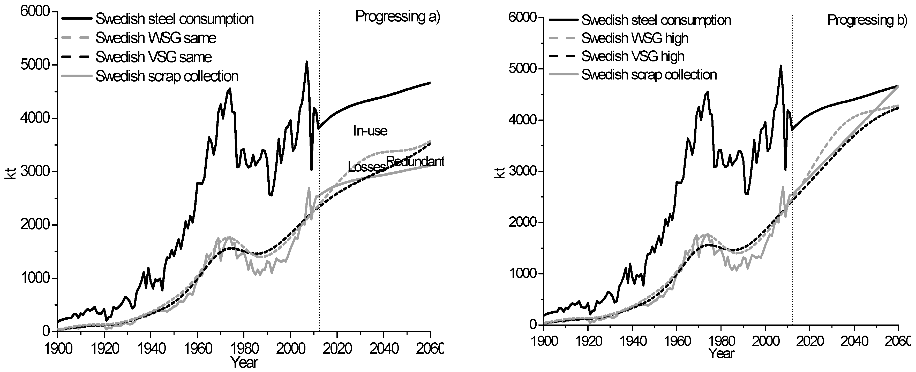
These quantities are given in the order of magnitudes and are referred to as the theoretical scrap generation (TSG), potential scrap generation (PSG), workable scrap generation (WSG), and viable scrap generation (VSG), as seen in Figure 2. The graph in 
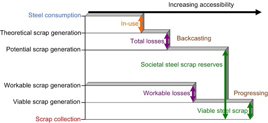
Figure 2 illustrates the relation between the model results and the different phases of steel in society. Note that the quantities and the accessibilities are in order but not scaled. The difference between the steel consumption and the TSG represents the in-use steel. The difference between the TSG and PSG values represents the amount of losses, and the difference between the PSG and the scrap collection represents the societal steel scrap reserves, as seen in Figure 2. The Progressing model calculates the lower limits on the corresponding quantities called the viable steel scrap and workable losses. The difference between the WSG and VSG values represents the workable losses and the difference between the VSG and the scrap collection represents the viable steel scrap amount. The above mentioned phases of steel are accessible in the same order, which is illustrated in the horizontal axis in Figure 2. These amounts of steel scrap assets are recoverable based on probability due to the lifetime of steel data used. This indicates that the time duration of the steel consumption in society determines when the steel will become a societal steel scrap reserve, a loss, or a collected steel scrap amount. In comparison to natural resources, these quantities are not economically feasible amounts of commodities, but statistical amounts of metal scrap assets available for collection in society. Statistical refers to the scale parameters and distribution functions used in the models. The steel scrap reserves are thereby a probabilistic amount of steel scrap available for steelmaking at a given point in time.
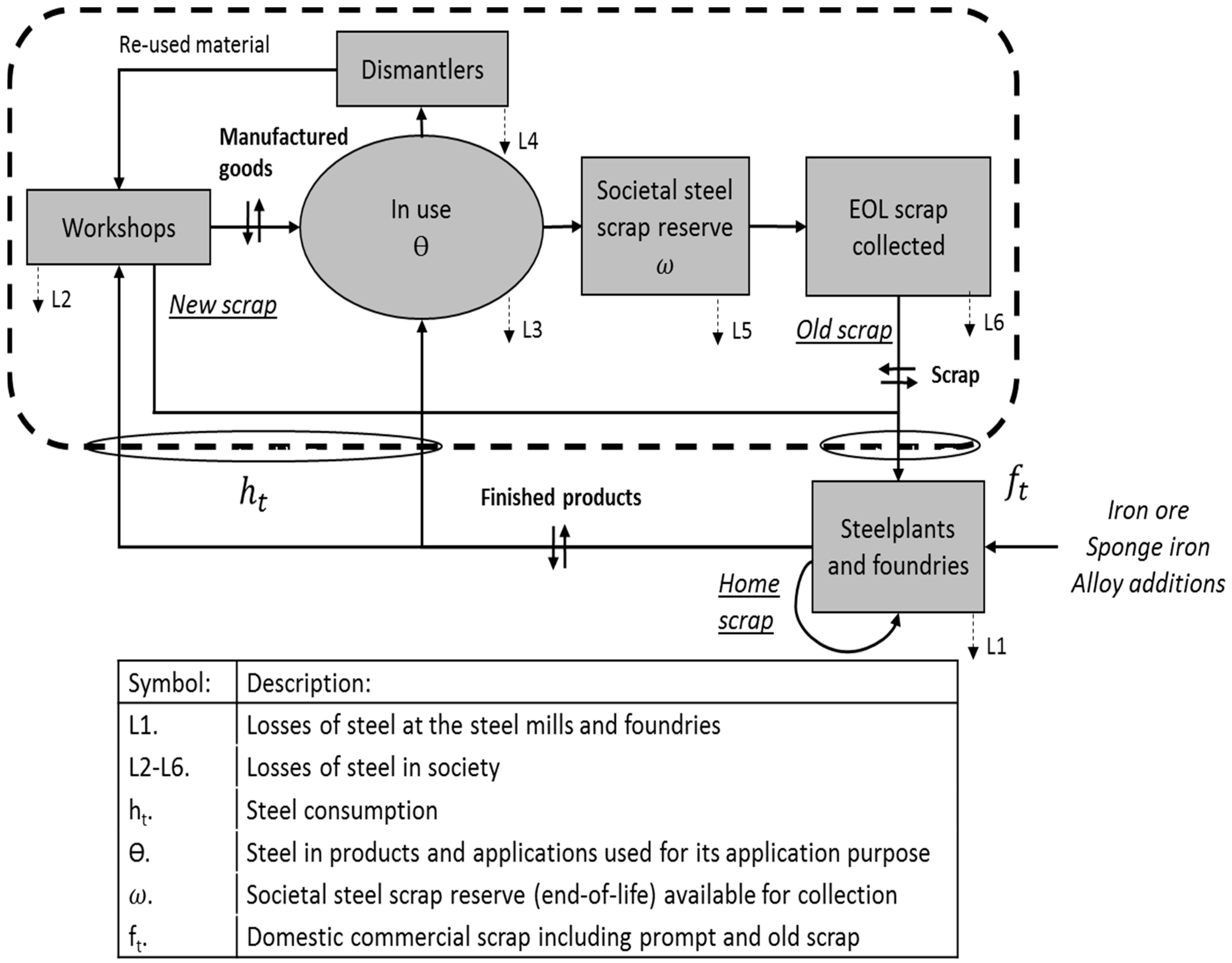
The societal steel scrap reserves represent the amount of steel that has reached an EOL stage and which therefore is available for collection. The societal steel scrap reserve is the redundant amount of steel saturated in society which is not used for its application purpose but has not yet been collected for recycling purposes. This amount of steel scrap could potentially be recovered by increased scrap prices, capacity expansions of waste management facilities, improved collection systems, etc. The lower part of the societal steel scrap reserve is called the viable steel scrap amount. The viable steel scrap can be interpreted as the economically feasible amount of steel scrap available for collection. This amount of steel scrap can be interpreted as the scrap stock available at waste management companies and collection systems in society. This amount of steel scrap is the part of the societal steel scrap reserve that is more easily accessible for recycling purposes than the redundant steel scrap in products and applications in society.
The amount of losses are the steel consumption that has been redundant for more than a period of a lifetime of steel and that are thereby not recoverable based on time. Specifically, the societal steel scrap reserves that are not recovered over a longer period of time become losses. The amount of losses can be interpreted as the non-recoverable amount of steel which is not economically feasible to collect for recycling purposes. The total losses consist of the sum of the absolute losses and the workable losses. The amount of absolute losses will not be available as a resource for the steel industry. The workable losses represent the reversible amounts of losses. This quantity has been registered as a loss, which could potentially be recoverable in the future based on the implementation of new technologies and increased scrap prices. For example, workable losses could be steel inside landfills, which due to increased scrap prices and more efficient technologies could be economically feasible to recycle in the future. The workable losses are included in the total amount of losses.
A summary with the input and output data for the Backcasting and Progressing models are shown in Table 1.

3.1. The Swedish Societal Steel Scrap Reserves and Amounts of Losses

The Progressing and Backcasting model results for the Swedish steel consumption with historical data between 1900 and 2012 and for an outlook between 2013 and 2060 for a target value on the scrap collection rate and the same scrap collection rate as in 2012 are shown in Figure 3 and Figure 4. The outlook on the higher scrap collection rate, shown in Figure 3 and Figure 4b, are calculated as the steel scrap collection to reach the same level as the steel consumption in 2060. This outlook was used to evaluate if the Backcasting and Progressing models can be used to calculate the steel scrap generation as a function of the collection rate of steel scrap. Thereby, if the models are able to calculate robust forecasts on the available amounts of steel scrap.
The Progressing and Backcasting model results show that the adaptation of the curves between the steel scrap generations and the scrap collection data, trend-wise and area-wise, are highly dependent on the distribution function that is used. This is illustrated in Figure 3 and Figure 4. The steel scrap generations calculated with a normal distribution function follow the trend of the curve of the scrap collection, as shown in the graphs in Figure 3. This is due to the fact that for a high bias distribution function, the probability of the outcome is more intense around the mean lifetime value. Furthermore, this indicates that the lifetime of the steel data calculated based on the volume correlation model is useful in DMFMs. This is due to the fact that the steel scrap generations are well adapted to the curve of the scrap collection by using the annual values on the lifetime of steel calculated based on the volume correlation model [30]. Furthermore, the model results validate the volume correlation model as a new method for calculating the lifetime of steel on a continuous basis [30].
The calculated values on the lifetime of steel are internal time-varying parameters. Thus, the Progressing and Backcasting models represent statistical models. These statistical models further contribute to a standardized way of obtaining consistent results. It should also be noted that the volume correlation model can be applied to continuous data series of any consistent stable material flow, e.g., fluid flows, energy units, patients under medication, etc.
The forecasted results based on the Progressing model between 2013 and 2060 show that the WSG and VSG seems to no longer be as well adapted to the curve of the scrap collection for a full lifetime of steel usage from the end data, see Figure 3. This is due to the fact that the lifetime of steel usage data was put as a constant value, where no data could be calculated [29]. This effect can be overcome in the future by further forecasting the input data on the steel consumption and scrap collection.
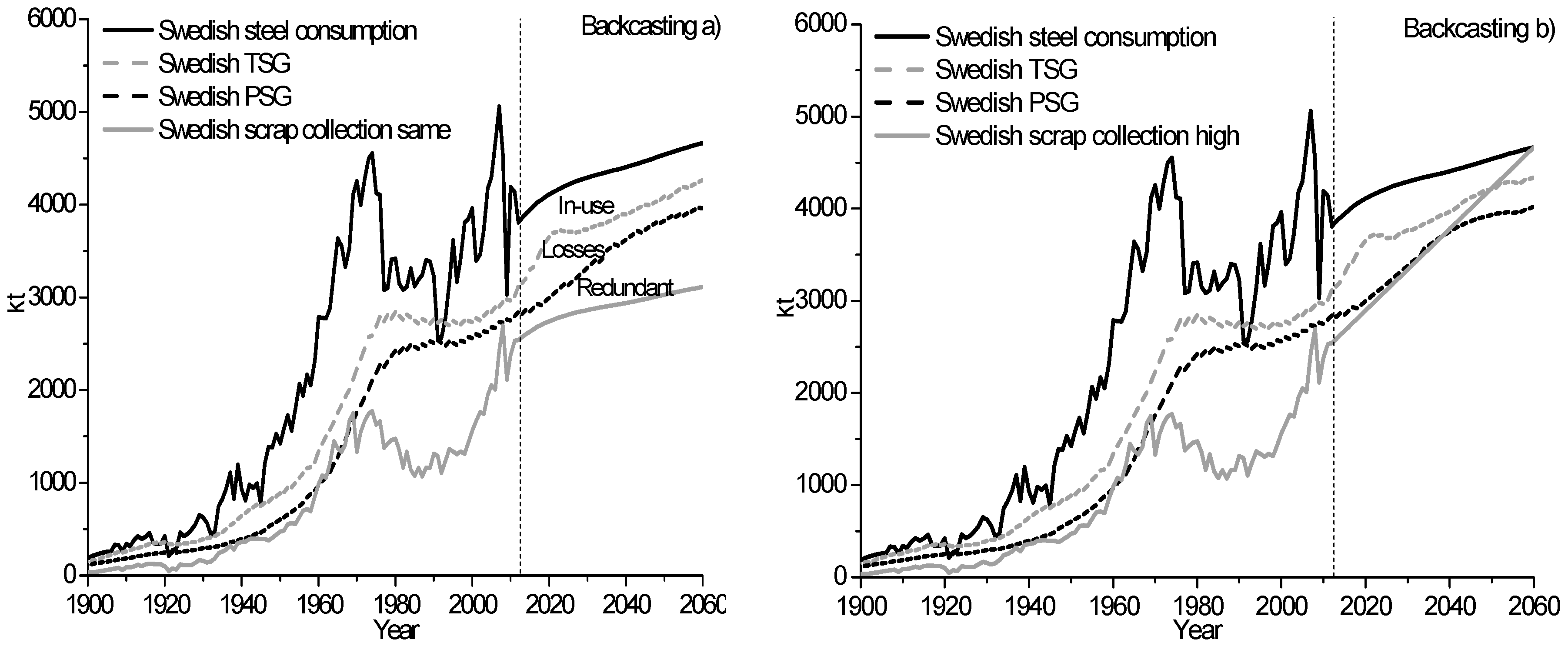
The historical results show that the societal steel scrap reserves and viable steel scrap were significantly higher between 1969 and 2010, as shown in Figure 3 and Figure 4. This can be explained by the implementation of an export ban on steel scrap between 1927 and 1993 in Sweden, which contributed to increased societal steel scrap reserves in society [32]. The model results show that the societal steel scrap reserve was higher than the demand of steel scrap to supply the Swedish steel mills for over more than four decades. During this time period the steel scrap was not utilized and instead its share was replaced by iron ore to produce steel. For the Backcasting model results shown in Figure 4, the societal steel scrap reserves are forecasted to be generated as losses around the year 2021. Specifically, about 662 kt per annum compared to 276 kt per annum in 2012. This is due to the large stock of steel scrap reserves in society. The results show that export bans to secure domestic supplies of scrap do also damage the internal market, due to increased amounts of losses. This suggests that to optimize recycling in society, export bans should be lifted.
The outlook for the Swedish steel consumption between 2013 and 2060 for two different scenarios with the same scrap collection rate as in 2012 and a higher scrap collection rate, reaching the same level as the steel consumption in 2060, is shown in Figure 4. The results show that if the demand of steel scrap is kept at the same rate as in 2012, the societal steel scrap reserves and losses will increase significantly over the upcoming years. Thus, to utilize steel scrap, the collection rate of steel scrap has to be increased to compensate for the historical large amount of societal steel scrap reserve in society. Furthermore, the outlook of the high scrap collection rate shows that the forecasted demand of steel scrap exceeds the potential scrap generation in 2039. This shows that it is not possible that the available amounts of steel scrap would reach the same level as the steel consumption in 2060 in Sweden. More specifically, the forecasted high scrap collection value exceeds the limits of what the model considers as a sustainable value. This differs from economic price-driven models that calculate unlimited amounts of metal scrap assets, just if the demand would be high enough. This is due to the fact that they are not limited in availability due to the steel consumption in society. This indicates that for evaluating the metal scarcity, economic models are not sufficient enough. The present model results show that the Backcasting model can be used to evaluate sustainable outlooks on the available amounts of steel scrap. Sustainable outlook refers to optimizing the recycling rate without decreasing the lifetime of steel in society. These robust forecasts of the steel scrap generations can be used to ease future structural plans of steelmaking. Thereby, it is possible to keep the collection rate of steel scrap at a continuous high level.
The forecasted model results show different outputs on the TSG, PSG, WSG, and VSG values, dependent on the forecasted scrap collection value that was the same or higher than the value in 2012. This shows that the Backcasting and Progressing models are able to calculate the steel scrap generations as a function of the collection rate of steel scrap. This differs from previous DMFMs that have used adjustable parameters on sector-specific single value data on the lifetime of steel as the basis for the model predictions. Thereby, the forecasted steel scrap generation has reached the same level regardless of the increase in the demand of steel scrap over the years. This is due to an increased scrap collection that has not decreased the lifetime of steel data used in the previous DMFMs. More specifically, in previous models the input data of the lifetime of steel and distribution functions have been projected over the years, while the Progressing and Backcasting models are able to distinguish the interactions between the parameters on the recycling rate, lifetime of steel, and the in-use steel stock. The results show that the new models can be used to calculate robust forecasts on the long-term availability of steel scrap. This information is of importance when planning future installations of scrap consuming steelmaking mills and waste management facilities, for evaluations of future demands of steel to industrialize countries, as well as to calculate resource limitations associated with steelmaking.
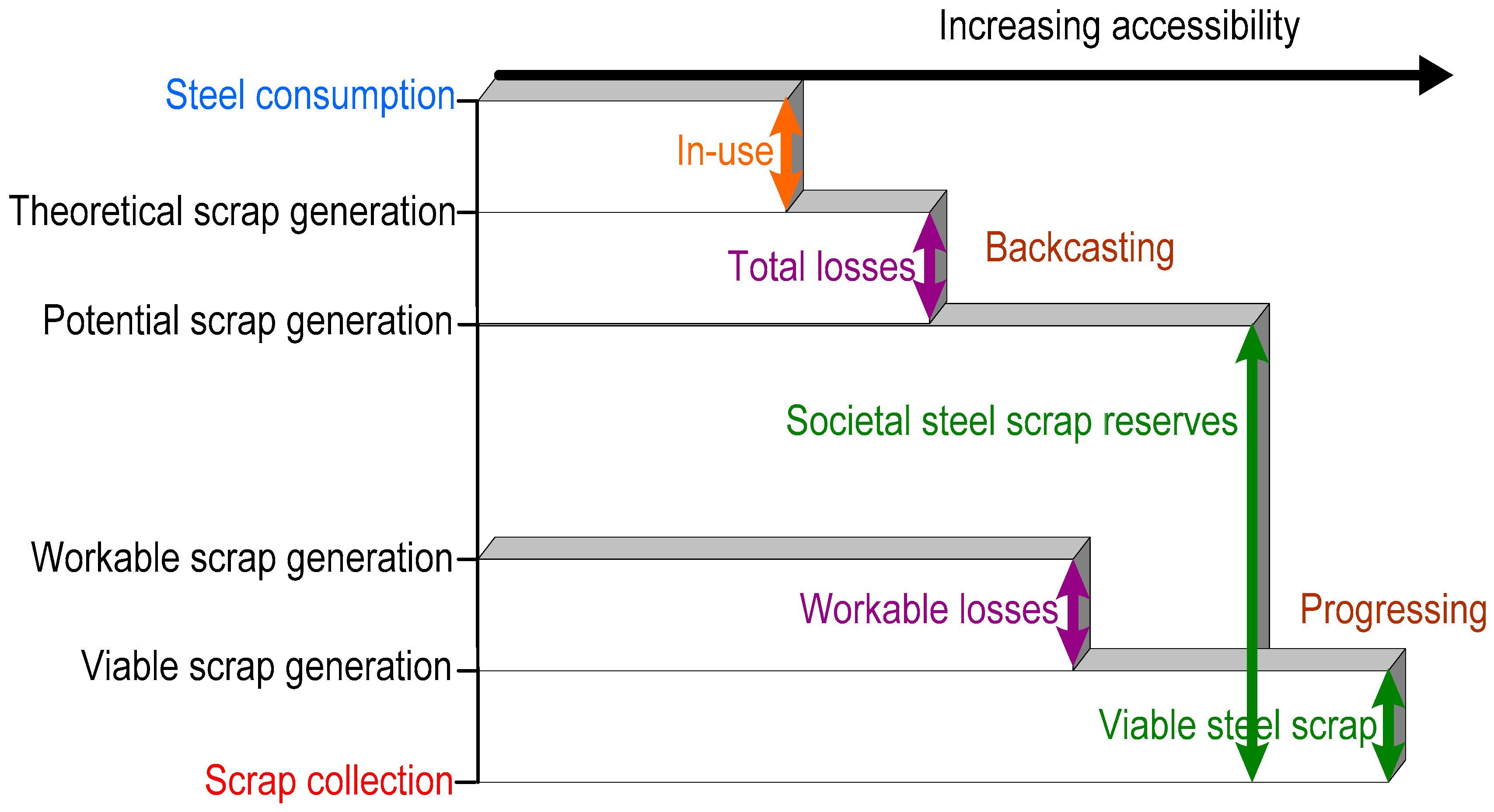
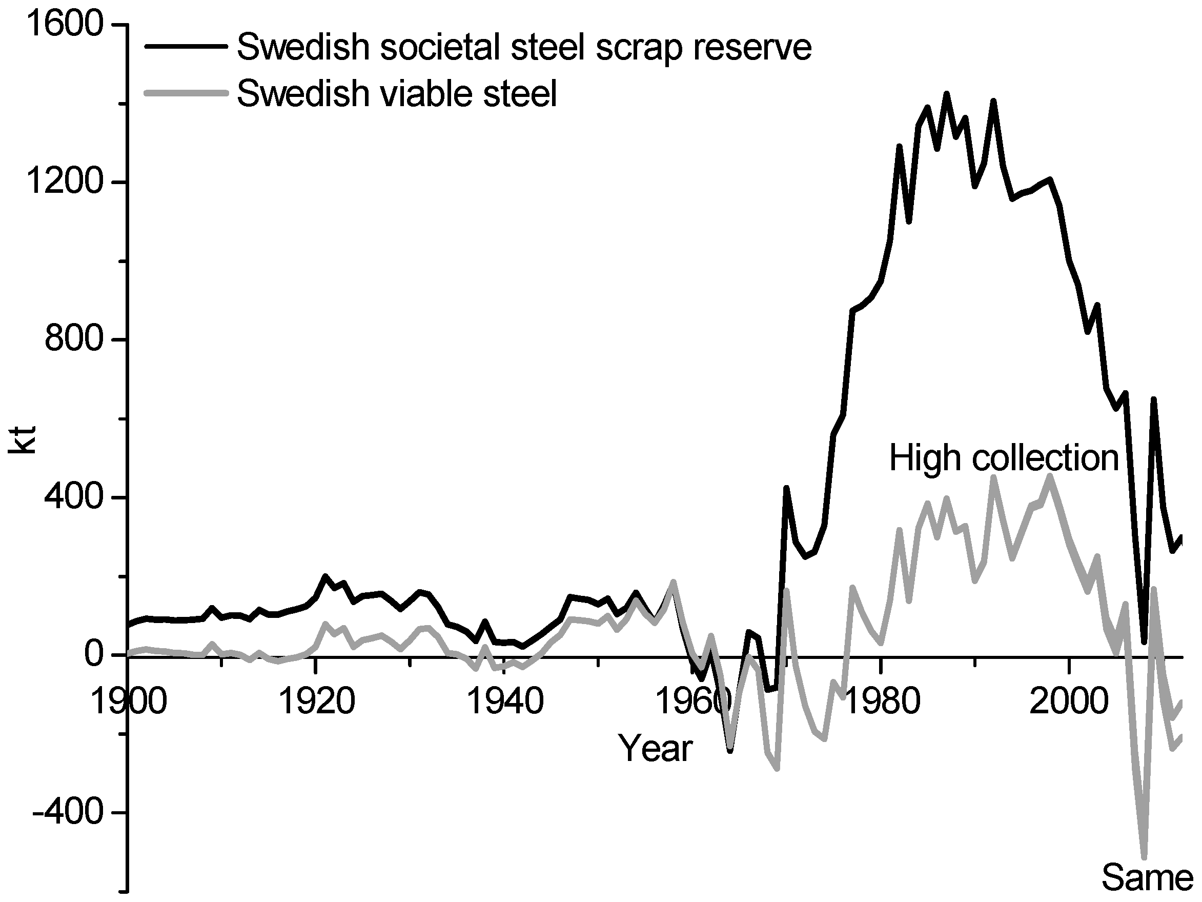
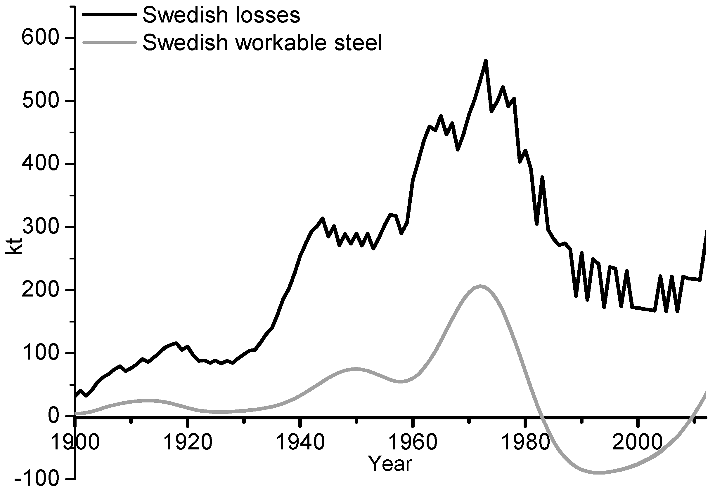
The annual quantities of the Swedish societal steel scrap reserves and amounts of losses are shown in Figure 5. These quantities are calculated based on the Backcasting model and are taken from Figure 4. The results show that the new model is able to segregate the non-recirculated amount of steel into the societal steel scrap reserves available for future collection and the amount of losses. This differs from previous material flow models that have not been able to distinguish the quantities apart based on statistics. Statistics refer to the scale parameters and distribution functions used in DMFMs. This is due to previous models that have used sector-specific single-value data on the lifetime of steel. Based on the model results, it is thereby possible to evaluate the potential of increasing the recycling of steel scrap in society. The figure shows that the most fluctuating quantity of the non-recovered amount of steel is the size of the societal steel scrap reserves. The results also show that the amount of losses are never below zero. The positive amount of losses indicates that the model follows the second law of thermodynamics. Specifically, the historical results show that the losses of steel reached the highest value of around 500 kt in 1975 and that they thereafter have decreased gradually to 277 kt in 2012. The decreased quantity of losses can be explained by increased installations of scrap consuming steelmaking facilities and the introduction of the continuous casting technique. These changes increased the demand of purchased steel scrap in the steelmaking mills. Furthermore, it can be explained by improved sorting techniques e.g., fragmentation facilities, that have increased the capacity of scrap production at the waste management companies.
The historical results also show that the societal steel scrap reserves had the highest value of around 1424 kt in 1987. Thereafter, the societal steel scrap reserves and losses have significantly decreased. This is due to the lifting of the export ban of steel scrap in 1993 in Sweden. Also, the model results show that the large amounts of societal steel scrap reserves will be generated as losses around year 2021. This is regardless if the forecasted scrap collection rate is the same or higher than it was in 2012. The model results demonstrate that the collection rate of steel scrap should be continuously high to decrease the amount of losses in society.

3.2. The Global Societal Steel Scrap Reserves and Amount of Losses

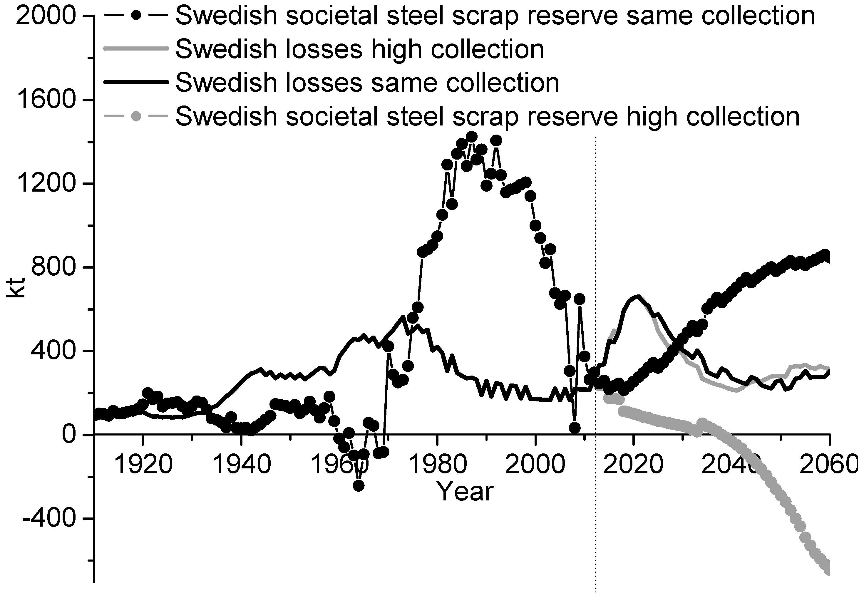
The model results on the global steel consumption for historical data between 1910 and 2012 as well as the outlook between 2013 and 2060 for both a high scrap collection rate and the same scrap collection rate as in 2012 are shown in Figure 6 and Figure 7. The Progressing model results on the upper limit of in-use steel stock, workable losses, and viable steel scrap are shown in Figure 6. The Backcasting model results on the in-use steel, societal steel scrap reserves, and amount of losses are shown in Figure 7.
The results show that for a whole century between 1910 and 2012, the TSG and PSG values have been higher than the scrap collection values, as is shown in Figure 7. Between 1910 and 1987 the amount of losses has also been higher than the collected amount of steel scrap. In addition, the societal steel scrap reserves have increased during the last four decades. Overall, the model results show that the societal steel scrap reserves and amount of losses are high in the world. This indicates that there is a need for a drastic increase as well as a better utilization of steel scrap on a country basis. This can be achieved by increased installations of the EAF route of steelmaking, by improved collection systems, and by increased installations of waste management facilities. Thus, it is of great importance to locate the societal steel scrap reserves on a country basis.
Due to economic benefits and decreased environmental impacts for the steel producers with the implementation of and increased recycling of steel scrap, scrap collection should be relatively high in the world. Despite incentives, the model results show that a large difference still exists between the collected steel scrap and the societal steel scrap reserves which are available in society.
However, the societal steel scrap reserves are accessible to different extents and amounts, dependent on how profitable it is to recycle the steel. It is thereby of great importance to evaluate where the societal steel scrap reserves are saturated in society. This can be done by calculating the steel scrap reserves by specific industrial sectors in society.
The lower limit on the steel scrap generation calculated based on the Progressing model can be interpreted as the most commonly available steel scrap assets in society. The information on the economically feasible amounts of steel scrap available for collection can be used to optimize the recovery, without improving the existing collection system in society or by increasing the installed capacity of waste management facilities. Thereby, it is possible to avoid supply bottlenecks. This could potentially further aid to stabilize the volatility effect of the raw materials used for steelmaking. The Progressing model results shows that the viable steel scrap started to be generated in larger quantities between 1977 and 2007, as seen in Figure 6. In addition the viable steel scrap peaked in 2009 due to the economic crisis.
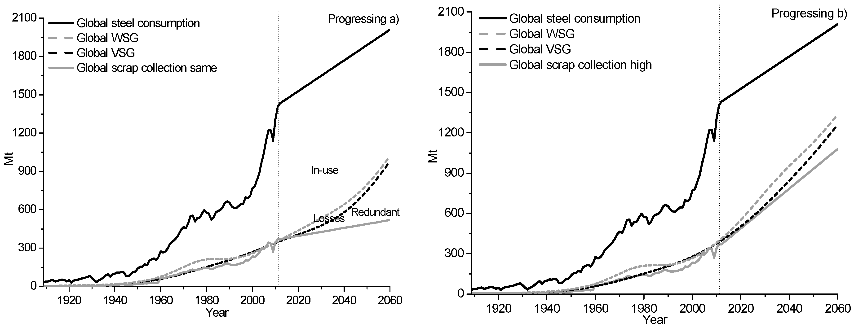
Based on the Progressing and Backcasting models, the forecasted steel demand was calculated to reach a level of 2010 Mt in 2060. This shows that the world will consume double the amount of steel up to the year 2060 compared to the total historical consumption until today. Furthermore, depending on what production process the steel will be produced by, it will have a huge impact on the environment. The recycling rate of steel is directly related to the global installed capacity of scrap consuming steelmaking mills. Considering that, the global environmental issue regarding CO2 emissions and energy usages can to a large extent be solved by an increased recycling of metal, but this requires among other actions robust models to be able to calculate the societal scrap reserves. Furthermore, by mapping the steel scrap reserves, it is possible to ease the trade of steel scrap across country borders. Hence, it is possible to optimize the global supply of steel scrap for steelmaking. This would further enable an optimized usage of recyclable metals as sustainable resources for the industry.
The forecasted steel demand can also be calculated based on mathematical functions such as the Box-Jenkins function, exponential smoothing, and regression analysis [33]. These calculations are mainly based on the data on scrap collection from the past as well as present data. Furthermore, on their historical trends, on assumptions based on experience, industrial knowledge, and financial indicators [34]. However, the projections are also time dependent, whereby the potential of increasing the recycling rate of steel also needs to be considered when evaluating the amounts of steel that will be consumed in the future. The Backcasting and Progressing models are able to distinguish the relationship between the dynamic behaviors of the lifetime of steel, recycling rate, and in-use steel stock. The use of the new models improves the forecasting of the available amounts of steel scrap as well as the demand of steel to industrialize countries.
The outlook on the global steel consumption between 2013 and 2060 for two scenarios, using the same scrap collection rate as in 2012 and a high scrap collection rate, are shown in Figure 6 and Figure 7. The results show that if the scrap collection rate is the same as in 2012, the societal steel scrap reserves will significantly increase in the upcoming years. Finally, the societal steel scrap reserves will surpass the amounts of scrap collected in the year 2048, as seen in Figure 7. The results also show that despite a higher scrap collection rate, the amount of losses will still be high in the future. This can be explained by the fact that the societal steel scrap reserves have continuously been high in the world. Also, the large amounts of losses are shown as the large difference between the TSG and PSG values in 2060, as seen in Figure 7. To maintain a global high collection rate of steel scrap, the steel scrap collection should follow the forecasted PSG value. Based on the information on the potential scrap generation, it is possible to ease future structural plans of scrap based steelmaking mills and waste management facilities. Thereby, it is possible to keep the collection rate of steel scrap at a continuously high level. This would further aid to delay as well as to minimize the usage of natural resources for steelmaking in the future.
Both the model calculations for the Swedish steel consumption and global steel consumption show that the forecasted model results are different for the TSG, PSG, WSG, and VSG, dependent on the forecasted demand of steel scrap. Thereby, the Backcasting and Progressing models are able to calculate the steel scrap generations as a function of the collection rate of steel scrap. This is based on time-varying internal parameters on the lifetime of steel data. Furthermore, the models use no additional external parameters. These statistical models enable the possibility to evaluate the relation between the recycling rates of steel against the in-use steel, the societal steel scrap reserves, and the amounts of losses over time. This is due to the fact that these quantities influence each other. Based on the information of the potential scrap generation and based on the assumption of a maximized EAF capacity, it is possible to calculate the future demand of iron ore to produce steel.
In a previous DMFM study by J. Oda et al., the old scrap consumption value was calculated to be 859 Mt and the prompt scrap consumption value was forecasted to be 209 Mt in 2060 [26]. This is a total value of 1068 Mt of commercial steel scrap that is forecasted to be consumed in the iron and steel mills. In this study, the scrap collection (old and prompt) was calculated to reach a target value of 1081 Mt in 2060. This value is very similar to the results found in the previous study by J. Oda et al [26]. However, the model results from this study also show that there exists an even greater potential of increasing the scrap collection to a value of 1261 Mt in 2060. This is shown as the potential scrap generation value in 2060 in Figure 7b. In another DMFM study by S. Pauliuk et al., the old and prompt scrap supply was calculated to be approximately 1470 Mt in 2060 [27]. This is higher than the results calculated based on the Backcasting model; specifically, 400 Mt higher than the potential scrap generation in 2060. The difference can be explained because the study by S. Pauliuk et al. assumed a target value of the End-of-life recycling rate to be 90% in 2050 [27]. This is 13% higher than the recycling rate calculated based on the Backcasting model and 37% higher than the EOL-RR calculated by J. Oda et al. for the same year [26,28].
The model results demonstrate that it is possible to assess the steel scrap generation in society based on the statistical DMFMs. Also, based on the newly developed Progressing and Backcasting models, it is possible to calculate robust forecasts on the long term availability of steel scrap.
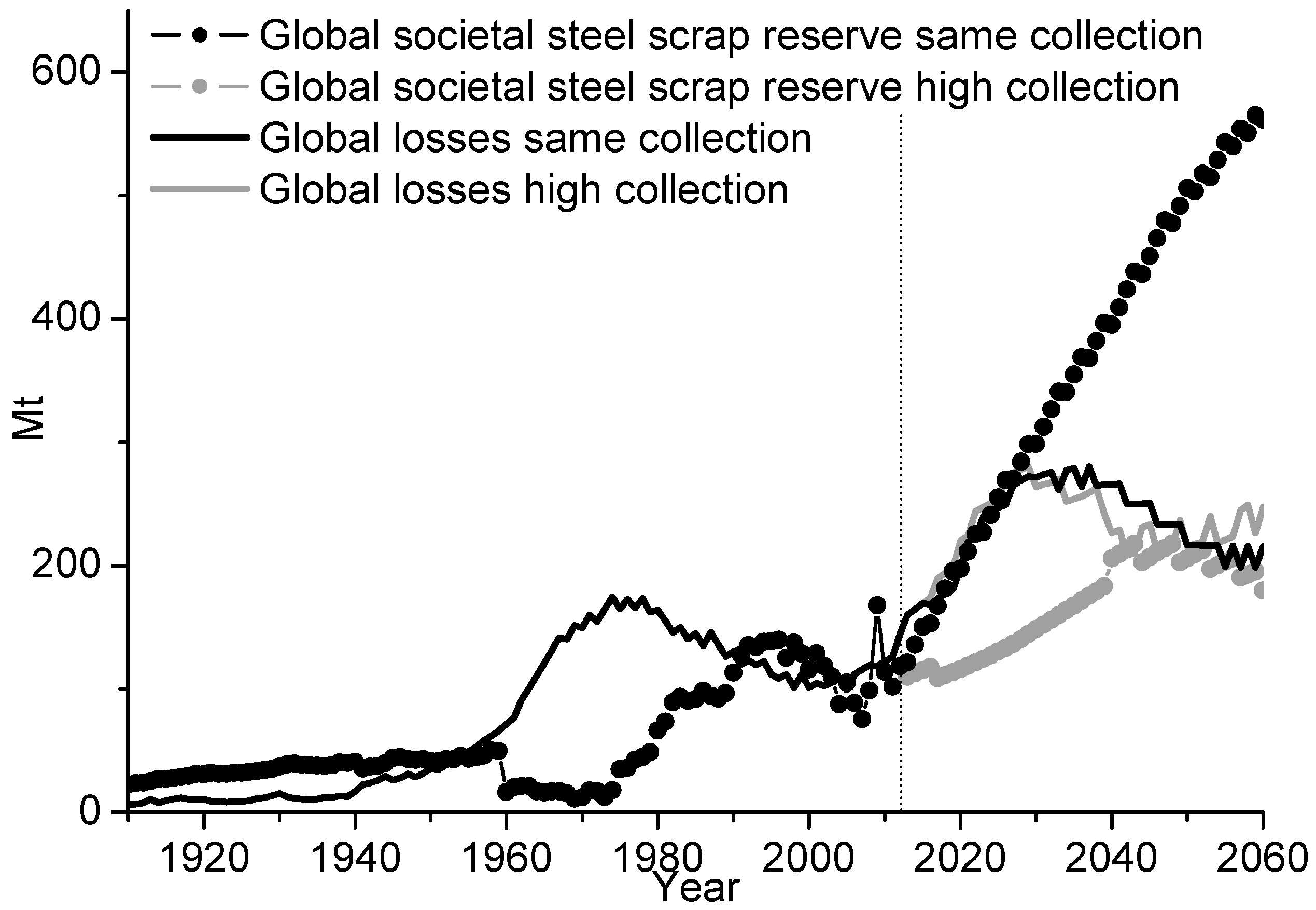
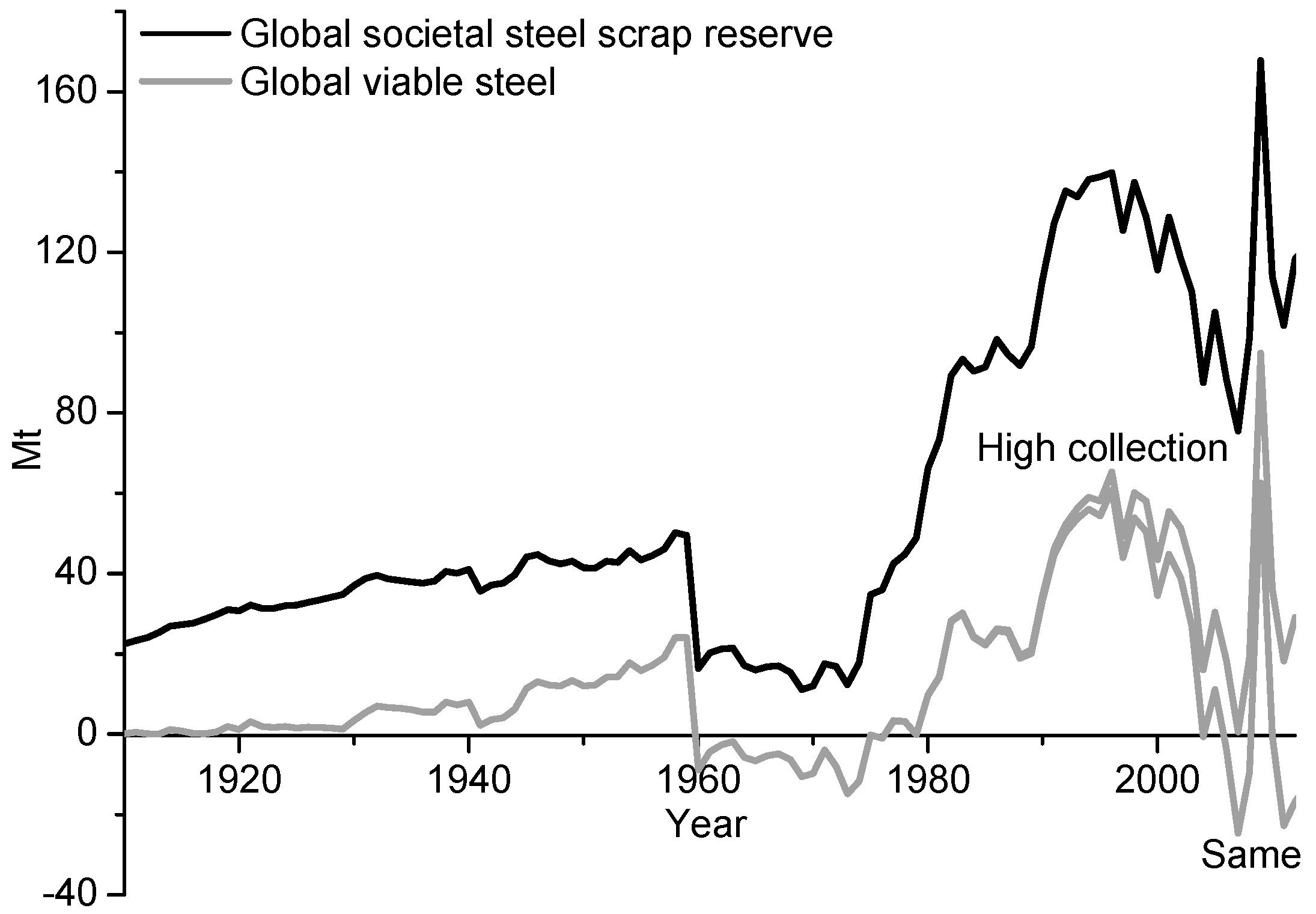
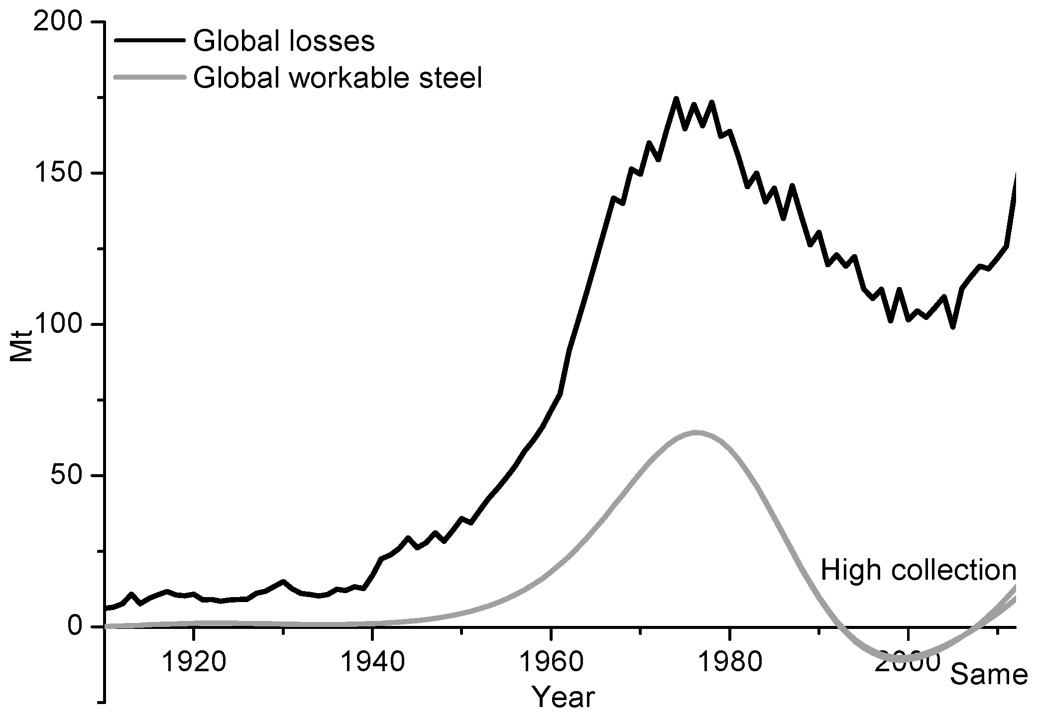
The annual quantities of the global societal steel scrap reserves and amounts of losses are shown in Figure 8. These quantities are calculated based on the Backcasting model and are taken from Figure 7. The historical data show that the cumulative amounts of the societal steel scrap reserves have been higher than the losses until 1968, after which the amounts of losses have been higher than the societal steel scrap reserves. In addition, the results also show that the amounts of losses will significantly increase in the future and that they will be around 280 Mt in 2029 and thereafter will decrease to a value between 215 and 247 Mt in 2060. This result is true regardless if a higher or the same scrap collection rate as in 2012 is assumed. However, according to the model calculations, it is necessary to keep the collection rate at a continuously high level, to reduce the amounts of losses. This can be achieved by assessing the available amounts of steel scrap in society. Furthermore, the forecast shows that there exists a great potential to decrease the amount of the societal steel scrap reserves to a level below the amounts of the losses in 2060.
The model results for the Swedish and global data between 1900 and 2012 also show that the societal steel scrap reserves and amounts of losses are counterbalancing each other, as seen in Figure 5 and Figure 8. This is because the amount of losses is a function of the societal steel scrap reserves. The losses represent the amounts of the end of life steel that have been redundant for more than a lifetime of steel and that then have become part of the losses in society. Specifically, the losses represent the quantity of steel that is statistically outside the range of being collected for recycling purposes.
Due to the fact that steel scrap is a scarce resource, supply bottlenecks can occur. This can further cause sudden changes of the prices of raw materials used for steelmaking. The collection rate of steel scrap in countries have previously not hit the ceiling of its limitation of available reserves. This excludes temporarily and local situations, when countries have implemented export bans on steel scrap to secure their domestic scrap market. With a better mapping of the steel scrap reserves, it is possible to evaluate how much steel scrap can be purchased before scrap prices would peak due to supply bottlenecks. It is thereby of great importance to assess the amounts of available steel scrap reserves in society. This in turn would help to obtain a sustainable industrial development and a circular economy.

3.3. The Lower and Upper Limit of the Societal Steel Scrap Reserves and Amounts of Losses

The societal steel scrap reserves are accessible for collection to different extents and amounts depending on how economically viable it is to recycle the steel. Therefore, it is important to quantify the lower and upper limits of the societal reserves of steel scrap and losses. The model results on the amounts of the societal steel scrap reserves, viable steel scrap, amounts of losses, and workable losses for the Swedish steel consumption and global steel consumption between 1900 and 2012 are shown in Figure 9, Figure 10, Figure 11 and Figure 12, respectively. These quantities are taken from the model results shown in Figure 3, Figure 4, Figure 6 and Figure 7.
The model results show that the societal steel scrap reserves and the viable steel scrap follow each other’s trends to a lower and upper magnitude, respectively. This is shown for both the Swedish steel consumption and the global steel consumption data. The results show that the Backcasting and Progressing models are complementary. Furthermore, the models are able to calculate the range of the statistical outcome of the available steel scrap assets in society. The combined use of the models thereby represents a sensitivity analysis on the possible outcomes of the steel scrap generations based on the lifetime of steel data and the distribution functions being used. The results show that the amounts of the societal steel scrap reserves and viable steel scrap converge and diverge over the century. However, the difference between the amounts of losses and workable losses are more continuous over time. According to the model calculations, there exists a greater potential to recover the societal steel scrap reserves and viable steel scrap assets in society compared to the amounts of losses and workable losses.
The results show that the cumulative societal steel scrap reserves are larger than the cumulative amounts of losses in Sweden in 2012, while the global cumulative losses are larger than the cumulative societal steel scrap reserves in 2012. The global results show that the cumulative losses surpassed the cumulative steel scrap reserve in 1968, as seen in Figure 11 and Figure 12. Thereafter, the global losses have been higher than the societal steel scrap reserves. Furthermore, the results show that there exists a great potential to increase the collection of the available scrap reserves in the world. An implemented scrap utilization would decrease the energy usage as well as the CO2 emissions associated with steelmaking.
In Figure 10 and Figure 12 it is shown that the Swedish workable losses and global workable losses have been negative between 1984 and 2008 and between 1998 and 2012, respectively. This indicates that new technologies to handle the amounts of workable losses had been introduced and installed. These new technologies could be installations of the fragmentation facilities, which have further increased the production of steel scrap. The workable losses could be e.g., steel in narrow components, which have been difficult and costly to process into scrap that can be recycled. However, due to increased scrap prices and newly developed technologies it is now economical to recover these sources for recycling purposes.

4. Conclusions

Two complementary statistical DMFMs, called the Progressing and Backcasting models, have previously been developed to enable assessments of the resource utilization of steel scrap. The focus of this study was to investigate if it was possible to use the Progressing and Backcasting model (1) to model how much scrap is available for steelmaking at a given point in time and (2) to make robust forecasts on the long term availability of steel scrap assets. From the results of this study, the following main conclusions can be made:
(1) It is possible to calculate the societal steel scrap reserves and amounts of losses in countries based on the statistical DMFMs.
The results show that the Backcasting and Progressing models can be used to calculate the upper and lower limits of the societal steel scrap reserves and amounts of losses, respectively. Also, the results show that export bans used to secure domestic markets of steel scrap are harmful in that they increase the amounts of losses. To optimize recycling in countries, export bans should be lifted. The results show that the global societal steel scrap reserves and amounts of losses are relatively high compared to an industrialized country such as Sweden. This indicates that there exists a great potential to increase the recycling of steel scrap in the world.
(2) It is possible to make robust forecasts on the long-term availability of steel scrap assets based on the Progressing and Backcasting models.
For these models, the steel scrap generations were shown to be a function of the collection rate of steel scrap. This indicates that the models are able to distinguish the dynamic behavior between the parameters on the lifetime of steel, recycling rate, and in-use steel stock. Furthermore, this improves the forecasting of the availability of recyclable metals as a resource available for the steel industry. The information on the potential scrap generation can be used for future structural plans of scrap consuming steelmaking mills and waste management facilities. Hence, it is possible to contribute to a sustainable industrial development and a circular economy.

Acknowledgments

The authors would like to thank MISTRA, the foundation for strategic environmental research, for their financial support. The authors would also like to thank Jernkontoret’s environmental research program “The Steel-Eco Cycle”, for the valuable inputs and comments. The authors would also like to thank Axel Hultgren’s foundation, Vinnova Sweden’s innovation agency, the Hugo Carlssons foundation, the A H Göranssons foundation, the Olle Erikssons foundation, and the Gerhard von Hofstens foundation, for their financial support.

Author Contributions

Alicia Gauffin performed all of the literature survey and methodology, a majority of the data analysis, parts of the modeling in this study, and a major part of the writing. Nils Å. I. Andersson did some parts of the writing and major parts of the program coding. Per Storm, Anders Tilliander, and Pär G. Jönsson performed parts of the writing and analysis of the model results.

Conflicts of Interest

The authors declare no competing financial interest.

Nomenclatures

Steel consumptionFinished steel products production in society corrected for the export and import of the same product groups.
Scrap collectionPurchased old and prompt steel scrap used for steelmaking, adjusted for export and import of steel scrap. Collected amounts of domestic prompt and old steel scrap.
Steel scrap reservesThe amount of steel that has reached an EOL stage and which is available for collection. The redundant amount of steel saturated in society which is not used for its application purpose but has not yet been collected for recycling purposes.
RedundantThe stage when products and applications reach their end-of-life phase and are no longer in-use for their application purpose.
LossesThe societal steel scrap reserves that have been redundant for more than a lifetime of steel and that is not recoverable due to statistics. Specifically, the losses can be interpreted as the end-of-life steel that is not economically feasible to collect for recycling purposes.
Viable steel scrapThe statistically feasible amount of steel scrap available for collection. This amount of steel can be interpreted as the scrap stock available at the waste management companies and collection systems in society. The viable steel scrap is a part of the societal steel scrap reserves.
Workable lossesThe amount of losses that potentially could be recycled in the future based on new technology. The workable losses are the reversible amounts of losses and are included in the total amount of losses in society.
In-use steel stockThe total amount of steel consumed in countries to build up the infrastructure and the steel consumed in products and applications. The in-use steel stock is the functional amount of steel that is used for its application purpose.
Recycling rate (RR)The ratio of the scrap collection divided by the sum of the amount of losses and scrap collection (RR). 100% minus the RR value corresponds to the ratio of the losses.
Theoretical scrap generation (TSG)The sum of the societal steel scrap reserves, amount of losses, and collected scrap.
Potential scrap generation (PSG)The sum of the societal steel scrap reserves and collected scrap.
Workable scrap generation (WSG)The sum of the viable steel scrap, amount of workable losses, and collected scrap.
Viable scrap generation (VSG)The sum of the viable steel scrap and collected scrap.
Mineral ReserveOre reserves that are legally, economically, and technically feasible to extract.
Mineral ResourcePotentially valuable amounts of resources that could be available in the future for economic extraction.
BackcastingTo apply the lifetime of End of life steel data on the scrap collection and evaluate the magnitude of the scrap collection to the steel consumption back in time.
ProgressingTo apply the lifetime of steel usage data on the steel consumption and evaluate the magnitude of the scrap collection to the displaced steel volumes.
Volume correlation modelEvaluates internal time-varying parameters on the time durations of mass flows on a continuous basis.

List of Symbols

Greek
ω Societal steel scrap reserves
γ Losses of steel
θ In-use steel stock
Latin
EOLEnd of life
Function
h The steel consumption in society
f The scrap collection in society

References

  1. Crude steel production by process. In Steel Statistical Yearbook 2002; Worldsteel Association: Brussels, Belgium, 2002; Table 9; p. 32.
  2. Crude steel production by process. In World Steel in Figures 2015; Worldsteel Association: Brussels, Belgium, 2015; p. 10.
  3. Maxwell, P. Australian Mineral Economics—A Survey of Important Issues (Monograph 24); The Australian Institute of Mining and Metallurgy: Melbourne, Australia, 2006; pp. 50–51. [Google Scholar]
  4. Tables 50 Iron ore production, years 1978–2014. In Steel Statistical Yearbook; World Steel Association (WORLDSTEEL): Brussels, Belgium, 1978–2014.
  5. Iron ore statistics and information, years 1996–2015. In Mineral Commodity Summaries; United States Geological Survey (USGS): Reston, VA, USA, 1996–2015.
  6. Meinert, L.D.; Robinson, G.R.; Nassar, N.T. Mineral Resources: Reserves, Peak Production and the Future. Resources 2016, 5, 14. [Google Scholar] [CrossRef]
  7. Martin, I. The “Curse” of Theft and Fraud; BIR Convention/Non-Ferrous Division: Munich, Germany, 2011; pp. 28–29. [Google Scholar]
  8. Steel Statistical Yearbook; Worldsteel Committee on Economic Studies; World Steel Association (worldsteel): Brussels, Belgium, 2015; Tables 53 and 54; pp. 106–108.
  9. Ferrous metals. In World Steel Recycling in Figures, 2005–2014; BIR Global Facts & Figures: Brussels, Belgium, 2015.
  10. Van Schaik, A.; Reuter, M.A. The time-varying factors influencing the recycling rate of products. Resour. Conserv. Recycl. 2004, 40, 301–328. [Google Scholar] [CrossRef]
  11. Davis, J.; Geyer, R.; Ley, J.; He, J.; Clift, R.; Kwan, A.; Sansom, M.; Jackson, T. Time-dependent material flow analysis of iron and steel in the UK. Part 2. Scrap generation and recycling. Resour. Conserv. Recycl. 2007, 51, 118–140. [Google Scholar] [CrossRef]
  12. Igarashi, Y.; Kakiuchi, E.; Daigo, I.; Matsuno, Y.; Adachi, Y. Estimation of steel consumption and redundant scrap generation in Japan and Asian countries in the future. Tetsu Hagané 2007, 93, 782–791. [Google Scholar] [CrossRef]
  13. Igarashi, Y.; Daigo, I.; Matsuno, Y.; Adachi, Y. Dynamic material flow analysis for stainless steels in Japan—Reductions potential of CO2 emissions by promoting closed loop recycling of stainless steel. Tetsu Hagané 2005, 91, 903–909. [Google Scholar] [CrossRef]
  14. Fenton, M.D. Iron and Steel Recycling in the United States in 1998; U.S. Department of the Interior, U.S. Geological Survey: Reston, VA, USA, 1998.
  15. Melo, M.T. Statistical analysis of metal scrap generation: The case of aluminium in Germany. Resour. Conserv. Recycl. 1999, 26, 91–113. [Google Scholar] [CrossRef]
  16. Mueller, D.B.; Wang, T.; Duval, B. Patterns of iron use in societal evolution. Environ. Sci. Technol. 2011, 45, 182–188. [Google Scholar] [CrossRef] [PubMed]
  17. Mueller, D.B.; Cao, J.; Kongar, E.; Altonji, M.; Weiner, P.H.; Graedel, T.E. Service Lifetimes of Mineral End Use; Award number: 06HQGR0174; U.S. Geological Survey, Minerals Resources External Research Program: Reston, VA, USA, 2007.
  18. Gyllenram, R.; Ekerot, S.; Jönsson, P.G. Lubricating the recycling machine. Rev. Métall. 2012, 109, 349–358. [Google Scholar] [CrossRef]
  19. Pauliuk, S.; Wang, T.; Mueller, D.B. Steel all over the world: Estimating in-use stocks of iron for 200 countries. Resour. Conserv. Recycl. 2013, 71, 22–30. [Google Scholar] [CrossRef] [Green Version]
  20. Hatayama, H.; Daigo, I.; Matsuno, Y.; Adachi, Y. Outlook of the World steel cycle based on the stock and flow dynamics. Environ. Sci. Technol. 2010, 44, 6457–6463. [Google Scholar] [CrossRef] [PubMed]
  21. Daigo, I.; Igarashi, Y.; Matsuno, Y.; Adachi, Y. Accounting for steel stock in Japan. Tetsu Hagané 2007, 93, 66–70. [Google Scholar] [CrossRef]
  22. Daigo, I.; Matsuno, Y.; Adachi, Y. Substance flow analysis of chromium and nickel in the material flow of stainless steel in Japan. Resour. Conserv. Recycl. 2010, 54, 851–863. [Google Scholar] [CrossRef]
  23. Xuan, Y.; Yue, Q. Forecast of steel demand and the availability of depreciated steel scrap in China. Resour. Conserv. Recycl. 2016, 109, 1–12. [Google Scholar] [CrossRef]
  24. Daigo, I.; Iwata, K.; Ohkata, I.; Goto, Y. Macroscopic evidence for the hibernating behaviour of materials stock. Environ. Sci. Technol. 2015, 49, 8691–8696. [Google Scholar] [CrossRef] [PubMed]
  25. Park, J.A.; Hong, S.J.; Kim, I.; Lee, J.Y.; Hur, T. Dynamic material flow analysis of steel resources in Korea. Resour. Conserv. Recycl. 2011, 55, 456–462. [Google Scholar] [CrossRef]
  26. Oda, J.; Akimoto, K.; Tomoda, T. Long-term global availability of steel scrap. Resour. Conserv. Recycl. 2013, 81, 81–91. [Google Scholar] [CrossRef]
  27. Pauliuk, S.; Milford, R.L.; Muller, D.B.; Allwood, J.M. The Steel Scrap Age. Environ. Sci. Technol. 2013, 47, 3448–3454. [Google Scholar] [CrossRef] [PubMed] [Green Version]
  28. Gauffin, A. Improved Mapping of Steel Recycling from an Industrial Perspective. Ph.D. Thesis, Royal Institute of Technology, Stockholm, Sweden, November 2015. [Google Scholar]
  29. Gauffin, A.; Andersson, N.Å.I.; Storm, P.; Tilliander, A.; Jönsson, P.G. Time-varying losses in material flows of steel using dynamic material flow models. Resour. Conserv. Recycl. in press.
  30. Gauffin, A.; Andersson, N.Å.I.; Storm, P.; Tilliander, A.; Jönsson, P.G. Use of volume correlation model to calculate lifetime of end-of-life steel. Ironmak. Steelmak. 2015, 42, 88–96. [Google Scholar] [CrossRef]
  31. Gauffin, A.; Ekerot, S.; Tilliander, A.; Jönsson, P. KTH steel scrap model—Iron and Steel Flow in the Swedish Society 1889–2010. J. Manuf. Sci. Prod. 2013, 13, 47–54. [Google Scholar] [CrossRef]
  32. Handel Med Begagnade Varor Och Med Skrot—Vissa Kontrollfrågor, Betänkande Av 2013 Års Skrothandelsutredning; The Governments Official Investigations (SOU 2014:72): Stockholm, Sweden, 2014; p. 70, Paragraph 5. (In Swedish)
  33. Bowerman, B.L.; O´Connell, R.T.; Koehler, A.B. Forecasting, Time Series and Regression; Brooks/Cole: Mason, OH, USA, 2004. [Google Scholar]
  34. Tilton, J.E. World Metal Demand, Trends and Prospects; Resources for the Future: Washington, DC, USA, 1990. [Google Scholar]
Figure 1. A material flow of steel showing the system boundary of the calculations made in this study (dotted square), where h t stands for the steel consumption and f t stands for the scrap collection. (end-of-life (EOL)).
Resources 05 00027 g001
Figure 2. Illustration of the model results on the steel scrap generations in the magnitude of orders and the input data on the steel consumption and scrap collection data (vertical axis), and the accessibility of the different phases of steel in the lithosphere (horizontal axis). Note that the graph is not scaled.
Resources 05 00027 g002
Figure 3. Swedish steel consumption, scrap collection, workable scrap generation (WSG), and viable scrap generations (VSG) for historical data between 1900 and 2012, as well as an outlook between 2013 and 2060 when assuming (a) the same scrap collection rate as in 2012 and (b) a high scrap collection which reaches the forecasted steel consumption in 2060. The results are calculated based on the Progressing model.
Resources 05 00027 g003
Figure 4. Swedish steel consumption, scrap collection, theoretical scrap generation (TSG), potential scrap generation (PSG), for historical data between 1900 and 2012, as well as an outlook between 2013 and 2060 when assuming (a) the same scrap collection rate as in 2012 and (b) a high scrap collection which reaches the forecasted steel consumption in 2060. The results are calculated based on the Backcasting model.
Resources 05 00027 g004
Figure 5. The annual amount of the societal steel scrap reserves and losses of the Swedish steel consumption with historical data between 1910 and 2012 and an outlook between 2013 and 2060, when using both a higher and the same scrap collection rate value as in 2012. The results are calculated based on the Backcasting model.
Resources 05 00027 g005
Figure 6. The Global steel consumption, scrap collection, workable scrap generation (WSG), and viable scrap generation (VSG) for historical data between 1910 and 2012 as well as an outlook between 2013 and 2060 with (a) the same scrap collection rate as in 2012 and (b) with a high scrap collection rate reaching the potential scrap generation shown in Figure 7a in 2060. The results are calculated based on the Progressing model.
Resources 05 00027 g006
Figure 7. The Global steel consumption, scrap collection, theoretical scrap generation (TSG), and potential scrap generation (PSG) for historical data between 1910 and 2012 as well as an outlook between 2013 and 2060 with (a) the same scrap collection rate as in 2012 and (b) with a high scrap collection rate reaching the potential scrap generation shown in Figure 7a in 2060. The results are calculated based on the Backcasting model.
Resources 05 00027 g007
Figure 8. The annual amounts of societal steel scrap reserves and losses for the global steel consumption with historical data between 1910 and 2012 and an outlook between 2013 and 2060, when using both a higher and the same scrap collection rate value as in 2012. The results are calculated based on the Backcasting model.
Resources 05 00027 g008
Figure 9. The amounts of societal steel scrap reserves and viable steel scrap in kt per annum in Sweden between 1900 and 2012 calculated based on the Backcasting and Progressing models. The results show different outputs at a full lifetime of steel back from the end data due to a forecasted same and higher scrap collection rate.
Resources 05 00027 g009
Figure 10. The amounts of losses and workable losses in kt per annum in Sweden between 1900 and 2012 calculated based on the Backcasting and Progressing model.
Resources 05 00027 g010
Figure 11. The amounts of societal steel scrap reserves and viable steel scrap in Mt per annum in the world between 1900 and 2012, calculated based on the Backcasting and Progressing model. The results show different outputs at a full lifetime of steel back from the end data due to a forecasted same and higher scrap collection rate.
Resources 05 00027 g011
Figure 12. The amounts of losses and workable losses in Mt per annum in the world between 1900 and 2012, calculated based on the Backcasting and Progressing model.
Resources 05 00027 g012
Table 1. Summary of the input parameters and model results obtained based on the Backcasting and Progressing models used in this study.
Backcasting Model
Input dataSteel consumption and scrap collection
LifetimeLifetime of EOL steel
Distribution functionGiven historical distributions
Output dataTheoretical scrap generation (Losses + societal steel scrap reserves + scrap collected), Potential scrap generation (Societal steel scrap reserves + scrap collected)
AssessmentsSocietal steel scrap reserves, total losses, in-use of steel
Progressing Model
Input dataSteel consumption and scrap collection
LifetimeLifetime of steel usage
Distribution functionNormal distribution function
Output dataWorkable scrap generation (Workable losses + viable steel scrap + scrap collected), Viable scrap generation (Viable steel scrap + scrap collected)
AssessmentsViable steel scrap, workable losses

