Influence of Reflectivity and Cloud Cover on the Optimal TiltAngle of Solar Panels

Abstract

Determining the optimum angle for a solar panel is important if tracking systems are not used and a tilt angle remains constant. This article determines the sensitivity of the optimum angle to surface reflectivity at different latitudes using a mathematical model that accounts for direct, diffuse and reflected radiation. A quadratic correlation is also developed to compute the optimal angle and maximum energy as a function of latitude and reflectivity. We also seek to determine how sensitive the optimal tilt angle is to cloud cover using the 35° latitude of the Prosperity solar facility in Albuquerque, NM.

1. Introduction

Photovoltaic (PV) energy generation is a promising renewable source of energy and a clean source of energy that can help mitigate the impact of carbon dioxide emissions. The efficiency of a solar facility is improved by using panels that track the motion of the sun. However, due to cost and maintenance, many facilities have chosen to forego tracking systems. A tilt angle may be maintained for an entire season or even an entire year. This is also true for many residential systems. Thus choosing an optimal seasonal or yearly angle can significantly improve the efficiency of the entire solar facility.

Most models base the determination of an optimal tilt angle on a standard ground reflectivity and ideal weather conditions. This paper performs a sensitivity study by computing an optimal tilt angle at different ground reflectivities and latitudes. Stochastic simulations at a 35° latitude are also performed to assess the sensitivity of the optimal angle and energy to cloud cover.

1.1. Optimal Tilt Angle

Solar models which base irradiance on the celestial movement of the sun have determined that panels should face due south in the northern hemisphere (or due north in the southern hemisphere) to optimize the azimuthal angle. Determining the optimal tilt angle is more complex but has been researched by many authors [1,2]. Calabrò [3] uses an analytical model to determine the optimal tilt angle for solar panels by maximizing a theoretical expression for the global solar irradiation. Idowu et al. [4] compute the optimum tilt angles for solar collectors at low latitudes. Darhmaoui and Lahjouji [5] construct a quadratic regression model as a function of latitude to determine the optimal angle in the Mediterranean.

The following guidelines are suggested for a fixed tilt angle. A simple rule is to set the tilt angle equal to the latitude [6]. Landau [7] recommends that if the latitude is below 25°, the tilt angle should be set to the latitude times 0.87. If the latitude is between 25° and 50°, the tilt angle should be set equal to the latitude, times 0.76, plus 3.1°.

For solar panels that are adjusted for the summer and winter, many sources advise that panels should be set at an angle equal to the latitude plus 15° in the winter or negative 15° in the summer [7]. Landau [7] advises that for latitudes between 25° and 50°, the best summer tilt angle is the latitude, times 0.93, minus 21° and the best winter tilt angle is the latitude, times 0.875, plus 19.2°. The energy gathered increases from 71.1% to 75.2% if the panels are adjusted twice a year. Adjusting the panels for four seasons only increases the energy gathered to 75.7%. A two-axis tracker system achieves 100% of available insolation.

Studies that factor in the reflectivity of the ground on the optimal angle are fewer in number, largely because the reflected light is considered to be a small fraction of the irradiance received by panels. Ineichen et al. [8] discuss the importance of incorporating the correct reflected radiation contribution in constructing a model for computing the energy received by a tilted surface. Kambezidis et al. [9] assess irradiation models on a tilted surface using twelve diffuse models and four different albedo models. Kotak et al. [10] show that a reflectivity of $\rho =0.2$ underestimates the amount of reflected radiation. Christensen and Barker [11] show that if snow cover albedo is incorporated into their model of International Falls, Minnesota, the optimal angle is shifted 2° upward. Lave and Kleissl [6] show that changing the albedo by 0.1 leads to a 0.71% change in annual irradiation in San Diego and a 0.87% change in Albany, New York. Liu and Jordan [12] use a variable reflectance to account for snow cover in their model.

1.2. Influence of Weather

Weather is obviously an important factor when considering collected solar radiation. The variability in irradiation is an important consideration when predicting expected power from a solar array. Wilcox and Gueymard [13] plot annual and monthly contour maps of the coefficient of variation across the United States. Lave and Kleissl [6] create contour maps (0.1° by 0.1°) of optimum fixed orientations in the United States using data from the National Solar Radiation Database and show that optimum tilt angles can deviate as much as 10° from the latitude. Lave also allows the azimuthal angle to vary and shows deviations from due South for optimal energy collection. Other studies which factor in cloud cover are generally based on measured data and are site specific.

1.3. Outline of Paper

The paper is organized as follows. Section 2 provides an overview of the algorithm used to calculate integrated irradiance as a function of solar panel angle. Section 3 presents our sensitivity study of reflectivity. Section 4 performs a study to assess the effect of cloud cover on optimal tilt angle at the latitude of the Prosperity Energy Storage Project (or simply Prosperity) of the Public Service Company of New Mexico (PNM) in Albuquerque, New Mexico [14].

2. Mathematical Model

The irradiance computation is based on the description provided by Stine [15]. Bird and Hulstrom [16] also describe a model which is downloadable through the National Research Energy Laboratory site [17]. Relevant variables are listed in Table 1. Let δ be the angle of declination which is defined as the angle formed between the equatorial plane and the sun and computed using:

$$sin\left(\delta \right)=0.39795cos[0.98563(N-173\left)\right]$$

(1)

where $1\le N\le 365$ is the day of the year and the argument of the cosine is in degrees. Let α be the solar elevation angle, which is defined as angle between the sun and the horizontal at latitude ϕ and computed using [15]:

$$sin\left(\alpha \right)=sin\left(\delta \right)sin\left(\varphi \right)+cos\left(\delta \right)cos\left(\omega \right)cos\left(\varphi \right).$$

(2)

Table 1. Table of variables used in mathematical description.

Symbol	Description
δ	Angle of Declination
α	Solar elevation angle
β	Angle of solar panel with respect to horizontal
γ	Angle of rotation of solar panel from due north
ρ	Surface reflectivity
θ	Angle between sun and solar panel normal
${\theta }_z$	Zenith angle = ${90}^{°}-\alpha$
ϕ	Latitude
ω	Hour angle
A	Solar azimuth angle measured from due north
N	Day of the year

Table 1. Table of variables used in mathematical description.

Symbol	Description
δ	Angle of Declination
α	Solar elevation angle
β	Angle of solar panel with respect to horizontal
γ	Angle of rotation of solar panel from due north
ρ	Surface reflectivity
θ	Angle between sun and solar panel normal
${\theta }_z$	Zenith angle = ${90}^{°}-\alpha$
ϕ	Latitude
ω	Hour angle
A	Solar azimuth angle measured from due north
N	Day of the year

The hour angle ω is computed using $\omega =15(t_s-12)$ where $t_s$ is the solar time, $0\le t_s<24$ based on the requirement that $t_s=12$ when the sun is due south in the northern hemisphere. The cosine of the angle θ between the solar panel normal and the sun is computed using:

$$cos\left(\theta \right)=sin\left(\alpha \right)cos\left(\beta \right)+cos\left(\alpha \right)sin\left(\beta \right)cos(\gamma -A)$$

where β is the angle of the solar panel with respect to the horizontal and γ is the angle of rotation of the solar panel from due north. A is the solar azimuth angle (in degrees) computed using [15]:

$$A^{\prime }=si{n}^{-1}\left(\frac{-cos\left(\delta \right)sin\left(\omega \right)}{cos\left(\alpha \right)}\right),$$

$$A=\left\{\begin{array}{cc}{180}^{\circ }-A^{\prime }\hfill & \text{if}cos\left(\omega \right)\ge \left(\frac{tan\delta }{tan\varphi }\right)\hfill \\ {360}^{\circ }+A^{\prime }\hfill & \text{if}cos\left(\omega \right)<\left(\frac{tan\delta }{tan\varphi }\right)\hfill \end{array}\right..$$

The total irradiance, $I_t$, on a solar panel is the sum of three components: a direct beam component ($I_b$), an isotropic diffuse component ($I_d$) and a reflected component ($\rho I_{t,h}$) [15,

$$I_t=I_{b}cos\theta +\left[I_d\left(\frac{1+cos\beta }{2}\right)+\rho I_{t,h}\left(\frac{1-cos\beta }{2}\right)\right]\left(\frac{W}{m^2}\right).$$

(3)

The beam component is computed using Hottel’s clear model [18]:

$$I_b=I_o\left(a_o+a_1{e}^{-ksec{\theta }_z}\right)$$

(4)

where $I_o$ accounts for the eccentricity of the earth’s orbit,

$$I_o=I_{sc}\left[1+0.034cos\left(\frac{360N}{365.25}\right)\right]$$

and

$$I_{sc}=1367\left(\frac{W}{m^2}\right).$$

We use coefficients for a clear atmosphere:

$$\begin{array}{c}{a}_o=0.4237-0.00821{(6-H)}^2\hfill \\ a_1=0.5055+0.00595{(6.5-H)}^2\hfill \\ k=0.2711+0.01858{(2.5-H)}^2\hfill \end{array}$$

(5)

where H is the elevation in kilometers. The diffuse component is computed using:

$$I_d=I_{o}cos{\theta }_z\left[0.2710-0.2939\left(a_0+a_1{e}^{-ksec{\theta }_z}\right)\right]\left(\frac{W}{m^2}\right).$$

The reflected component $\rho I_{t,h}$ is composed of the reflectance $0\le \rho \le 1$ and a contribution from solar radiance on a flat plate:

$$I_{t,h}=I_{b}cos{\theta }_z+I_d.$$

Reflectivities of different surfaces can be found in [19,20] are are listed in Table 2.

Table 2. Reflectivity of common surfaces.

Asphalt	Soil	Concrete (Weathered)	Grass	Sand	Old Snow	New Snow
0.15	0.17	0.20	0.25	0.36	0.45–0.70	0.80–0.90

Table 2. Reflectivity of common surfaces.

Asphalt	Soil	Concrete (Weathered)	Grass	Sand	Old Snow	New Snow
0.15	0.17	0.20	0.25	0.36	0.45–0.70	0.80–0.90

Our irradiance formulation is also used by Chang [21]. One can integrate Equation (3) over the entire year to compute the yearly energy per unit area:

$$H_t=\int I_{t}dt.$$

(6)

3. The Influence of Reflectivity on the Optimal Tilt Angle

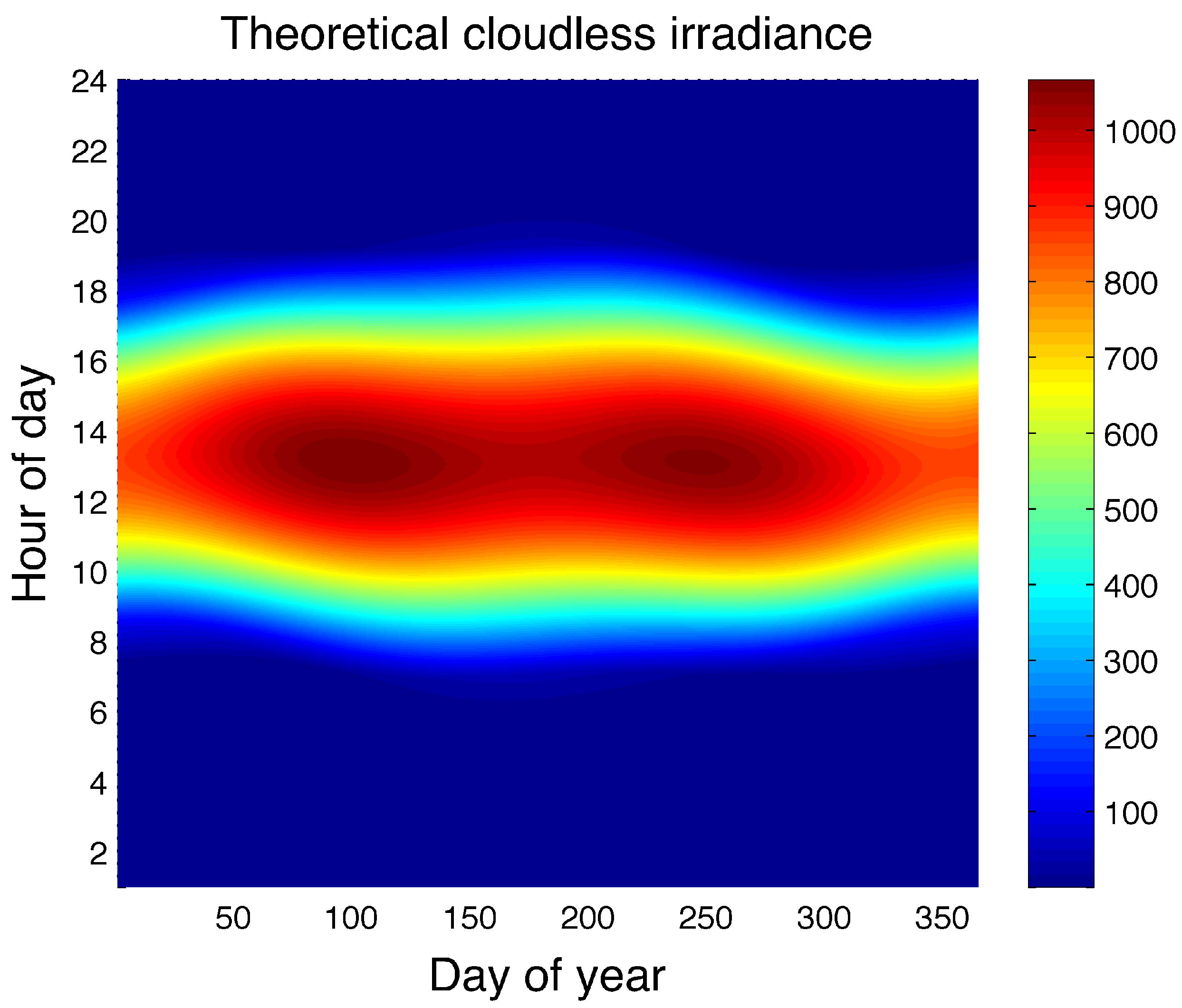
Using Equation (3), one can construct a map of the irradiance on a solar panel throughout the year. Figure 1 shows the yearly irradiance at a latitude of 30°, a tilt angle of 30°, and a reflectivity of $\rho =0.1$ and a altitude of 1.62 km.

Figure 1. Contour plot of irradiance $\frac{W}{m^2}$ as a function of day and time of day at a 30° tilt and a 30° latitude.

Figure 1. Contour plot of irradiance $\frac{W}{m^2}$ as a function of day and time of day at a 30° tilt and a 30° latitude.

If the total irradiance is integrated over a year using Equation (3), one can determine the angle at which the maximum energy is collected on a static solar panel. We assume that our solar panel is southward facing.

Taking the partial derivative of Equation (6) with respect to β and setting the equation to zero, one can derive the equation for the optimal angle,

$$cot\left(\beta \right)=\frac{\int \left(I_d+2I_{b}sin\left(\alpha \right)-\rho I_{t,h}\right)dt}{\int 2I_{b}cos\left(\alpha \right)cos(\gamma -A)dt}$$

(7)

which unfortunately involves integrals of transcendental functions. However, the graph of $cot\left(\beta \right)$ in conjunction with Equation (7) does allow us to conclude that an increase in ρ will increase the optimal angle β. We resort to numerical computations to determine the specific value of the optimal angle.

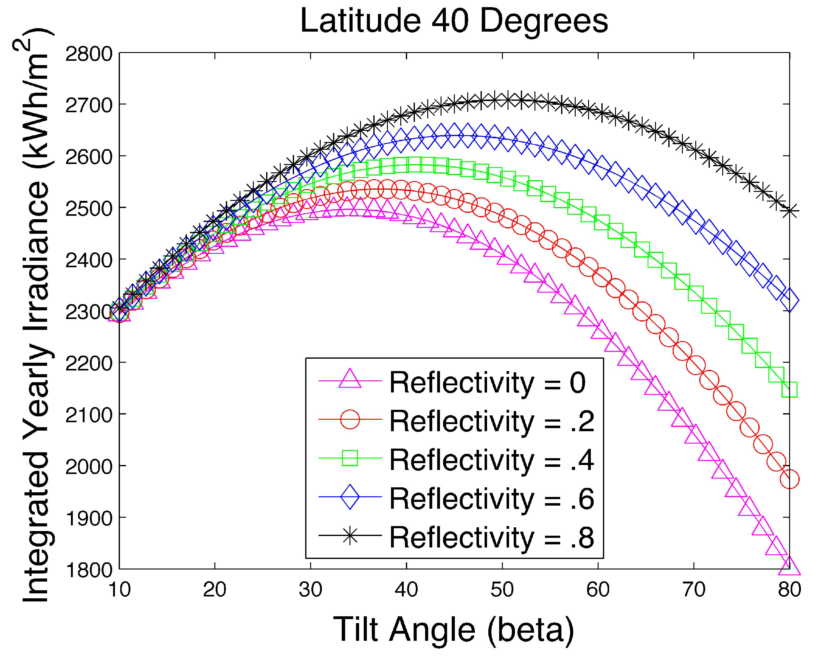
Figure 2 shows the integrated yearly irradiance as a function of the tilt angle at different reflectivities at a latitude of 40°. Table 3 shows the optimal angle and integrated annual energy per unit area at different reflectivities which can be extracted from Figure 2. The difference in the total integrated irradiance at the optimal angle is 1.9% between reflectivities of 0.2 and 0.4 and 4.1% between reflectivities of 0.2 and 0.6.

Figure 2. Integrated irradiance as a function of tilt angle and reflectance at 40° latitude.

Figure 2. Integrated irradiance as a function of tilt angle and reflectance at 40° latitude.

Table 3. Optimal angle vs. reflectivity for 40° latitude.

Reflectivity	Optimal Angle(β)	kWh/m2
0	$34.2^{°}$	2496
0.2	$37.3^{°}$	2536
0.4	$41.0^{°}$	2583
0.6	$45.3^{°}$	2639
0.8	$50.4^{°}$	2708

Table 3. Optimal angle vs. reflectivity for 40° latitude.

Reflectivity	Optimal Angle(β)	kWh/m2
0	$34.2^{°}$	2496
0.2	$37.3^{°}$	2536
0.4	$41.0^{°}$	2583
0.6	$45.3^{°}$	2639
0.8	$50.4^{°}$	2708

Since higher latitudes tend to accumulate snow in the winter, we perform a second study at a latitude of 40°. In the first part of the study, we maintain the reflectivity at 0.2 throughout the year. In the second part, we maintain the reflectivity at 0.2 in the summer months and 0.8 in the winter months for 180 days. The optimal angle for the first study is 37.3° with an annual yield of 2536 kWh/m². The optimal angle for the second study is 41° with an annual yield of 2581 kWh/m². The difference is only 1.8% in the annual yield at the different optimal angles. However, for comparison, we note that solar irradiation increases 4.1% if panel tilt angles are adjusted twice a year [7].

Table 4 shows the optimal angle and integrated annual energy at different reflectivities at a latitude of 30°. The difference in the total integrated irradiance at the optimal angle is 1.2% between reflectivities of 0.2 and 0.4 and 2.7% between reflectivities of 0.2 and 0.6.

Table 4. Optimal angle vs. reflectivity for 30° latitude.

Reflectivity	Optimal Angle(β)	kWh/m2
0	$26.1^{°}$	2628
0.2	$28.8^{°}$	2655
0.4	$32.0^{°}$	2688
0.6	$36.0^{°}$	2728
0.8	$40.8^{°}$	2779

Table 4. Optimal angle vs. reflectivity for 30° latitude.

Reflectivity	Optimal Angle(β)	kWh/m2
0	$26.1^{°}$	2628
0.2	$28.8^{°}$	2655
0.4	$32.0^{°}$	2688
0.6	$36.0^{°}$	2728
0.8	$40.8^{°}$	2779

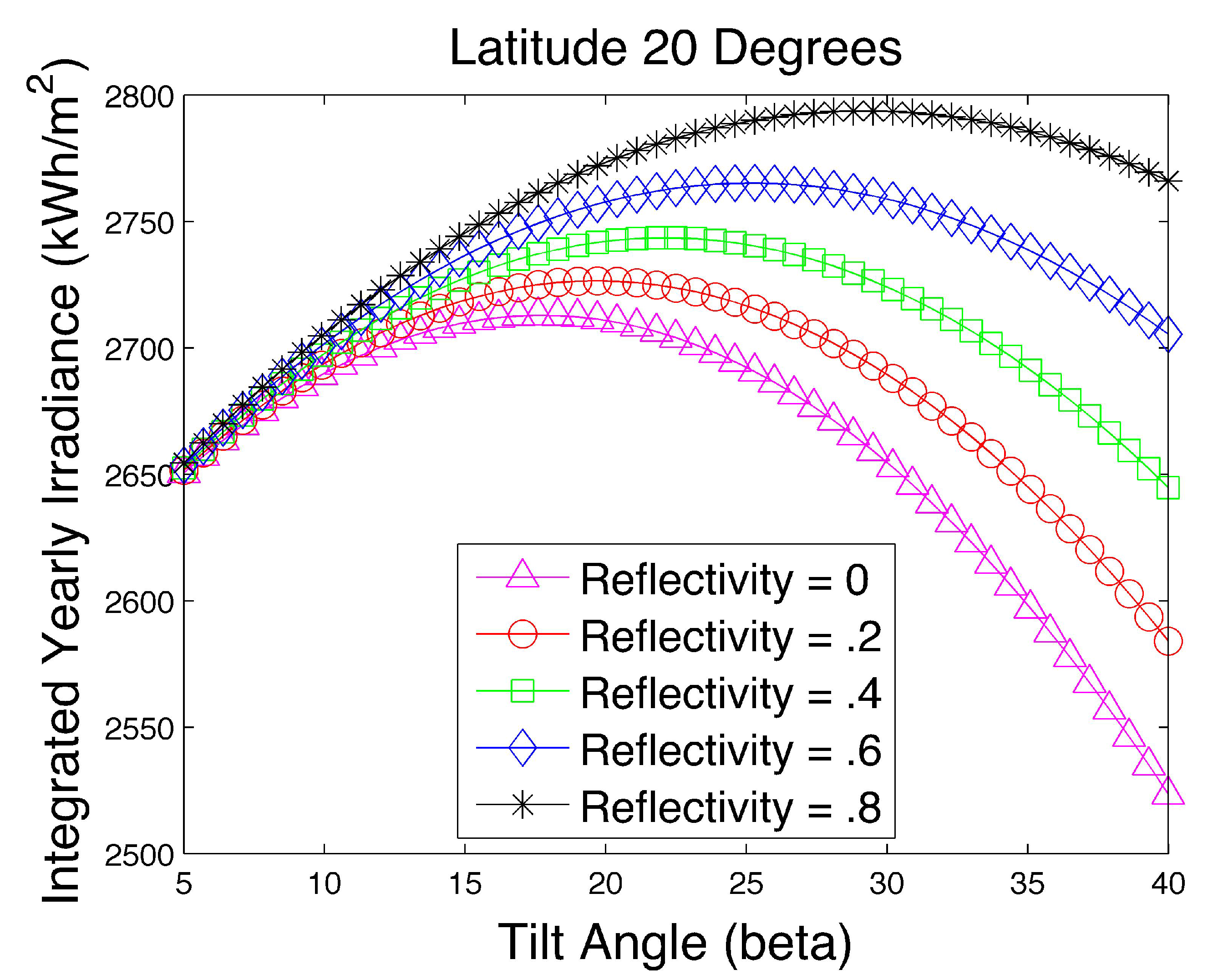
Figure 3 shows the integrated yearly irradiance as a function of the tilt angle at different reflectivities at a latitude of 20°. Note the difference in the vertical scale compared to Figure 2. Table 5 shows the optimal angle and integrated annual energy at different reflectivities at a latitude of 20°. The difference in the total integrated irradiance at the optimal angle is 0.6% between reflectivities of 0.2 and 0.4 and 1.4% between reflectivities of 0.2 and 0.6.

Figure 3. Integrated irradiance as a function of tilt angle and reflectance at 20° latitude.

Figure 3. Integrated irradiance as a function of tilt angle and reflectance at 20° latitude.

Table 5. Optimal angle vs. reflectivity for 20° latitude.

Reflectivity	Optimal Angle (β)	kWh/m2
0	$17.7^{°}$	2713
0.2	$19.7^{°}$	2727
0.4	$22.1^{°}$	2743
0.6	$25.2^{°}$	2765
0.8	$29.2^{°}$	2794

Table 5. Optimal angle vs. reflectivity for 20° latitude.

Reflectivity	Optimal Angle (β)	kWh/m2
0	$17.7^{°}$	2713
0.2	$19.7^{°}$	2727
0.4	$22.1^{°}$	2743
0.6	$25.2^{°}$	2765
0.8	$29.2^{°}$	2794

The maximum energy per unit area at the optimal angle is more sensitive to reflectivity at higher latitudes. At a latitude of 40°, a change of reflectivity between 0.2 to 0.6 can lead to a 4.1% increase in collected irradiation if the optimal angle is used. At a latitude of 20°, the gain is only 1.4%.

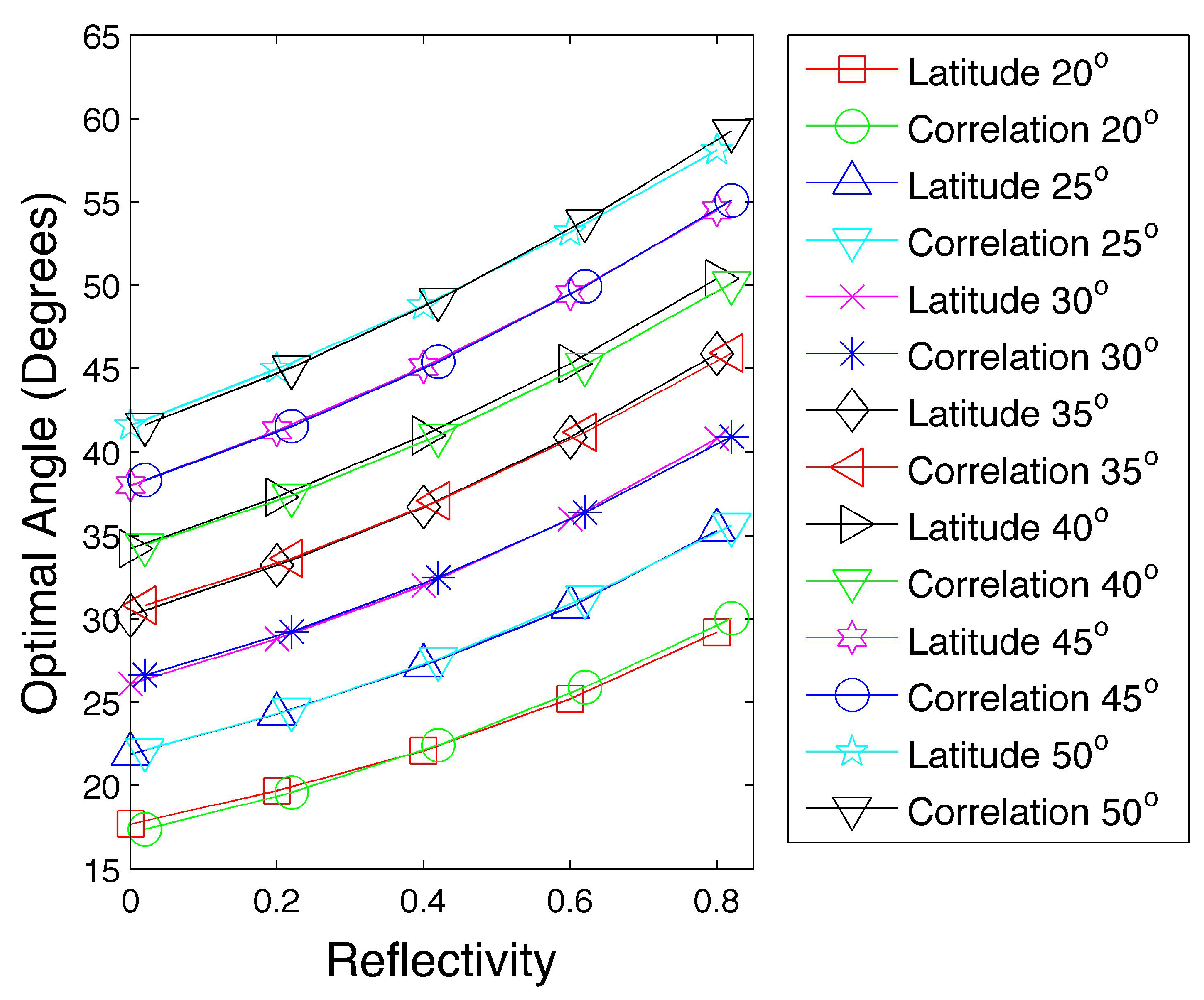
We summarize these results by plotting the optimal angle versus reflectivity and the maximum energy per unit area versus reflectivity at different latitudes. Using multiple regression, we design a correlation which allows the optimal angle (and maximum energy per unit area) to be computed based on reflectivity and latitude.

Figure 4 shows how the optimal angle changes with reflectivity at different latitudes. We plot both the data from the model and a quadratic multiple regression correlation for computing the optimal angle ${\beta }_{opt}$,

$${\beta }_{opt}=a+b\varphi +c\rho +d{\varphi }^2+e\varphi \rho +f{\rho }^2$$

(8)

where the latitude ϕ is in degrees and the coefficients $a,b,c,d,e$ and f are given in Table 6. We see that the correlation reproduces the model data well.

Figure 4. Optimal angle as a function of reflectivity and latitude.

Figure 4. Optimal angle as a function of reflectivity and latitude.

Table 6. Coefficients for multiple regression correlation for optimal angle.

a	b	c	d	e	f
–4.6230	1.2063	4.8992	–0.00574	0.20679	8.0612

Table 6. Coefficients for multiple regression correlation for optimal angle.

a	b	c	d	e	f
–4.6230	1.2063	4.8992	–0.00574	0.20679	8.0612

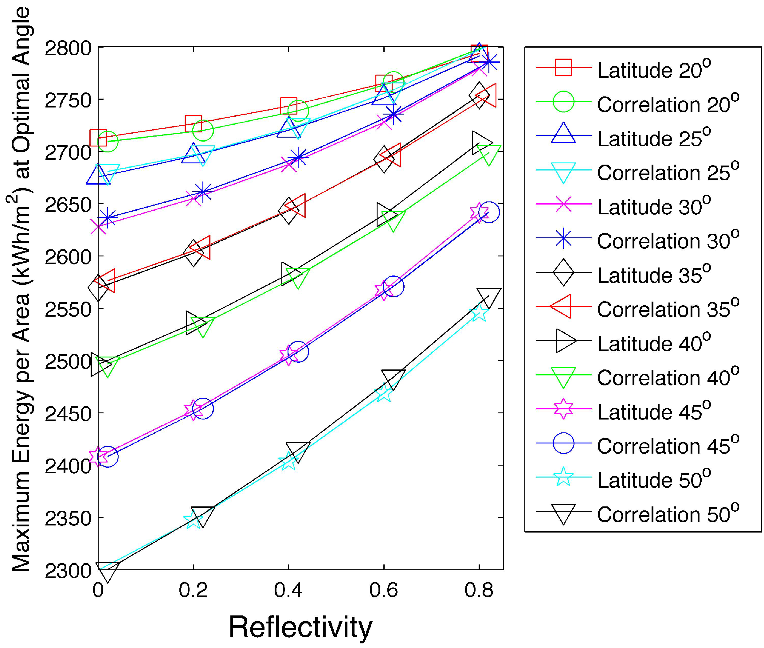
Figure 5 shows how the maximum energy per unit area changes at the optimal angle for different reflectivities at different latitudes. We plot both the data from the model and a multiple regression correlation for the maximum energy per unit area $E_{max}$ at the optimal angle,

$$E_{max}=\overline{a}+\overline{b}\varphi +\overline{c}\rho +\overline{d}{\varphi }^2+\overline{e}\varphi \rho +\overline{f}{\rho }^2$$

(9)

where ϕ is in degrees and the coefficients $\overline{a},\overline{b},\overline{c},\overline{d},\overline{e}$ and $\overline{f}$ are given in Table 7. Again we see that the correlation reproduces the model data well.

Figure 5. Maximum energy per unit area at optimal angle as a function of reflectivity and latitude.

Figure 5. Maximum energy per unit area at optimal angle as a function of reflectivity and latitude.

Table 7. Coefficients for multiple regression correlation for maximum energy per unit area at optimal angle.

$\overline{a}$	$\overline{b}$	$\overline{c}$	$\overline{d}$	$\overline{e}$	$\overline{f}$
2666.94	8.4470	–113.25	–0.31756	7.0728	103.85

Table 7. Coefficients for multiple regression correlation for maximum energy per unit area at optimal angle.

$\overline{a}$	$\overline{b}$	$\overline{c}$	$\overline{d}$	$\overline{e}$	$\overline{f}$
2666.94	8.4470	–113.25	–0.31756	7.0728	103.85

While the optimal angle spans approximately the same range as the reflectivity varies at different latitudes (Figure 4), the maximum energy per unit area in Figure 5 does not. The range of maximum energy per unit area at different reflectivities is less at lower latitudes and more at higher latitudes. Energy gathered from solar panels at higher latitudes is more sensitive to the optimal tilt angle than at lower latitudes in regards to variations in reflectivity.

4. The Influence of Cloud Cover on the Optimal Tilt Angle

Despite the fact that Albuquerque, New Mexico is located in an area with a high average annual irradiance [22], there is considerable day to day variability. We determine that the coefficient of variation is highest during the winter months of the period of study from December 2012 to November 2013. Optimizing the tilt angle for cloud cover depends on identifying statistically reliable predictions of cloud cover. Months with low cloud cover and low variations in cloud cover would potentially be more important in optimizing a panel tilt angle.

4.1. Power Variability at PNM Prosperity Site

The PNM Prosperity Energy Storage project is the nation’s first solar storage facility that is fully integrated into a utility’s power grid. The project features one of the largest facilities which combines battery storage and photovoltaic energy in the nation. The size of the site is approximately 4.9 acres. The array is composed of 2158 panels which produce up to 500 kilowatts and are maintained at a tilt angle of 25°. Since the tilt angle 25° is less than the latitude 35°, solar collection is biased to optimizing energy in the summer months when electricity is in higher demand. Prosperity is shown in Figure 6a. The data acquisition system includes sensors that capture (among other variables) irradiance, power and temperature. While the site sampling rate is 30 samples per second, we only use 2 samples per hour or 48 samples per day of power readings for our analysis. Our study starts on 1 December 2012, and ends on 30 November 2013. Figure 6b shows the power signal of an arbitrary day, 1 November 2013.

Figure 6. (a) Aerial view of Prosperity. The upper left corner shows a closer view of the panel array; (b) Power signal generated by Prosperity on 1 November 2013.

Figure 6. (a) Aerial view of Prosperity. The upper left corner shows a closer view of the panel array; (b) Power signal generated by Prosperity on 1 November 2013.

Figure 7. Energy production, May 2013 and November 2013.

Figure 7. Energy production, May 2013 and November 2013.

Let $E_d$ be the energy collected in a day d

$$E_d=\int P_d\left(t\right)dt,$$

(10)

where $P_d\left(t\right)$ is the power signal in day d. Equation (10) can be approximated by

$$E_d\approx \sum _{n=0}^{47}{P}_d\left(n\right)\Delta t,$$

(11)

where $P_d\left(n\right)$ is the power signal at sampling time n and $\Delta t=\frac{1}{2}$ is the sampling interval, in hours. Figure 7 shows the daily energy production for two contrasting months in Megawatt hours (MWh): May 2013 and November 2013. While the first is a high energy producing month, the latter is characterized by lower production due to the season and weather conditions (e.g., snow days 20–23). The daily energy production in the months of November and May is quite variable even in Albuquerque, a city with approximately 300 days of sunshine.

Let $\overline{E_m}$ denote the average energy production of month $m\in \{Jan,Feb,...,Dec\}$ and $D_m$ be the number of days in the month. Furthermore, let $c{v}_m$ denote the daily coefficient of variation of the energy production over a month $m\in \{Jan,Feb,...,Dec\}$ computed using

$$c{v}_m=\frac{1}{\overline{E_m}}\sqrt{\frac{{\sum }_{d=1}^{D_m}{(E_d-\overline{E_m})}^2}{D_m-1}}.$$

(12)

Figure 8a shows the average energy production per month and Figure 8b the coefficient of variation. During the summer season (June, July, August), the daily energy production is above 2.4 MWh and the coefficient of variability is below 20%. In contrast, during the months of November, December and January, the daily energy production is below 2 MWh and the coefficient of variability is relatively high (above 30%). Wilcox [13] shows that the monthly coefficient of variation for New Mexico is highest in February based on eight years of data from 1998–2005.

Figure 8. (a) Average energy production, December 2012–November 2013; and (b) corresponding coefficient of variation.

Figure 8. (a) Average energy production, December 2012–November 2013; and (b) corresponding coefficient of variation.

4.2. Sensitivity to Cloud Cover at Prosperity 35° Latitude

A careful study of weather and its effect on the optimal tilt angle would account for weather patterns and variability over multiple years. Here we perform a sensitivity study to determine how much the optimal tilt angle is affected by cloud cover at a ground reflectivity of 0.2. WeatherSpark [23] presents average cloud cover from historical records from 1974 to 2012 in Albuquerque, New Mexico based on data from the National Oceanic and Atmospheric Administration. Their data shows that the smallest variation in cloud cover occurs in June, July, August and September. We use the site’s median cloud cover and percentile bands to estimate the average cloud cover and standard deviation throughout the year. The cloud cover is used in our model by reducing the irradiance by the fraction of cloud cover. Cloud cover is made stochastic by daily sampling from a normal distribution whose mean and standard deviation are determined from WeatherSpark’s data. Figure 9 shows the variation in the fraction of cloud cover used in two of our model simulations over the course of a year. For our calculations, we use a standard deviation in cloud cover (6.7%–10.7% depending on the month) that is small compared to what would be used based on WeatherSpark’s percentile bands.

Figure 9. Simulated cloud cover based on historical data from 1974-2012.

Figure 9. Simulated cloud cover based on historical data from 1974-2012.

Table 8 presents the optimal angle, the energy per unit area at the optimal angle, and the energy per unit area at the optimal cloudless angle (33.2°) for five (out of ten) simulations which account for cloud cover at a latitude of 35°. Cloud cover significantly reduces the integrated annual irradiance from a cloudless value of 2603 kWh/m² to a range from 1581 to 1607 kWh/m². However, there is little difference in the optimal angles 34.2°–34.6° in the ten simulations. Moreover, the optimal cloudless angle (33.2°) fares well in producing the near optimal energy over the cloudy year compared to the optimal angles which account for cloud cover. The difference between the integrated yearly irradiance (kWh/m²) at the optimal angle (considering cloud angle) and the integrated yearly irradiance at the optimal cloudless angle is less than 0.03% in all ten simulations.

Table 8. Optimal angle and annual energy per unit area in stochastic cloud cover model.

Simulation	Optimal Angle(β)	kWh/m2 at Optimal Angle	kWh/m2 at Optimal Cloudless Angle $33.2^{°}$
Simulation 1	$34.4^{°}$	1606.6	1606.3
Simulation 2	$34.6^{°}$	1598.2	1597.9
Simulation 3	$34.4^{°}$	1607.1	1606.8
Simulation 4	$34.4^{°}$	1581.8	1581.5
Simulation 5	$34.4^{°}$	1601.9	1601.6

Table 8. Optimal angle and annual energy per unit area in stochastic cloud cover model.

Simulation	Optimal Angle(β)	kWh/m2 at Optimal Angle	kWh/m2 at Optimal Cloudless Angle $33.2^{°}$
Simulation 1	$34.4^{°}$	1606.6	1606.3
Simulation 2	$34.6^{°}$	1598.2	1597.9
Simulation 3	$34.4^{°}$	1607.1	1606.8
Simulation 4	$34.4^{°}$	1581.8	1581.5
Simulation 5	$34.4^{°}$	1601.9	1601.6

Thus our model only predicts small changes in optimal tilt angle when cloud cover is considered. The variations in optimal tilt angle described by Lave [6] may be driven by multiple factors (e.g., topography) including weather.

5. Conclusions

The influence of ground reflectivity on the optimal tilt angle of solar panels is determined by numerically integrating the total irradiance over a year. The total irradiance is composed of direct beam, diffuse and reflected components. While the influence of reflectivity is minimal at lower elevations, it does become slightly more important at higher latitudes (e.g., 40°). Optimizing the angle for reflectivities of 0.2 in the summer and 0.8 in the winter (assuming snow cover) can improve the integrated irradiance by 1.8% at a 40° latitude. We also develop a correlation which computes the optimal angle and maximum energy as a function of reflectivity and latitude.

Subsequently we evaluate the sensitivity of the optimal angle to cloud cover at a latitude of 35°. Our model shows that while the total integrated irradiance is significantly reduced compared to a cloudless year, the optimal angle (which accounts for cloud cover) and its associated integrated irradiance deviates little from the optimal cloudless angle and its integrated irradiance. Our computations show a deviation of only 1.5° from the cloudless optimal angle of 33.2° for ten stochastic simulations which incorporate historical data from Weatherspark [23].

References

1. Lewis, G. Optimum Tilt of Solar Collector. Sol. Wind Energy 1987, 4, 407–410. [Google Scholar] [CrossRef]
2. Duffie, J.A.; Beckman, W.A. Solar Engineering of Thermal Processes; Wiley: New York, NY, USA, 1980. [Google Scholar]
3. Calabrò, E. An Algorithm to Determine the Optimum Tilt Angle of a Solar Panel from Global Horizontal Solar Radiation. J. Renew. Energy 2013, 1. [Google Scholar] [CrossRef]
4. Idowu, O.S.; Olarenwaju, O.M.; Ifedayo, O.I. Determination of Optimum Tilt Angles for Collectors in Low-Latitude Tropical Regions. Int. J. Energy Environ. Eng. 2013, 4. [Google Scholar] [CrossRef]
5. Darhmaoui, H.; Lahjouji, D. Latitude Based Model for Tilt Angle Optimization for Collectors in the Mediterranean Region. Energy Procedia 2013, 42, 426–435. [Google Scholar] [CrossRef]
6. Lave, M.; Kleissl, J. Optimum Fixed Orientations and Benefits of Tracking for Capturing Solar Radiation in the Continental United States. Renew. Energy 2011, 36, 1145–1152. [Google Scholar] [CrossRef]
7. Landau, C.R. Optimum Tilt of Solar Panels. Available online: www.solarpaneltilt.com (accessed on 29 June 2015).
8. Ineichen, P.; Perez, R.; Seals, R. The Importance of Correct Albedo Determination for Adequately Modeling Energy Received by Tilted Surfaces. Sol. Energy 1987, 39, 301–305. [Google Scholar] [CrossRef]
9. Kambezidis, H.D.; Psiloglou, B.E.; Gueymard, C. Measurements and Models for Total Solar Irradiance on Inclined Surface in Athens, Greece. Sol. Energy 1994, 53, 177–185. [Google Scholar] [CrossRef]
10. Kotak, Y.; Gul, M.S.; Muneer, T.; Ivanova, S.M. Invesigating the Impact of Ground Albedo on the Performance of PV Systems. In Proceedings of CIBSE Technical Symposium, London, UK, 16–17 April 2015.
11. Christensen, C.B.; Barker, G.M. Effects of Tilt and Azimuth on Annual Incident Solar Radiation for United States Locations. In Proceedings of Solar Forum 2001: Solar Energy: The Power to Choose, Washington, DC, USA, 21–25 April 2001.
12. Liu, B.Y.H.; Jordan, R.C. The Long Term Average Performance of Solar Collectors. Sol. Energy 1963, 7, 53–74. [Google Scholar] [CrossRef]
13. Wilcox, S.; Gueymard, C.A. Spatial and Temporal Variability of the Solar Resource in the United States. In Proceedings of the ASES Solar 2010, Phoeniz, AZ, USA, 17–22 May 2010.
14. PNM Prosperity Energy Storage Project. Available online: https://share.pnmresources.com/Public/Pages/default.aspx (accessed on 29 June 2015).
15. Stine, W.B.; Geyer, M. Power from the Sun. Chapters 3 and 4. Available online: www.powerfromthesun.net/book.html (accessed on 29 June 2015).
16. Bird, R.E.; Hulstrom, R.L. Simplified Clear Sky Model for Direct and Diffuse Insolation on Horizontal Surfaces; Technical Report No. SERI/TR-642-761; Solar Energy Research Institute: Golden, CO, USA, 1981. [Google Scholar]
17. Bird Clear Sky Model. Available online: http://rredc.nrel.gov/solar/models/clearsky (accessed on 29 June 2015).
18. Hottel, H.C. A Simple Model for Estimating the Transmittance of Direct Solar Radiation through Clear Atmospheres. Sol. Energy 1976, 18, 129–134. [Google Scholar] [CrossRef]
19. Markvart, T.; Castaner, L. Practical Handbook of Photovoltaics, Fundamentals and Applications; Elsevier: New York, NY, USA, 2003. [Google Scholar]
20. Coakley, J.A. Reflectance and Albedo, Surface. In Encyclopeida of the Atmospheric Sciences; Holton, J.R., Curry, J.A., Pyle, J.A., Eds.; Academic Press: Waltham, MA, USA, 2002; pp. 1914–1923. [Google Scholar]
21. Chang, T.P. The Sun’s Apparent Position and the Optimal Tilt Angle of a Solar Collector in the Northern Hemisphere. Sol. Energy 2009, 83, 1274–1284. [Google Scholar] [CrossRef]
22. National Renewable Energy Laboratory. Available online: www.nrel.gov/gis/solar.html (accessed on 30 June 2015).
23. Average Weather For Albuquerque, New Mexico, USA. Available online: https://weatherspark.com/averages/29561/Albuquerque-New-Mexico-United-States (accessed on 16 September 2015).