Modeling and Analysis of a Low-Voltage DC Distribution System

Abstract

It is well known that the Low-Voltage DC (LVDC) distribution system is a promising topology as a future smart distribution system due to its high efficiency and reliability. However, there are still some challenges in the construction and implementation of an LVDC system. For practical application of the LVDC system, therefore, it is necessary to perform any simulation in advance by considering various conditions that can occur in an LVDC system. In order to provide a foundation for analyzing a DC system, this paper presents an LVDC distribution system model including essential components such as power electronic devices, Distributed Energy Resource (DER), and Energy Storage System (ESS), which can be considered for implementation in an LVDC system using Electro-Magnetic Transient Program (EMTP) software. Moreover, an analysis of the characteristic in both the steady state and the transient state is conducted in an LVDC distribution system.

1. Introduction

Recently, new DC power distribution systems have been researched and developed due to various advantages, such as higher efficiency and reliability, fewer conversion stages, and uninterrupted power delivery compared to conventional AC systems [1,2,3]. Furthermore, renewable resource systems, such as photovoltaic power generation, wind power generation, and electric vehicles are considered to be good alternatives in electric power systems. These distributed resources and electric vehicles generate and use DC voltage, so they must interface with DC distribution systems, which are more efficient than the existing AC distribution systems when dealing with DC-based sources and devices. Due to these advantages, it is expected that the installation of DC systems in housing complexes, buildings, etc. will increase. For this reason, the demand for applications of DC systems has increased [4,5].

In past years, many studies of DC networks have reviewed the detailed aspects of DC distribution systems. The development of the Low-Voltage DC (LVDC) network was started 2005 in Finland as a continuum to the development of 1kV intermediate LVDC distribution systems [6]. In [7], the possibility of the adoption of DC sources in low- and medium-voltage networks was evaluated. It has been shown that if the losses in converters due to the conversion stage can be significantly reduced by applying an LVDC system, the total system losses will be decreased compared to those of the conventional AC network. The feasibility of an LVDC network for use in commercial facilities was studied in [8]. This study concludes that the most suitable DC voltage level is between 300 and 400 from both the technical and economical points of view, and that the implementation of an LVDC distribution system is more beneficial than an AC system. At Lappeenranta University, various studies have been performed in real test bed systems. The realistic concept of an LVDC distribution system, including the grounding method and fault analysis, is presented in [6] and [9]. LVDC network concepts with somewhat similar properties and some of the same objectives have been introduced in [8,10,11].

Although there are detailed reviews and analyses considering various aspects of LVDC systems in the aforementioned studies, there are still some challenges, such as the simulation and implementation of DC systems because of a lack of object models and simulation skill. To provide a foundation for analyzing the diverse characteristics of LVDC network systems, this paper proposes an LVDC system that includes essential components such as power electronic devices, DER, and ESS, which can be considered when implementing LVDC distribution systems. Moreover, an analysis of the steady state and transient characteristics are conducted. In Section 2, the essential elements of the LVDC distribution system are modeled using the EMTP software. The modeled components are implemented using EMTP/MODELS, which is a symbolic language interpreter for EMTP. In Section 3, an analysis of the steady-state characteristics of an LVDC distribution system, such as load unbalance and the connection of a photovoltaic (PV) generation system as a DER, is presented. In Section 4, an analysis of the transient state in an LVDC distribution system, considering line faults and series arc faults, is presented. Finally, the conclusion derived from our study is discussed in Section 5.

2. Modeling of Components in LVDC Distribution System

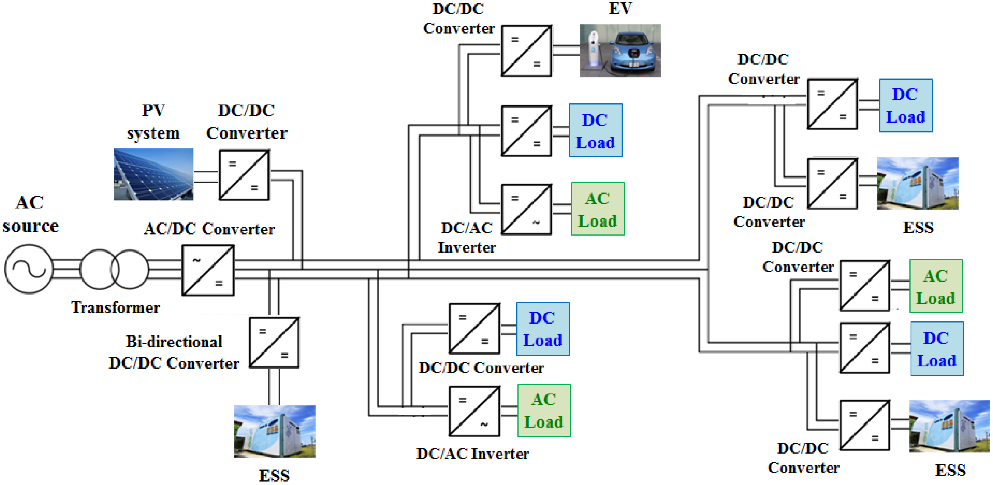
Figure 1 shows the concept of an LVDC distribution system. Unlike a conventional AC system, an LVDC system needs power electronic devices. In addition, the distributed generation, ESS, and various types of load are connected to the main DC system through the power electronic devices. In this section, therefore, the modeling of the power electronic device, distribution line, load, PV system, and ESS, which are essential elements of an LVDC distribution system, is conducted based on a system such as that in Figure 1.

Figure 1. Concept of an LVDC distribution system.

Figure 1. Concept of an LVDC distribution system.

2.1. Power Electronic Device Modeling

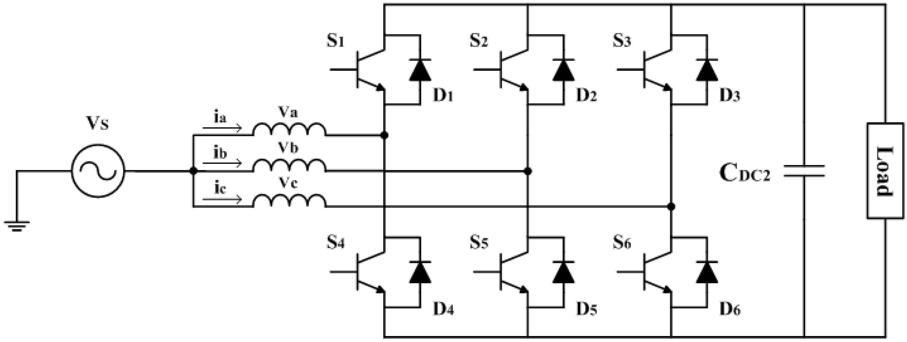
2.1.1. AC/DC Converter

An AC/DC Converter converts AC voltage and current to DC voltage and current, respectively. The basic circuit diagram of a three-phase AC/DC converter is shown in Figure 2. In this study, the AC/DC converter is modeled using the Sinusoidal Pulse Width Modulation (SPWM) control scheme.

Figure 2. Circuit diagram of a three-phase AC/DC converter.

Figure 2. Circuit diagram of a three-phase AC/DC converter.

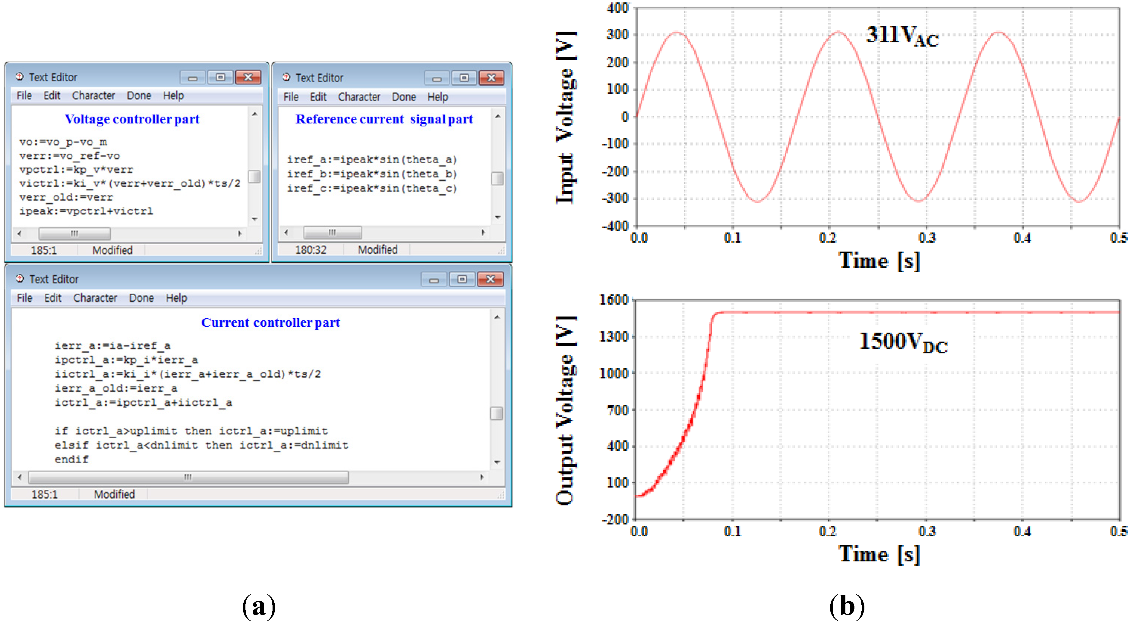
In this converter, the three reference currents are obtained by multiplying the three-phase sinusoidal balanced voltage with a gain G, which represents the smoothed output of a Proportional-Integral (PI) controller used for obtaining a null steady-state error of the DC voltage [12]. To control the switches in the converter circuit, some parts of the EMTP/MODELS source code are shown in Figure 3a. The voltage controller generates the peak value of the reference current by comparing the output voltage and its reference value. Then, in reference current signal generating parts, the reference value of the input current is generated in phase with the input voltage. Finally, the current controller generates the control signal of the input current of each phase by comparing the input current and its reference value [13]. Figure 3b shows the input and output voltage of the AC/DC converter. From the result, we can see that the modeled AC/DC converter can properly convert AC voltage to DC voltage. Therefore, this converter model can be applied to LVDC system for the purpose of converting AC source into DC.

Figure 3. (a) EMTP/MODELS code for modeling an AC/DC converter; (b) Input voltage and output voltage of the modeled AC/DC converter.

Figure 3. (a) EMTP/MODELS code for modeling an AC/DC converter; (b) Input voltage and output voltage of the modeled AC/DC converter.

2.1.2. DC/DC Converter

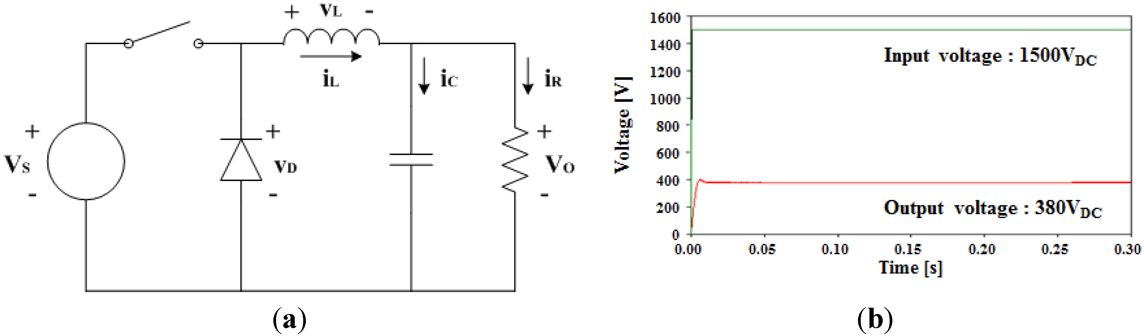
A DC/DC converter can increase or decrease the magnitude of a DC voltage. A DC/DC buck converter is used to generate a lower output voltage from a higher DC input voltage [14]. That is, a DC/DC buck converter can be used to step down the high voltage level of the main distribution line to the low voltage level required by the end customer. Figure 4 shows the basic circuit and the output voltage of the DC/DC buck converter modeled in this study using EMTP. As shown in Figure 4b, the modeled DC/DC buck converter is accurately operated to step down the higher input voltage to lower output voltage as designed.

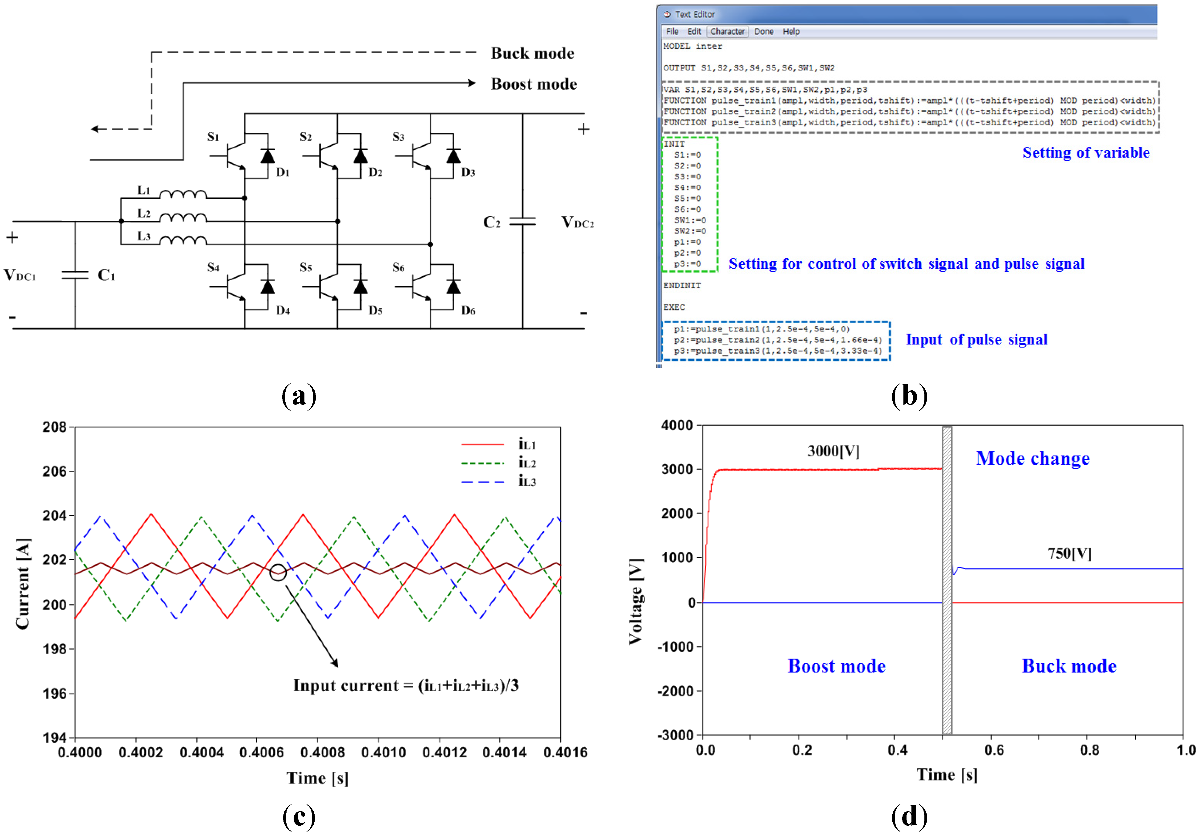
A bi-directional DC/DC converter is also modeled and it can be used to interconnect the main power system and various renewable resources, such as a PV power generation or ESS. In this paper, a bi-directional DC/DC converter, for which the magnitude of the output voltage is controlled by a three-phase interleaved method, is modeled. In the interleaved method, a converter conducts a switching operation with a time difference according to the number of phases [15,16]. This method is effective for reducing the ripple of the input current, as shown in Figure 5c. In order to model the bi-directional DC/DC converter based on the interleaved method, we use EMTP/MODELS to conduct total converter control including the time difference and mode change in boost and buck modes. In Figure 5c, a switching operation with a time difference is accurately conducted so that the ripple of input current is effectively reduced. Also, the output voltage is properly controlled through a modeled bi-directional DC/DC converter according to the mode change as shown in Figure 5d. From the verification of the performance of a modeled bi-directional DC/DC converter, we can conclude that a modeled bi-directional DC/DC converter can be used for interconnecting the LVDC system with renewable resources that generate DC voltage.

Figure 4. (a) Circuit diagram of DC/DC buck converter; and (b) Input voltage and output voltage of the modeled DC/DC Buck converter.

Figure 4. (a) Circuit diagram of DC/DC buck converter; and (b) Input voltage and output voltage of the modeled DC/DC Buck converter.

Figure 5. (a) Circuit diagram of a bi-directional DC/DC converter; (b) EMTP/MODELS code of the interleaved method; (c) Reduction in ripple of input current by application of the interleaved method; and (d) Output voltage of a bi-directional DC/DC buck converter.

Figure 5. (a) Circuit diagram of a bi-directional DC/DC converter; (b) EMTP/MODELS code of the interleaved method; (c) Reduction in ripple of input current by application of the interleaved method; and (d) Output voltage of a bi-directional DC/DC buck converter.

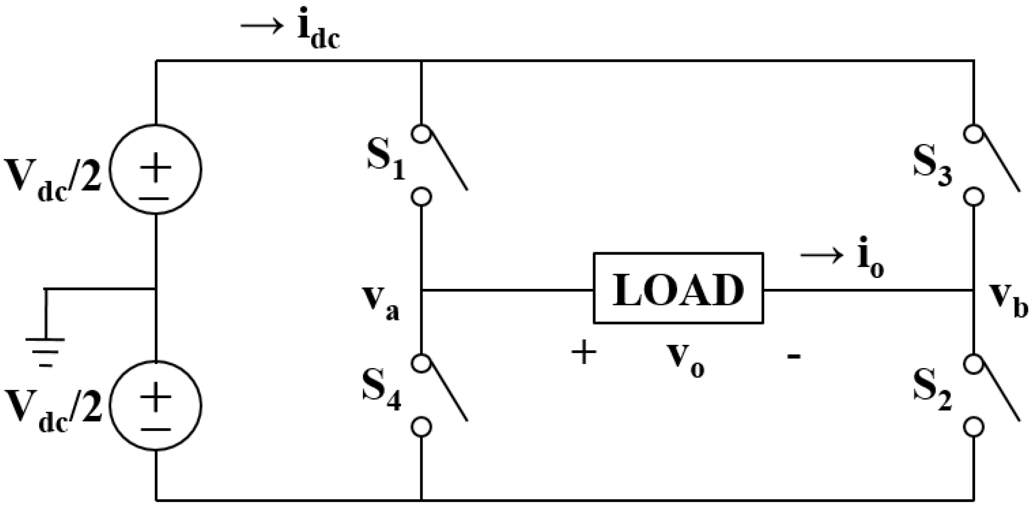
2.1.3. DC/AC Inverter

The inverter converts the voltage or current from DC to AC with variable amplitudes and frequencies. Figure 6 shows a circuit of a single-phase full bridge inverter with two ideal input voltage sources and four switches.

Figure 6. Single-phase full-bridge inverter circuit.

Figure 6. Single-phase full-bridge inverter circuit.

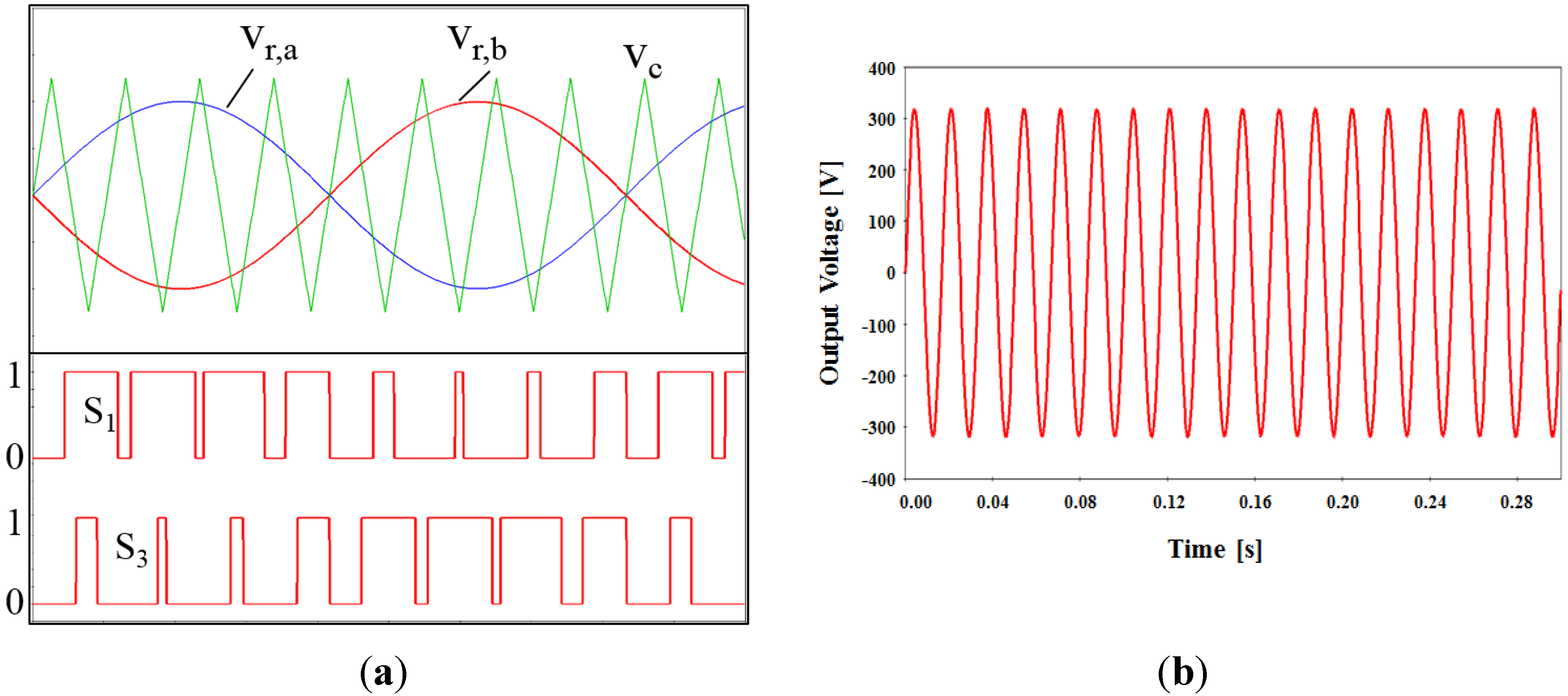
In this study, the SPWM control technique, which is one of the PWM methods, is applied to operate the switches shown in Figure 7a. In the SPWM method, the switches are operated by comparing the magnitude of the sinusoidal wave with that of the triangle wave [14,17]. To control the output voltage, the SPWM method has two indexes: the amplitude modulation index (ma) and frequency modulation index (mf). The ma, which is the ratio of the peak of the sinusoidal wave to that of the triangle wave, controls the amplitude of the output voltage, and the mf, which is the ratio of the frequency of the triangle wave to that of the sinusoidal wave, can adjust the harmonics. Figure 7b shows the output voltage waveform of the SPWM inverter. In Figure 7b, the output voltage of the modeled inverter has peak value as about 311V and we can find that the conversion of voltage from DC to AC is properly conducted. Thus, the modeled inverter is worked as ideal AC source so that it can be used to supply the AC power to AC loads in LVDC distribution system.

Figure 7. (a) The operation of switches according to the SPWM method; and (b) Output voltage waveform of the SPWM inverter.

Figure 7. (a) The operation of switches according to the SPWM method; and (b) Output voltage waveform of the SPWM inverter.

2.2. Distribution Line Modeling

In order to construct an LVDC distribution system, we consider which line models are acceptable for this system. Currently, there is no restriction on applying conventional lines to a DC system at low voltage levels according to research from the SFS (Finnish Standards Association) standard [18,19]. The research of KETI (Korea Electronics Technology Institute) also concluded that there is no efficiency problem when applying conventional lines to a DC system [20]. In this paper, therefore, conventional line data in an AC system is used to model the line for a DC system.

2.2.1. Overhead Distribution Line

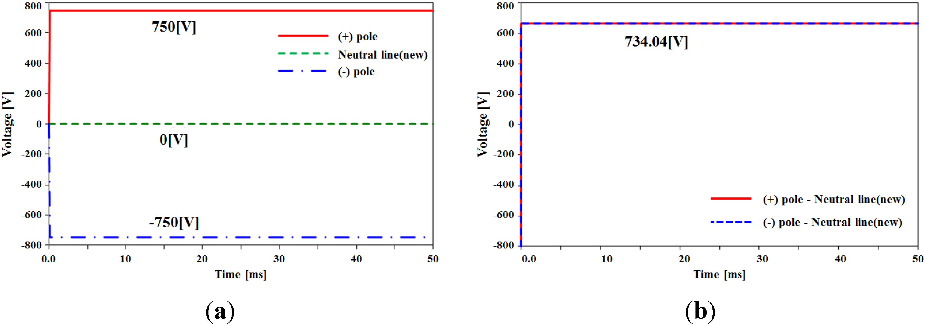
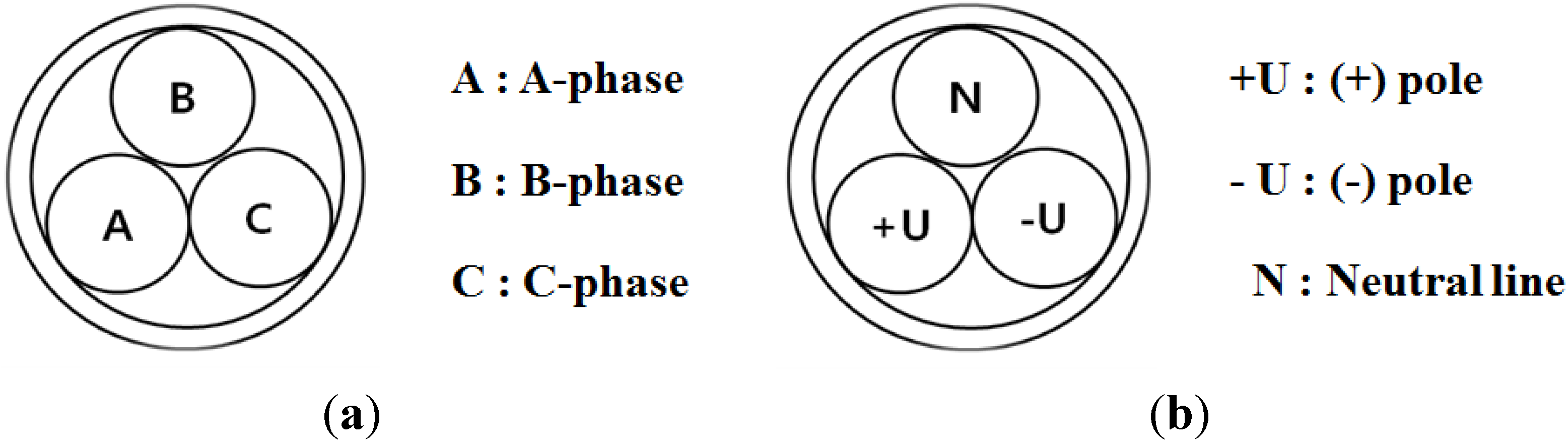
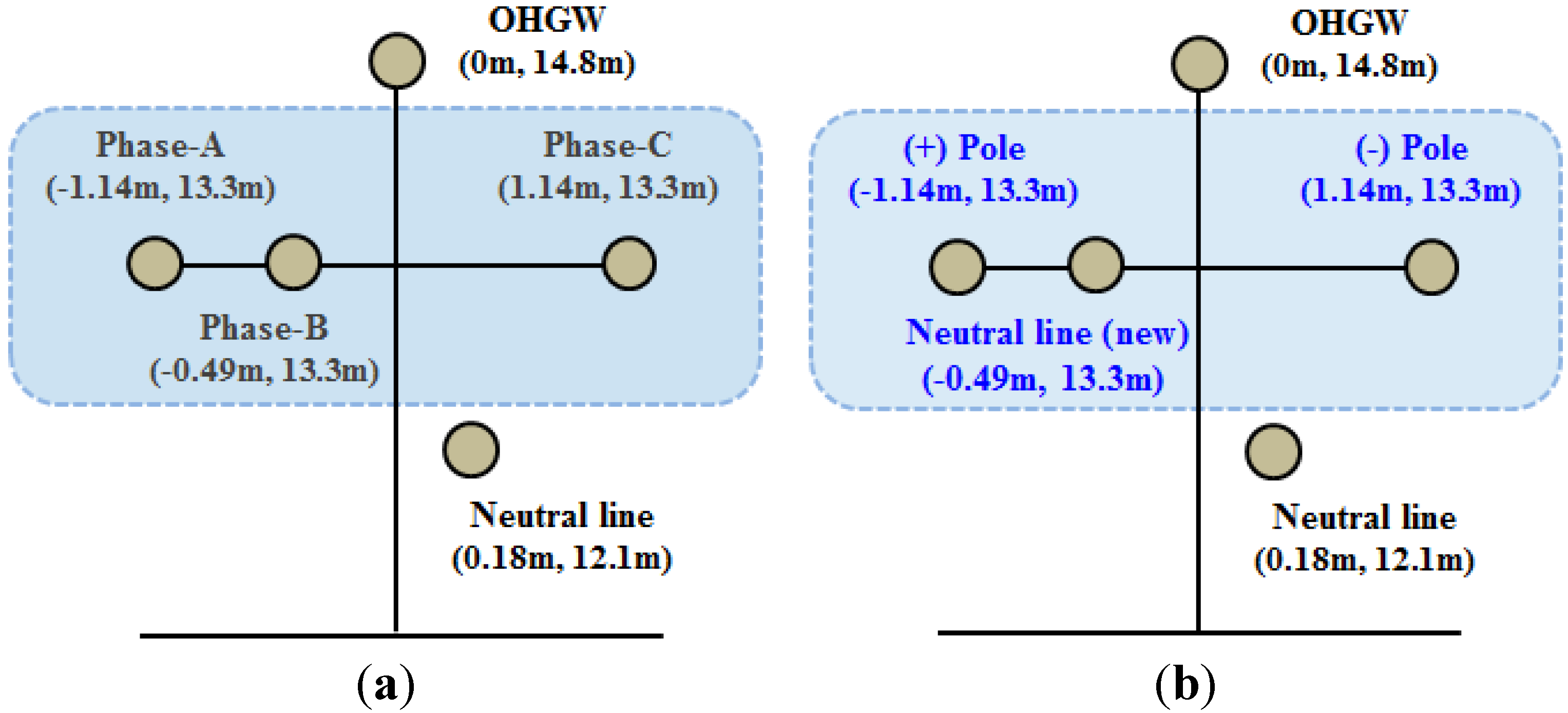
Figure 8 shows the concept of overhead distribution line when the conventional AC system is converted into DC system. As shown in Figure 8a,b, the existing A-phase, B-phase, and C-phase can be replaced with (+) pole, neutral line (new), and (−) pole, respectively.

Figure 8. (a) Configuration of overhead distribution line of conventional AC system; and (b) Configuration of overhead distribution line of DC system.

Figure 8. (a) Configuration of overhead distribution line of conventional AC system; and (b) Configuration of overhead distribution line of DC system.

The type of overhead distribution line is made of Outdoor Weather Proof PVC Insulated Wire (OW) 100 mm², and the detailed parameters about modeled line are presented in Table 1.

Table 1. Parameters of modeled line.

Dimension (mm2)	Outer Diameter (mm)	Total Cable Diameter(mm)	Conductor Resistance (Ω/km)
100	13.0	16.0	0.185

Table 1. Parameters of modeled line.

Dimension (mm2)	Outer Diameter (mm)	Total Cable Diameter(mm)	Conductor Resistance (Ω/km)
100	13.0	16.0	0.185

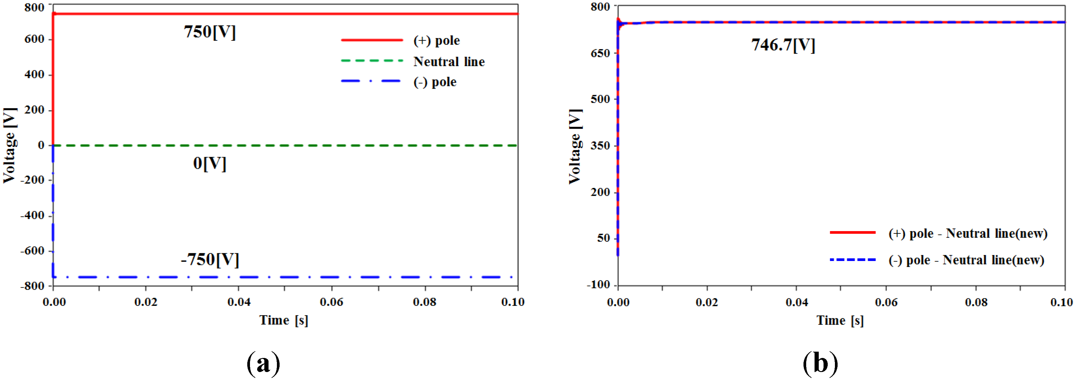
Based on the Figure 8 and Table 1, the overhead distribution line is modeled by using EMTP/LCC component. The physical data for modeling the line, such as the geographical position of the conductor and line parameters, can be input through LCC component. Figure 9a,b shows the source voltage and distribution line voltage, respectively. Although the voltage drop is occurred due to line impedance, we can find that the conventional line of AC system can be normally applied to DC system.

Figure 9. (a) Source voltage; (b) Modeled distribution line voltage.

Figure 9. (a) Source voltage; (b) Modeled distribution line voltage.

2.2.2. Underground Cable

Based on the some reference which introduce the possibility about use of the current underground cable [18,19], Figure 10 describes the configuration of underground cable when converting the conventional AC system into DC system. As shown in Figure 10a,b, the existing A-phase, B-phase, and C-phase can be replaced with (+) pole, neutral line, and (−) pole.

Figure 10. (a) Configuration of underground cable of conventional AC system; and (b) Configuration of underground cable of DC system.

Figure 10. (a) Configuration of underground cable of conventional AC system; and (b) Configuration of underground cable of DC system.

The type of underground cable is made of cross-linked polyethylene vinyl sheath (CV) 240 mm². The detailed parameters about modeled underground cable are presented in Table 2.

Table 2. Parameters of modeled underground cable.

Dimension (mm2)	Core diameter (mm)	Sheath layer(mm)	Conductor resistance (Ω/km)
240	18.3	2.6	0.0754

Table 2. Parameters of modeled underground cable.

Dimension (mm2)	Core diameter (mm)	Sheath layer(mm)	Conductor resistance (Ω/km)
240	18.3	2.6	0.0754

Based on the Figure 10 and Table 2, the underground cable is modeled using LCC component in common with the overhead distribution line. The physical data and line parameters about the underground cable are input through LCC component. Figure 11 shows the source voltage and the modeled underground cable voltage, and we can see that the conventional underground cable can be normally used in DC systems. In the case of underground cable, the voltage drop is small compared with the overhead distribution line due to smaller conductor resistance of the underground cable.

Figure 11. (a) Source voltage; and (b) modeled underground cable voltage.

Figure 11. (a) Source voltage; and (b) modeled underground cable voltage.

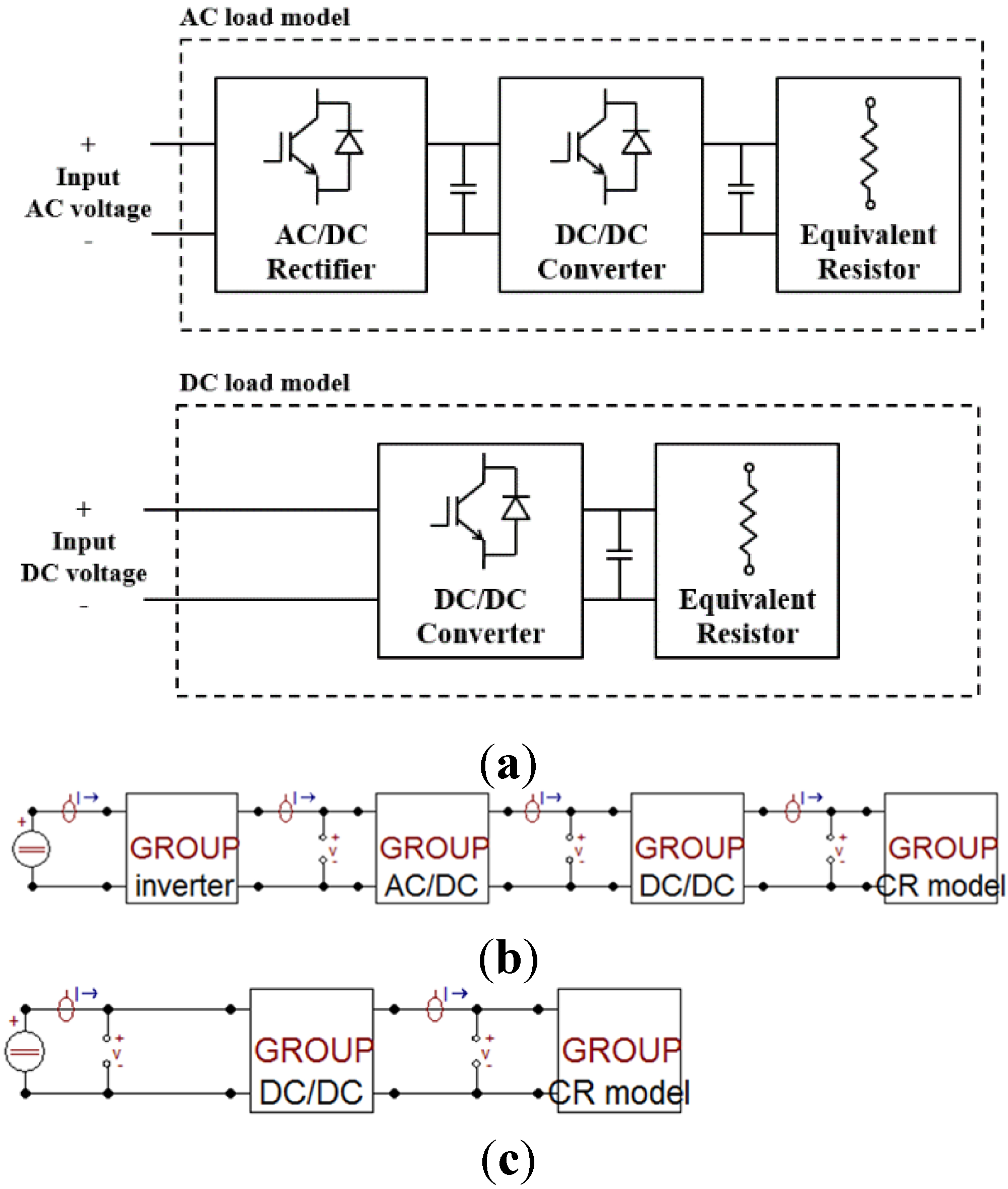
2.3. Load Modeling

In this part, the AC load and DC load with the power electronic converter are modeled [21,22]. This paper models the AC load using a rectifier, DC/DC converter, and equivalent resistor. The rectifier and DC/DC converter model used in load modeling are already presented in Section 2.1. In the case of DC loads, the rectifier is removed because the DC loads are directly supplied from DC source. Thus, a DC/DC converter is only connected in front of the equivalent resistor.

Based on the Figure 12a, the AC load and DC load modeling are conducted using EMTP as shown in Figure 12b,c, respectively. Some parameters for the load modeling and simulation are presented in Table 3.

Figure 12. (a) Configuration of AC load and DC load model; (b) AC load modeling using EMTP; and (c) DC load modeling using EMTP.

Figure 12. (a) Configuration of AC load and DC load model; (b) AC load modeling using EMTP; and (c) DC load modeling using EMTP.

Table 3. Simulation parameters.

Parameter		Value
DC Input Voltage		380 VDC
DC/AC Inverter	Output voltage	220 VAC,RMS, 60 Hz
	Amplitude modulation index (ma)	0.84
	Frequency modulation index (mf)	200
Switching Frequency		12 kHz
Efficiency of DC/DC Converter		95%
Voltage of Equivalent Resistance		12 VDC

Table 3. Simulation parameters.

Parameter		Value
DC Input Voltage		380 VDC
DC/AC Inverter	Output voltage	220 VAC,RMS, 60 Hz
	Amplitude modulation index (ma)	0.84
	Frequency modulation index (mf)	200
Switching Frequency		12 kHz
Efficiency of DC/DC Converter		95%
Voltage of Equivalent Resistance		12 VDC

In Table 4, the diode rectifier and the buck converter have approximately 75% and 91% efficiency, respectively. The total efficiency, which is calculated by multiplying both efficiencies together, is 68.67%. For the case of a DC load, the efficiency must be calculated only for the buck converter. Thus, the efficiency of the buck converter is the total efficiency, 90.44%. In conclusion, the DC load has higher efficiency in an LVDC distribution system than an AC load because of the reduction of the power conversion stage. The results show that, if the system requires high efficiency by adopting an LVDC distribution system, the existing AC load should be replaced with a DC load. That is, the efficiency of an LVDC distribution system can be improved by applying a DC load.

Table 4. Simulation results for an electronic load model at 14.4 W.

Load	Component	Factor	Value
AC Load	Diode Rectifier	Input Voltage	220 V
		Input Current	0.0953 A
		Input Power	20.97 W
		Efficiency	75.08%
	DC/DC Buck converter	Input Voltage	178.91 V
		Input Current	0.088 A
		Input Power	15.744 W
		Efficiency	91.46%
	Total efficiency		68.67%
DC Load	DC/DC Buck converter	Input Voltage	380 V
		Input Current	0.045 A
		Input Power	15.465 W
		Efficiency	90.44%

Table 4. Simulation results for an electronic load model at 14.4 W.

Load	Component	Factor	Value
AC Load	Diode Rectifier	Input Voltage	220 V
		Input Current	0.0953 A
		Input Power	20.97 W
		Efficiency	75.08%
	DC/DC Buck converter	Input Voltage	178.91 V
		Input Current	0.088 A
		Input Power	15.744 W
		Efficiency	91.46%
	Total efficiency		68.67%
DC Load	DC/DC Buck converter	Input Voltage	380 V
		Input Current	0.045 A
		Input Power	15.465 W
		Efficiency	90.44%

2.4. PV Generation System and ESS System Modeling

2.4.1. PV Generation System

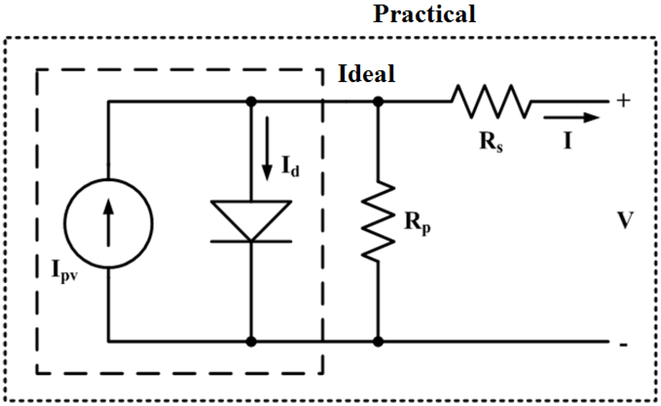
In order to model a PV system, we need to consider the characteristics of a PV cell. Generally, the PV array consists of the various PV cell. Figure 13 shows the equivalent circuit of PV cell, and we consider the I-V characteristic of a practical PV array, which includes series and parallel resistance [23]. The I-V characteristic of a practical PV array is expresses as Equation (1).

Figure 13. Equivalent circuit of PV cell.

Figure 13. Equivalent circuit of PV cell.

$$I=I_{pv}-I_0\left[\exp \left(\frac{V+R_{s}I}{V_{t}a}\right)-1\right]-\frac{V+R_{s}I}{R_p}$$

(1)

where I₀: Saturation current; V_t: Thermal voltage.

For determining the resistance connected to PV cell, Equations (2) and (3) can be used. Equation (2) is based on the fact that the series and parallel resistance value which warranties that maximum power of PV array model and maximum power of experimental data sheet are same is just one [24]. Thus, we firstly find the series and parallel resistance values that satisfy Equation (2), and then the calculation of I-V curve for series and parallel resistance must be conducted.

$$P_{\max ,m}=V_{mp}\left\{I_{pv}-I_{0}D-\frac{V_{mp}+R_s{I}_{mp}}{R_p}\right\}=P_{\max ,e}$$

(2)

$$D=\exp \left(\frac{q}{kT}\frac{V_{mp}+R_s{I}_{mp}}{a{N}_s}\right)-1$$

(3)

where P_max,m: Maximum power of PV array; P_max,e: Maximum power of experimental data sheet.

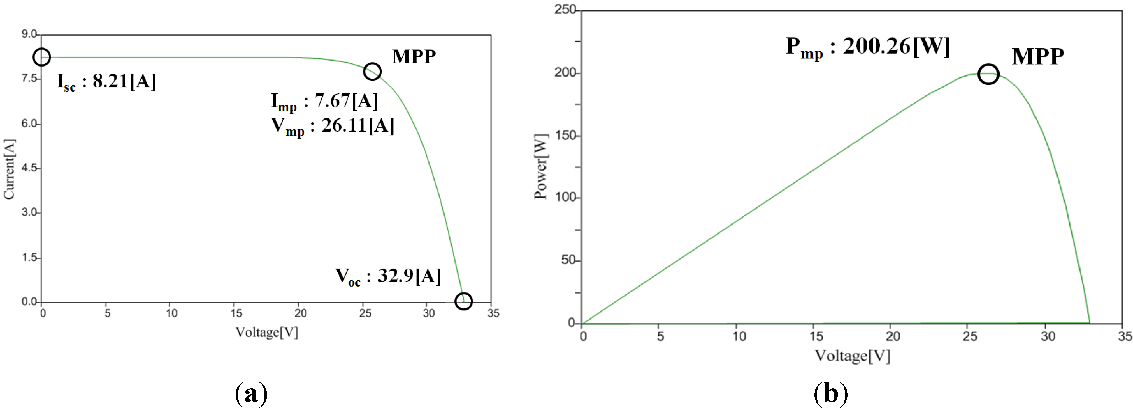
Based on the above content, we use EMTP to model PV arrays by applying the I-V characteristic of a PV cell. The output current or voltage of PV arrays considering parameters such as irradiation and temperature can be numerically and iteratively calculated, and algorithm for Maximum Power Point Tracking (MPPT) is implemented using EMTP/MODELS [24]. Figure 14 shows the calculated I-V and P-V characteristic curves of the PV array. From the Figure 14 and Table 5, we can find that the result of modeled PV array system is very similar to the experimental data sheet.

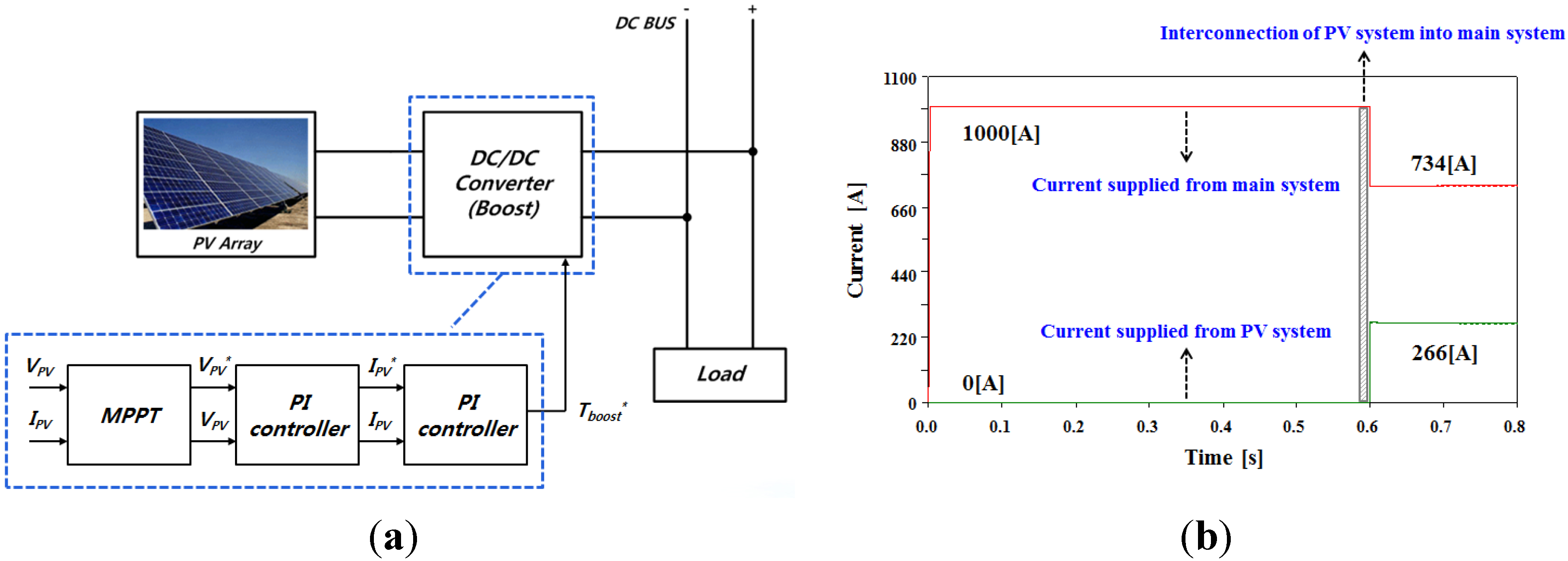
Figure 15a shows the concept of interconnection between a PV generation system and an LVDC distribution system. In Figure 15a, the duty rate of a DC/DC converter is determined by the MPPT algorithm, which is implemented using EMTP/MODELS. Furthermore, Figure 15b shows the current flow measured on the load side when the PV generation system is interconnected with the main DC system at certain times. As shown in the presented simulation result, a PV generation system normally supplies the current to a main system by distributing the current at the interconnection time. Thus, we can conclude that the modeled PV system is operated accurately as designed. Also, we might analyze the various effects when the PV generation system is connected to the LVDC system by using the PV generation system modeled in this part.

Figure 14. (a) I-V characteristic curve of the PV array; (b) P-V characteristic curve of the PV array.

Figure 14. (a) I-V characteristic curve of the PV array; (b) P-V characteristic curve of the PV array.

Table 5. Comparison of output of experimental data sheet and modeled PV array.

Output	ISC (A)	VOC (V)	Imp (A)	Vmp (V)	Pmp (W)
Data sheet	8.21	32.9	7.61	26.30	200.143
Model output	8.21	32.9	7.67	26.11	200.260
Error [%]	0	0	0.78	0.72	0.06

Table 5. Comparison of output of experimental data sheet and modeled PV array.

Output	ISC (A)	VOC (V)	Imp (A)	Vmp (V)	Pmp (W)
Data sheet	8.21	32.9	7.61	26.30	200.143
Model output	8.21	32.9	7.67	26.11	200.260
Error [%]	0	0	0.78	0.72	0.06

Figure 15. (a) Interconnection between a PV system and an LVDC distribution system; and (b) distribution of current by interconnecting a PV system into a main system.

Figure 15. (a) Interconnection between a PV system and an LVDC distribution system; and (b) distribution of current by interconnecting a PV system into a main system.

2.4.2. ESS System

Generally, the ESS is composed of a battery and a bi-directional DC/DC converter. According to the [25], it is recommended to use Li-ion battery when the ESS is utilized with the purpose of improving power quality and power system reliability. Thus, this paper models the Li-ion battery and the some parameters about ESS are presented in Table 6. In the case of bi-directional DC/DC converter, the model which is described in Section 2.1 is considered.

Table 6. Modeled ESS parameters.

ESS Energy (kWh)	ESS Power (kW)	Input and Output Voltage (V)	Input and Output Current (A)
100	20	500	40
200	40	500	80
250	50	500	100
500	100	500	200
1000	200	500	400

Table 6. Modeled ESS parameters.

ESS Energy (kWh)	ESS Power (kW)	Input and Output Voltage (V)	Input and Output Current (A)
100	20	500	40
200	40	500	80
250	50	500	100
500	100	500	200
1000	200	500	400

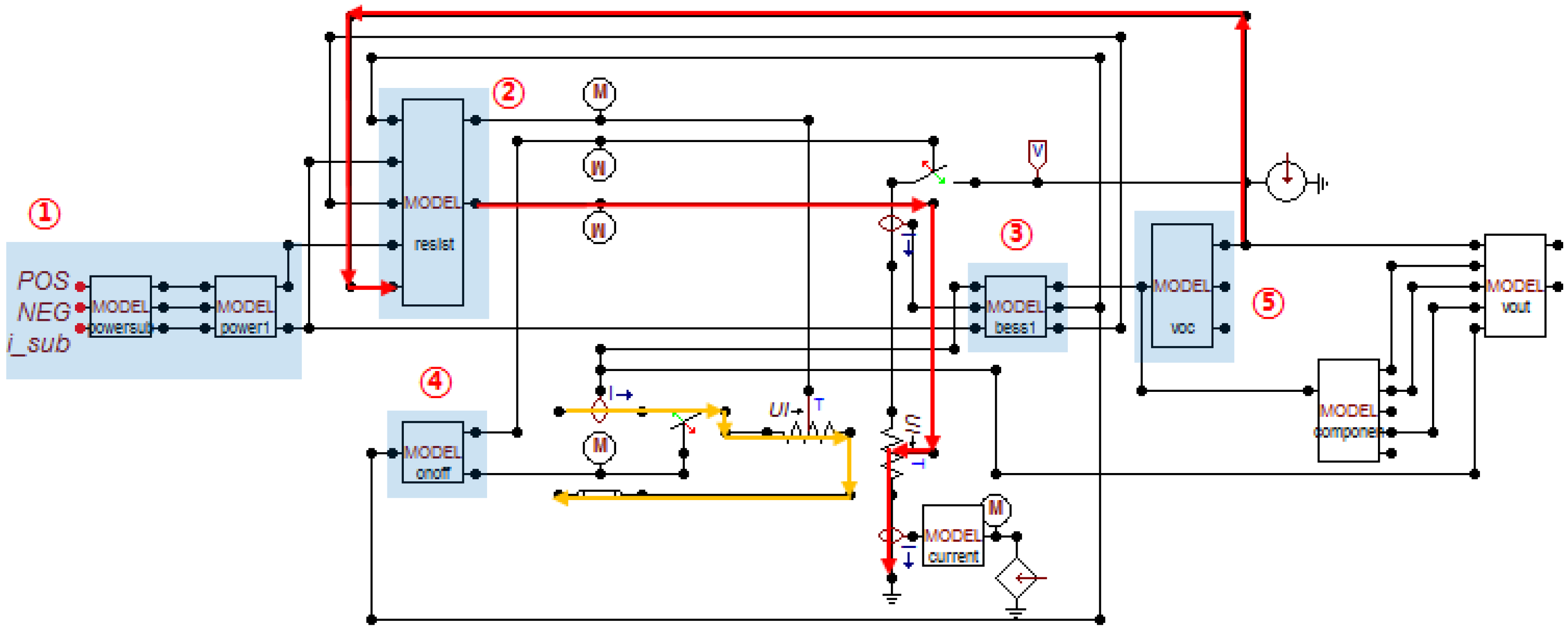
The ESS model is composed of a Li-ion battery and a bi-directional DC/DC converter. The ESS system modeled in this study using EMTP is presented in Figure 16. In Figure 16, some parameters such as the State of Charge (SoC), battery open circuit voltage, and internal resistance are mathematically expressed in EMTP/MODELS [26]. Each part of the ESS model is summarized as follows:

- ① :

Measurement of voltage and current/ Calculation of demand power

- ② :

Control of ESS input and output

- ③ :

Control of ESS operation algorithm

- ④ :

Control of ESS connection or ESS disconnection to main DC system

- ⑤ :

Calculation of Li-ion battery output voltage

Figure 16. Modeling of an ESS system using EMTP.

Figure 16. Modeling of an ESS system using EMTP.

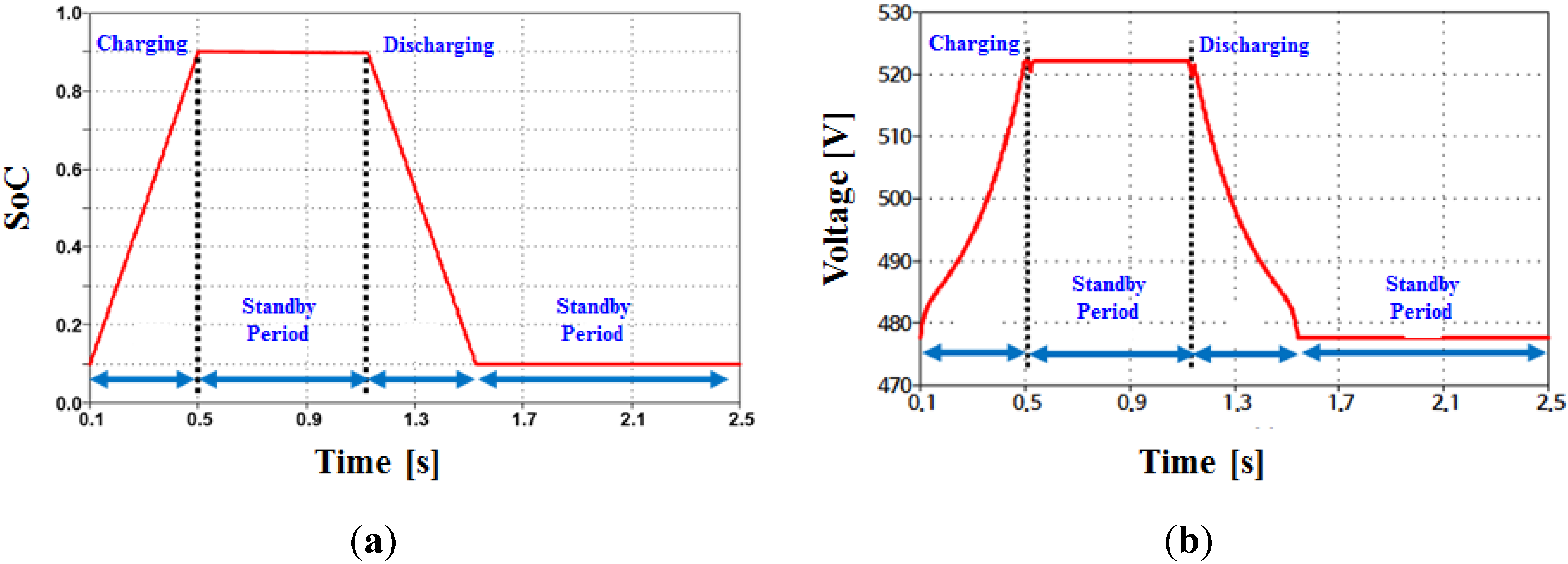
In Figure 16, the path denoted by a yellow line indicates the charging path of the ESS battery. The path marked with a red line shows the discharging path of the ESS battery. Part ②, which manages the control of the ESS input and output, receives the real-time system load as an input and then controls the output of the ESS using EMTP/MODELS. Figure 17 shows the SoC curve and the output voltage of the ESS. The charging and discharging modes of ESS are properly controlled according to the SoC, so that we can conclude that the modeled ESS system has good performance and it can be operated accurately as designed.

Figure 17. (a) SoC curve of ESS; (b) Output voltage of ESS.

Figure 17. (a) SoC curve of ESS; (b) Output voltage of ESS.

3. Analysis of Characteristics in Steady-State in an LVDC Distribution System

In this section, an analysis of the steady-state characteristics of an LVDC distribution system is presented. The test system for the simulation is composed of various components, which are modeled in Section 2. To study the steady-state characteristics, two case studies, which include load unbalance and interconnection of the PV generation system in an LVDC distribution system, are considered.

3.1. Analysis of Voltage and Load Unbalance in an LVDC Distribution System

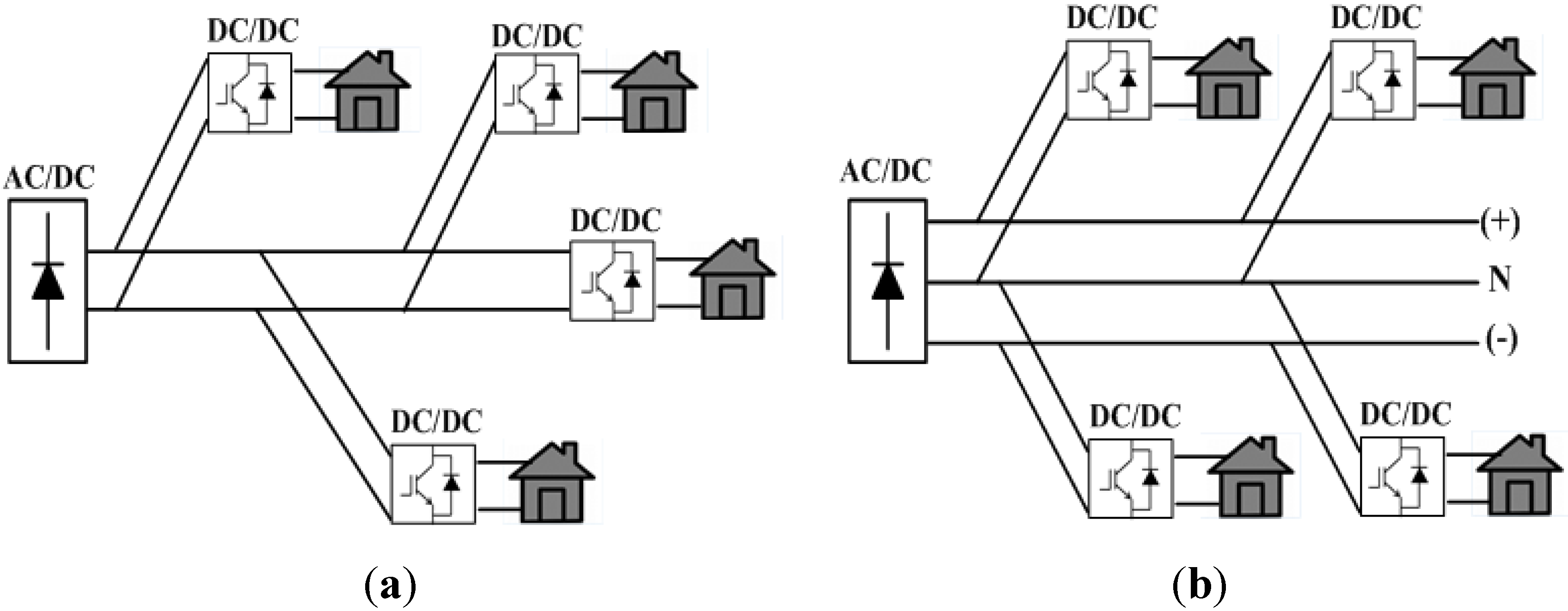
According to the number of poles in an LVDC distribution system, a system is either unipolar or bipolar, as shown in Figure 18 [6]. Three-voltage levels, which are positive-to-ground, negative-to-ground, and pole-to-pole voltage, can be used in a bipolar system with three wires. Thus, on the load side, the DC/DC converter selects the source voltage from three-voltage levels. In addition, a short circuit occurring on one load side does not affect the other loads, so a bipolar system can achieve a high-quality power supply. However, a bipolar system has problems such as the unbalance phenomenon: Unbalanced current flows into the neutral line, which causes power loss on the neutral line.

Figure 18. (a) Unipolar system; and (b) bipolar system.

Figure 18. (a) Unipolar system; and (b) bipolar system.

When the capacities of the load in two poles are different from each other, the system has an unbalanced load condition. Practically, because the use of electricity is constantly changing, it is impossible for a distribution system to maintain load balance. Unbalanced loads cause voltage unbalance in a distribution system. The customer load, which is mostly a single-pole load, can be changed continuously and, thus, incurs unintended voltage unbalance. Therefore, most distribution systems contain a certain level of voltage unbalance according to the system conditions. To express the severity of the load unbalance and voltage unbalance, load and voltage unbalance factors are generally used. Both factors are calculated by dividing the difference between the quantities at two poles by an average value. 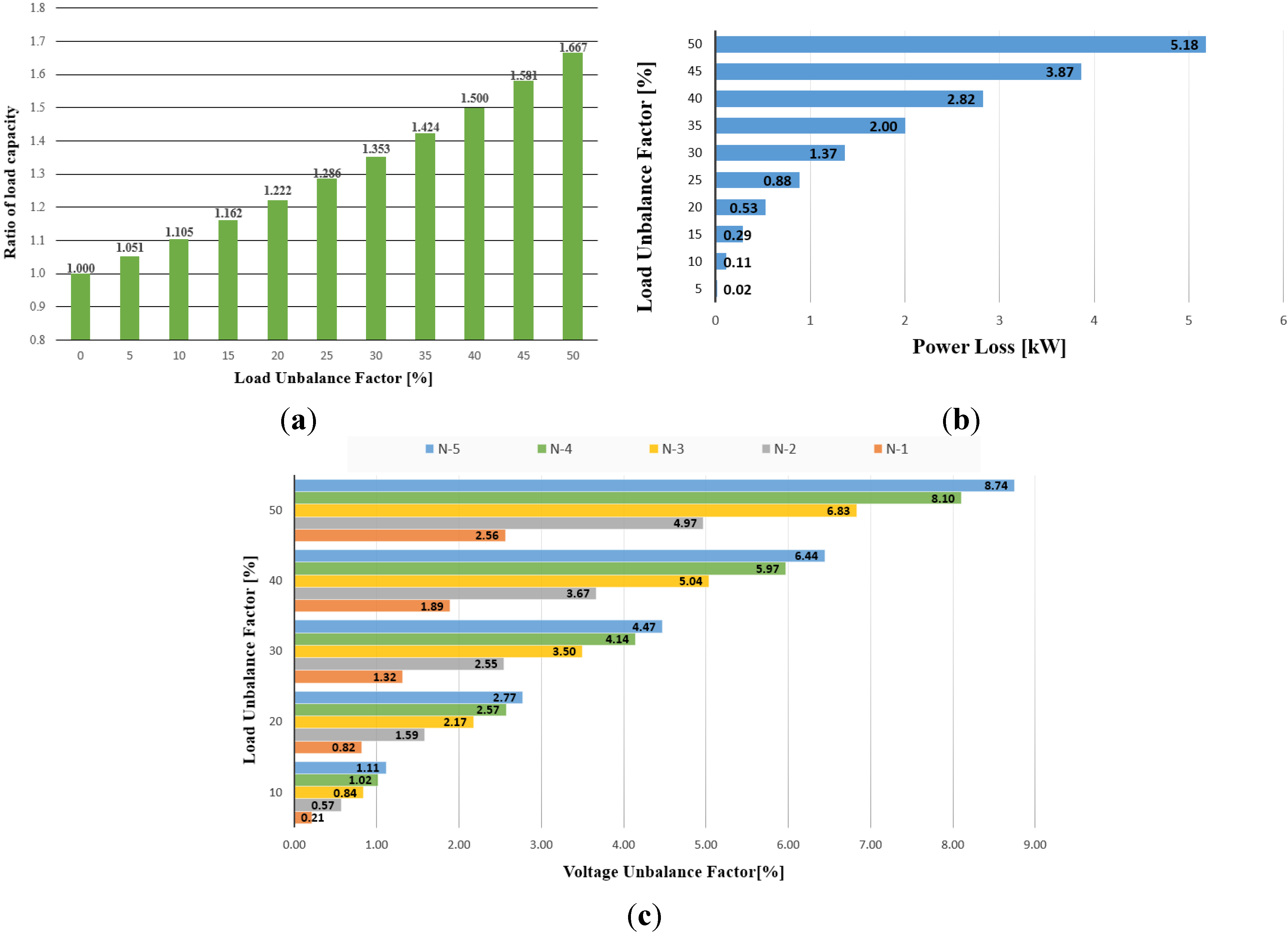Figure 19a shows the trend of the load unbalance factor according to the ratio of the load capacity, which is the ratio of the load capacity at a pole when the other load capacity is assumed to be one. The large difference between the two load capacities causes the high unbalanced load state. In Korean distribution systems, the load unbalanced factor is limited to 40%. For a simple bipolar distribution system with 500 kW load, Figure 19b presents the power loss on a neutral line caused by an unbalanced current according to the load unbalance factor. The power loss is influenced by the square of the unbalanced current and the line resistance. Thus, the LVDC distribution system with an excessive load unbalance factor has a significant amount of power loss. Lastly, Figure 19c shows the voltage unbalance factor according to the load unbalance factor. As expected, the high load unbalance begets a severe voltage unbalance. In addition, the load farthest from the power source, N-5, has the highest voltage unbalance factor. Here, load N-1 is closest to the power source.

Figure 19. (a) Ratio of load capacity according to load unbalance factor; (b) power loss on the neutral line according to load unbalance factor; and (c) voltage unbalance factor according to load unbalance factor.

Figure 19. (a) Ratio of load capacity according to load unbalance factor; (b) power loss on the neutral line according to load unbalance factor; and (c) voltage unbalance factor according to load unbalance factor.

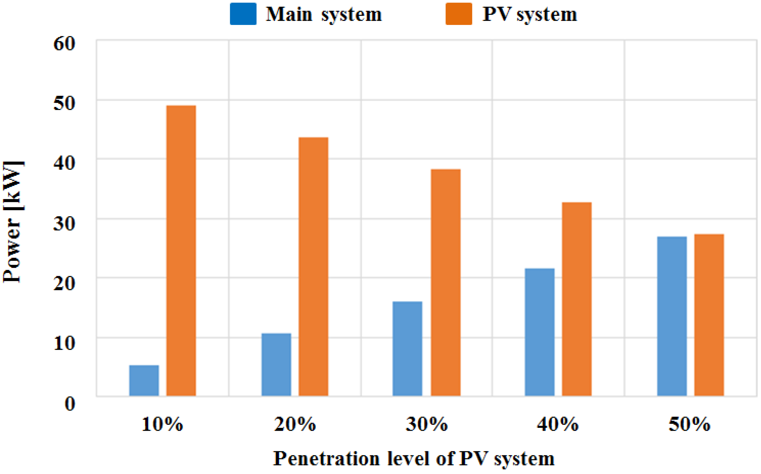
3.2. Analysis of Reverse Power Flow by Interconnection of a PV System with an LVDC Distribution System

In a power system, the distributed energy resource, including a PV system, plays a major role in the supply of power to the main system. However, there is a critical problem for applying distributed generation into the main power system. When the volume of the distributed generation is increased, the reverse power flow from the distributed generation can cause problems, such as a voltage rise at the distribution line [27]. Therefore, analysis of the reverse power flow due to the interconnection of the distributed energy resource with an LVDC distribution system is very important.

Generally, the occurrence of reverse power flow is mainly affected by both the capacity and location of distributed generation. This section deals with the analysis of reverse power flow caused by the interconnection of a PV system in an LVDC distribution system. In this case study, the output power of a PV system is changed according to the penetration level of the PV system, which is connected to the main system. If the penetration level of the PV system increases, the output power of the PV system also increases. On the other hand, the power that is supplied from the main system to the load side can be reduced though the interconnection of the PV system. Figure 20 shows the power distribution between the main system and the PV system according to the penetration level of the PV system.

Figure 20. Power distribution between the main system and PV system according to the penetration level of the PV system.

Figure 20. Power distribution between the main system and PV system according to the penetration level of the PV system.

The current flow according to penetration level of a PV system considering the location of the PV system is presented in Table 7 and Table 8. Table 7 shows the simulation result for Case 1, in which the PV system is installed in the nearest location to the power source. Table 8 indicates the current flow according to penetration level of the PV system for Case 2, where the PV system is installed farthest from the power source.

In Table 7 and Table 8, the current flow is measured at various locations in the LVDC system. Generally, as the penetration level of the PV system increases, more current produced by the PV system can be supplied to the main LVDC system. For each measured current, I_PV means the supplied current from the PV system to the main LVDC system. I_A is the current measured at the nearest location to the power source. Additionally, I_E is measured at the end of the load side. That is, the measuring point for I_E is at the furthermost end of the power source. If the PV system is installed at the location closest to the power source, as in Case 1, the current flows are considerably stable in most parts of the power system. In Case 1, there is reverse power flow at measuring point I_A, which is the nearest location to the power source when the penetration level of the PV system is only 50%. On the other hand, if the PV system is installed at the furthermost end of the power source, such as in Case 2, there are many reverse power flows at various measuring points regardless of the penetration level of the PV system. That is, the current flows are significantly unstable in many locations, and we expect that this phenomenon will affect the stability of the power system in terms of the system voltage.

Table 7. Current flow according to the penetration level of PV system—Case 1.

Penetration Level	PV System	Main System
	IPV (A)	IA (A)	IB (A)	IC (A)	ID (A)	IE (A)
10%	5.3469	13.252	13.938	8.7412	5.5306	2.7067
20%	10.718	9.097	13.807	8.1953	5.362	3.0286
30%	16.147	5.2707	13.845	8.4679	5.5082	2.872
40%	21.545	2.0244	13.932	8.3401	5.7503	2.7137
50%	27	−1.8334	13.676	7.873	5.3046	3.01

Table 7. Current flow according to the penetration level of PV system—Case 1.

Penetration Level	PV System	Main System
	IPV (A)	IA (A)	IB (A)	IC (A)	ID (A)	IE (A)
10%	5.3469	13.252	13.938	8.7412	5.5306	2.7067
20%	10.718	9.097	13.807	8.1953	5.362	3.0286
30%	16.147	5.2707	13.845	8.4679	5.5082	2.872
40%	21.545	2.0244	13.932	8.3401	5.7503	2.7137
50%	27	−1.8334	13.676	7.873	5.3046	3.01

Table 8. Current flow according to the penetration level of PV system—Case 2.

Penetration Level	PV System	Main System
	IPV (A)	IA (A)	IB (A)	IC (A)	ID (A)	IE (A)
10%	5.3469	13.122	10.455	4.8462	1.6026	−0.75044
20%	10.718	9.1231	6.4522	0.8022	−1.7459	−4.7446
30%	16.147	5.4109	2.6408	−3.0168	−5.3671	−7.9439
40%	21.545	1.934	−1.092	−6.0445	−9.824	−11.584
50%	27	−1.9489	−5.253	−10.492	−12.997	−16.12

Table 8. Current flow according to the penetration level of PV system—Case 2.

Penetration Level	PV System	Main System
	IPV (A)	IA (A)	IB (A)	IC (A)	ID (A)	IE (A)
10%	5.3469	13.122	10.455	4.8462	1.6026	−0.75044
20%	10.718	9.1231	6.4522	0.8022	−1.7459	−4.7446
30%	16.147	5.4109	2.6408	−3.0168	−5.3671	−7.9439
40%	21.545	1.934	−1.092	−6.0445	−9.824	−11.584
50%	27	−1.9489	−5.253	−10.492	−12.997	−16.12

4. Analysis of Characteristics in the Transient State in an LVDC Distribution System

In this section, an analysis of the characteristics in the transient state of an LVDC distribution system is discussed. For studying the characteristics in the transient state, two case studies, which include a line fault and a series arc fault in an LVDC distribution system, are considered.

4.1. Analysis of a Series Arc Fault in an LVDC Distribution System

Generally, a series arc fault occurs when there is a discontinuity in the electrical path due to loosened connectors or terminals, but the current continues to flow [28,29]. From the electrical point of view, a series arc is considered as an additional resistance, which is a series arc resistance, and it increases the equivalent circuit resistance, which means a decrease in the current flowing through the circuit. 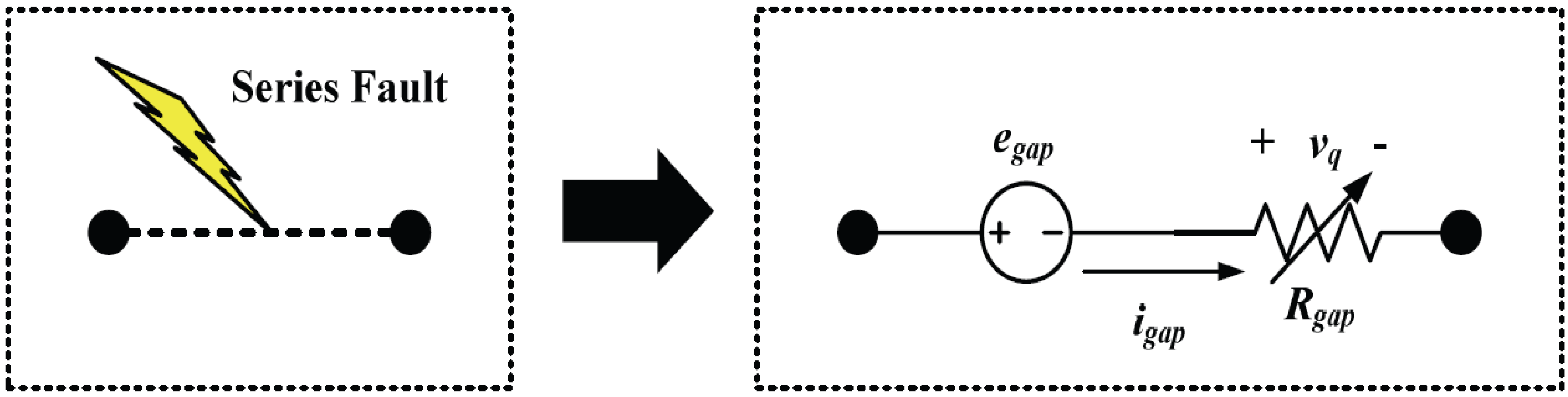Figure 21 shows the equivalent series arc model based on the mathematical approximation model. As indicated in Figure 21, the series arc can be represented as two components: an electromotive force pulse, e_gap, and a nonlinear resistor, R_gap. Mathematical expressions for each component in Figure 21 are presented in [30].

Figure 21. Equivalent model of a series arc [30]. Notes: e_gap: electromotive force pulse; i_gap: current through gap; R_gap: series arc resistance.

Figure 21. Equivalent model of a series arc [30]. Notes: e_gap: electromotive force pulse; i_gap: current through gap; R_gap: series arc resistance.

Based on the mathematical model, we simulate the DC series arc fault. The model is implemented using EMTP/MODELS [31], and the series arc fault is assumed to occur at the load end where a very low voltage is applied, because this kind of fault is uncommon at higher voltage levels. We divide the simulation cases according to the various fault types and event sequences as shown in Table 9.

Table 9. Case study for series arc fault in an LVDC distribution system.

Case No.	Fault Type	First Event	Second Event
Case 3	Fixed gap distance fault	Fault	-
Case 4	Constant gap speed fault	Fault	-
Case 5	Fixed gap distance fault	Load injection	Fault
Case 6	Constant gap speed fault	Load injection	Fault

Table 9. Case study for series arc fault in an LVDC distribution system.

Case No.	Fault Type	First Event	Second Event
Case 3	Fixed gap distance fault	Fault	-
Case 4	Constant gap speed fault	Fault	-
Case 5	Fixed gap distance fault	Load injection	Fault
Case 6	Constant gap speed fault	Load injection	Fault

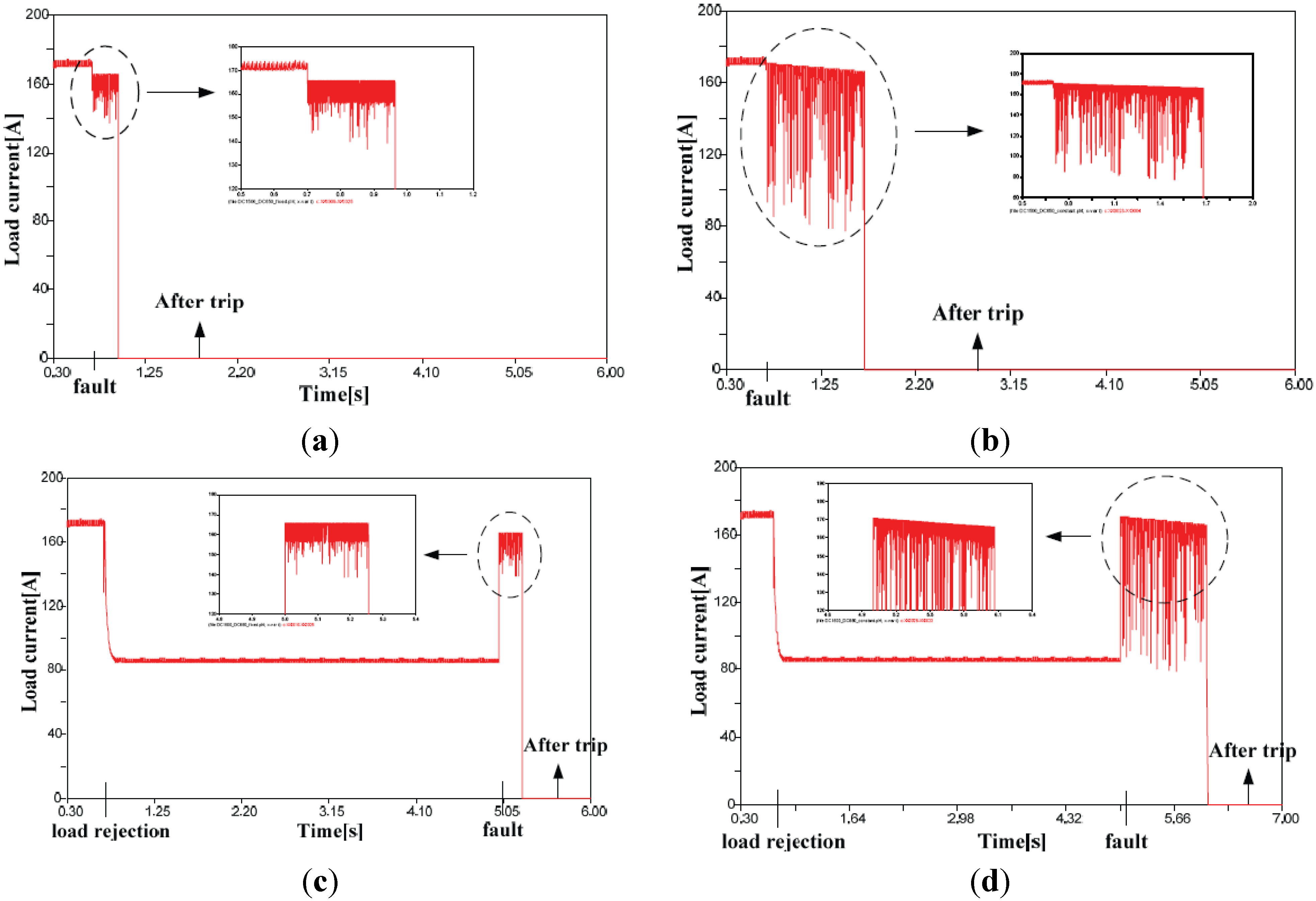
Figure 22 shows the load current for all case studies. Each result shows a different characteristic according to the fault condition [31]. The series arc has a random characteristic, which is represented as a very “spiky” profile in the current waveform. The “spiky” profile represents a repetitive extinction and re-ignition of the arc. For all of the simulation cases, the fluctuant “spiky” profile was produced at the fault inception time regardless of the fault type or the occurrence of successive events. These faults prevent circuit breakers from responding in a timely fashion to such a low fault current due to a series arc fault. Therefore, it might be necessary to detect the series fault in order to protect the circuits.

4.2. Analysis of a Line Fault in an LVDC Distribution System

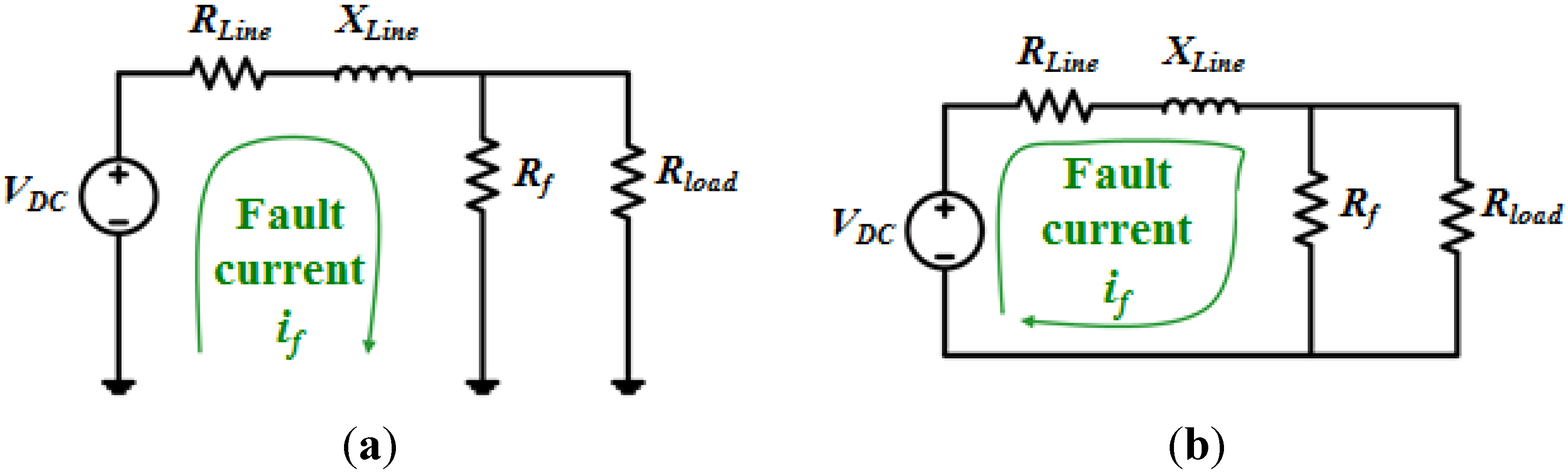
Generally, there are two types of line faults in an LVDC distribution system: (1) Pole to Ground (PTG) faults and (2) Pole to Pole (PTP) faults. A PTG fault occurs when either the positive or negative pole is short-circuited to the ground. A PTP fault occurs when a path between the positive and negative poles is created, short-circuiting them together [32]. If any type of fault happens, the fault path is formed according to the type of fault, as shown in Figure 23. In a faulted circuit, the fault current i_f can be defined as in Equation (4).

Figure 22. (a) Simulation result for Case 3; (b) Simulation result for Case 4; (c) Simulation result for Case 5; (d) Simulation result for Case 6 [31].

Figure 22. (a) Simulation result for Case 3; (b) Simulation result for Case 4; (c) Simulation result for Case 5; (d) Simulation result for Case 6 [31].

Figure 23. (a) Path of the fault current in a PTG fault; (b) Path of the fault current in a PTP fault.

Figure 23. (a) Path of the fault current in a PTG fault; (b) Path of the fault current in a PTP fault.

$$i_f=\frac{V_{DC}}{R_{eq}}(1-e^{-\frac{R_{eq}}{L}t})$$

(4)

where V_DC: DC voltage; R_eq: Equivalent resistance in voltage source; L: Line impedance.

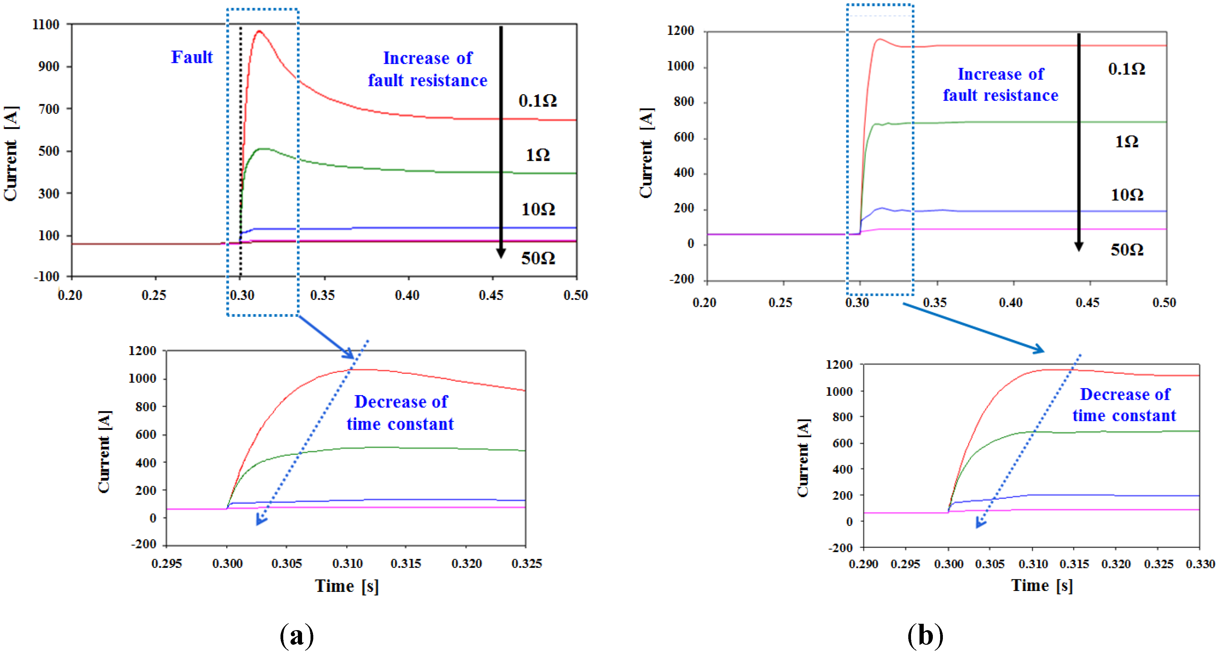
From Equation (4), we can see that the magnitude of the fault current is determined according to the variation of the equivalent resistance in the faulted circuit. The time constant (R_eq/L), which refers to the decay time of the transient element, is also affected by the equivalent resistance. In Figure 23, the pre-fault equivalent resistance can be expressed as the sum of the line resistance and the load resistance. However, the post-fault equivalent resistance is changed as shown in Equation (5) after a fault due to the parallel connection of the fault resistance. Equation (5) can be changed to Equation (6), and the equivalent resistance is proportional to the fault resistance (R_f) in Equation (6). Therefore, the fault current and time constant decrease when a fault occurs.

$$R_{eq}=R_{Line}+R_{load}//R_f$$

(5)

$$R_{eq}=R_{Line}+R_{load}//R_f=R_{Line}+\frac{R_{load}\times R_f}{R_{load}+R_f}$$

(6)

Figure 24 a,b shows the fault current and time constant according to the fault resistance in the cases of PTG and PTP faults, respectively. The simulation results show that the magnitude of the fault current significantly decreases when the fault resistance increases. Additionally, it might be possible to apply the conventional relay scheme, which uses an over-current element for protecting the LVDC distribution system when the fault occurs with low resistance. However, there is a problem in applying the conventional relay scheme for a fault with high resistance because the variation of the fault current is extremely small and fast. Therefore, a new protective relaying system that uses another element instead of an over-current element must be developed in order to protect the LVDC distribution system in the case of a high-resistance fault.

Figure 24. (a) Fault current and time constant according to the fault resistance in a PTG fault; (b) fault current and time constant according to the fault resistance in a PTP fault.

Figure 24. (a) Fault current and time constant according to the fault resistance in a PTG fault; (b) fault current and time constant according to the fault resistance in a PTP fault.

5. Conclusions

In this paper, the modeling and analysis of an LVDC distribution system are conducted. For the modeling of an LVDC distribution system, the various essential components, such as power electronic devices, DERs, and ESSs that should be considered when implementing an LVDC distribution system, are modeled using EMTP. The modeled components are implemented using EMTP/MODELS, which is a symbolic language interpreter for EMTP. Based on the modeled LVDC distribution system, the steady-state simulation, such as the load unbalance and the connection of the PV generation system as a DER, is performed, and the analysis of the characteristics in those states is performed. Furthermore, the simulation and analysis of the transient state in the LVDC distribution system considering line faults and series arc faults are also presented. By applying the LVDC model presented in this paper, we can expect more realistic and effective analysis results for more various steady states and transient states as well as load unbalance, connection of PV, series arc faults, and line faults, which are also considered in this study.

References

- Brenna, M.; Lazaroiu, G.C.; Tironi, E. High Power Quality and DG Integrated Low Voltage DC Distribution System. In Proceedings of the IEEE Power Engineering Society General Meeting, Montreal, QC, Canada, 18–22 June 2006.
- Alessandro, A.; Morris, B.; Giuseppe, S.; Enrico, T.; Giovanni, U. LV DC Distribution Network with Distributed Energy Resources: Analysis of Possible Structures. In Proceedings of the International Conference on Electricity Distribution CIRED, Turin, Italy, 6–9 June 2005.
- Agustoni, A.; Borioli, E.; Brenna, M.; Simioli, G.; Tironi, E.; Ubezio, G. LVDC Distribution Network with Distributed Energy Resources: Analysis of Possible Structures. In Proceedings of the International Conference on Electricity Distribution CIRED, Turin, Italy, 6–9 June 2005.
- Byeon, G.; Yoon, H.L.T.; Jang, G.; Chae, W.; Kim, J. A research on the characteristics of fault current of DC distribution system and AC distribution system. In Proceedings of the IEEE International Conference on Power Electronics—ECCE Asia, Jeju, Korea, 30 May 2011–3 June 2011.
- Kaipia, T.; Salonen, P.; Lassila, J.; Partanen, J. Possibilities of the low voltage DC distribution systems. In Proceedings of the Nordic Distribution and Asset Management Conference (NORDAC 2006), Stockholm, Sweden, 21–22 August 2006.
- Salonen, P.; Kaipia, T.; Nuutinen, P.; Peltoniemi, P.; Partanen, J. An LVDC distribution system concept. In Proceedings of the Nordic Workshop on Power and Industrial Electronics, Espoo, Finland, 9–11 June 2008.
- Nilsson, D.; Sannino, A. Efficiency analysis of low and medium voltage DC distribution systems. In Proceedings of the IEEE Power Engineering Society General Meeting, Denver, CO, USA, 6–10 June 2004.
- Sannino, A.; Postiglione, G.; Bollen, M. Feasibility of a DC network for commercial facilities. IEEE Trans. Ind. Appl. 2003, 39, 1499–1507. [Google Scholar] [CrossRef]
- Salonen, P.; Kaipia, T.; Nuutinen, P.; Peltoniemi, P.; Partanen, J. Fault Analysis of LVDC Distribution System. In Proceedings of the International World Energy System Conference, Lasi, Romania, 30 June–2 July 2008.
- Brenna, M.; Tironi, E.; Ubezio, G. Proposal of a local DC distribution network with distributed energy resources. In Proceedings of the IEEE International Conference on Harmonics and Quality of Power, New York, NY, USA, 12–15 September 2004.
- Nilsson, D. DC Distribution Systems. Ph.D. Thesis, Chalmers University of Technology, Gotenborg, Sweden, 2005. [Google Scholar]
- Kazmierkowski, M.P.; Malesani, L. Current control techniques for three-phase voltage-source PWM converters: a survey. IEEE Trans. Ind. Electron. 1998, 45, 691–703. [Google Scholar] [CrossRef]
- Dixon, J.W.; Ooi, D.T. Indirect Current Control of a Unity Power Factor Sinusoidal Current Boost Type Three-phase Rectifier. IEEE Trans. Ind. Electron. 1998, 35, 508–515. [Google Scholar] [CrossRef]
- Noh, E.C.; Jung, G.B.; Choi, N.S. Power Conversion System, Power Electronics, 3rd ed.; Munundang: Seoul, Korea, 2011; pp. 311–413. [Google Scholar]
- Betten, J.; Kollman, R. Interleaving DC-DC Converters Boost Efficiency and Voltage; Texas Instruments: Attleboro, MA, USA, 2005. [Google Scholar]
- Jeong, H.J. Control of 3 Phase Interleaved Bidirectional DC/DC Converter for EV. Master’s Thesis, Sungkyunkwan University, Suwon, Korea, February 2011. [Google Scholar]
- Andrzej, M. Trzynadlowski, Introduction to Modern Power Electronics; WILEY: Hoboken, NJ, USA, 2010. [Google Scholar]
- Finnish Standards Association SFS 4879-0.6/1 kV power cables. XLPE-insulated Al-cables. Construction and testing; SESKO Standardization: Helsinki, Finland.
- Finnish Standards Association SFS 4880-0.6/1 kV power cables. PVC-insulated PVC-sheathed cables. Construction and testing; SESKO Standardization: Helsinki, Finland.
- Kim, E.S. Present Situation and Prospect of DC Distribution Technology. In Journal of the Electrical World/Monthly Magazine; Seoul, Korea, April 2010; pp. 61–65. [Google Scholar]
- Salomonsson, D; Sannino, A. Low-Voltage DC Distribution System for Commercial Power Systems with Sensitive Electronic Loads. IEEE Trans. Power Deliv. 2007, 22, 1620–1627. [Google Scholar]
- Seo, G.; Baek, J.; Choi, K.; Bae, H.; Cho, B. Modeling and analysis of DC distribution systems. In Proceedings of the IEEE 8th International Conference on Power Electronics and ECCE Asia (ICPE & ECCE), Jeju, Korea, 30 May 2011–3 June 2011.
- Rauschenbach, H.S. Solar Cell Array Design Handbook; Van Nostrand Reinhold: New York, NY, USA, 1980. [Google Scholar]
- Villalva, M.G.; Gazoli, J.R.; Filho, E.R. Comprehensive Approach to Modeling and Simulation of Photovoltaic Arrays. IEEE Trans. Power Electron. 2009, 24, 1198–1208. [Google Scholar] [CrossRef]
- Electric Power Research Institute (EPRI). Price Elasticity of Demand for Electricity: A Primer and Synthesis; Technical Report; EPRI: Palo Alto, CA, USA, January 2008. [Google Scholar]
- Kim, J.H.; Lee, S.J.; Kim, E.S.; Kim, S.K.; Kim, C.H.; Prikler, L. Modeling of Battery for EV using EMTP/ATPDraw. J. Electr. Eng. Technol. 2014, 9, 98–105. [Google Scholar] [CrossRef]
- Hatta, H.; Asari, M.; Kobayashi, H. Study of Energy Management for Decreasing Reverse Power Flow from Photovoltaic Power Systems. In Proceedings of the IEEE PES/IAS Conference on Sustainable Alternative Energy (SAE), Valencia, Spain, 28–30 September 2009.
- Potter, T.E.; Lavado, M. Arc Fault Circuit Interruption Requirements for Aircraft Applications; Texas Instruments: Attleboro, MA, USA, 2005. [Google Scholar]
- Schoepf, T.J.; Naidu, M.; Gopalakrishnan, S. Mitigation and analysis of arc faults in automotive DC networks. IEEE Trans. Compon. Packag. Technol. 2005, 28, 319–326. [Google Scholar] [CrossRef]
- Uriarte, F.M.; Gattozzi, A.L.; Herbst, J.D.; Estes, H.B.; Hotz, T.J.; Kwasinsky, A.; Hebner, R.E. DC Arc Model for Series Faults in Low Voltage Microgrids. IEEE Trans. Smart Grid 2012, 3, 2063–2070. [Google Scholar] [CrossRef]
- Oh, Y.S.; Han, J.; Gwon, G.H.; Kim, D.W.; Kim, C.H. Development of Fault Detector for Series Arc Fault in Low Voltage DC Distribution System using Wavelet Singular Value Decomposition and State Diagram. J. Electr. Eng. Technol. 2015, 10, 766–776. [Google Scholar] [CrossRef]
- Park, J.D.; Candelaria, J. Fault detection and isolation in low voltage DC-bus microgrid system. IEEE Trans. Power Deliv. 2013, 28, 779–787. [Google Scholar] [CrossRef]
© 2015 by the authors; licensee MDPI, Basel, Switzerland. This article is an open access article distributed under the terms and conditions of the Creative Commons Attribution license (http://creativecommons.org/licenses/by/4.0/).