
A Markov-Switching Vector Autoregressive Stochastic Wind Generator for Multiple Spatial and Temporal Scales

Abstract
:1. Introduction
2. Stochastic Wind Generator Model
2.1. Markov-Switching Vector Autoregressive Model
- The original and components for and do not follow a Gaussian distribution, so they are first each transformed to normality with a Gaussian copula as follows:
- (a)
- The empirical cumulative distribution function (ecdf) of each component of is obtained with:and similarly for , where is the indicator function that is unity, if the set condition holds, and is zero otherwise.
- (b)
- The transformed values of , denoted , are , and similarly for , where is the inverse of the standard normal cumulative distribution function.
- Then, we remove the seasonality and diurnal variability from the transformed and components of individually using a generalized additive model (GAM) [43] with:where is the month of the year, is the day of the year and is the hour of the day for observation t, and similarly for . The function is a penalized regression spline, which is the default in the R mgcv package [44]. Define detrended residuals as and , and the corresponding detrended vector is . The diurnal wind cycle can have a substantial impact on sizing and modeling integrated renewable systems, so it is important to model it properly [32,45,46], but note that the term is removed from Equation (2) when fitting a trend for the daily averages.
- Depending on the number of locations wherein it is desired to simulate the wind vector, we take one of two approaches to choosing the number of “regimes” in the Markov-switching model.
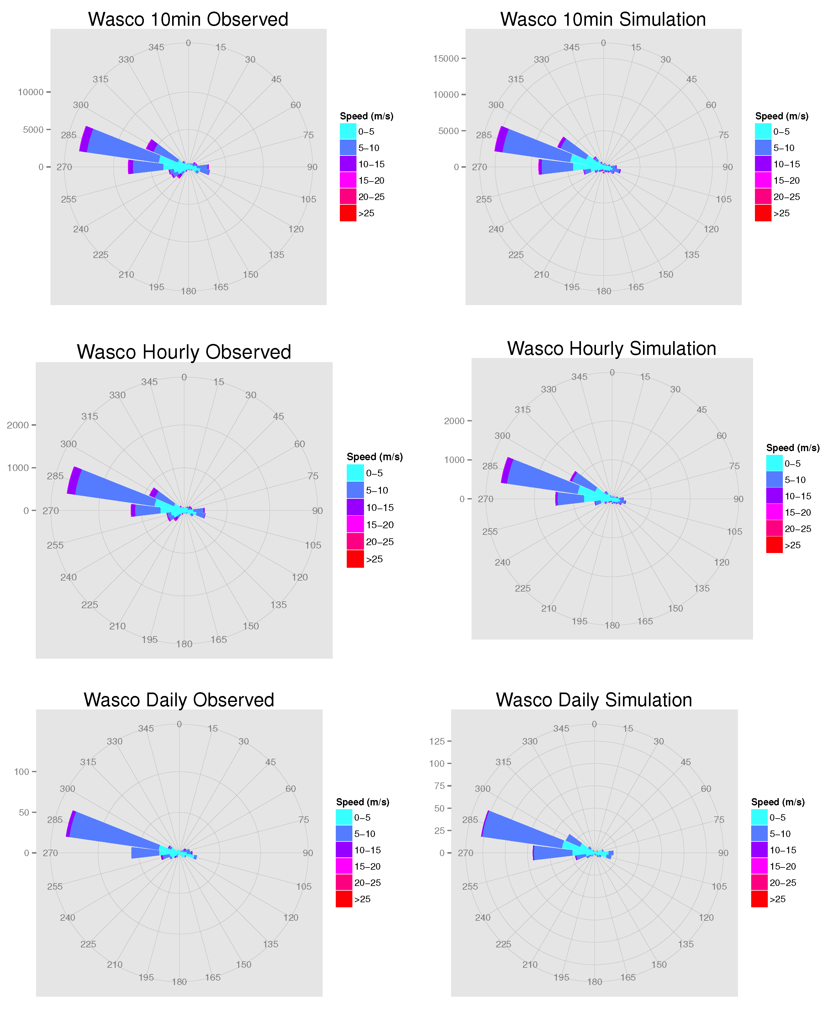
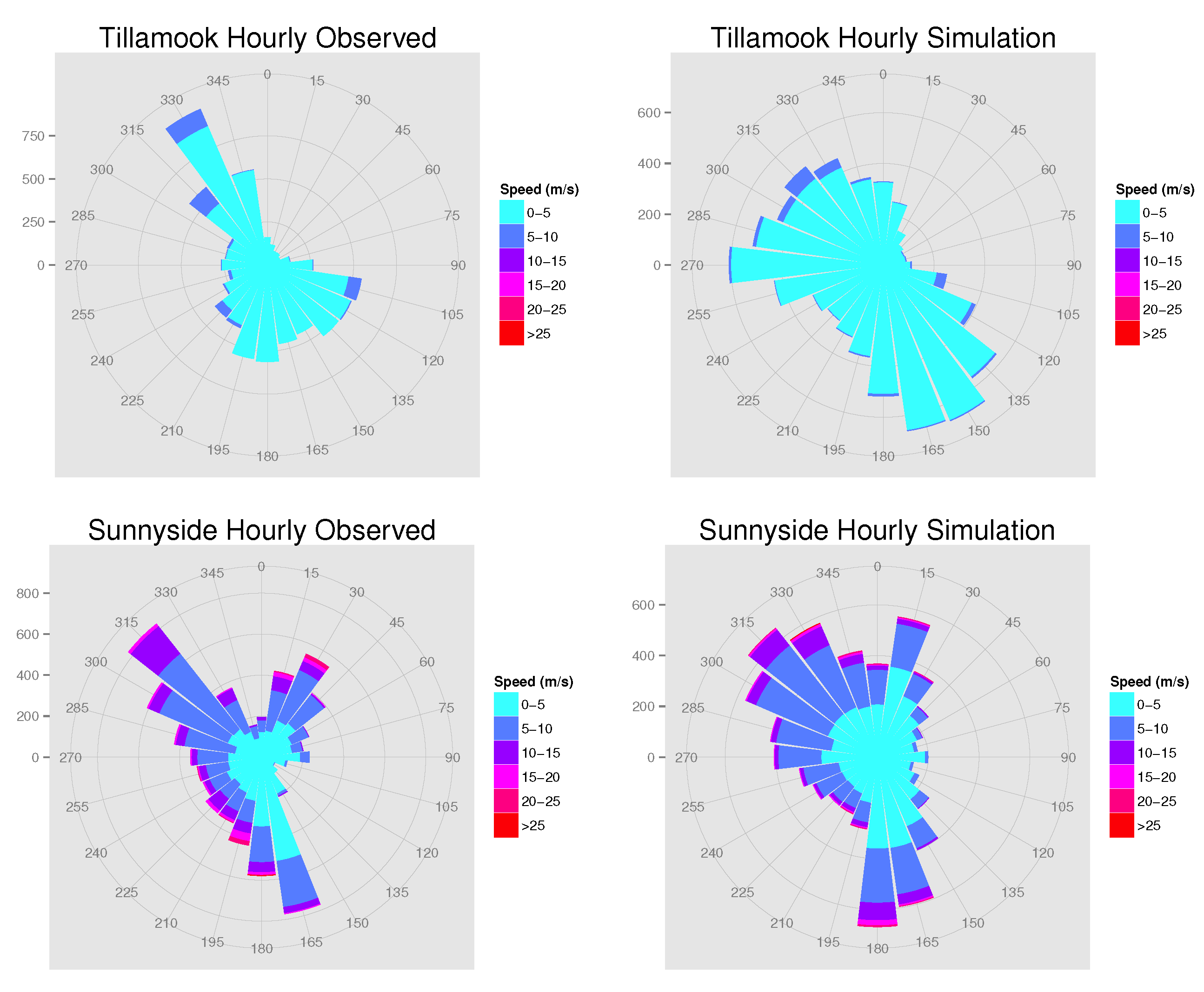
- : Plot the wind rose of the observed wind speed and direction. Let the number of modes in the joint distribution of speed and direction be the number of regimes.
- : Average the observed wind speed and wind directions across all p sites at each time t. Plot the wind rose of the averaged speed and directions, and let the number of regimes equal the number of modes in the joint distribution. Note that the circular mean of directions is taken whenever an average of directions is required [47].
- Given the number of regimes, K, we must classify the observations belonging to each one. We do this with an unconstrained Gaussian mixture model (GMM) clustering approach [48] applied to the observed transformed u and v components, and . Here, the components of the mixture model are assumed to be multivariate normal distributions with means , covariance matrices and mixing proportions for . The GMM is able to model ellipsoidal clusters of any size and orientation. We use the mclust package in R to perform the clustering [49], but we note here that clustering the 10-min data, which has 52,560 observations, fails, due to the size of the dataset. Thus, we cluster the hourly data and apply each hour’s cluster assignment to all 10-min observations within the corresponding hour. Secondly, when , we construct two sets of regimes based on the following sets of values:
- (a)
- the mean of the transformed u and v components across all p locations, defined as and for ; and
- (b)
- the transformed u and v components of all p locations,
- Use the subsets of observations identified in Step 4 to obtain least-squares estimates of the parameters in Equation (3), the Markov-switching autoregressive model (MSVAR) of order one:where the lag-one autoregressive matrix and innovation covariance matrix depend on the regime, . We let be a Markov chain on finite space, , that indicates the regime at time t. The regime-switching process is defined by a transition probability matrix , , where , and for all j.
- The transition probability matrix, , is estimated using the identified clusters and the observed proportion of instances in which the cluster assignments switch,The coefficient matrices, , are estimated using least-squares with the lm command in R based on the observations with regime . We note that the eigenvalues of must be positive in order for the VAR model to be stable; we did not encounter any difficulties in estimating these coefficients with the lm command, but any issues in estimation can be dealt with by using a constrained least squares estimation of . The variability matrix, , is estimated with the standard covariance estimator of the residuals of the model within each regime.
- Given the parameter estimates of , and from Step 6, simulate a new set of values, denoted , from Equation (3).
- Add back the estimated trend from Equation (2) to obtain:
- Transform the back into the original units by:and similarly for to obtain . Now, we have a simulated set of u and v components at p locations.
- As a final step, we convert the u and v components of into speed and direction, as these are usually more interpretable quantities upon which to perform validation.
3. Simulation Scenarios
3.1. Data Description

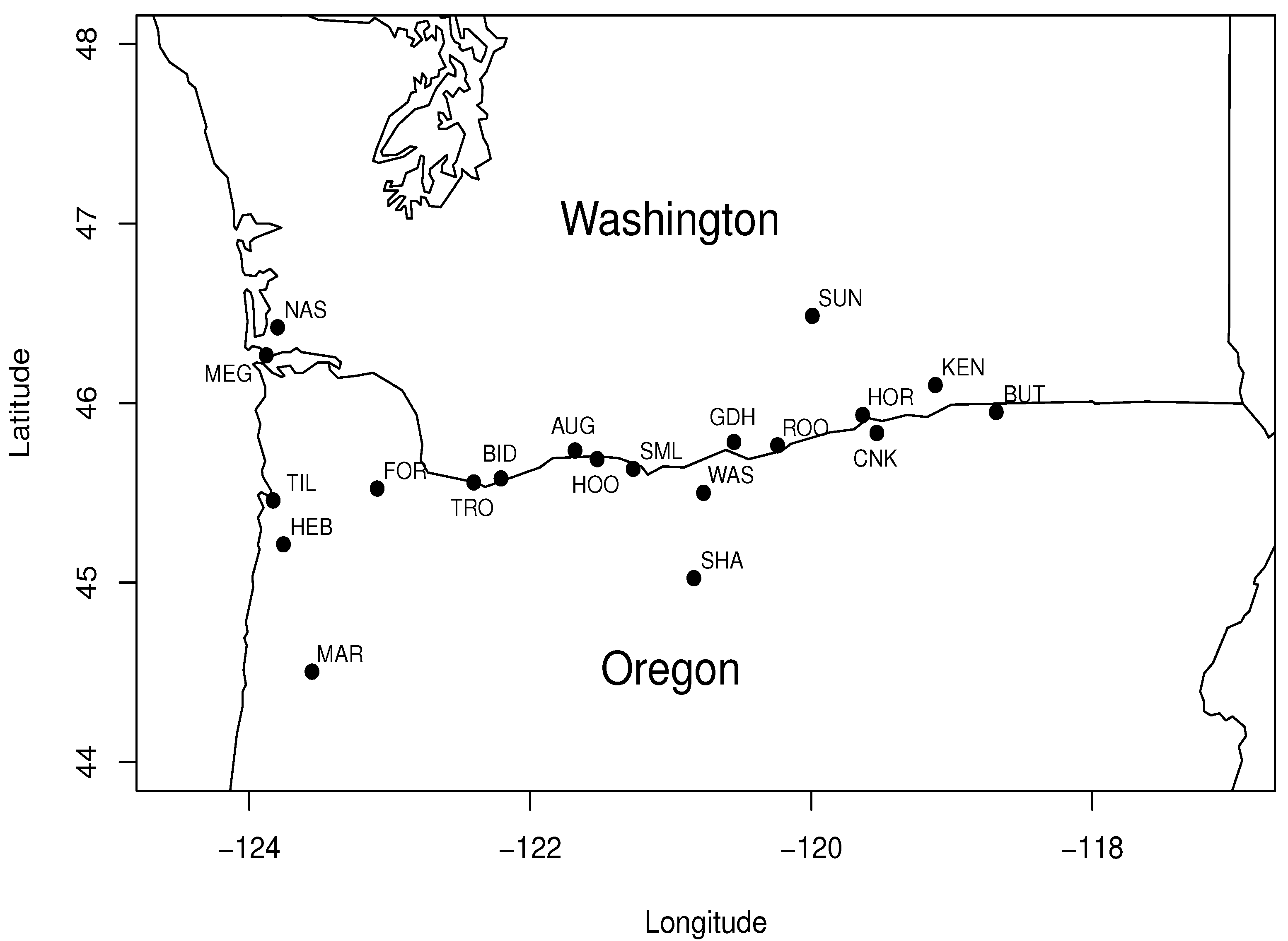
| Acronym | Name | 10-min | Hourly | Daily |
|---|---|---|---|---|
| AUG | Augspurger | 1,422 | 236 | 9 |
| BID | Biddle Butte | 0 | 0 | 0 |
| BUT | Butler Grade | 2,690 | 444 | 14 |
| CNK | Chinook | 2,687 | 444 | 14 |
| FOR | Forest Grove | 0 | 0 | 0 |
| GDH | Goodnoe Hills | 2,687 | 444 | 14 |
| HOO | Hood River | 0 | 0 | 0 |
| HOR | Horse Heaven | 0 | 0 | 0 |
| KEN | Kennewick | 0 | 0 | 0 |
| MAR | Mary’s Peak | 4,081 | 673 | 23 |
| MEG | Megler | 0 | 0 | 0 |
| HEB | Mt. Hebo | 2,148 | 351 | 12 |
| NAS | Naselle Ridge | 201 | 30 | 0 |
| ROO | Roosevelt | 281 | 46 | 1 |
| SML | Seven Mile Hill | 2,687 | 444 | 14 |
| SHA | Shaniko | 199 | 32 | 0 |
| SUN | Sunnyside | 0 | 0 | 0 |
| TIL | Tillamook | 0 | 0 | 0 |
| TRO | Troutdale | 0 | 0 | 0 |
| WAS | Wasco | 0 | 0 | 0 |
3.2. Spatial and Temporal Scales
- Coastal: Tillamook and Mt. Hebo;
- East of Cascades: Kennewick, Butler and Horse Heaven;
- West of Cascades: Biddle Butte and Troutdale.
| Temporal | Spatial Scales | ||
|---|---|---|---|
| Scales | Individual | Local | Regional |
| 10-min | 3 | 3 | 1 |
| Hourly | 3 | 3 | 1 |
| Daily | 3 | 3 | 1 |
3.3. Spatial Locations
4. Validation
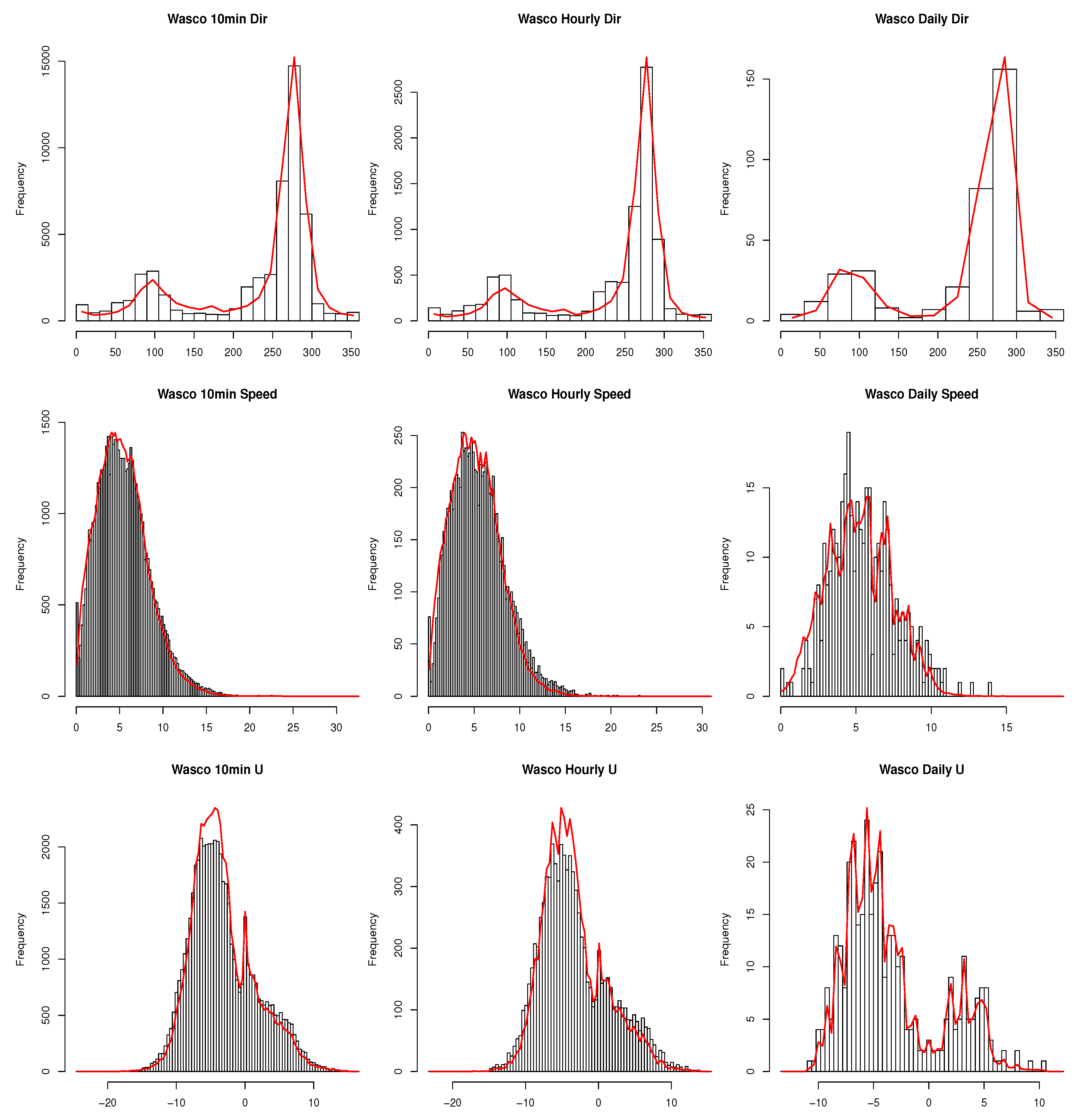
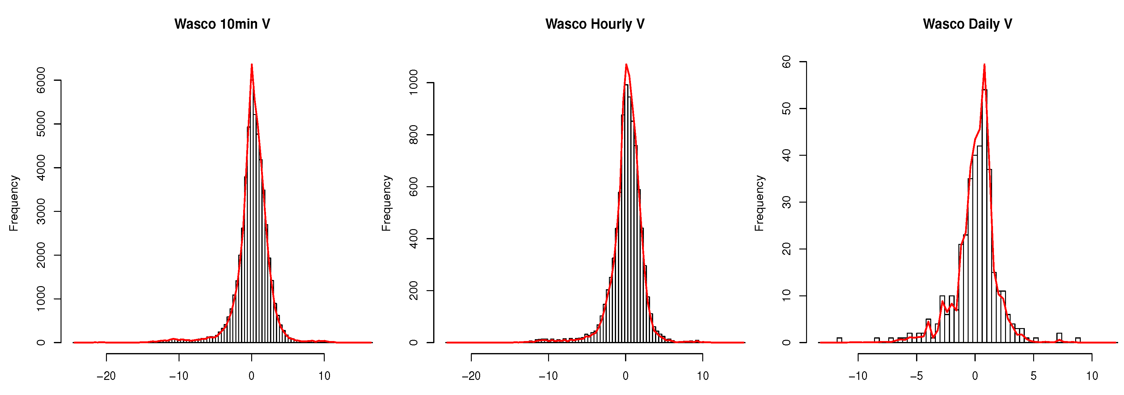
- the distribution of speed, direction, u and v;
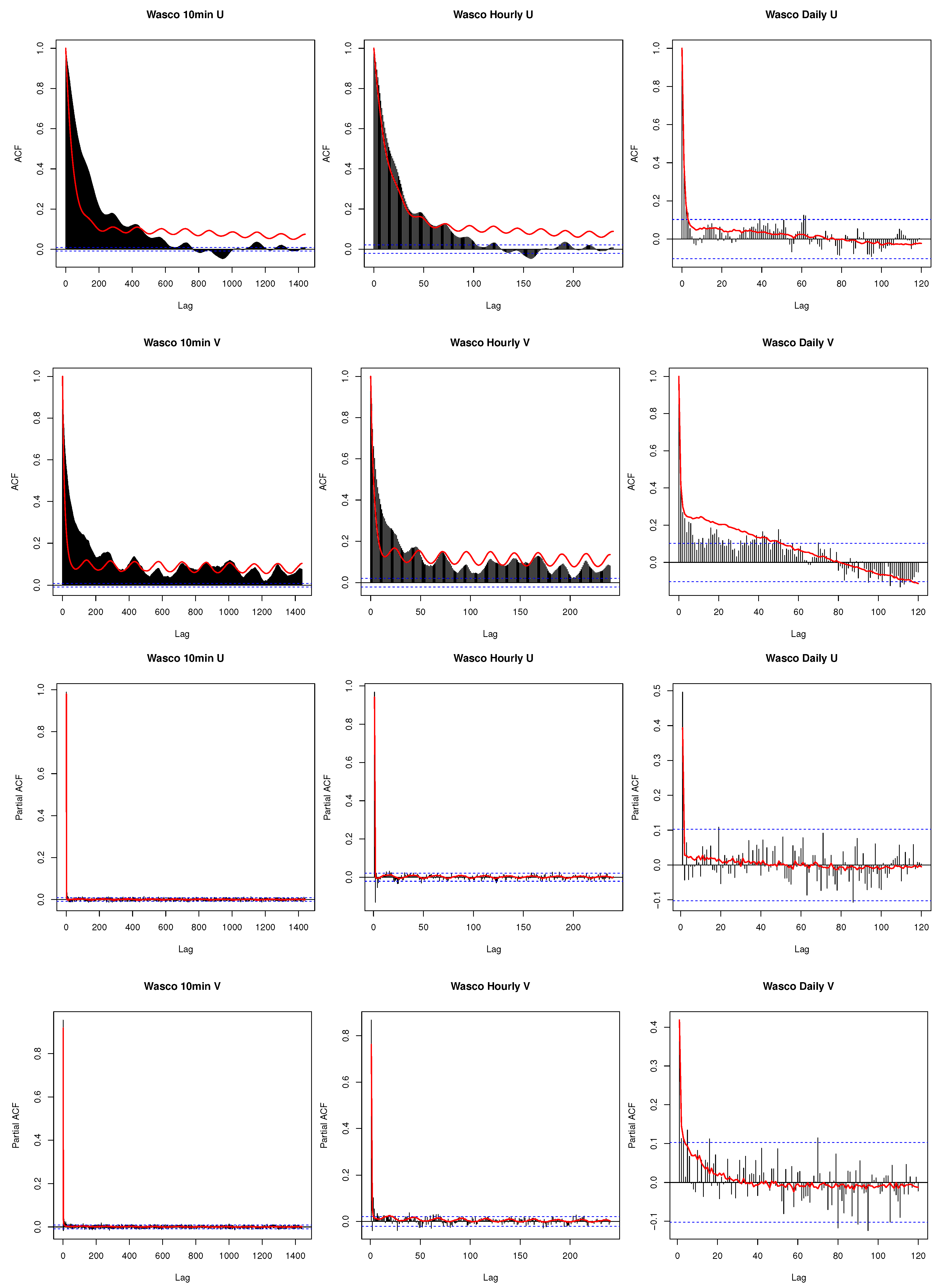
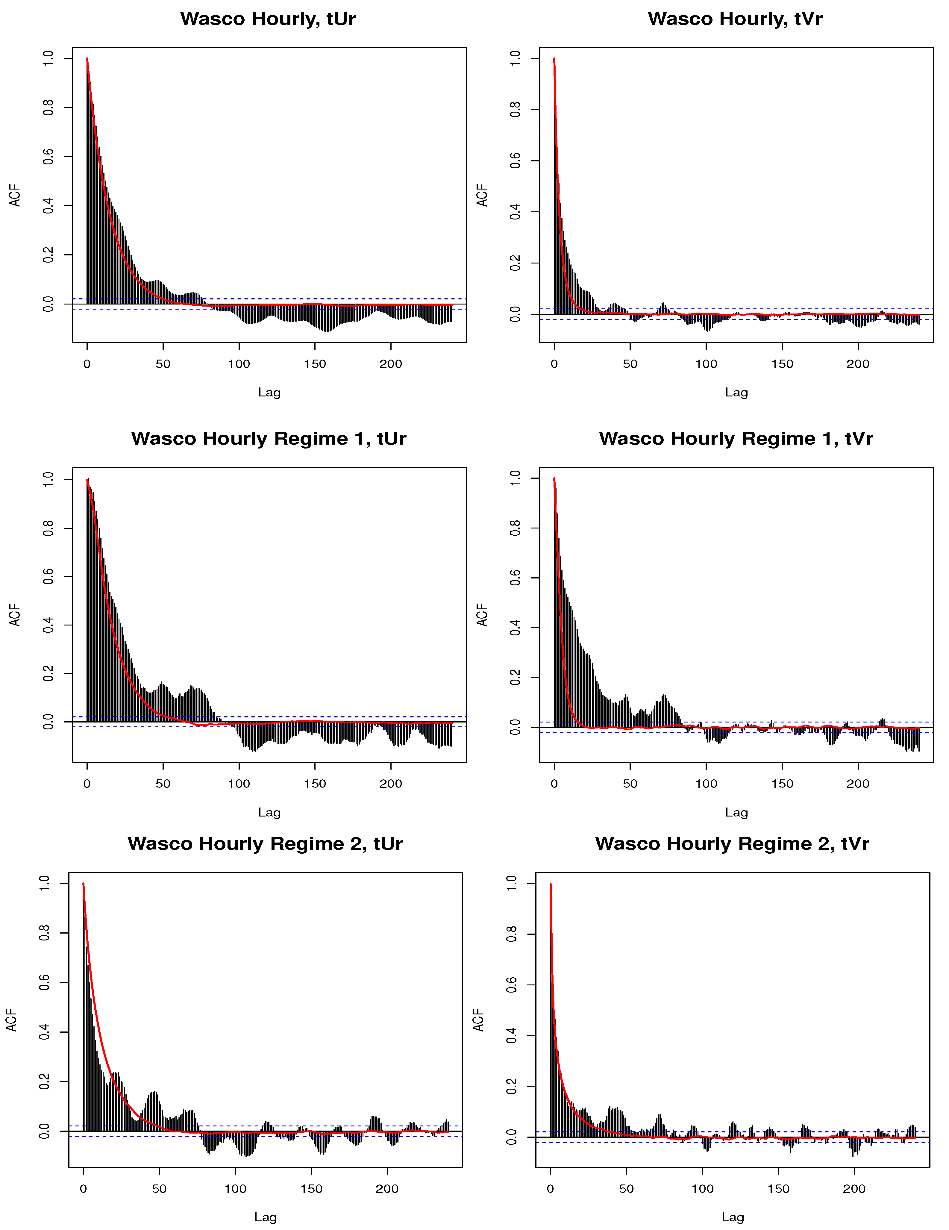
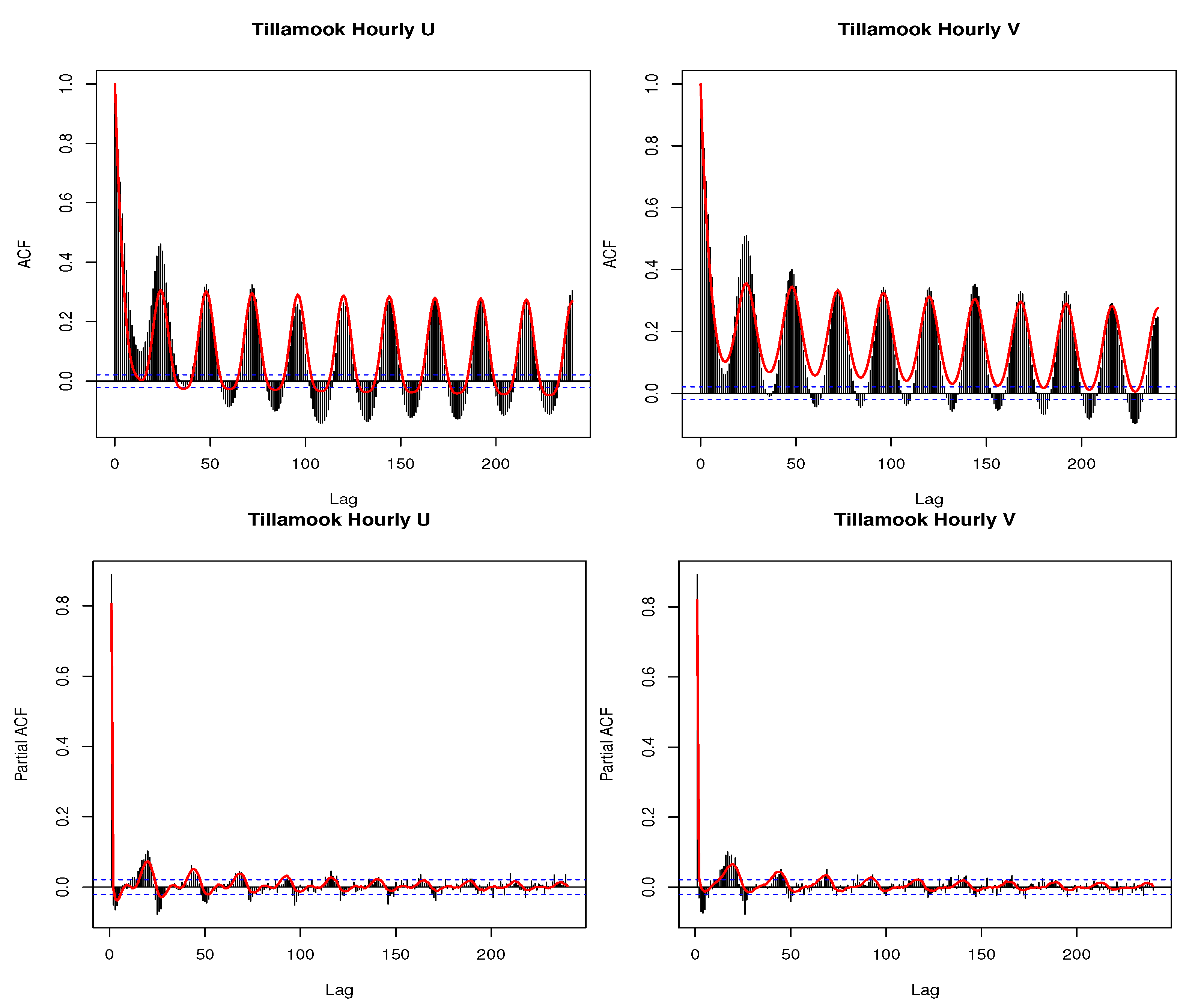
- the temporal autocorrelation of the u and v components;
- the diurnal variability of the u and v components;
- the joint distribution of speed and direction; and
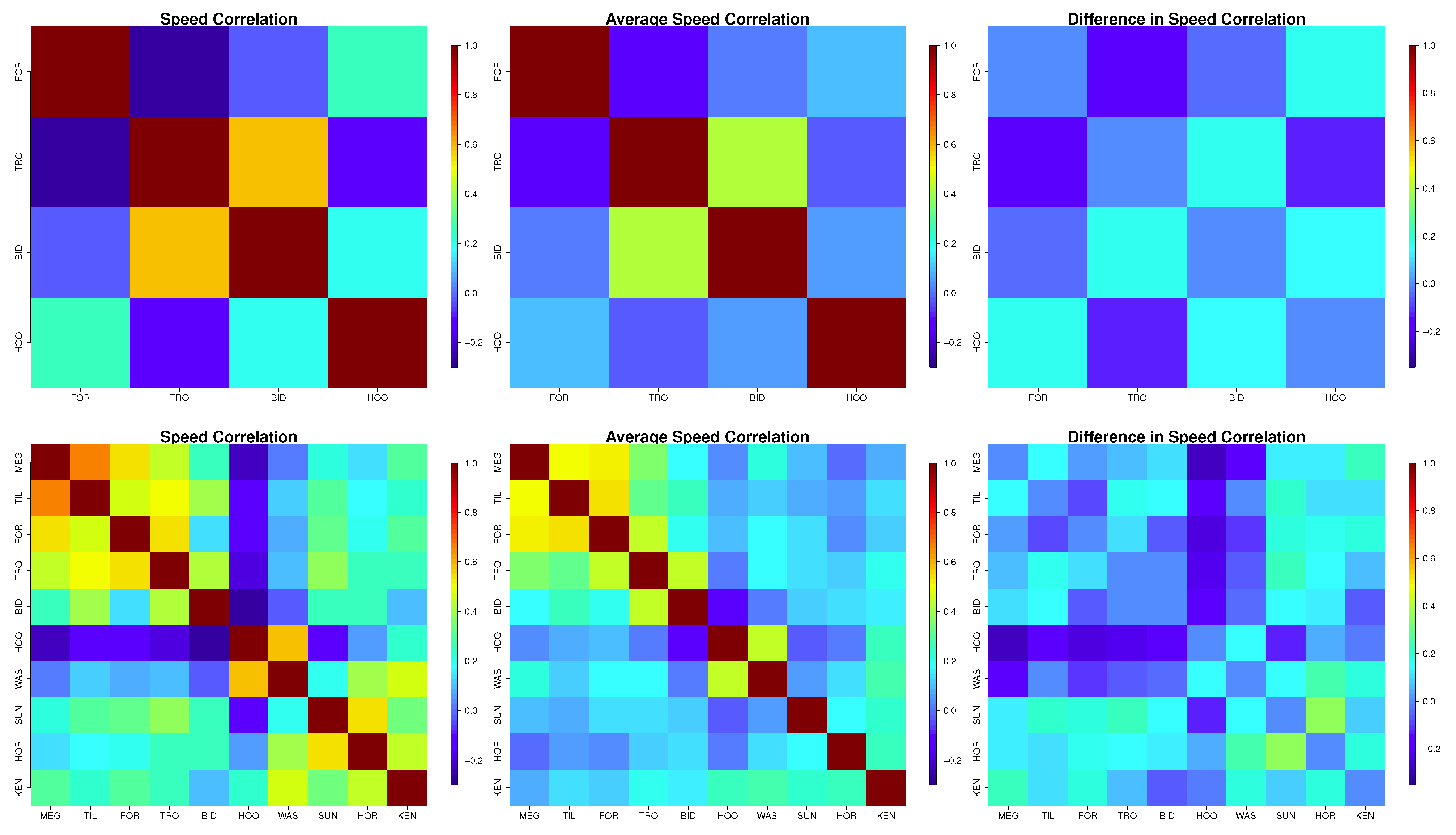
- the correlation between the u and v components.
- histograms of speed, direction, u and v of the observed data with the average count per bin taken across all 100 simulations overlaid;
- autocorrelation (ACF) and partial autocorrelation (PACF) plots of the observed u and v components with the average ACF and PACF for each lag taken over the 100 simulations overlaid (e.g., the average of 100 lag-1 autocorrelations is taken to obtain the plotted value), and diurnal variability can also be assessed with the ACF plots;
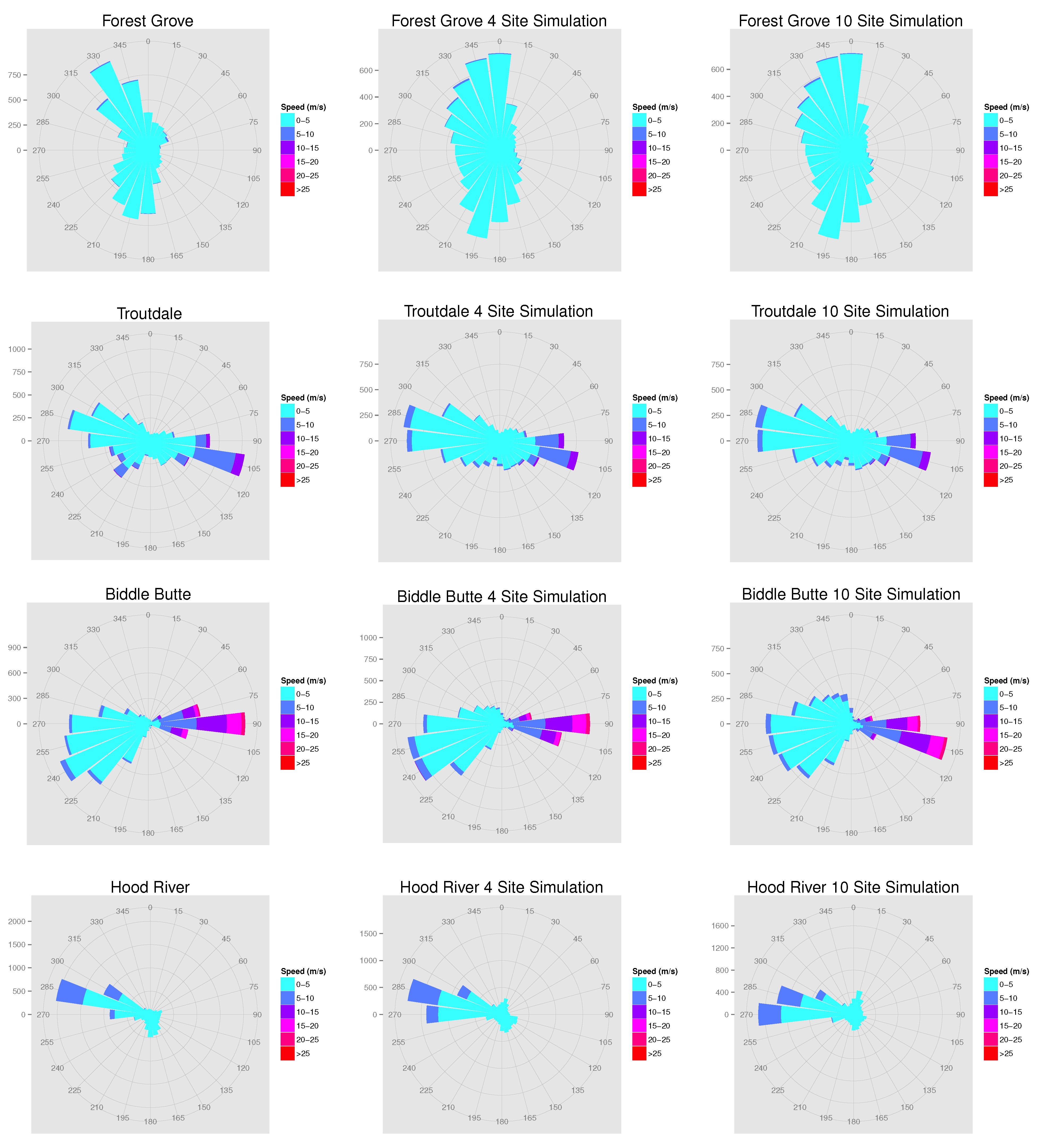
- wind roses of the observed speed and direction and wind roses of the average number of simulated observations across all 100 simulations occurring in each speed and direction bin;
- the observed correlation between the u and v components and the average correlation between the u and v components across all 100 simulations; and
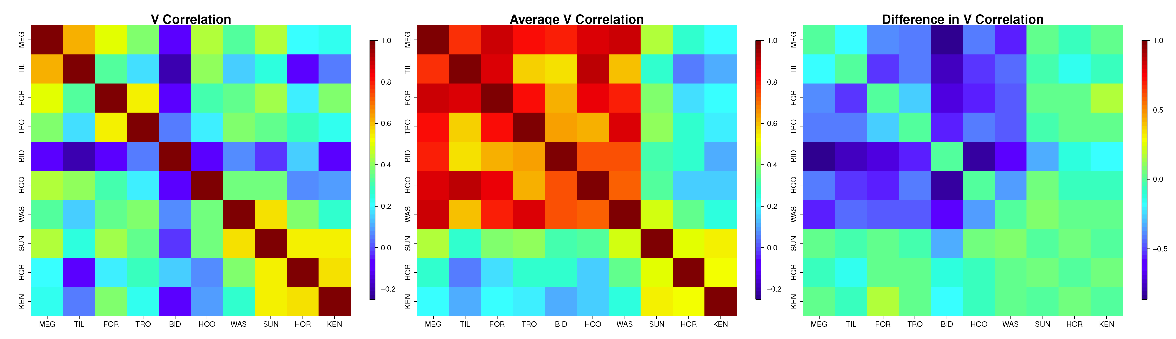
- a heat map of the spatial correlations among the observed u and v components and a heat map of the average of the spatial correlations across all 100 simulations.
4.1. Spatial and Temporal Scales


| Time Scale | ||||||||
|---|---|---|---|---|---|---|---|---|
| 10-min | 0.99 | 0.01 | 0.96 | −0.10 | 0.03 | 0.00 | 0.04 | −0.02 |
| 0.01 | 0.95 | 0.00 | 0.81 | 0.00 | 0.10 | −0.02 | 0.15 | |
| Hourly | 0.97 | 0.07 | 0.89 | −0.34 | 0.08 | 0.02 | 0.08 | −0.05 |
| 0.04 | 0.85 | −0.02 | 0.49 | 0.02 | 0.32 | −0.05 | 0.24 | |
| Daily | 0.36 | −0.07 | 0.61 | 0.47 | 0.62 | −0.08 | 0.80 | 0.49 |
| 0.03 | 0.19 | 0.28 | 0.46 | −0.08 | 0.49 | 0.49 | 0.70 | |

| Temporal | Spatial | Observed Overall Corr. | Simulated Overall Corr. |
|---|---|---|---|
| Tillamook | −0.37 | −0.42 | |
| Sunnyside | −0.03 | −0.17 | |
| Wasco | 0.02 | −0.23 | |
| 10-min | Coast | −0.11 | −0.10 |
| East | 0.55 | 0.42 | |
| West | 0.19 | 0.21 | |
| Region | 0.24 | 0.21 | |
| Tillamook | −0.39 | −0.47 | |
| Sunnyside | −0.01 | −0.28 | |
| Wasco | 0.02 | −0.30 | |
| Hourly | Coast | −0.10 | −0.09 |
| East | 0.56 | 0.42 | |
| West | 0.19 | 0.18 | |
| Region | 0.23 | 0.10 | |
| Tillamook | −0.25 | −0.14 | |
| Sunnyside | 0.19 | 0.15 | |
| Wasco | 0.14 | −0.13 | |
| Daily | Coast | −0.06 | −0.06 |
| East | 0.58 | 0.39 | |
| West | 0.21 | 0.05 | |
| Region | 0.28 | 0.40 |
4.2. Spatial Locations


5. Discussion
Author Contributions
Conflicts of Interest
References
- Skidmore, E.L.; Tatarko, J. Stochastic wind simulation for erosion modeling. Trans. ASAE 1990, 33, 1893–1899. [Google Scholar] [CrossRef]
- Reich, B.J.; Fuentes, M. A multivariate semiparametric Bayesian spatial modeling framework for hurricane surface wind fields. Ann. Appl. Stat. 2007, 1, 249–264. [Google Scholar] [CrossRef]
- Wikle, C.K.; Millif, R.F.; Nychka, D.; Berliner, L.M. Spatiotemporal hierarchical Bayesian modeling: Tropical ocean surface winds. J. Am. Stat. Assoc. 2001, 96, 382–397. [Google Scholar] [CrossRef]
- Fatichi, S.; Ivanov, V.; Caporali, E. Simulation of future climate scenarios with a weather generator. Adv. Water Resour. 2011, 34, 448–467. [Google Scholar] [CrossRef]
- Monbet, V.; Ailliot, P.; Prevosto, M. Survey of stochastic models for wind and sea state time series. Probab. Eng. Mech. 2007, 22, 113–126. [Google Scholar] [CrossRef]
- Masala, G. Wind time series simulation with underlying semi-Markov model: An application to weather derivatives. J. Stat. Manag. Syst. 2014, 17, 285–300. [Google Scholar] [CrossRef]
- Raischel, F.; Scholz, T.; Lopes, V.V.; Lind, P.G. Uncovering wind turbine properties through two-dimensional stochastic modeling of wind dynamics. Phys. Rev. E 2013, 88, 1–12. [Google Scholar] [CrossRef]
- Yang, H.; Li, Y.; Lu, L.; Qi, R. First order multivariate Markov chain model for generating annual weather data for Hong Kong. Energy Build. 2011, 43, 2371–2377. [Google Scholar] [CrossRef]
- DeCesaro, J.; Porter, K. Wind Energy and Power System Operations: A Review of Wind Integration Studies to Date; Subcontract Report NREL/SR-550-47256; National Renewable Energy Laboratory: Golden, CO, USA, December 2009. [Google Scholar]
- Marquis, M.; Wilczak, J.; Ahlstrom, M.; Sharp, J.; Stern, A.; Smith, J.C.; Calvert, S. Forecasting the windto reach significant penetration levels of wind energy. Bull. Am. Meteorol. Soc. 2011, 92, 1159–1171. [Google Scholar] [CrossRef]
- Kiviluoma, J.; O’Malley, M.; Tuohy, A.; Meibom, P.; Milligan, M.; Lange, B.; Holttinen, H.; Gibescu, M. Impact of wind power on the unit commitment, operating reserves, and market design. In Proceedings of the 2011 IEEE Power and Energy Society General Meeting, San Diego, CA, USA, 24–29 July 2011; pp. 1–8.
- Lannoye, E.; Flynn, D.; O’Malley, M.J. The role of power system flexibility in generation planning. In Proceedings of the 2011 IEEE Power and Energy Society General Meeting, San Diego, CA, USA, 24–29 July 2011; pp. 1–6.
- Ortega-Vazquez, M.; Kirschen, D. Estimating the spinning reserve requirements in systems with significant wind power generation penetration. IEEE Trans. Power Syst. 2009, 24, 114–123. [Google Scholar] [CrossRef]
- Zhu, X.; Genton, M.G. Short-term wind speed forecasting for power system operations. Int. Stat. Rev. 2012, 80, 2–23. [Google Scholar] [CrossRef]
- Pinson, P. Wind energy: Forecasting challenges for its operational management. Stat. Sci. 2013, 28, 564–585. [Google Scholar] [CrossRef]
- Brown, B.G.; Katz, R.W.; Murphy, A.H. Time series models to simulate and forecast wind speed and wind power. J. Clim. Appl. Meteorol. 1984, 23, 1184–1195. [Google Scholar] [CrossRef]
- Gneiting, T.; Larson, K.; Westrick, K.; Genton, M.G.; Aldrich, E. Calibrated probabilistic forecasting at the stateline wind energy center. J. Am. Stat. Assoc. 2006, 101, 968–979. [Google Scholar] [CrossRef]
- Hering, A.S.; Genton, M.G. Powering up with space-time wind forecasting. J. Am. Stat. Assoc. 2010, 105, 92–104. [Google Scholar] [CrossRef]
- Jeon, J.; Taylor, J.W. Using conditional kernel density estimation for wind power density forecasting. J. Am. Stat. Assoc. 2012, 107, 66–79. [Google Scholar] [CrossRef] [Green Version]
- Pinson, P.; Madsen, H. Adaptive modelling and forecasting of offshore wind power fluctuations with Markov-switching autoregressive models. J. Forecast. 2012, 31, 281–313. [Google Scholar] [CrossRef]
- Wilks, D.S.; Wilby, R.L. The weather generation game: A review of stochastic weather models. Progress Phys. Geogr. 1999, 23, 329–357. [Google Scholar] [CrossRef]
- Richardson, C.W. Stochastic simulation of daily precipitation, temperature and solar radiation. Water Resour. Res. 1981, 17, 182–190. [Google Scholar] [CrossRef]
- Parlange, M.B.; Katz, R.W. An extended version of the Richardson model for simulating daily weather variables. J. Appl. Meteorol. 2000, 39, 610–622. [Google Scholar] [CrossRef]
- Ivanov, V.Y.; Bras, R.L.; Curtis, D.C. A weather generator for hydrological, ecological, and agricultural applications. Water Resour. Res. 2007, 43. [Google Scholar] [CrossRef]
- Tan, K.; Chiew, F.H.S.; Grayson, R.B. Stochastic event-based approach to generate concurrent hourly mean sea level pressure and wind sequences for estuarine flood risk assessment. J. Hydrol. Eng. 2008, 13, 449–460. [Google Scholar] [CrossRef]
- Flecher, C.; Naveau, P.; Allard, D.; Brisson, N. A stochastic daily weather generator for skewed data. Water Resour. Res. 2010, 46. [Google Scholar] [CrossRef]
- Sahin, A.D.; Sen, Z. First-order Markov chain approach to wind speed modeling. J. Wind Eng. Ind. Aerodyn. 2001, 89, 263–269. [Google Scholar] [CrossRef]
- Shamshad, A.; Bawadi, M.A.; Wan Hussin, W.M.A.; Majid, T.A.; Sanusi, S.A.M. First and second orderMarkov chain models for synthetic generation of wind speed time series. Energy 2005, 30, 693–708. [Google Scholar] [CrossRef]
- Youcef Ettoumi, F.; Sauvageot, H.; Adane, A.E.H. Statistical bivariate modelling of wind using first-order Markov chain and Weibull distribution. Renew. Energy 2003, 28, 1787–1802. [Google Scholar] [CrossRef]
- Negra, N.B.; Holmstrøm, O.; Bak-Jensen, B.; Sørensen, P. Model of a synthetic wind speed time series generator. Wind Energy 2008, 11, 193–209. [Google Scholar] [CrossRef]
- Hocaoglu, F.O.; Gerek, O.N.; Kurban, M. The effect of Markov chain state size for synthetic wind speed generation. In Proceedings of the 10th International Conference on Probabilistic Methods Applied to Power Systems, Rincon, Puerto Rico, 25–29 May 2008; pp. 1–4.
- Scholz, T.; Lopes, V.V.; Estanqueiro, A. A cyclic time-dependent Markov process to model daily patterns in wind turbine power production. Energy 2014, 67, 557–568. [Google Scholar] [CrossRef]
- Brokish, K.; Kirtley, J. Pitfalls of modeling wind power using Markov chains. In Proceedings of theIEEE/PES Power System Conference and Exposition, Seattle, WA, USA, 15–18 March 2009; pp. 1–6.
- D’Amico, G.; Petroni, F.; Prattico, F. First and second order semi-Markov chains for wind speed modeling. Phys. A: Stat. Mech. Appl. 2013, 392, 1194–1201. [Google Scholar] [CrossRef]
- Lopes, V.V.; Scholz, T.; Estanqueiro, A.; Novais, A.Q. On the use of Markov chain models for the analysis of wind power time-series. In Proceedings of the 2012 11th International Conference on Environment and Electrical Engineering (EEEIC), Venice, Italy, 18–25 May 2012; pp. 770–775.
- Ailliot, P.; Monbet, V. Markov-switching autoregressive models for wind time series. Environ. Modell. Softw. 2012, 30, 92–101. [Google Scholar] [CrossRef] [Green Version]
- Burlando, M.; Antonelli, M.; Ratto, C.F. Mesoscale wind climate analysis: Identification of anemological regions and wind regimes. Int. J. Climatol. 2008, 28, 629–641. [Google Scholar] [CrossRef]
- Kazor, K.; Hering, A.S. Assessing the performance of model-based clustering methods in multivariate time series with application to identifying regional wind regimes. Agric. Biol. Environ. Stat. 2015, in press. [Google Scholar]
- Haslett, J.; Raftery, A.E. Space-time modelling with long-memory dependence: Assessing Ireland’s wind power resource. J. R. Stat. Soc. Ser. C 1989, 38, 1–50. [Google Scholar] [CrossRef]
- Goic´, R.; Krstulovic´, J.; Jakus, D. Simulation of aggregate wind farm short-term production variations. Renew. Energy 2010, 35, 2602–2609. [Google Scholar] [CrossRef]
- Ailliot, P.; Monbet, V.; Prevosto, M. An autoregressive model with time-varying coefficients for wind fields. Environmetrics 2006, 17, 107–117. [Google Scholar] [CrossRef]
- Bessac, J.; Ailliot, P.; Monbet, M. Gaussian linear state-space model for wind fields in the North-East Atlantic. Environmetrics 2015, 26, 29–38. [Google Scholar] [CrossRef] [Green Version]
- Hastie, T.; Tibshirani, R. Generalized Additive Models; CRC Press: Boca Raton, USA, 1990. [Google Scholar]
- Wood, S.N. Generalized Additive Models: An Introduction with R; Chapman and Hall/CRC: Boca Raton, FL, USA, 2006. [Google Scholar]
- Carapellucci, R.; Giordano, L. The effect of diurnal profile and seasonal wind regime on sizing grid-connected and off-grid wind power plants. Appl. Energy 2013, 107, 364–376. [Google Scholar] [CrossRef]
- Suomalainen, K.; Silva, C.A.; Ferrão, P.; Connors, S. Synthetic wind speed scenarios including diurnal effects: Implications for wind power dimensioning. Energy 2012, 37, 41–50. [Google Scholar] [CrossRef]
- Mardia, K.V.; Jupp, P.E. Directional Statistics; Wiley: New York, NY, USA, 1999. [Google Scholar]
- Fraley, C.; Raftery, A.E. Model-based clustering, discriminant analysis, and density estimation. J. Am. Stat. Assoc. 2002, 97, 611–631. [Google Scholar] [CrossRef]
- Fraley, C.; Raftery, A.E.; Murphy, T.B.; Scrucca, L. Mclust Version 4 for R: Normal Mixture Modeling for Model-Mased Clustering, Classification, and Density Estimation; Technical Report No. 597; Department of Statistics, University of Washington: Washington, DC, USA, 2012. [Google Scholar]
- Bonneville Power Administration Meteorological Weather Sites. Available online: http://transmission.bpa.gov/business/operations/wind/MetData.aspx (accessed on 11 February 2015).
- Yoder, M.; Hering, A.S.; Navidi, W.C.; Larson, K. Short-term forecasting of categorical changes in wind power with Markov chain models. Wind Energy 2014, 17, 1425–1439. [Google Scholar] [CrossRef]
- Zhu, X.; Genton, M.G.; Gu, Y.; Xie, L. Space-time wind speed forecasting for improved power system dispatch (with discussion and rejoinder). TEST 2014, 23, 1–25. [Google Scholar] [CrossRef]
- Azzalini, A.; Capitanio, A. Distributions generated by perturbation of symmetry with emphasis on a multivariate skew-t distribution. J. R. Stat. Soc. Ser. B 2003, 65, 367–389. [Google Scholar] [CrossRef]
© 2015 by the authors; licensee MDPI, Basel, Switzerland. This article is an open access article distributed under the terms and conditions of the Creative Commons Attribution license (http://creativecommons.org/licenses/by/4.0/).
Share and Cite
Hering, A.S.; Kazor, K.; Kleiber, W. A Markov-Switching Vector Autoregressive Stochastic Wind Generator for Multiple Spatial and Temporal Scales. Resources 2015, 4, 70-92. https://doi.org/10.3390/resources4010070
Hering AS, Kazor K, Kleiber W. A Markov-Switching Vector Autoregressive Stochastic Wind Generator for Multiple Spatial and Temporal Scales. Resources. 2015; 4(1):70-92. https://doi.org/10.3390/resources4010070
Chicago/Turabian StyleHering, Amanda S., Karen Kazor, and William Kleiber. 2015. "A Markov-Switching Vector Autoregressive Stochastic Wind Generator for Multiple Spatial and Temporal Scales" Resources 4, no. 1: 70-92. https://doi.org/10.3390/resources4010070