A New Approach for Optimizing Management of a Real Time Solar Charger Using the Firebase Platform Under Android

Abstract

With the continuous growth of energy consumption, the rationalization of energy has become a priority. The photovoltaic energy sector remains a major occupation for researchers in the field of production optimization or storage methods. The concept developed in this work is a mixed optimization approach for energy management during battery charging with a duty cycle. A selective collaborative algorithm intervenes to choose and use the appropriate results of the few techniques to optimize the charging time of a battery and estimate its state of charge by using the minimum possible tools. This is done using a collective database that is accessible in real time. It also effectively allows the synchronization of information between several customers. This approach is performed on a mobile application on android, through a Google Firebase platform that allows us to secure collaborative access between multiple customers and use the results of the calculations of some algorithms. It gives us the values obtained by the various sensors in real time to accelerate the charging speed of the battery. The validation of this approach led us to practice a few scenarios using an Arduino board to show that this approach has a better performance.

1. Introduction

Batteries, as energy storage elements, occupy a very important place in power generation facilities. The photovoltaic (PV) panel is one of the major sources of renewable energy used for recharging. The appearance of this source of energy further slows their development, because this storage is influenced by a few input parameters (source), such as the time of day, sunshine, solar radiation, and temperature. The non-linearity of a PV panel causes additional constraints and creates variables that make the overall system more complex.

The means of optimizing the recharging of a battery does not depend solely on the regulation device associated with it or the same types of batteries, but it is also directly related to the techniques employed in order to reach a maximum point of the necessary power [1]. These techniques are different, but the goal is always improving. As is the case with the authors of References [2,3], when it comes to a structure change, they deal with optimization problems using evolutionary strategies through self-adaptation as opposed to other authors who preferred, without any informatized interventions but with chemical enhancements [4,5], an adaptation between the photovoltaic source and the battery representing the load. Another particle swarm optimization process was addressed in References [6,7] by using multi-collinearity and using the stepwise method to control several numbers of parameters according to the battery terminals.

In other literatures, authors favor algorithms that rely on instantaneous measurements of voltage and currents across the battery, using programmable models or electronic components to estimate the SOC (State Of Charge). This is done by an extended Kalman filter in References [8,9]. In References [10,11], a group of researchers have thought as well about implementing a MPPT (Maximum Power Point Tracking) algorithm of a variable size incremental conductance method. The system of charge utilizes a method of constant voltage by a PI (Proportional Integral) controller that uses a genetic algorithm to determine the optimal gain.

A combination of some basic components, resistors, capacitors, and diodes allowed the authors of Reference [12] to achieve a modified Thevenin equivalent circuit model and treat nonlinearity to instantaneous variation as a linear model. Another model proposed by Reference [13] studies this optimization by the use of a Monte Carlo approximation of the SM (State-space model of Markov) algorithm with instantaneous sampling of the battery voltage and current magnitudes by the change of SM. The sensitivity of these quantities to the types of batteries as well as the value of the current of discharge was the problematic of Reference [14], whose authors used a network with radial basic function in order to increase the robustness of the algorithm.

Other types of controllers have a proprietary algorithm. This regulator takes into account the current that arrives and leaves the battery to permanently refine the visibility on its state of charge. The proprietary algorithm is self-learning in References [15,16] to have a good basis on the battery characteristics (age, capacity, etc.) after a number of cycles and thus optimize the load.

A presentation process was pursued in this document to connect the soft part to the hard part. The help provided to the device by the Firebase platform is illustrated through an android application. We started with the first section, where we show that there is a similarity between the research work that focuses on the detection of the state of charge of a battery. A new collaborative technique was also discussed, recruiting a new way to take advantage of remotely delivered enhancements by clouds such as Google’s Firebase Platform. Accordingly, any MPPT algorithm will benefit from the learning ability, which will offer a shorter computing time and a faster recharge. The regulation technique pursued as well as the detail of the overall system proposed with its electronic part takes place in Section 3 and Section 4 respectively. Section 5 explains the working method and operation of the Firebase platform through an android application and clarifies its positive effect on our device. Section 6 shows the location of the client sub-algorithms in the global algorithm as well as the influence of the collaboration on the initial value of the duty cycle that is to be used by the local map across the cloud. Knowing that the duty cycle represents the control input of the transistor, which is a priming angle; and is the method most used by electricians for commutation. To show the efficiency of our system as well as the algorithm pursued, we provide a series of experimental tests in the form of scenarios, the results are presented in a table in Section 7. The exact behavior of our algorithm is thus validated. This section is finalized by the explanation of the different reactions of the system, where the results appear as comparative figures. We focus on the performance of the collaborative algorithm and the gain reported by the global algorithm and the internal algorithm in two ways. Finally, we end our article with a general conclusion.

The main goal of this work is to take advantage of solar energy to accelerate the charging process of a battery by visualizing and monitoring the evolution of the voltage between its terminals as well as its state of charge. For that, a selective probabilistic algorithm with direct duty cycle control is implemented by designating the initial value of the duty cycle from a database accessible in real time using a Google Firebase platform. Officially, according to the primary values of the solar irradiation and the temperature measured by the local sensors, one finds the best value of the duty cycle which corresponds to the point of maximum power and is proposed to the converter by the system. The latter was previously calculated by another algorithm of a customer collaborating in this platform no matter what its optimization technique is. Whenever a new customer joins Firebase, automatically these input values as well as the optimization calculations by its algorithm are added to the databases and this increases the efficiency of our algorithm. That is why each collaborator will benefit from an initial optimization at the moment of his access to this platform if the conditions arise. In the case where there is no collaboration from the customers, from there, the database will be amplified according to the time elapsed. Since our recharging source is a solar panel, significant errors can occur due to poor selection of a duty cycle during a sudden climate change disrupting input parameters. Our algorithm converges quickly to the best duty cycle with an additional charging speed of 1.65% that can vary with the variation of the parameters of the database. This also allows to maintain the right MPP (maximum power point) as well as the right SOC; knowing that a SOC is good when it falls in a reasonable range which varies according to the battery. For example, the lithium battery falls into deep discharge when it reaches a level below 10% and a state of overload is reported when the level exceeds 100%; thus, its good SOC is situated between 40 and 95%. The simplicity of this algorithm allows us to take it as a real-time monitoring and analysis tool to diagnose batteries. The performance of this approach is related to the similarity of input parameters to ensure faster convergence at the MPP.

2. Similarities of Techniques and the Collaborative Methodology

The process of determining the SOC of a battery is always a problem that requires taking into consideration the temperature to perform a correct recharging [17,18,19]. This is specifically a requirement when the charging current is largely relative to the capacity of the battery which could lead to the overheating of the battery. Most chargers use the value of the voltage in determining the charging phase of the battery. However, it is important to note that this parameter is far from optimal to have an exact idea about the SOC of the battery. When the absorption voltage is reached, a timer is triggered to position the charger in float mode after a lapse of time. These types of chargers often give satisfactory results in the case where the maximum intensity is adapted to the battery park and when the latter two have a timer so that there is an actual absorption charge.

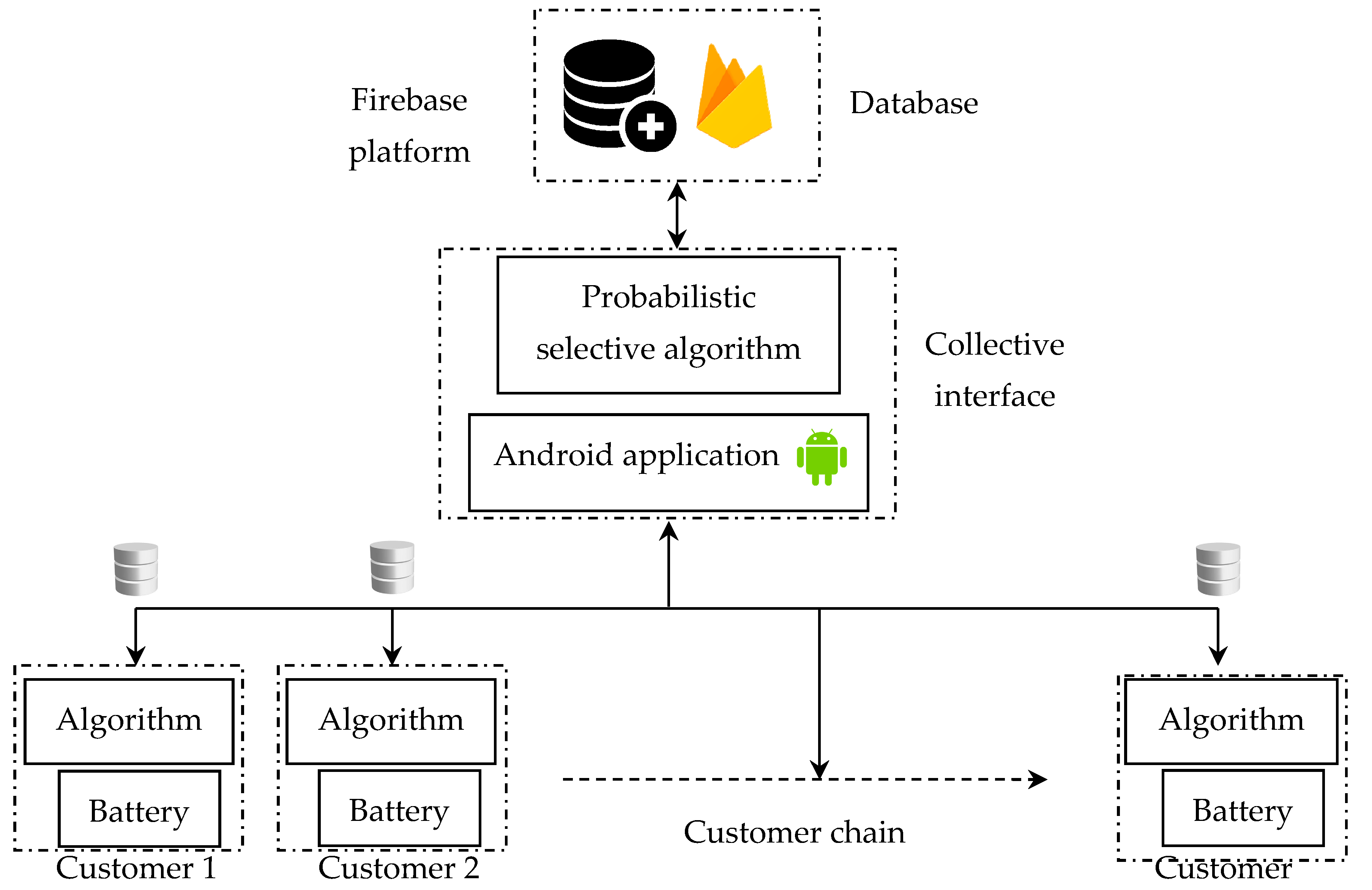
A collaborative approach is presented in Figure 1 which shows a general description of the appearance of our device. Each customer has his own optimization technique according to the charge controller which determines the SOC and the MPP if the battery is linked to a photovoltaic source. Therefore, the global variables of each system may be different in some parameters. Generally, the techniques used have a primary resemblance to what is essential (i.e., voltage, current and capacity of the battery, recharging phases of the battery, and the nature of the source of recharge).

Each customer participates with the calculation results of their algorithm to amplify the database under the Firebase platform of Google through an Android application; knowing that a customer represents any user seeking to charge a battery by means of a photovoltaic system as well as its local algorithm. The similarity of the input values is useful to optimize the recharge of the battery and to know its state periodically for each customer to facilitate an adaptation between them under this platform. The tool that allows to quickly reach the MPP and reduces the loading time is the probabilistic algorithm. Each client algorithm is associated with a parameter–result relationship and each system starts with a separate duty cycle after many calculations. The role of the probabilistic algorithm is to evaluate the performance of sub-algorithms under different operating conditions. The latter then associates the similarities and compares the different results to arrive at the best probability of making maximum profit from them by means of the most effective duty cycle. The client can therefore keep the results of his algorithm or select others that are more optimized.

Several problems confront the optimization in this sector and it is recommended to follow the recharge in three cycles for all types of battery. Depending on the technology used, a difference in the deterministic voltage values of the transition between the phases and the duration of the cycles must also be respected. During the first phase, called Bulk, the battery charges at a constant current. During this phase we require a maximum amount of power from our source which is reached through our MPPT technique. We also have to make sure that the battery is capable of receiving this maximum intensity (an eligible block).

During the second phase, the battery absorbs the energy with a constant voltage. It can be influenced by the value of the internal resistance which causes a greater intensity as well as the increase of the value of the temperature, which then leads to a shortening of the duration of this phase. Float is the last charging phase in which a voltage is applied very close to the battery voltage at rest. The latter is generally less than 14 Volts in order to fight against auto-discharge and produce energy of different consumers and keep the battery charged at the same time.

3. Regulation Technique

A procedure is taken into account only if the charge characteristic had to be the same depending on the type of battery, which forces us to create an adaptation of the regulator to the energy source no matter what its nature is. Thus, this poses no problem of the operation to a solar panel to put it in open circuit (without load). A wide range of solar controllers operate in PWM (Pulse Width Mode) mode [20,21] to comply with the charge states. The solar panel is brought into contact and is cut from the battery every 6.25 nanoseconds according to our regulator on the basis of the SOC of the battery (bulk, absorption or boost and floating). The battery then absorbs these impulses and regulates the voltage in the charge curve.

Another feature of our solar charge controller is that it supports the MPPT functionality, the solar panel can deliver the maximum of its power at a given voltage and current intensity depending on the temperature and the illumination while at the same time using a P&O (Perturb and Observe ) technique. The purpose of this type of regulator is to vary the input load to be at a MPP and it can offer a gain of approximately 25% energy compared to a standard regulator [22,23].

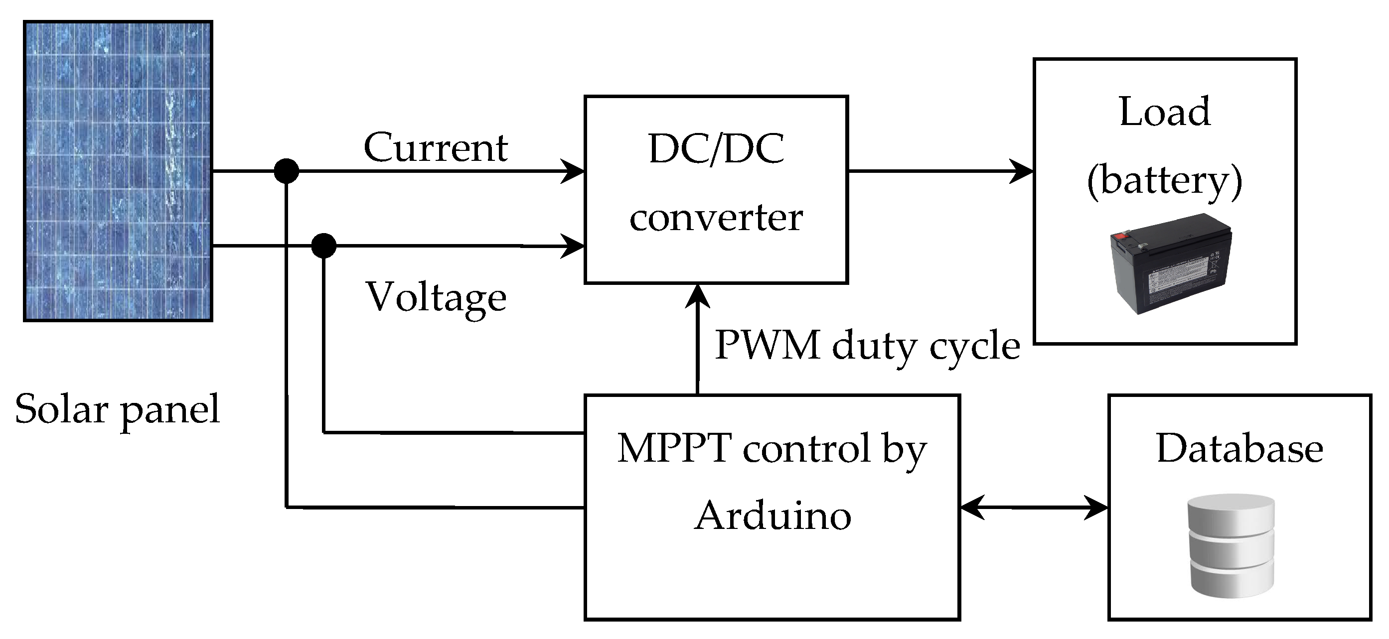
There may be a similarity in the optimization methods regardless of the algorithms or types of regulators used in our systems since the inputs and outputs are always identical at the parameter settings. Figure 2 englobes all the elements of the device.

According to Figure 2, the algorithm of control can generate a duty cycle or select it from the database according to the measures of current and tension to command the DC/DC converter and achieve a faster charging.

When it comes to a charging source such as photovoltaic panels, as it is in our case; there is a problem with the commissioning of the battery. However, the value of the initial battery state must be provided by the sensors using the Arduino board to ensure instantaneous monitoring and avoid an addition of new parameters unknown to the system. Most of the time, a deterministic voltage value set around 13.5 V requires battery charging by the power source and remains a flag if the panel is disconnected.

To model the characteristics of the PV (Photovoltaic) module, the electrical parameters of the solar module mentioned in

Table 1. Manufacturer specifications for a PV module.

Parameter	Value
Cell Type	Polycrystalline
Rated Power	10.0 (W)
Power Tolerance	±3%
Voltage at Maximum Power Vmp	17.5 (V)
Open Circuit Voltage Voc	21.5 (V)
Short Circuit Current Isc	0.56 (A)
Current at Maximum Power Imp	0.59 (A)
Dimensions	390 × 250 × 17 mm

are used. The converter is used in continuous conduction mode with the following calculated values: $f$ = 20 kHz, L = 25 mH, C = 73 μF.

In the IDE (Integrated Development Environment) of the Arduino we realized a main program which includes several macros corresponding to the different strategies used previously as well as the algorithm P&O.

Each manufacturer provides us with a graphical response that represents the characteristics and various charge evaluations to better control the battery overload, the power consumption compensation of the control system and the self-discharge. The atmospheric conditions directly affect the PV efficiency as well as the actual charging current that must be less than or equal to the maximum allowed current; the latter is limited by the Arduino board.

To calculate the values of the minimum and maximum voltage of the battery given on Equation (1) and to protect the battery against overheating, it is necessary to know some parameters that specify the battery according to the manufacturer. The model of the used battery is SLA−MS19V9 (12V9.0Ah), whose parameters are as follows:

• The minimum current is set to C/100
• The maximum current is set to C/5
• The charging current of the battery is set to I Trickle = 0.135A
• The maximum voltage of the battery is set at 14.8 V at 25 °C
• The minimum voltage is set at 13.6 V at 25 °C

Considering that "C" is the capacity of the battery in amperes-hours.

$$\{\begin{array}{c}{V}_{bat,\max }=14.8+\left(T_a-25\right)\times N_C\times \alpha \\ V_{bat,\min }=13.6+\left(T_a-25\right)\times N_C\times \alpha \end{array}$$

(1)

where Ta is the ambient temperature, N_C is the number of cells in the battery that is equal to 6 cells, α is the temperature compensation coefficient (its value is equal to −3.5 mV/C per cell) [24]. A few control actions are performed to regulate the charging process of the battery:

An adjustment pulse signal output from analog pin number 9 of the Arduino board is done to modify the duty cycle value according to the decisions made in the previous steps of the process. When the charging current of the battery requires a reduction, the duty cycle must be reduced as shown in Equation (2).

$$D_{k+1}=D_k-\left|\Delta D\right|$$

(2)

ΔD is the maximum accuracy allowed; it is resolved to 1/255 if the correction based on the Firebase database values is not improved. Another local process is triggered to activate the MPPT and the duty cycle adjusts as follows:

$$D_{k+1}=D_k+\left|\Delta D\right|\times sign\left(D_k\right)\times sign\left(P_{in,k}-P_{in,k-1}\right)$$

(3)

• $D_{k+1}$, $D_k$: correspond respectively to the values of the cyclic ratio of the iteration k + 1 and k in an interval of 0 to 255
• $\Delta D_k$: the duty cycle change value in step k is appropriate
• $P_{in,k}$, $P_{in,k-1}$: present the input power levels of the converter according to steps k and k − 1
• SIGN: is the sign added to the value according to Equation (3), it presents four computational probabilities

$$\{\begin{array}{c}if\begin{array}{cc}sign\begin{array}{cc}\left(D_k\right)>0& and\end{array}& \begin{array}{cc}sign\begin{array}{cc}\left(P_{in,k}-P_{in,k-1}\right)>0& \Rightarrow \end{array}& \Delta D\end{array}>0\end{array}\\ if\begin{array}{cc}sign\begin{array}{cc}\left(D_k\right)<0& and\end{array}& \begin{array}{cc}sign\begin{array}{cc}\left(P_{in,k}-P_{in,k-1}\right)<0& \Rightarrow \end{array}& \Delta D\end{array}>0\end{array}\\ if\begin{array}{cc}sign\begin{array}{cc}\left(D_k\right)>0& and\end{array}& \begin{array}{cc}sign\begin{array}{cc}\left(P_{in,k}-P_{in,k-1}\right)<0& \Rightarrow \end{array}& \Delta D\end{array}<0\end{array}\\ if\begin{array}{cc}sign\begin{array}{cc}\left(D_k\right)<0& and\end{array}& \begin{array}{cc}sign\begin{array}{cc}\left(P_{in,k}-P_{in,k-1}\right)>0& \Rightarrow \end{array}& \Delta D\end{array}<0\end{array}\end{array}$$

(4)

Equation (5) shows the connection between the converter input and output voltage values and the duty cycle value of PWM pin number 9 under continuous conduction operation mode [24].

$$D=\frac{V_{out}}{V_{in}}$$

(5)

$$\frac{dD}{d{V}_{in}}=-\frac{V_{out}}{V_{in}}<0$$

(6)

$V_{in}$ is the level of the input voltage of the converter and $V_{out}$ is that of its output. When there is a discontinuity of operation of our converter, we can write:

$$\frac{V_{out}}{V_{in}}=\frac{D^2}{D^2+\frac{I_{in}}{I_{LB,\max }}}$$

(7)

where:

$$I_{LB,\max }=\frac{V_{out}}{2\times f\times L}$$

(8)

$I_{in}$ presents the input current of the converter, L is the value of the inductance used and $f$ is the switching frequency. After some modifications on Equation (7) we find:

$$D=\sqrt{\frac{V_{out}\times I_{in}}{\left(V_{in}-V_{out}\right)\times I_{LB,\max }}}$$

(9)

According to the requirements of our algorithm, the successive decrease in the value of the duty cycle D leads the converter to regulate the charge current of the battery for a value lower than the maximum current. On the other hand, during the regulation process, there is a temporary increase in the duty cycle which does not cause any overload of the battery since the frequency of execution of the program is very high compared to the time constants of the battery.

4. The Proposed Global System

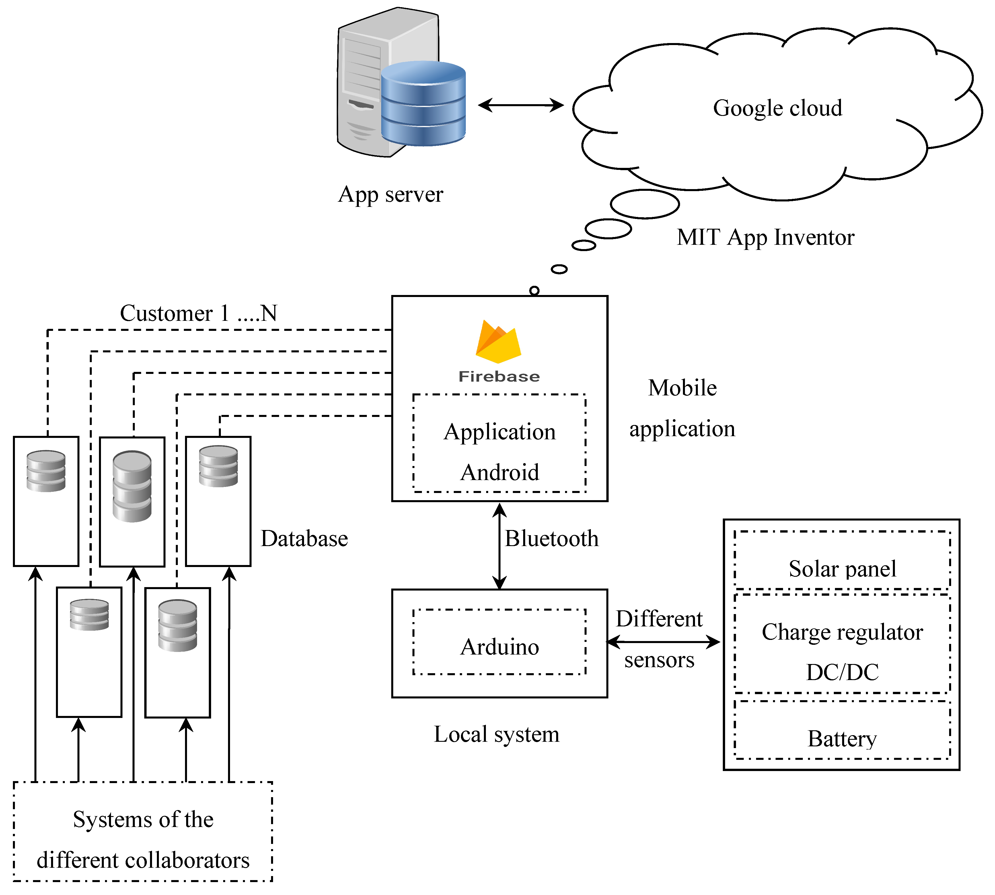
In Figure 3, a synoptic diagram presents the details of the proposed system; a step-down DC/DC converter is designed according to the requirements of the capacity of a photovoltaic source characterized in Table 1, a core of an Arduino Uno board which is an ATMEL microcontroller ATMega328 controls the interface circuits needed to manage the different sensors.

The control by a rectangular signal of the PWM (Pulse Width Modulation) type through the digital pin 9 of the Arduino board varies the duty cycle which represents the ratio between the conduction time and the total switching period. During its operations, the MOSFET turns on and off until the peak power point of the PV (photovoltaic panel) is reached where a local algorithm is implemented as a test title named P&O (Perturb and Observe) [20,21,22] to power a 12 V lead acid battery. Control and monitoring units are powered by the battery which is charged by the DC/DC converter. The voltage generated by the panel is measured by means of a voltage divider module on the analog bronchus 0. Another module named ACS712, mounted on the analog pin 1, presents the current sensor that measures the current delivered by the panel that can support up to 30 amperes. On the battery terminals, a previously mentioned voltage sensor is linked to the analog pin 2 of the Arduino board to provide us with the SOC at any time and another ACS712 connected to the analog pin 3 to measure the current coming out of the battery if it is linked to the charge. To monitor the ambient temperature of the battery, a DHT type sensor 22 is linked to the analog pin 4. The set of variables given by the units of measurement are displayed on a 84 × 48 LCD (Liquid Crystal Display) Nokia 5110 and a smart-phone screen by our application to inform the user about the slightest fluctuations and the various parameters of the system operation. This communication is done using a Bluetooth module type HC06 under a serial protocol. To store the input and output parameters as well as the best duty cycles, our application is equipped with a control and processing mode under a Google Firebase platform; it is developed under the MIT environment of App Inventor. The latter presents the intermediary between the application of the Firebase server (the global database) and the different customers that collaborate in this system.

Any information sent by the microcontroller is encoded by a pulse frame that carries the identifiers of the local system. If the algorithm presents a desired optimization, our application sends all the data as a base on Firebase so that the other collaborators can benefit from these values.

5. The Positive Effects of the Cloud Functions of Firebase on the Local Devices

Since the early days of cloud computing, many platforms have emerged to provide users with easy access to remote information and to use resources that cannot be obtained on our own. Google Firebase is considered the best and most powerful platform today for the many features it offers in free access.

There is no need to manage and have a server created or upgraded, as the Firebase’s cloud functions automatically execute backend code in response to each event triggered by Firebase features and HTTPS requests that are emitted by our application under android. The latter is also responsible for displaying the local parameters measured in real time and ensuring coordination between the customers by associating the results of similar inputs. The results of each customer’s calculation as well as the values of these input parameters will be stored in Google’s cloud and will be recalled by our main algorithm for subsequent use. The required input parameters stored on the platform and displayed on the application are: The SOC, the battery voltage, the PWM percentage, the voltage, current and PV power, as well as the ambient temperature.

Our application can use the cloud functions in response to each customer’s events so that it is aware of recent data relevant to changing local variable states on its system. The cloud function gives total access with considerable speed and scalable power to select the best duty cycle values in the corresponding time possible at the slightest fluctuation of the input or output values of the system [25,26].

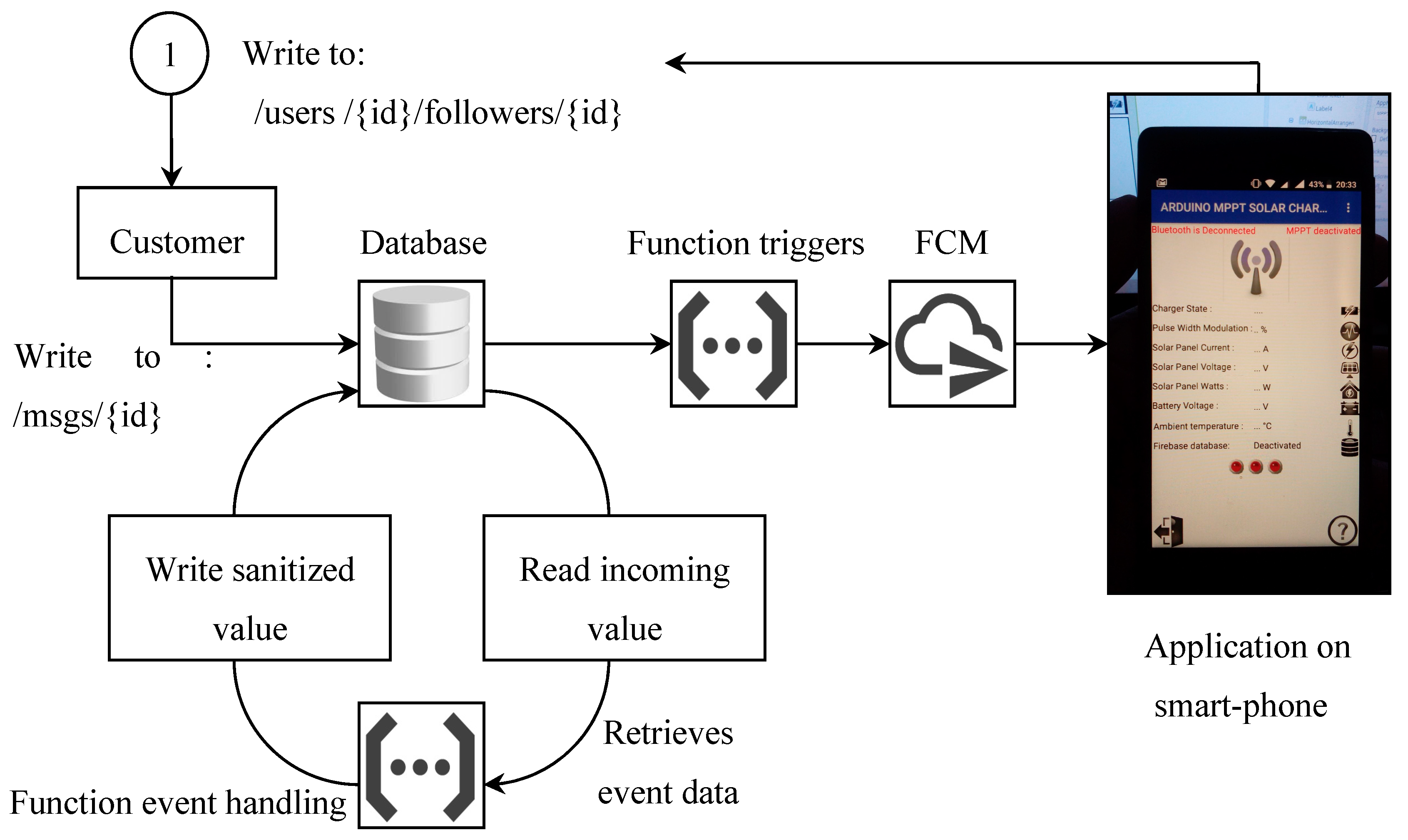
This task allows customers to track their activities as well as database variation using a triggering function that writes to the real-time database to store new optimization values; the approach of this task can be followed as follows:

• Event followers trigger (the function triggers) during the writing to the database path in real time to store new values.
• The function enters a message to send it by Firebase Cloud Messaging (FCM).
• FCM sends a notification message to the customer through the application to the devices.

The speed of execution of the algorithms of each customer when controlling the SOC of the battery is different following the optimization technique used and the number of inputs and outputs of the system as well as the electronic equipment used. As a result, it would not be practical to perform some intensive tasks on our own Arduino or microcontroller devices, since Google’s cloud computing provides us with resources and enormous power to compute and process data on the cloud in real time and with better synchronization between customers [27,28]. Figure 4 gives us a descriptive overview of the data processing by the application under the Firebase platform of Google.

A daily maintenance tightens to disinfect the database using cloud database event management functions by deleting unusable values that are marginalized or that have a slight probability of being used as optimal values for a given database collaborator. Hence, this answer is based on customer behavior towards optimal values.

6. Collaborative Algorithm

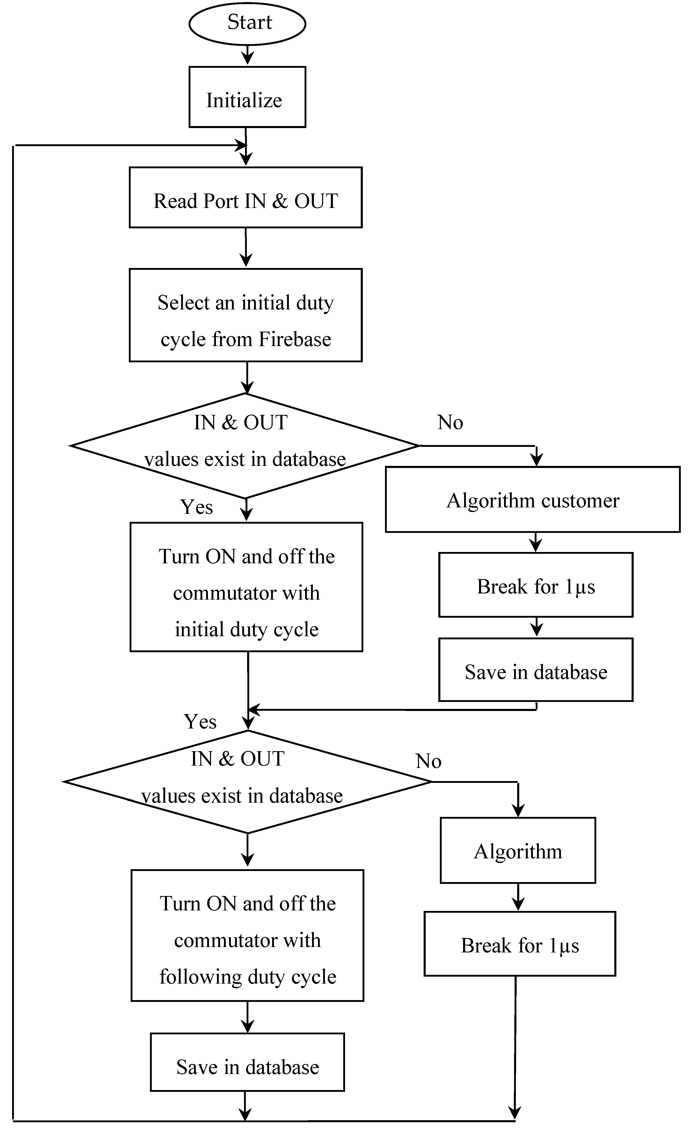
Figure 5 shows the essence of our algorithm which summarizes a priority procedure for the selection of an initial duty cycle after the initialization of the input and output variables of the system in order to accelerate the process of optimization of the MPP and the detection of the SOC of the battery.

The program flow illustrates the main loop that supports a switchover between two computational tasks based on the speed of data processing and the best results. The latter converge to the MPP of the source according to the voltage and current measurements from the solar panel and adequate states of charge delivered by reading and instantaneous monitoring of the voltage and the battery terminal current generating the best adopted duty cycle.

A timer is activated for a verification interruption if the input and output values already have an identical image on the Firebase platform saved by another customer or by the local user himself. A correction is sent to the system and the operation is followed by steps of adjustment of the duty cycle according to the decisions made by the collaborator who has the best convergence; if this correction carries an undesired divergence, the algorithm switches to the local correction and forces the system to work with its own algorithm but always taking into account a calculation in background for the values that approach the previously saved ones on the database so as not to get away from the best duty cycle.

According to our algorithm, some steps must be applied if the battery voltage is higher than the maximum voltage value. In other words, if it is in overload condition, the maximum current of the battery decreases.

Thus, at the next iteration of the algorithm, the present current of the battery will be reduced according to the previous control action. When the maximum battery current reaches C/100, which means that the battery is 100%, the maximum battery current is set to I trickle.

In particular, if the voltage of the battery does not reach the maximum voltage value, an interruption is triggered so that the duty cycle is set so as to maximize the PV output power (MPPT process or the selection of a value according to the database). In addition, if the battery voltage does not reach the minimum voltage value, which means a discharge state, the maximum charging current of the battery is adjusted to its initial value.

7. Experimental Trials and Validation of Results

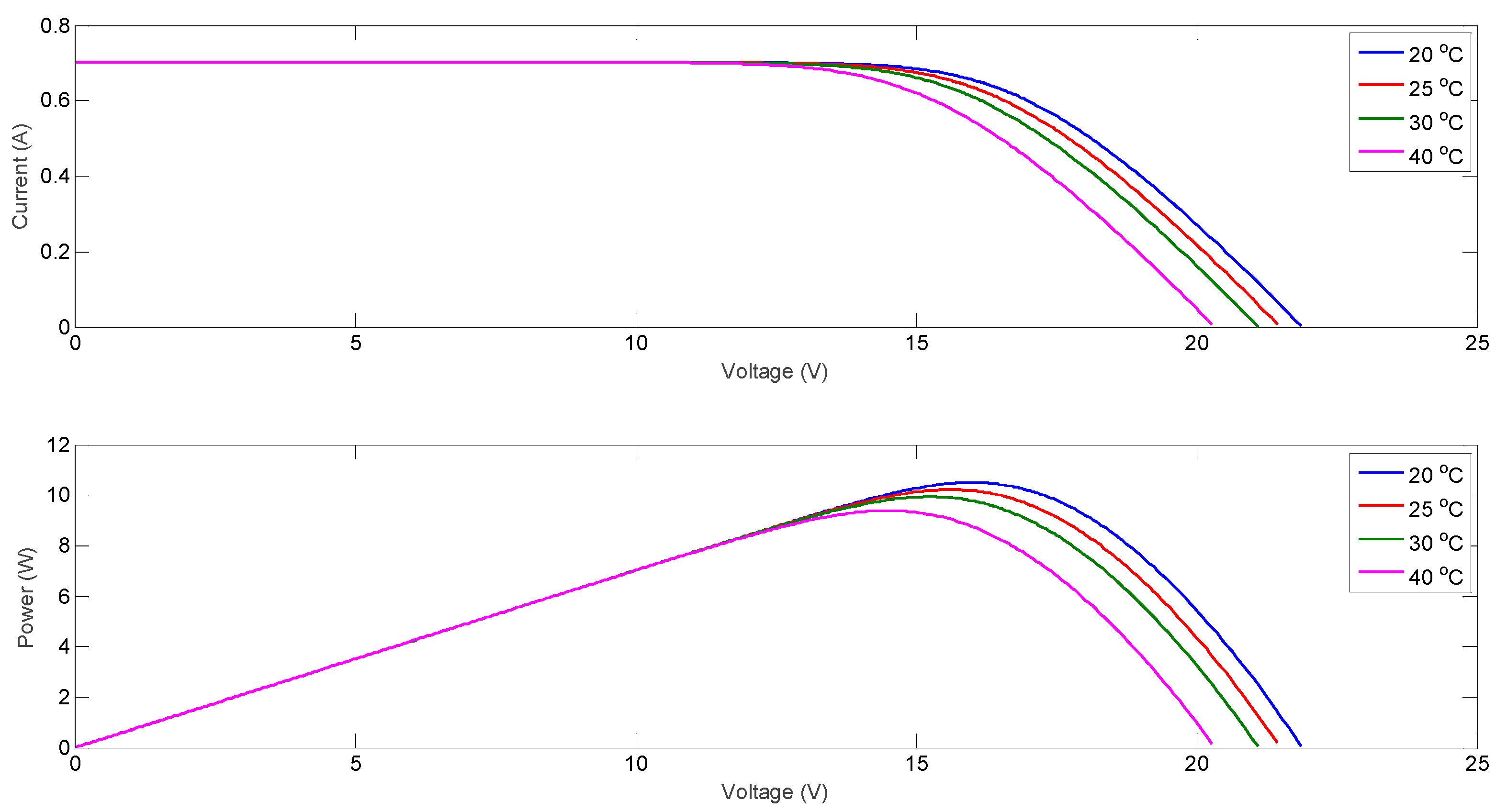
Before going to practice, we simulated our panel to diagnose the behavior of our source at the slightest fluctuations. The simulation of the solar panel has been carried out and verified as shown in Figure 6 and Figure 7 based on the electrical characteristics given by the manufacturer in the standard conditions (25 °C, 1000 W/m²) and some different levels of temperature and irradiation using the Matlab/Simulink environment.

Considering that the solar panel outputs are variable depending on the irradiation and the ambient temperature, the voltage across the battery will also depend on the SOC. We used potentiometers to get closer to reality and experimentation to realize three scenarios relating to the operation of the solar panel. Figure 8, Figure 9 and Figure 10 illustrate the simulation of these scenarios.

To show the influence and the intervention of the collaborative algorithm on the behavior of the system, an amplification of the Firebase database is executed with the flow of time by letting the system function without having recourse to an amplification through the optimization values of the few collaborators.

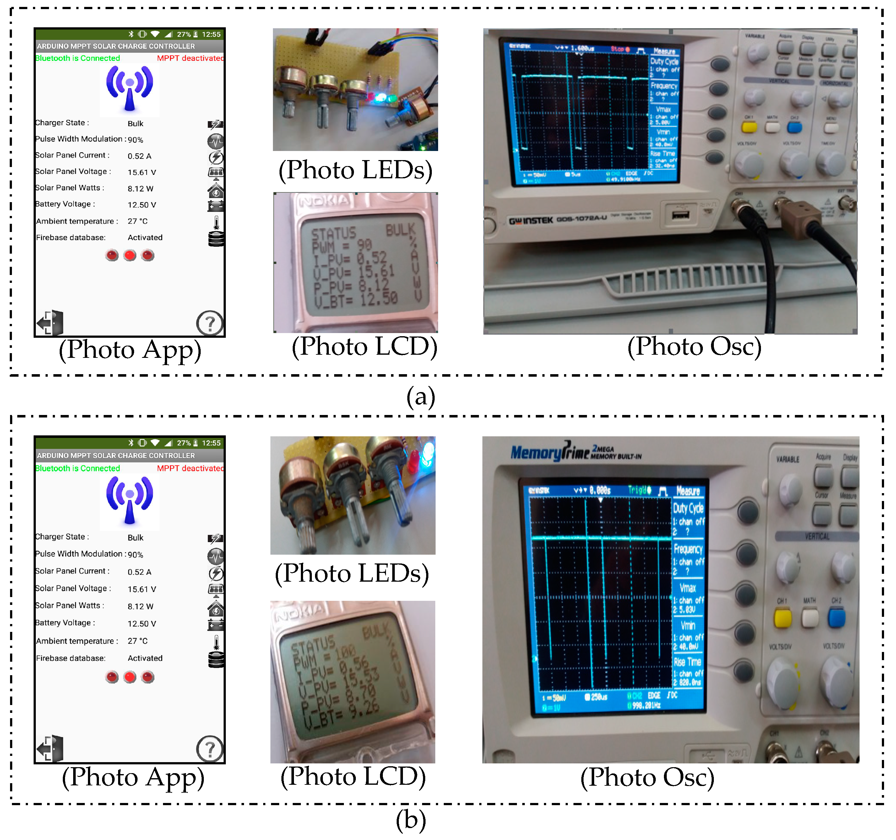
7.1. First Constant Temperature Scenario

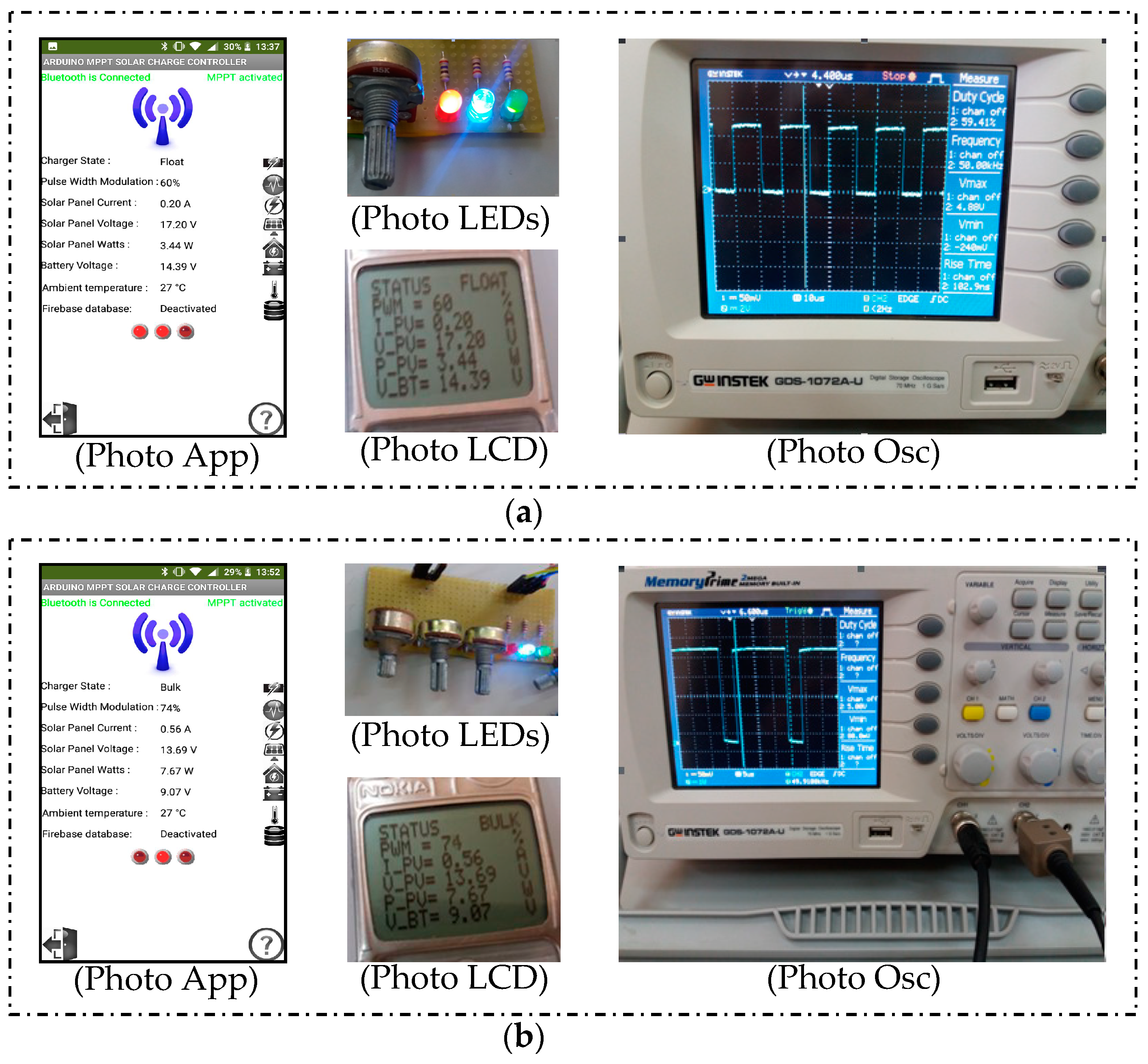
The temperature considered is 25 °C. Hence, the outgoing voltage of the solar panel is optimal, (17.55 V) while the illumination is variable. Therefore, the current obtained recedes from the optimal current given by the manufacturer of the panel, that is 0.56 A. By applying different voltages to the battery, we found that the SOC of the battery behaves according to the instructions of the program given to the indicator lights as well as the display of the quantities on the graphical interface of the application and our local display LCD. In Figure 8, some real photos were taken during the realization and all recorded data are shown in

Table 2. Answers and results of the first scenario.

VPV = 17.55 (V)
Battery Voltage (V)	Current of the PV (A)	Power of the PV (W)	Duty Cycle %	State of Charge	Label Indicator Light and Firebase Activation
<12	0.1 < I < 0.2	2.10	100	ON	OFF
	0.2 < I < 0.3	3.68	100	ON	OFF
	0.3 < I < 0.4	5.26	64	Bulk	OFF
	0.4 < I < 0.5	7.72	62	Bulk	OFF
	0.5 < I < Imax	8.95	60	Bulk	OFF
≈12	0.1 < I < 0.2	1.75	100	ON	OFF
	0.2 < I < 0.3	3.86	66	Bulk	OFF
	0.3 < I < 0.4	5.61	63	Bulk	OFF
	0.4 < I < 0.5	7.02	64	Bulk	OFF
	0.5 < I < Imax	9.65	60	Bulk	ON
≈14	0.1 < I < 0.2	1.93	100	Float	OFF
	0.2 < I < 0.3	5.12	65	Float	ON
	0.3 < I < 0.4	6.14	63	Float	ON
	0.4 < I < 0.5	7.30	62	Float	ON
	0.5 < I < Imax	9.40	60	Float	OFF
≈16	0.1 < I < 0.2	2.00	60	OFF	OFF
	0.2 < I < 0.3	3.69	60	OFF	ON
	0.3 < I < 0.4	6.14	60	OFF	OFF
	0.4 < I < 0.5	7.23	60	OFF	OFF
	0.5 < I < Imax	9.88	60	OFF	ON

, which we interpret.

In Figure 7, Figure 8 and Figure 9, we present real photos taken to explain the reaction of our system where: (Photo Osc) is the plot of the PWM on the oscilloscope, (Photo LEDs) present the potentiometers which are considered different input quantities as well as the three indicators that reveal the state of the converter, (Photo LCD) present the input values and the response of the system on a local LCD, same for the (Photo App) but on an application on a screen smart-phone. Where in each scenario, two samples were provided; the aim is to highlight the resemblance of the measured parameters.

On the global interface of our application a label indicates the values emitted by the database where we observe that there are only values that intervene by the algorithm after a certain moment, that is to say that the database increases with time. When the voltage value at the battery terminals is below 12 V and with the application of increasing current levels, we notice that the battery is in the charging start position, the green light is on and the power increases and the system puts the battery in Bulk position, where the latter charges itself quickly with the maximum power using the local algorithm as shown in the cells of the last column of the Table 2. The duty cycle changes with the increasing power generated by the panel. In the case where the value of the battery is greater than 12 V and less than 14 V, and applying the same variations of current, it is noted that when the power is minimal, the system applies a duty cycle equal to 100%.

With the increase of the power generated by the panel, the converter is in Bulk state with the introduction of the various duty cycle values from the Firebase database. When the battery level is adjacent superior to a value of 14 V, the increasing change in the current requires the duty cycle to be 100% for the minimum power values and varying when these values are more significant while maintaining the state float. This correction comes from the local algorithm and the collaborative algorithm as the label displays on our application.

At the end of Table 2, when the battery voltage is large, regardless of the current value, the system requires a fixed duty cycle equal to 60% to avoid overload and the system prepares to start another cycle if the level battery is degraded. That is with the optimization of the local algorithm and the Firebase optimization values.

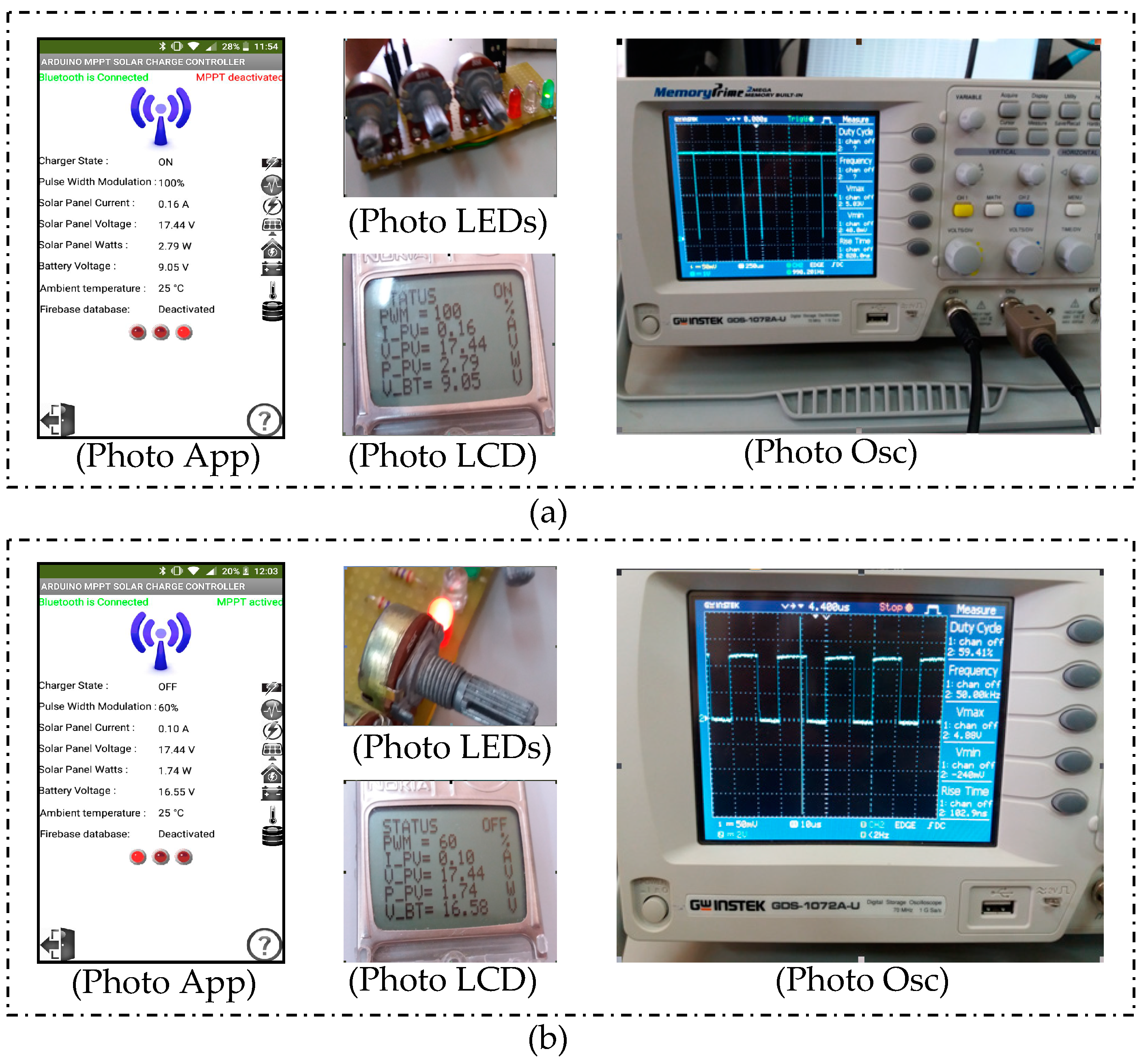
7.2. Second Constant Irradiation Scenario

The illumination considered is 1000 W/m², hence the current leaving the solar panel is optimal, or 0.56 A, while the temperature is variable. Therefore the voltage obtained recedes from the optimal voltage given by the manufacturer of the panel (17.5 V). By acting on the potentiometer that represents the variation of the voltage of the battery, we notice that the battery follows the logarithmic approach. In Figure 9, some real photos summarize the second scenario as well as some system responses and results in

Table 3. Answer and results of the second scenario.

IPV = 0.56 A
Battery Voltage (V)	Current of the PV (A)	Power of the PV (W)	Duty Cycle %	State of charge	label Indicator Light and Firebase Activation
<12	12 < V < 13	7.02	73	Bulk	OFF
	13 < V < 14	7.77	78	Bulk	ON
	14 < V < 15	7.96	80	Bulk	ON
	15 < V < 15.50	8.45	83	Bulk	ON
	V > 15.50	9.31	85	Bulk	OFF
>12	12 < V < 13	7.15	84	Bulk	OFF
	13 < V < 14	7.56	87	Bulk	OFF
	14 < V < 15	7.98	90	Bulk	OFF
	15 < V < 15.50	8.43	89	Bulk	ON
	V > 15.50	8.70	93	Bulk	ON
>14	12 <V < 13	6.98	60	Float	ON
	13 < V < 14	7.39	60	Float	OFF
	14 < V < 15	8.12	60	Float	OFF
	15 < V < 15.50	8.51	60	Float	OFF
	V > 15.50	8.70	60	Float	OFF

.

When the battery voltage approaches 12 V, higher or lower, regardless of the generated panel voltage, the duty cycle varies and the static converter is set to the Bulk state by the optimization values given by the collaborative algorithm and the local algorithm. In addition, if the battery voltage is higher than 14 Volts, the duty cycle is fixed at 60%, the algorithm continues its calculations when reaching the maximum voltage across the battery where all the LEDs light up, we say that it is in the Float position or end of the battery charge.

After that, part of the local algorithm and the collaborative algorithm ensure the protection of the battery by disconnecting the PV to avoid its overload and the indicator light is red.

7.3. Third Scenario Variation of Illumination and Temperature

Since the power of the panel depends on climatic variations such as temperature and irradiation, this scenario allows the adjustment of the two current voltage parameters deluded by the panel which are the image of the change in reality. This is caused by analog inputs of the Arduino board from the potentiometer. This procedure is random in order to better observe the response of our system. It is summarized in Figure 10 and

Table 4. Answer and results of the third scenario.

Battery Voltage (V)	Voltage and Current of the PV (V et A)	Power of the PV (W)	Duty Cycle %	State of Charge	Label Indicator Light and Firebase Activation
<12	(17.55 - 0.56)	9.82	83	Bulk	ON
	(12.20 - 0.30)	3.66	100	ON	ON
	(17.23 - 0.21)	3.61	100	ON	OFF
	(13.00 - 0.56)	7.28	76	Bulk	ON
	(12.55 - 0.56)	7.02	74	Bulk	OFF
≈12	(17.55 - 0.56)	9.82	99	Bulk	OFF
	(12.20 - 0.30)	3.66	100	ON	OFF
	(17.23 - 0.21)	3.61	100	ON	ON
	(13.00 - 0.56)	7.28	86	Bulk	ON
	(12.55 - 0.56)	7.02	84	Bulk	OFF
≈14	(17.55 - 0.56)	9.82	60	Float	ON
	(12.20 - 0.30)	3.66	60	Float	OFF
	(17.23 - 0.21)	3.61	60	Float	ON
	(13.00 - 0.56)	7.28	60	Float	OFF
	(12.55 - 0.56)	7.02	60	Float	OFF

.

At the application of an optimal voltage and current, the power obtained is sufficient for the battery to be in the Bulk position and the battery is rapidly charged with the maximum power; At the application of a low voltage and current, the power obtained is not sufficient for the battery to be in the Bulk position and the latter will be in the ON position with the stepwise running of the program until reaching the maximum voltage; at the application of a low voltage and an optimal current, the power obtained is sufficient for the battery to be in the Bulk position and the latter is charged quickly with the maximum power; at the application of an optimal voltage and a low current, the power obtained is not sufficient for the battery to be in the Bulk position and the latter will be in the ON position, with the stepwise running of the program until at reaching the maximum voltage. The algorithm continues its calculations until reaching the maximum voltage across the battery, all the indicator lights turn on, we say that it is in the Float position or the end of charging the battery. Subsequently, part of the program ensures the protection of the battery by its disconnection and the indicator light is red.

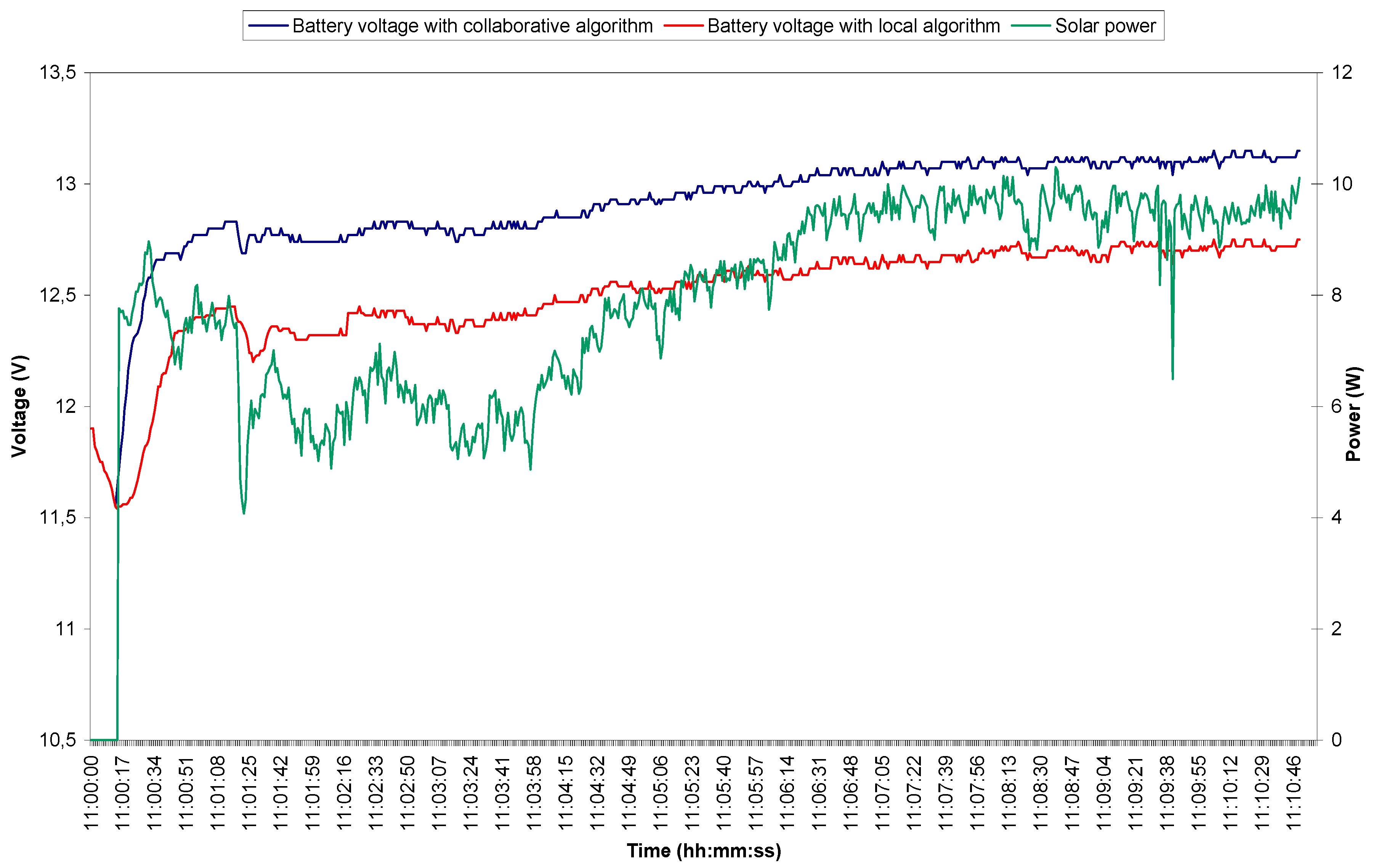
To reinforce our argument, we made a comparison concerning the behavior of the system with and without a collaborative algorithm extending in a short time interval on the same plane; as shown in Figure 11, where we find on the left y axis voltage values of the battery with and without the intervention of the collaborative algorithm. On the right y axis is the power generated at the same time.

In the first fifth seconds, the panel was put out of the system to observe the behavior of the battery. We note the same decrease in the voltage of the battery with and without a collaborative algorithm. After the exposure of the panel to irradiation, the drawing of the collaborative algorithm starts with optimal values due to the selection of an initial duty cycle, unlike the other battery which takes time to reach the maximum voltage during thirty-four seconds. We also note that during the rest of the experiment, the plot given by the system to the presence of the collaborative algorithm shows a profit which follows the values obtained from the Firebase database compared to the given plot when deactivating the collaborative algorithm where the local algorithm is the manager. During the slight, apparent weather disturbances on the power plot, the collaborative algorithm system exhibits a faster and more efficient stabilization than the other system during eight minutes and sixteen minutes. Moreover, the similarity between the two curves, without taking into account the difference in the benefit, demonstrates that the local algorithm works even during the activation of the collaborative algorithm and favors its results over those of the latter according to the performance and the values of the power given by the PV. To conclude, the curves show a lead of 1.65% over a period of 10 min which represents a voltage gain of about 0.4 V for the battery. That is in favor of the collaborative technique. This gain is not fixed but varies according to the input values and the amplification level of the database.

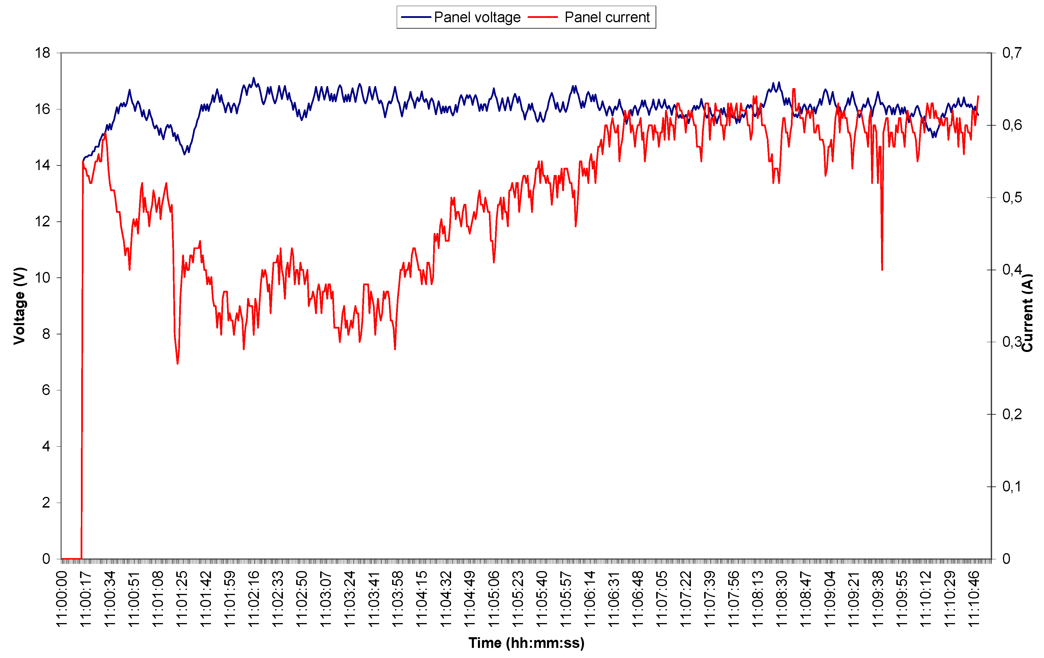
In order to track down the exact magnitude that has the most significant influence, Figure 12 is shown. It presents the voltage and current intensity generated by the panel simultaneously with Figure 11 where the shape of the current curve is strongly similar to the power curve shown in the previous Figure.

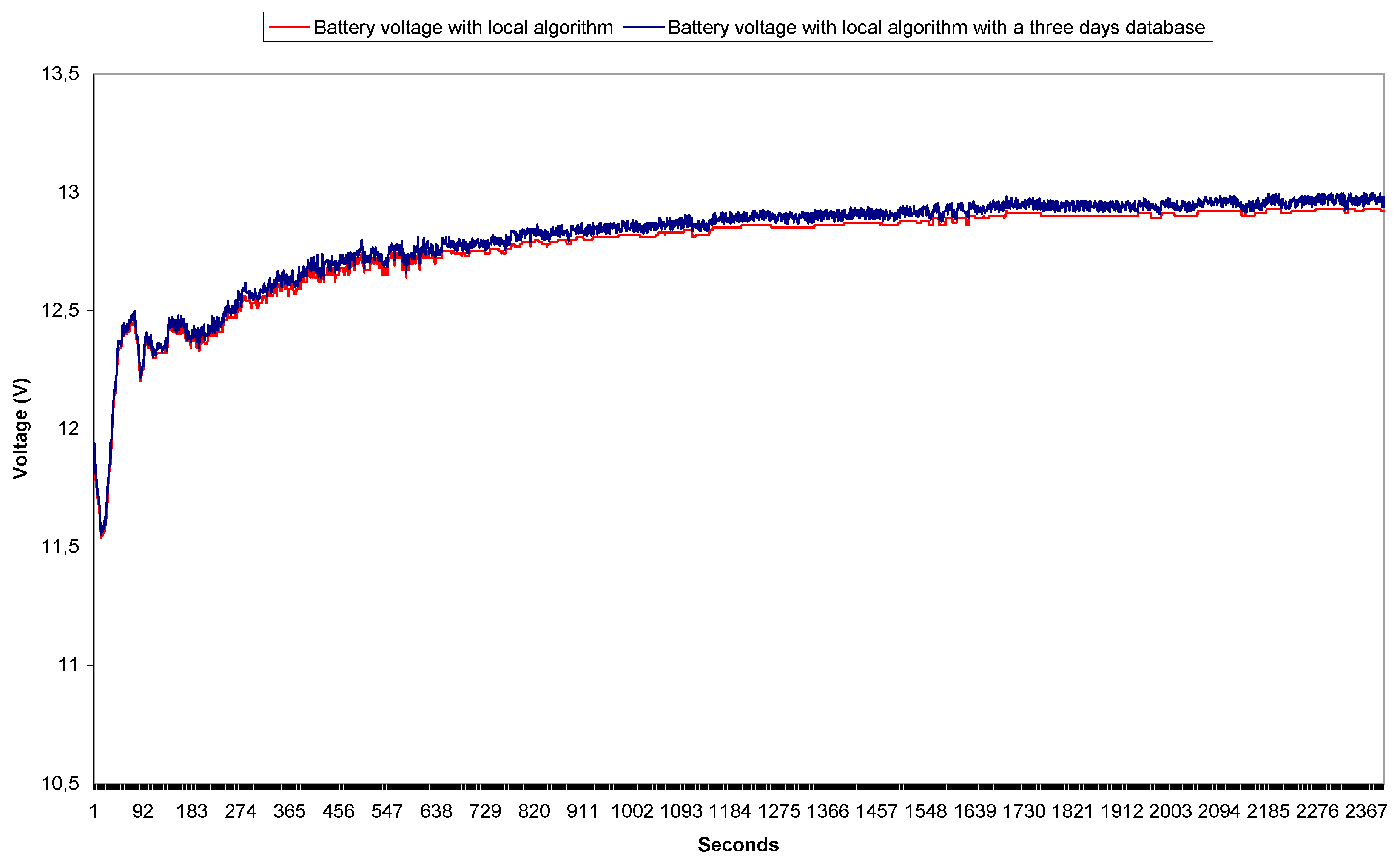
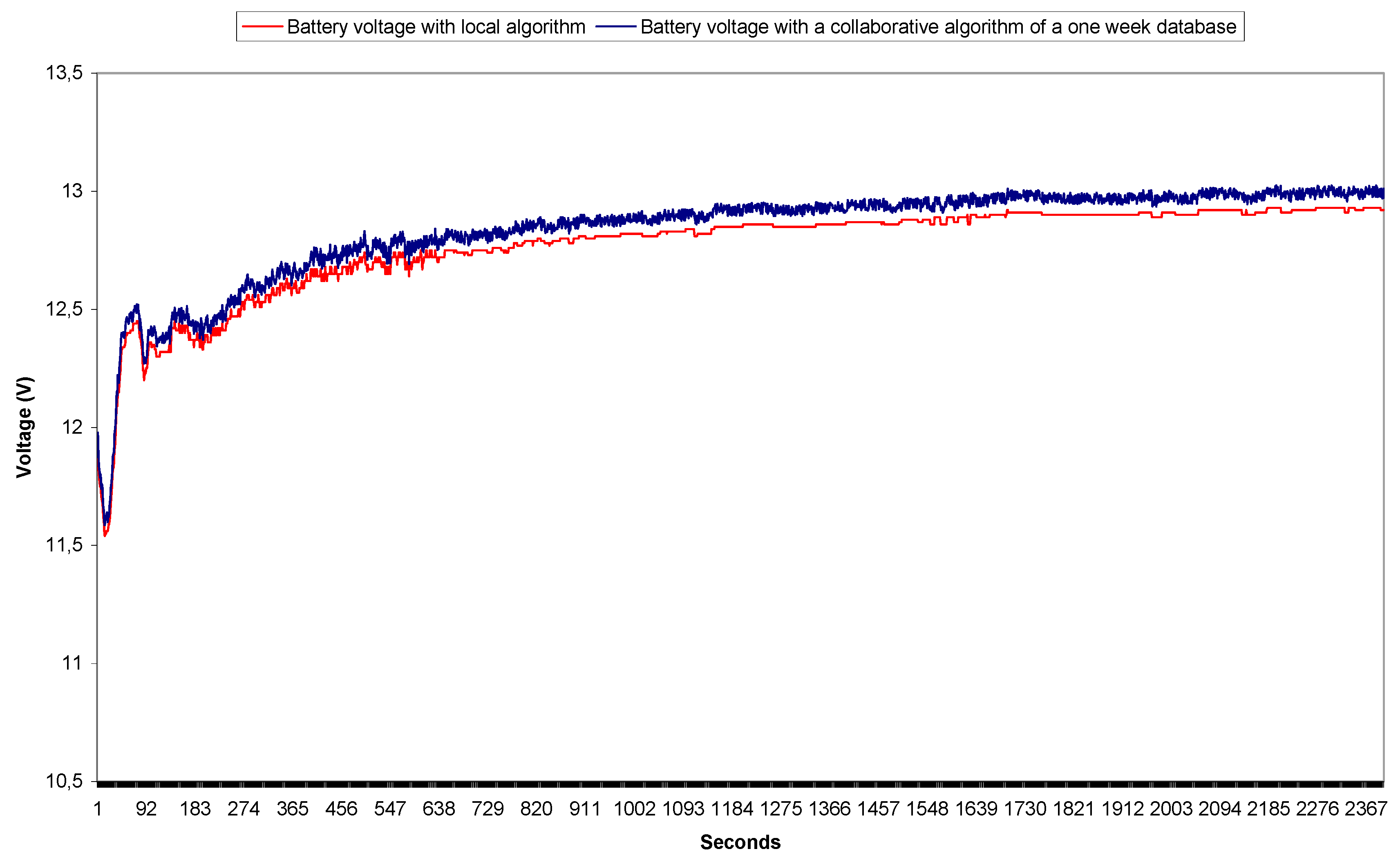
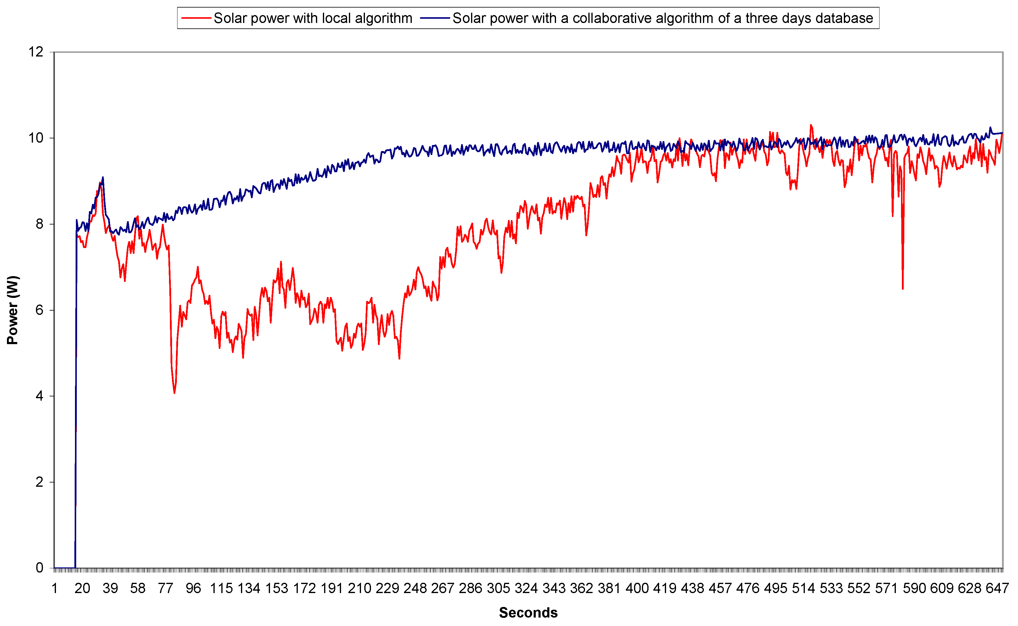
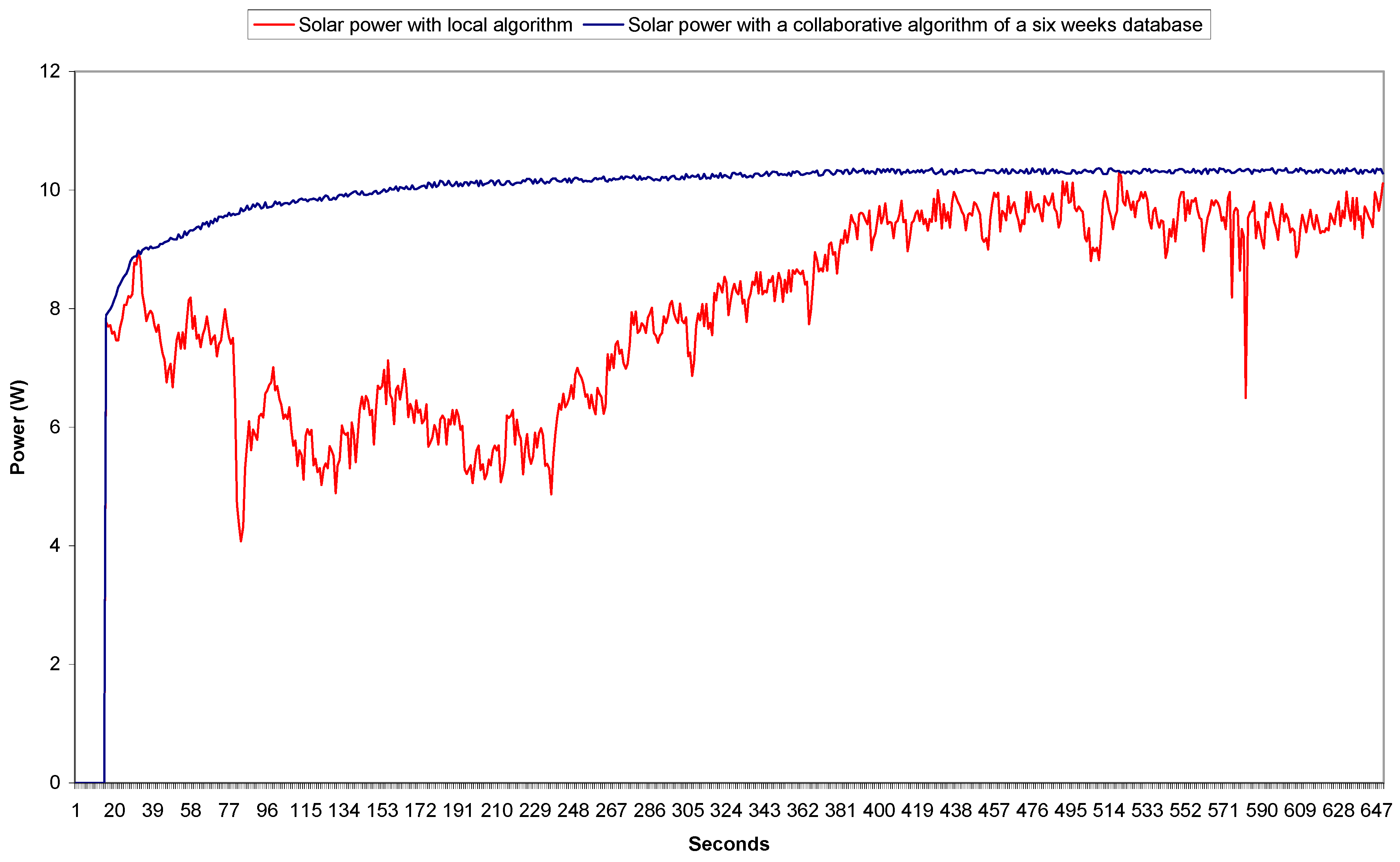
In order to show the influence of the flow of time and the impact of the latter as a positive factor on the behavior of our system at the SOC of the battery, the local algorithm is left to work as the only customer on the Firebase platform where the database is amplified locally only as a function of time. In the Figure 13, Figure 14, Figure 15, Figure 16 and Figure 17, the first plot obtained by the test given in Figure 11 is kept. It shows the evolution of the state of the battery by the local algorithm in order to draw on the same plan the system response after a few days to compare while keeping the same conditions and the previous initial state of the battery during three days, one week, two weeks, and one month, respectively.

We note here that the effect of the collaborative algorithm only according to the time is positive and this is due to the amplification of the database under Firebase locally, without the intervention of collaborators. It is noted from the run that there is an advance of 0.45% during a test interval of 10 min for the collaborative algorithm.

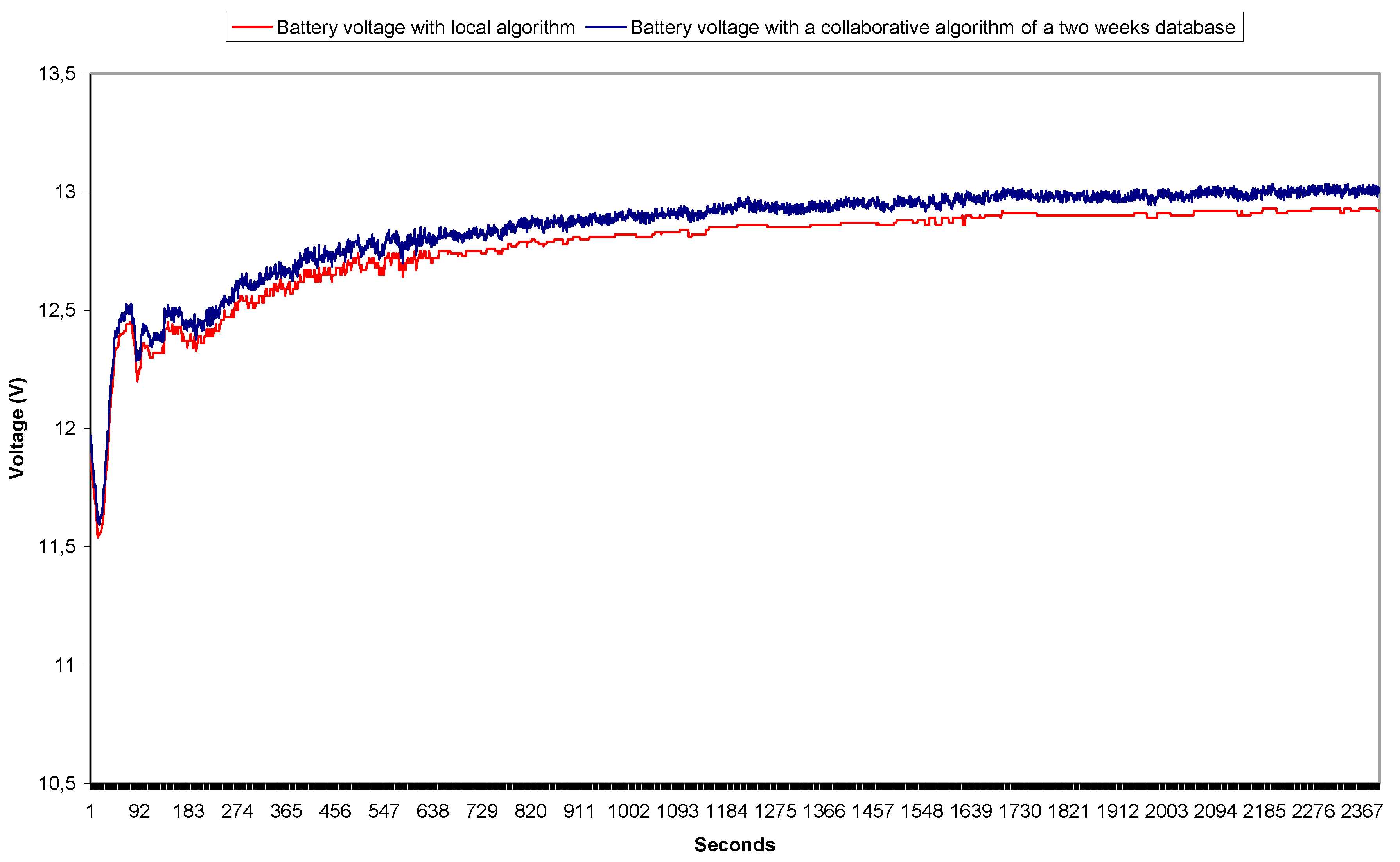
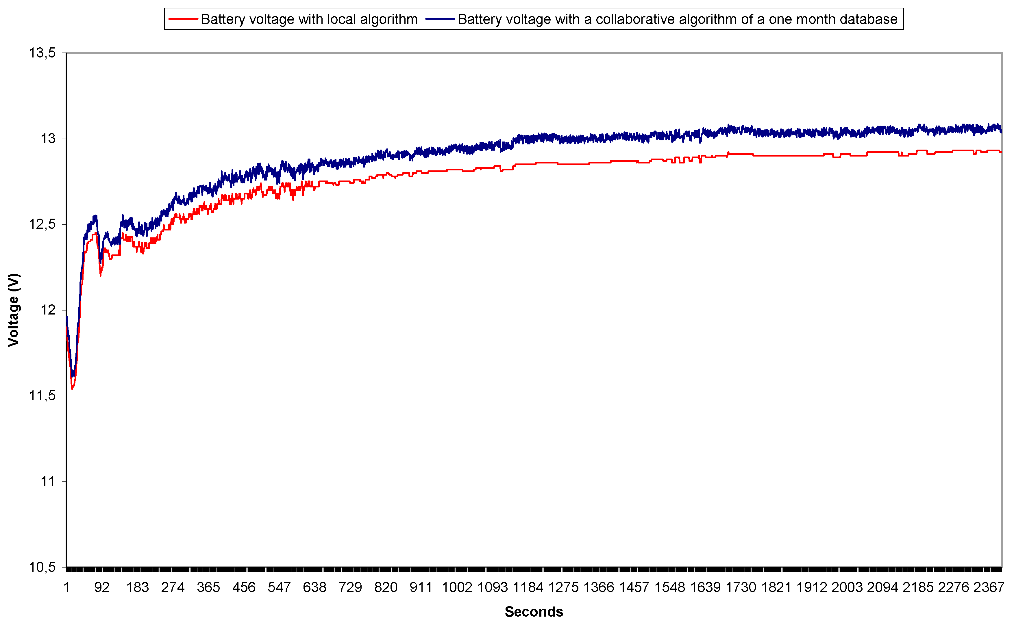
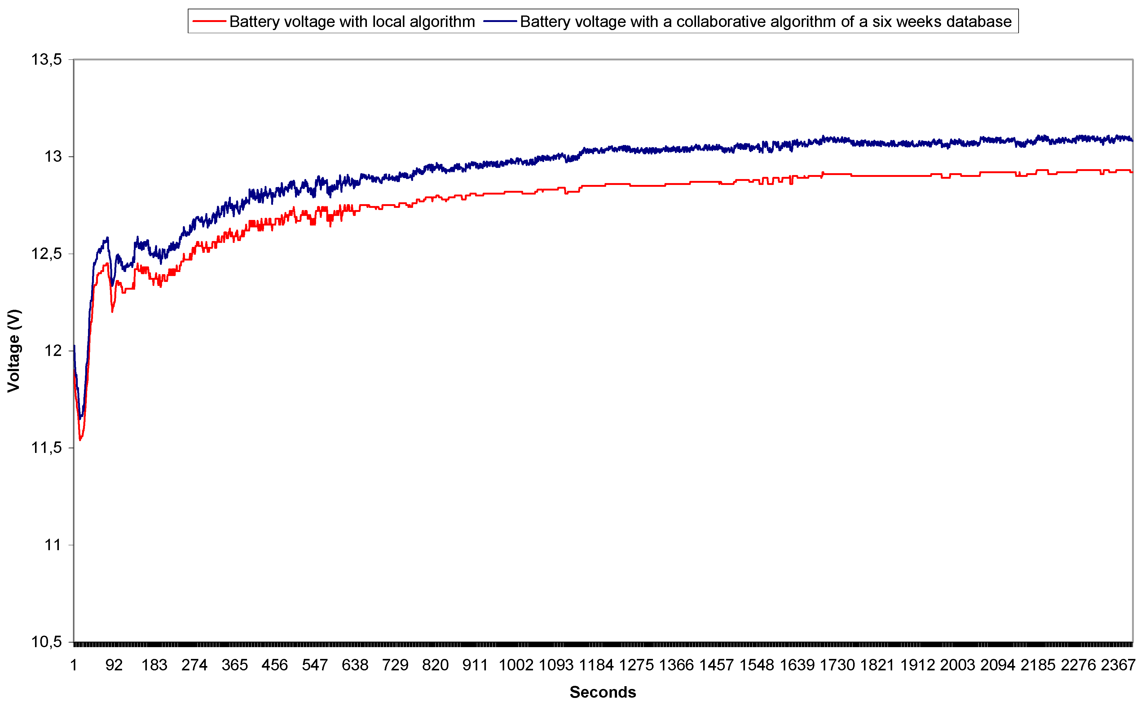
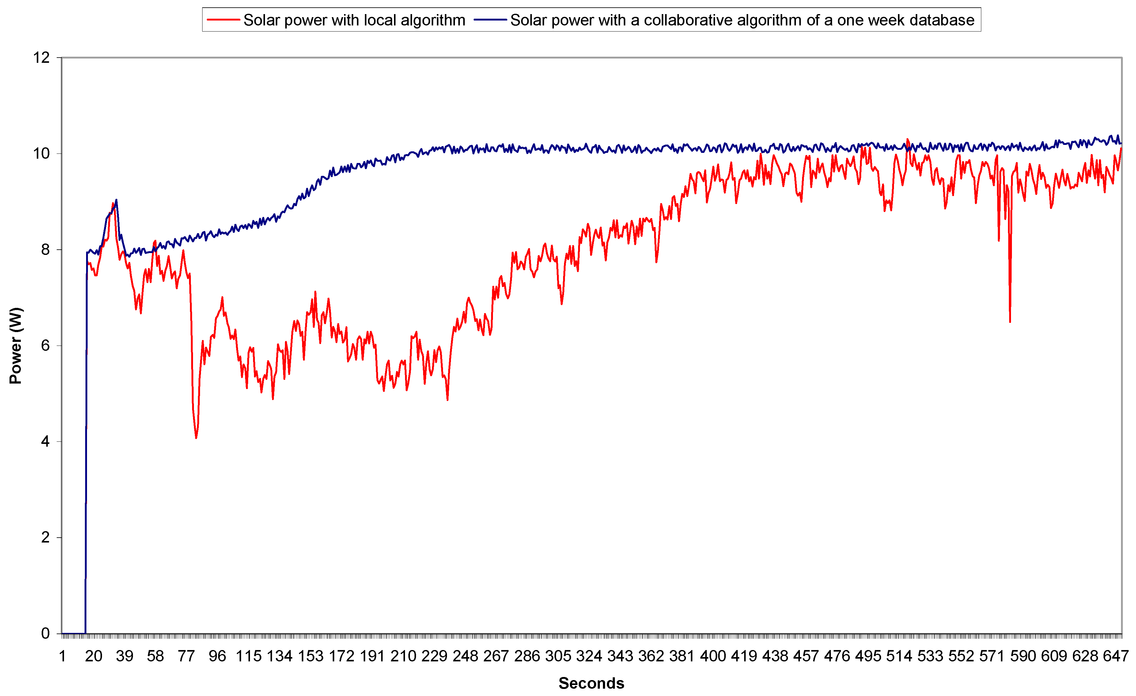
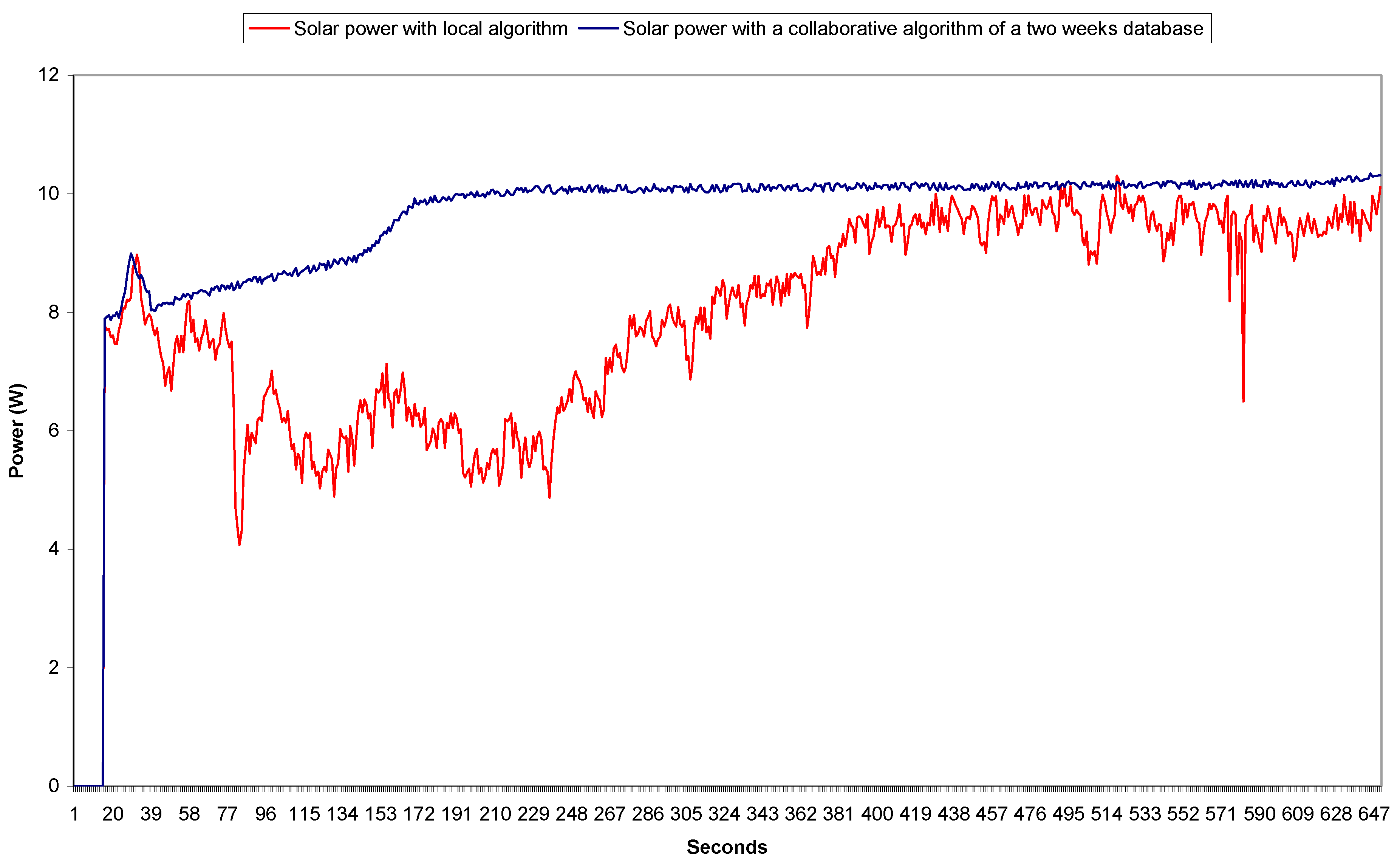
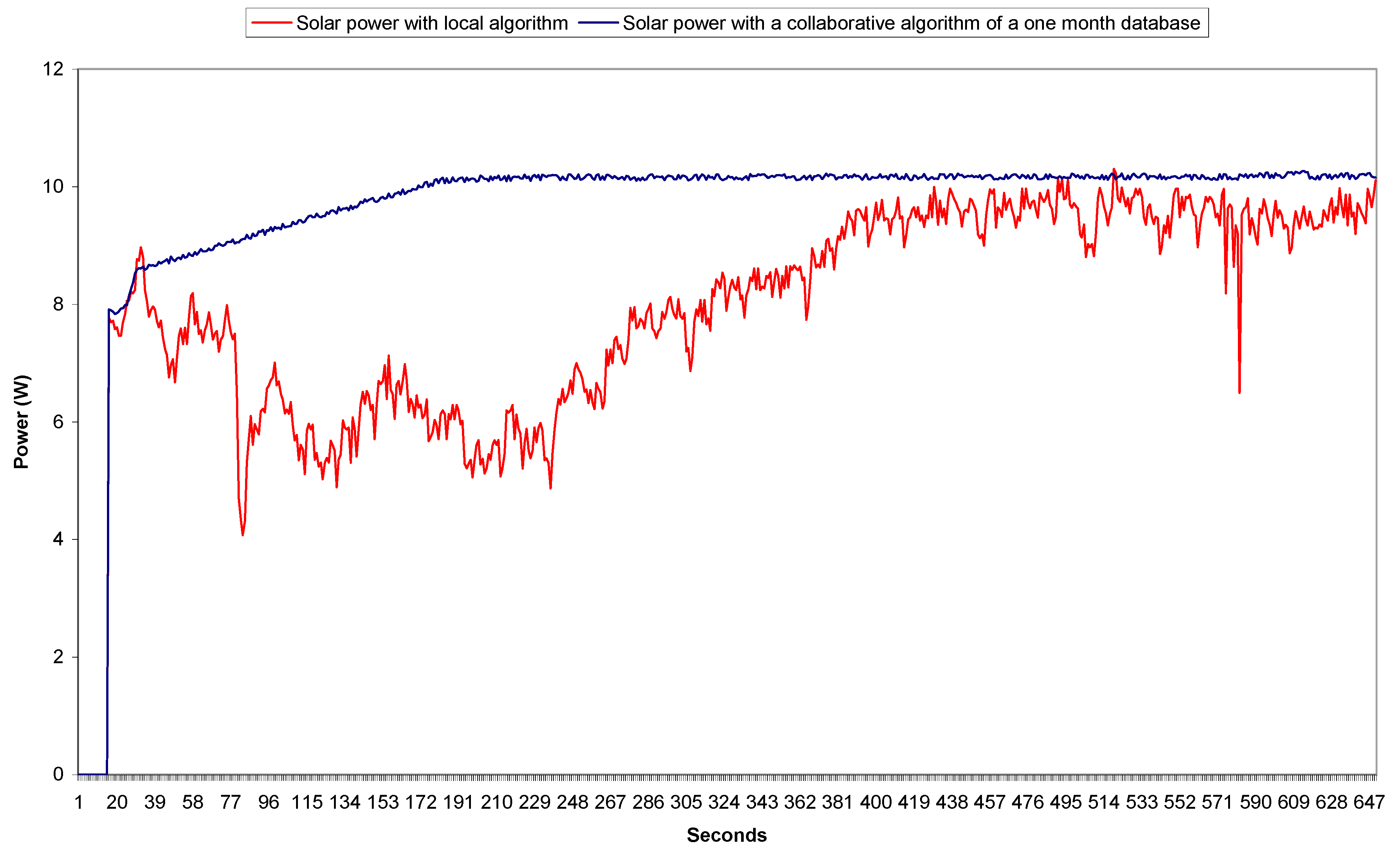
The same effect is found in Figure 14, Figure 15, Figure 16 and Figure 17 with a gain percentage that is higher at each extension of the database amplification time. These gains are respectively 0.51, 0.79, 0.91, and 0.98%. We deduce that the more we maintained our system linked by the application to Firebase the more we contributed to amplify the database. This allowed the system to learn to select the best duty cycle at the best time (it represents time corresponding to the selected duty cycle who is changed by the corresponding time) without loss of time and without calculations. This resulted in a faster loading rate and a more accurate probability of achieving MPP. Disturbances represent the time lost by the map to select the best duty cycle of the database.

Figure 18, Figure 19, Figure 20, Figure 21 and Figure 22 show the solar power without and with the collaborative algorithm for an amplifiable database of three days, one week, two weeks, one month, and six weeks.

These results show that:

• The bigger the database, the lower the transient
• The bigger the database, the faster the battery charges
• The bigger the database, the quicker the power solar reaches a steady state

8. Conclusions

Due to the MPPT optimization techniques and the control of the state of appropriate charges, the overall cost can be reduced in a photovoltaic chain after diminishing the need for mechanical and electronic components. Each technique has specific benefits. Imagine the optimization rate if we collaborate between them regarding the great similarity between the inputs and outputs of the systems.

This article explored a new collaborative approach using an Arduino board and a smartphone application. This approach is used to designate the initial duty cycle corresponding to the MPP from a Firebase database; a database configured from the irradiation and temperature values collected and analyzed by optimization algorithms of different collaborating customers or even by the local user which guarantees an optimal improvement of the panel performance and the performance of the DC/DC converter on this chain. It also provides an algorithm that could converge to the best duty cycle in case there is no customer. That is in order to avoid errors caused by sudden fluctuations and keep a good SOC. The purpose of the scenarios is to verify the behavior of the program when facing the daily variations of the climatic conditions; in particular the irradiation and the temperature and their effects on the current and the tension generated by the solar panel where the collaborative algorithm has demonstrated its superiority over the local algorithm.

This ensures a maximum energy transfer to the battery and a better exploitation of the PV source. The battery life would also be increased because the battery is constantly operating at a higher SOC. According to our research, we can also minimize the time needed for the algorithm to lead to the best SOC of the battery. In addition, the need for a powerful local algorithm is eliminated.