Data-Driven Approaches for Computation in Intelligent Biomedical Devices: A Case Study of EEG Monitoring for Chronic Seizure Detection


Abstract
:1. Introduction
2. The Need for Data-Driven Techniques
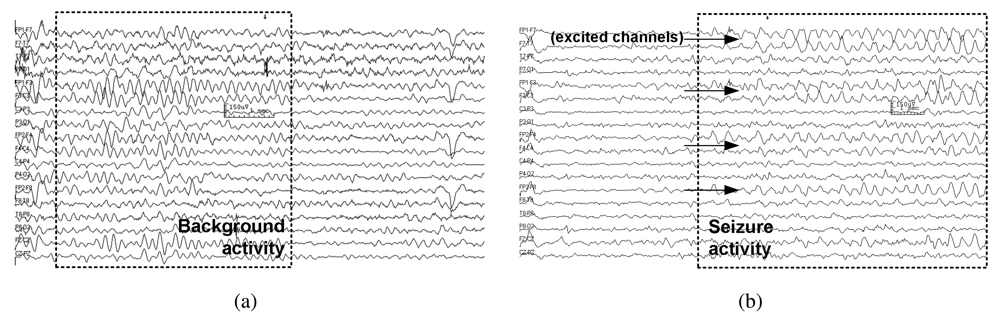
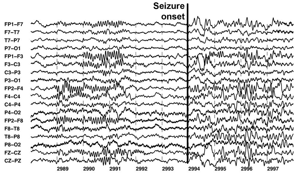
2.1. Detection Challenges in Biomedical Applications
2.2. Exploiting the Availability of Medical Data
3. Data-Driven Classification Frameworks
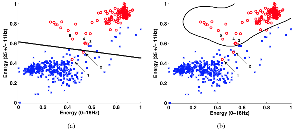
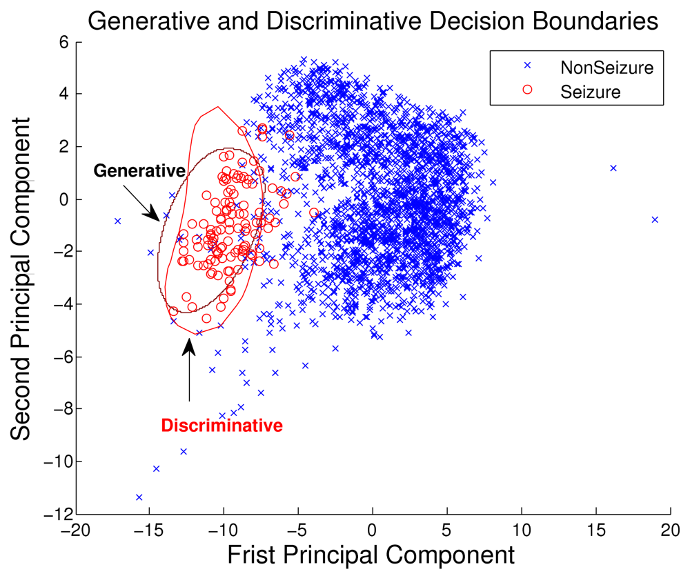
3.1. Discriminative Approach
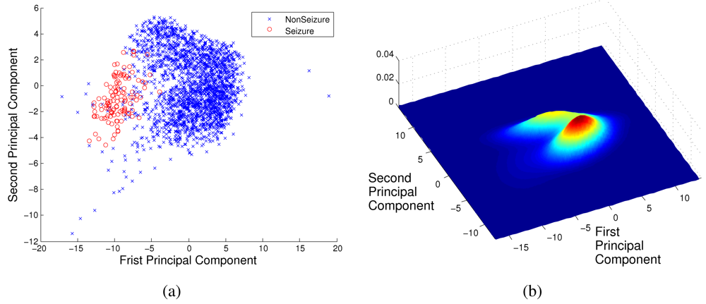
3.2. Generative Approach
4. Case Study: Chronic Seizure Detection System
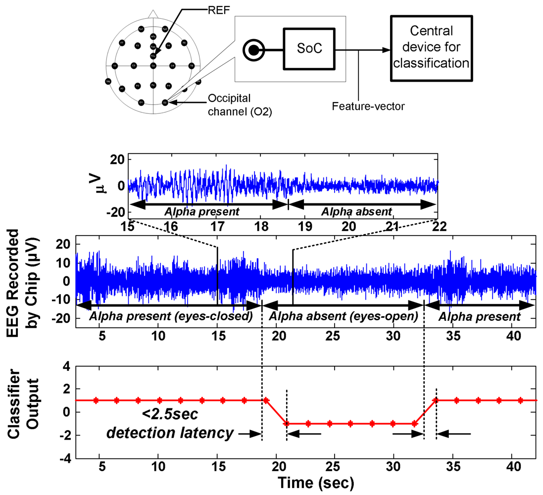
4.1. Algorithm and System Design
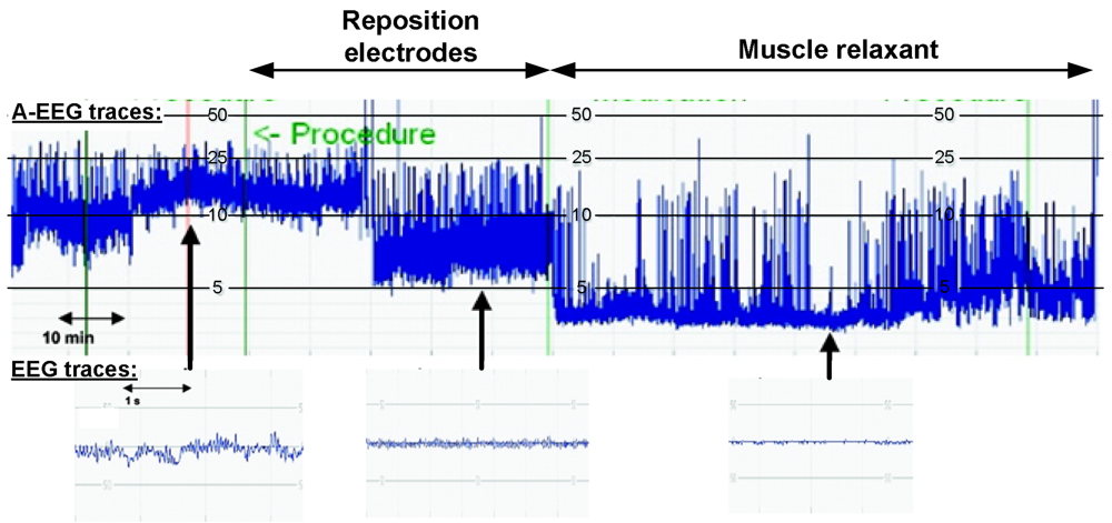
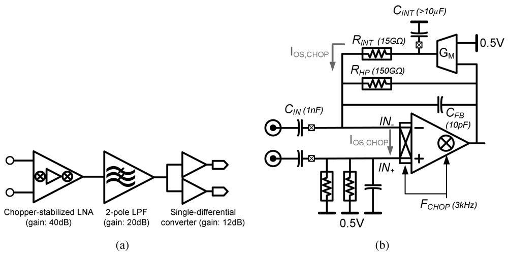
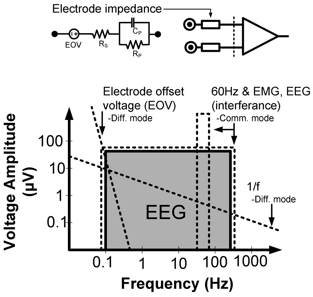
4.2. Low-Noise EEG Acquisition
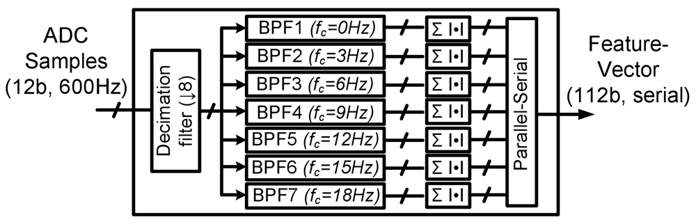
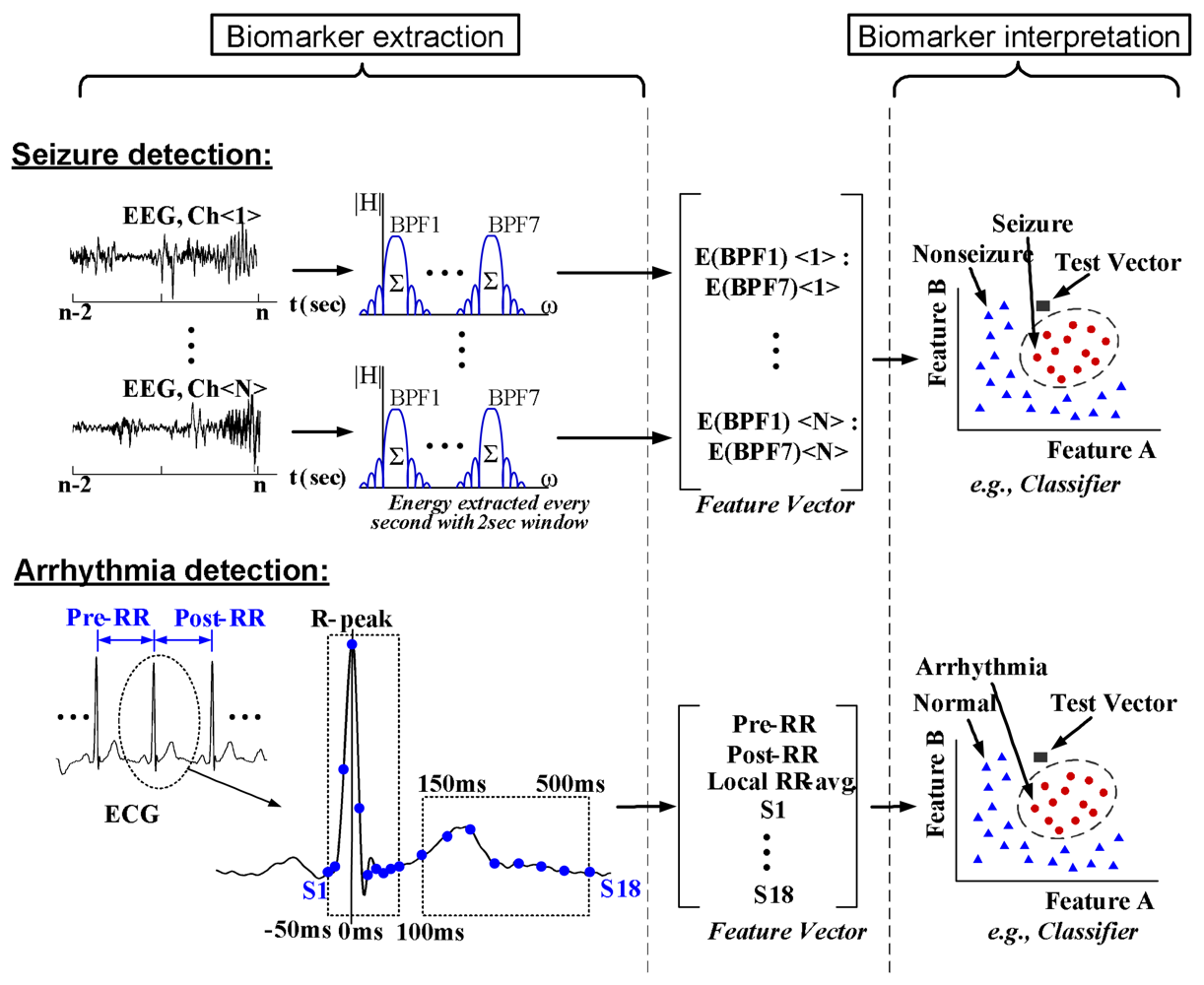
4.3. Feature-extraction Processing
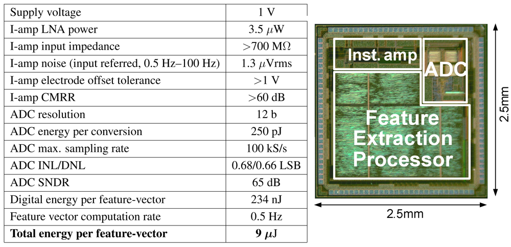
4.4. SoC Performance
4.5. Low-energy Programmable Processors Through Voltage Scaling
5. Conclusions and Challenges


| No Local Processing | Local Feature Extraction | |
|---|---|---|
| Instrumentation amps | 72 μW | 72 μW |
| ADCs (12 b, 600 Hz/ch.) | 3 μW | 3 μW |
| Digital Processors | - | 2.1 μW |
Radio (CC2550)
| 1733 μW
| 43 μW
|
| Total | 1808 μW | 120 μW |
| Feature Extraction Parameters | Parameter Values |
|---|---|
| Decimation filter input rate | 600 Hz |
| Decimation filter output rate | 75 Hz |
| Decimation filter BW | 150 Hz |
| Decimation filter input precision | 12-bits |
| Decimation filter output precision | 16-bits |
| Decimation filter order | 48 |
| Spectral analysis band | 0–20 Hz |
| Spectral analysis bins | 7 |
| Spectral analysis filter BW | 3 Hz |
| Spectral analysis filter pass band | 3 Hz |
| Spectral analysis filter output precision | 16-bits |
| Spectral analysis filter order | 46 |
Acknowledgments
References and Notes
- Benabid, A.L. Deep brain stimulation for Parkinson's disease. Curr. Opin. Neurobiol. 2003, 13, 696–706. [Google Scholar]
- Schachter, S.C. Vagus nerve stimulator. Epilepsia 1998, 39, 677–686. [Google Scholar]
- Kim, D.H.; Viventi, J.; Amsden, J.; Xiao, J.; Vigeland, L.; Kim, Y.S.; Blanco, J.; Frechette, E.; Contreras, D.; Kaplan, D.; et al. Dissolvable films of silk fibroin for ultrathin, conformal bio-integrated electronics. Nat. Mater. 2010, 9, 511–517. [Google Scholar]
- Graudejus, O.; Yu, Z.; Jones, J.; Morrison, B.; Wagner, S. Characterization of an elastically stretchable microelectrode array and its application to neural field potential recordings. J. Electrochem. Soc. 2009, 156, 85–94. [Google Scholar]
- Viventi, J.; Kim, D.H.; Moss, J.; Kim, Y.S.; Blanco, J.; Anetta, N.; Hicks, A.; Xiao, J.; Huang, Y.; Callans, D.J.; et al. Dissolvable films of silk fibroin for ultrathin, conformal bio-integrated electronics. Sci. Trans. Med. 2010, 2, 2694–2699. [Google Scholar]
- Chandrakasan, A.; Verma, N.; Daly, D. Ultralow-power electronics for biomedical applications. Annu. Rev. Biomed. Eng. 2008, 10, 247–274. [Google Scholar]
- Leong, T.; Aronsky, D.; Michael Shabot, M. Guest editorial: Computer-based decision support for critical and emergency care. J. Biomed. Inform. 2008, 41, 409–412. [Google Scholar]
- Wallis, L. Alarm fatigue linked to patient's death. Am. J. Nurs. 2010, 110, 16. [Google Scholar]
- Dishman, E. Inventing wellness systems for aging in place. IEEE Comput. 2004, 37, 34–41. [Google Scholar]
- Tsien, C. TrendFinder: Automated detection of alarmable trends. Ph.D. Thesis, Massachusetts Institute of Technology, Cambridge, MA, USA, 2000. [Google Scholar]
- Tompkins, W.J. Biomedical Digital Signal Processing: C Language Examples and Laboratory Experiments for the IBM PC; Prentice-Hall: Bergen County, NJ, USA, 1993. [Google Scholar]
- Hau, D.; Coiera, E. Learning Qualitative Models from Physiological Signals AAAI Technical Report SS-94-01. 1994, 67–71.
- Hagmann, C.F.; Robertson, N.J.; Azzopardi, D. Artifacts on electroencephalograms may influence the amplitude-integrated EEG classification: A qualitative analysis in neonatal encephalopathy. Pediatrics 2006, 118, 2552–2554. [Google Scholar]
- Yazicioglu, R. Biopotential Readout Circuits for Portable Acquisition Systems. Ph.D. Thesis, Katholieke Universiteit, Leuven, Belgium, 2008. [Google Scholar]
- Shoeb, A.; Schachter, S.; Schomer, D.; Bourgeois, B.; Treves, S.T.; Guttag, J. Detecting seizure onset in the ambulatory setting: Demonstrating feasibility. Conf. Proc. IEEE Eng. Med. Biol. Soc. 2005, 4, 3546–3550. [Google Scholar]
- Gotman, J.; Ives, J.; Gloor, G. Frequency content of eeg and emg at seizure onset: Possibility of removal of EMG artefact by digital filtering. EEG Clin. Neurophysiol. 1981, 52, 626–639. [Google Scholar]
- Shoeb, A.; Bourgeois, B.; Treves, S.; Schachter, S.; Guttag, J. Impact of patient-specificity on seizure onset detection performance. Proceedings of the International Conference of the IEEE Engineering in Medicine and Biology Society, Lyon, France, 2007; pp. 4110–4114.
- Meyfroidt, G.; Guiza, F.; Ramon, J.; Bruynooghe, M. Machine learning techniques to examine large patient databases. Best Pract. Res. Clin. Anaesthesiol. 2009, 23, 127–143. [Google Scholar] [Green Version]
- Sajda, P. Machine learning for diagnosis and detection of disease. Annu. Rev. Biomed. Eng. 2006, 8, 537–565. [Google Scholar]
- Podgorelec, V.; Druzovec, T.W. Some applications of intelligent systems in medicine. Proceedings of the IEEE 3rd International Conference on Computational Cybernetics, Mauritius, 2005; pp. 35–39.
- Shoeb, A.; Guttag, J. Application of Machine Learning to Epileptic Seizure Detection. Proceedings of the International Conference on Machine Learning, Haifa, Israel, 2010.
- de Chazal, P.; O'Dwyer, M.; Reilly, R.B. Automatic classification of heartbeats using ECG morphology and heartbeat interval features. IEEE Trans. Biomed. Eng. 2004, 51, 1196–1206. [Google Scholar]
- Sorenson, D.; Grissom, C.; Carpenter, L.; Austin, A.; Sward, K.; Napoli, L.; Warner, H.; Morris, A. and for the Reengineering Clinical Research in Critical Care Investigators. A frame-based representation for a bedside ventilator weaning protocol. J. Biomed. Inform. 2008, 41, 461–468. [Google Scholar]
- Jouny, C.; Bergey, G. Dynamics of Epileptic Seizures During Evolution And Propagation. In Computational Neuroscience in Epilepsy, 1st ed.; Soltesz, I., Staley, K., Eds.; Academic Press: San Diego, CA, USA, 2008; Volume 28, pp. 457–470. [Google Scholar]
- Hsu, C.W.; Lin, C.J. A comparison of methods for multiclass support vector machines. IEEE Trans. Neural Networks 2002, 13, 415–425. [Google Scholar]
- Rubinstein, Y.D.; Hastie, T. Discriminative vs Informative Learning. Proceedings of the 3rd International Conference on Knowledge Discovery and Data Mining; AAAI Press: Menlo Park, CA, USA, 1997; pp. 49–53. [Google Scholar]
- Ng, A.Y.; Jordan, M.I. On Discriminative vs. Generative classifiers: A comparison of logistic regression and naive Bayes. Adv. Neural Inf. Process. Syst. 2001, 14, 841–848. [Google Scholar]
- Cristianini, N.; Shawe-Taylor, J. An Introduction to Support Vector Machines and Other Kernel Based Learning Methods; Cambridge University Press: Cambridge, UK, 2000. [Google Scholar]
- If the classes cannot be well separated by a hyper-plane, the SVM can be used to determine a quadratic or circumferential decision boundary. The SVM determines a nonlinear boundary in the input feature space by solving for linear boundary in higher-dimensional feature space, which is formed by introducing a kernel.
- Theodoridis, S.; Koutroumbas, K. Linear Classifiers. In Pattern Recognition; Elsevier: Oxford, UK, 2009; Chapter 3. [Google Scholar]
- Joachims, T. Text Categorization with Support-Vector Machines: Learning with Many Relevant Features. Proceedings of the European Conference on Machine Learning; Springer: Berlin, Germany, 1998; pp. 137–142. [Google Scholar]
- Akbani, R.; Kwek, S.; Japkowicz, N. Applying Support-Vector Machines to Imbalanced Datasets. Proceedings of the European Conference on Machine Learning; Springer: Berlin, Germany, 2004. [Google Scholar]
- Kay, S.M. Cramer-Rao Lower Bound. In Fundamentals of Statistical Signal Processing: Detection Theory; Prentice-Hall: Bergen County, NJ, USA, 1998; Chapter 3; pp. 60–92. [Google Scholar]
- Bishop, C.M. Probability Distributions. In Pattern Recognition and Machine Learning; Springer: Berlin, Germany, 2006; Chapter 2; pp. 67–127. [Google Scholar]
- Lotte, F.; Congedo, M.; Lauyer, A.; Lamarche, F.; Arnaldi, B. A Review of Classification Algorithms for EEG-Based Brain-Computer Interface. J. Neural Eng. 2007, 4, R1–R13. [Google Scholar]
- Shih, E.I. Reducing the Computational Demands of Medical Monitoring Classifiers by Examining Less Data. Ph.D. Thesis, Massachu-setts Institute of Technology, Cambridge, MA, USA, 2010. [Google Scholar]
- Avestruz, A.T.; Santa, W.; Carlson, D.; Jensen, R.; Stanslaski, S.; Helfenstine, A.; Denison, T. A 5 μW/channel spectral analysis IC for chronic bidirectional brain-machine interfaces. IEEE J. Solid-State Circuits 2008, 43, 3006–3024. [Google Scholar]
- Yazicioglu, R.F.; Kim, S.; Torfs, T.; Merken, P.; Hoof, C.V. A 30 μW analog signal processor ASIC for biomedical signal monitoring. Proceedings of the IEEE International Solid-State Circuits Conference Digest of Technical Papers (ISSCC), San Francisco, CA, USA, 2010; pp. 124–125.
- Shoeb, A.; Carlson, D.; Panken, E.; Denison, T. A Micropower Support Vector Machine Based Seizure Detection Architecture for Embedded Medical Devices. Proceedings of the Annual International Conference of the IEEE Engineering in Medicine and Biology Society (EMBC 2009), Minneapolis, MN, USA, 2009; pp. 4202–4205.
- Texas Instruments. Low-cost low-power 2.4 GHz RF transmitter. Available Online: http://focus.ti.com/docs/prod/folders/print/cc2550.html (accessed on 1 September 2010).
- Verma, N.; Shoeb, A.; Bohorquez, J.; Dawson, J.; Guttag, J.; Chandrakasan, A.P. A micro-power EEG acquisition SoC with integrated feature extraction processor for a chronic seizure detection system. IEEE J. Solid-State Circuits 2010, 45, 804–816. [Google Scholar]
- Dozio, R.; Baba, A.; Assambo, C.; Burke, M.J. Time based measurement of the impedance of the skin-electrode interface for dry electrode ECG recording. Proceedings of the 29th Annual International Conference of the IEEE Engineering in Medicine and Biology Society (EMBC 2007), Lyon, France, 2007; pp. 5001–5004.
- Enz, C.; Temes, G. Circuit techniques for reducing the effects of op-amp imperfections: auto-zeroing, correlated double sampling, and chopper stabilization. Proc. IEEE 1996, 84, 1584–1614. [Google Scholar]
- Denison, T.; Consoer, K.; Santa, W.; Avestruz, A.T.; Cooley, J.; Kelly, A. A 2 μW 100 nV/rtHz chopper-stabilized instrumentation amplifier for chronic measurement of neural field potentials. IEEE J. Solid-State Circuits 2007, 42, 2934–2945. [Google Scholar]
- Yazicioglu, R.; Merken, P.; Puers, R.; Hoof, C.V. A 60 μW 60 readout front-end for portable biopotential acquisition system. IEEE J. Solid-State Circuits 2007, 42, 1100–1110. [Google Scholar]
- Verma, N.; Chandrakasan, A.P. An ultra low energy 12-bit rate-resolution scalable SAR ADC for wireless sensor nodes. IEEE J. Solid-State Circuits 2007, 42, 1196–1205. [Google Scholar]
- Wang, A.; Chandrakasan, A.P. A 180 mV subthreshold FFT processor using a minimum energy design methodology. IEEE J. Solid-State Circuits 2005, 40, 310–319. [Google Scholar]
- Kwong, J.; Ramadass, Y.K.; Verma, N.; Chandrakasan, A. A 65 nm Sub-Vt microcontroller with integrated SRAM and switched capacitor DC-DC converter. IEEE J. Solid-State Circuits 2009, 44, 115–126. [Google Scholar]
- Verma, N. Ultra-Low-Power SRAM Design In High Variability Advanced CMOS. Ph.D. Thesis, Massachusetts Institute of Technology, Cambridge, MA, USA, 2009. [Google Scholar]
- Kwong, J.; Chandrakasan, A. Variation-Driven Device Sizing for Minimum Energy Sub-threshold Circuits. Proceedings of the International Symposium on Low Power Electronics and Design, Tegernsee, Germany, 2006; pp. 8–13.
©2011 by the authors; licensee MDPI, Basel, Switzerland. This article is an open access article distributed under the terms and conditions of the Creative Commons Attribution license (http://creativecommons.org/licenses/by/3.0/).
Share and Cite
Verma, N.; Lee, K.H.; Shoeb, A. Data-Driven Approaches for Computation in Intelligent Biomedical Devices: A Case Study of EEG Monitoring for Chronic Seizure Detection. J. Low Power Electron. Appl. 2011, 1, 150-174. https://doi.org/10.3390/jlpea1010150
Verma N, Lee KH, Shoeb A. Data-Driven Approaches for Computation in Intelligent Biomedical Devices: A Case Study of EEG Monitoring for Chronic Seizure Detection. Journal of Low Power Electronics and Applications. 2011; 1(1):150-174. https://doi.org/10.3390/jlpea1010150
Chicago/Turabian StyleVerma, Naveen, Kyong Ho Lee, and Ali Shoeb. 2011. "Data-Driven Approaches for Computation in Intelligent Biomedical Devices: A Case Study of EEG Monitoring for Chronic Seizure Detection" Journal of Low Power Electronics and Applications 1, no. 1: 150-174. https://doi.org/10.3390/jlpea1010150