
The Impact of Photobleaching on Microarray Analysis


Abstract
:
1. Introduction
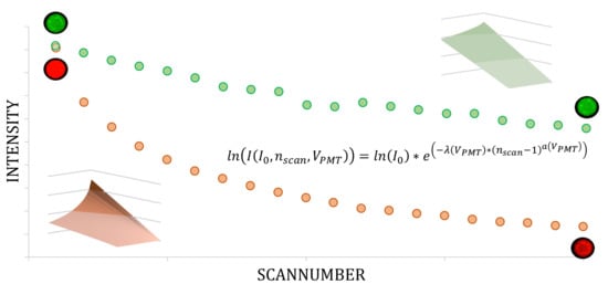
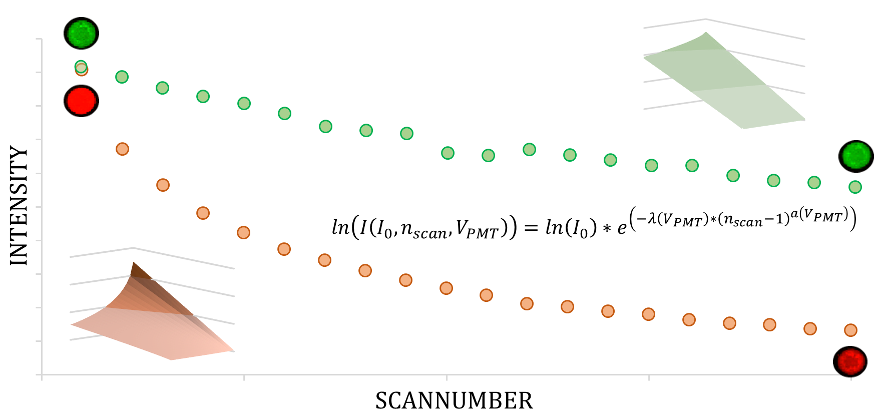
2. Model
3. Experimental Section
3.1. Oligo Preparation
3.2. DNA Immobilization
3.3. Data Acquisition

| # Chip | PMT635 nm [V] | PMT532 nm [V] |
|---|---|---|
| 1 | 950 | 700 |
| 2 | 850 | 600 |
| 3 | 750 | 500 |
| 4 | 650 | 400 |
| 5 | 550 | 300 |
| # Scan | PMT635 nm [V] | PMT532 nm [V] |
|---|---|---|
| 1 | 550 | 300 |
| 2 | 650 | 400 |
| 3 | 750 | 500 |
| 4 | 850 | 600 |
| 5 | 950 | 700 |
3.4. Data Analysis
3.4.1. Post Processing
3.4.2. Modeling
3.4.3. Validation
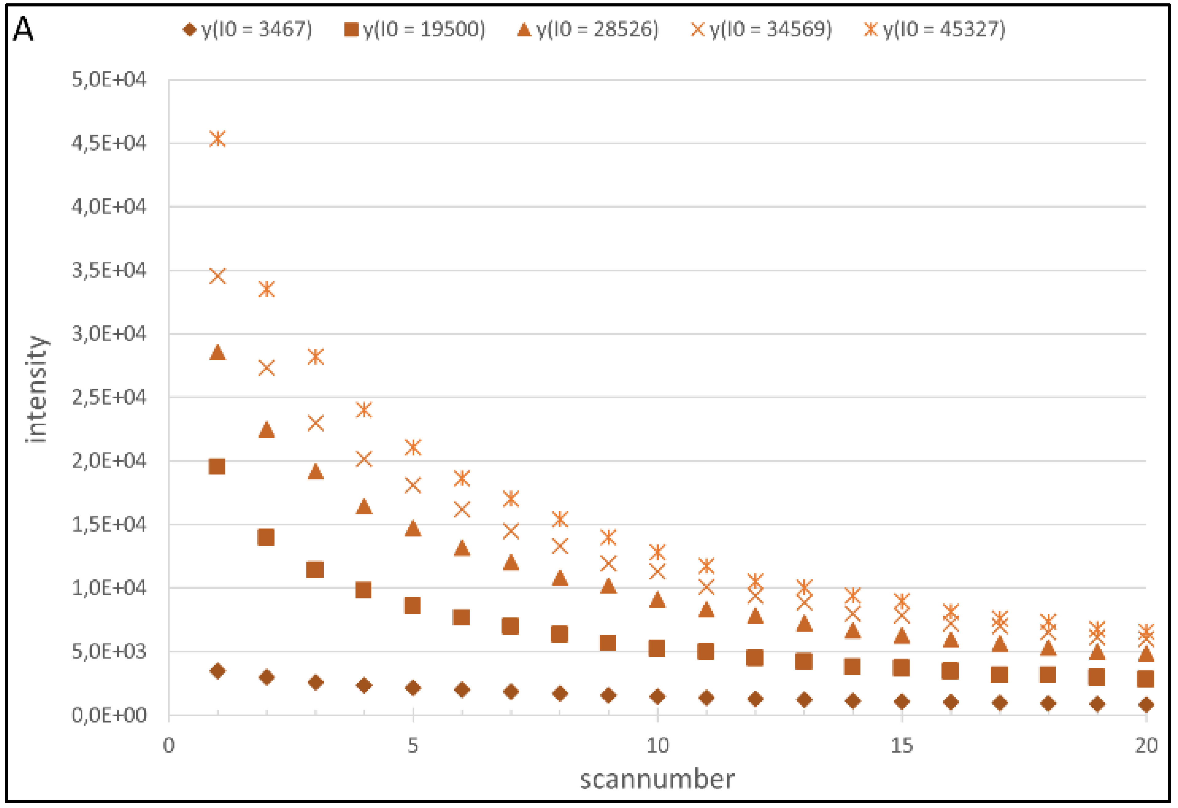
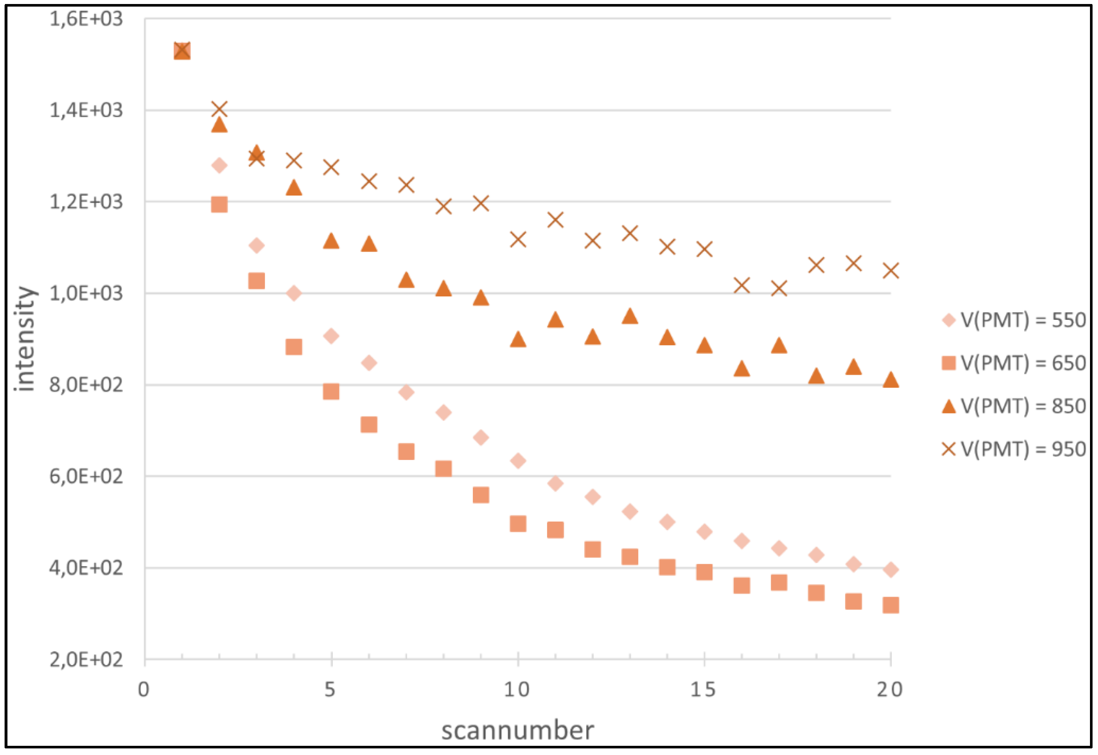
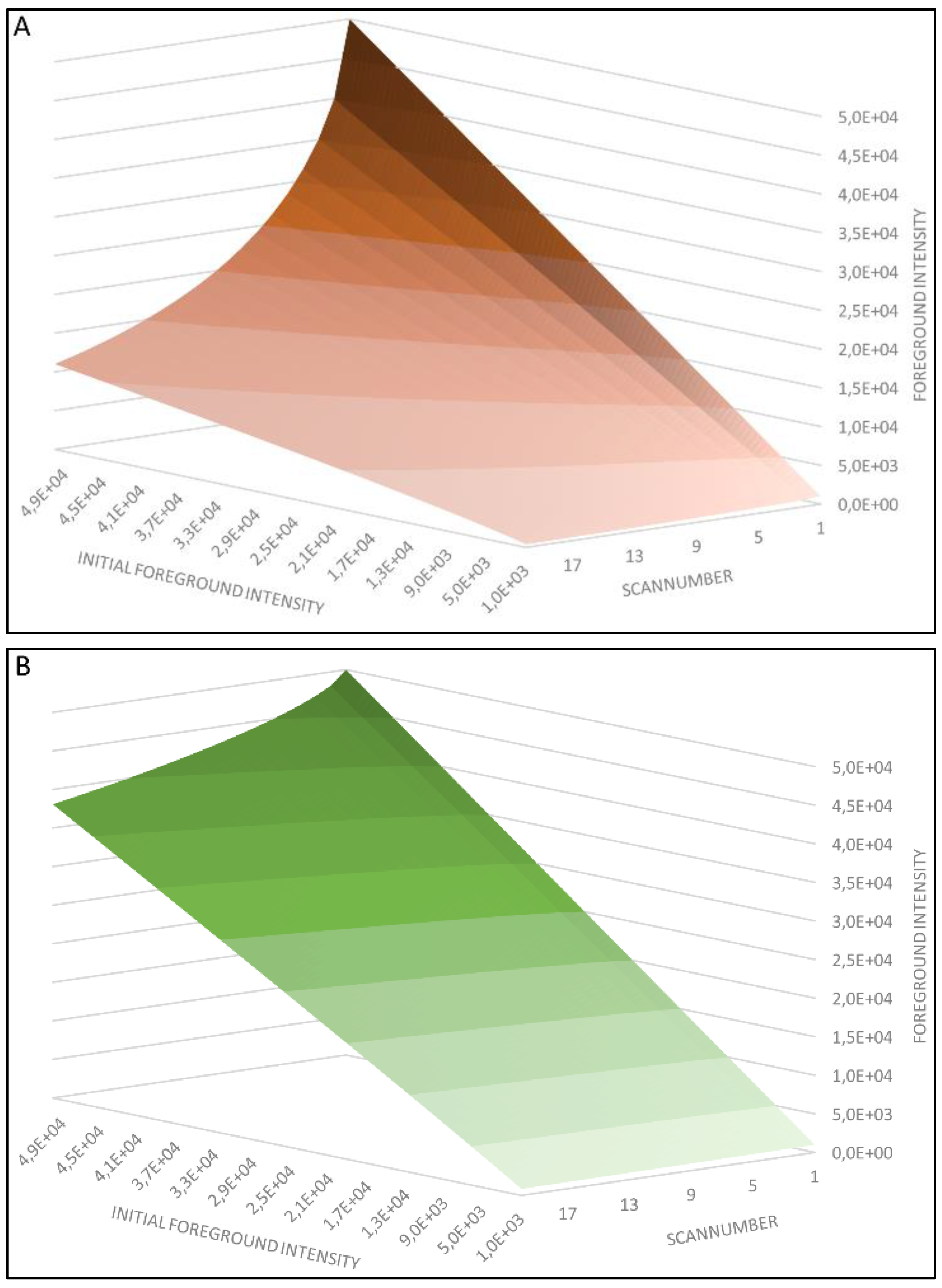
4. Results and Discussion
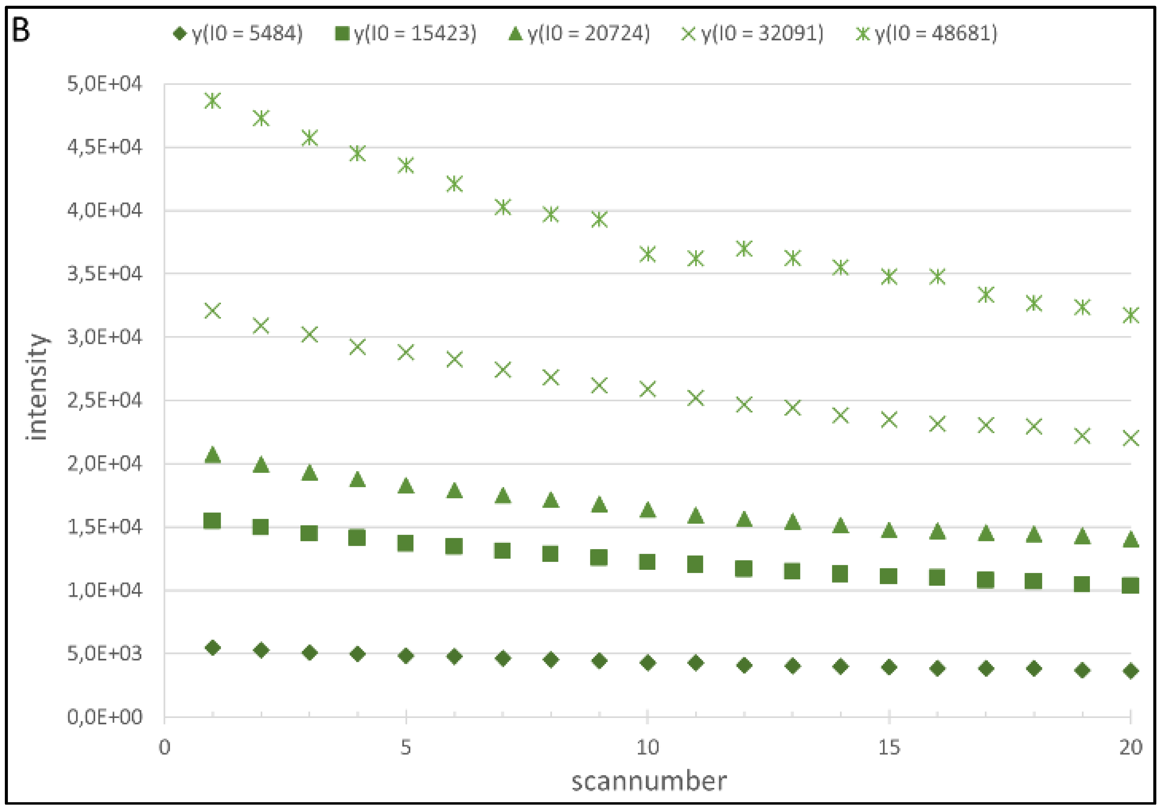
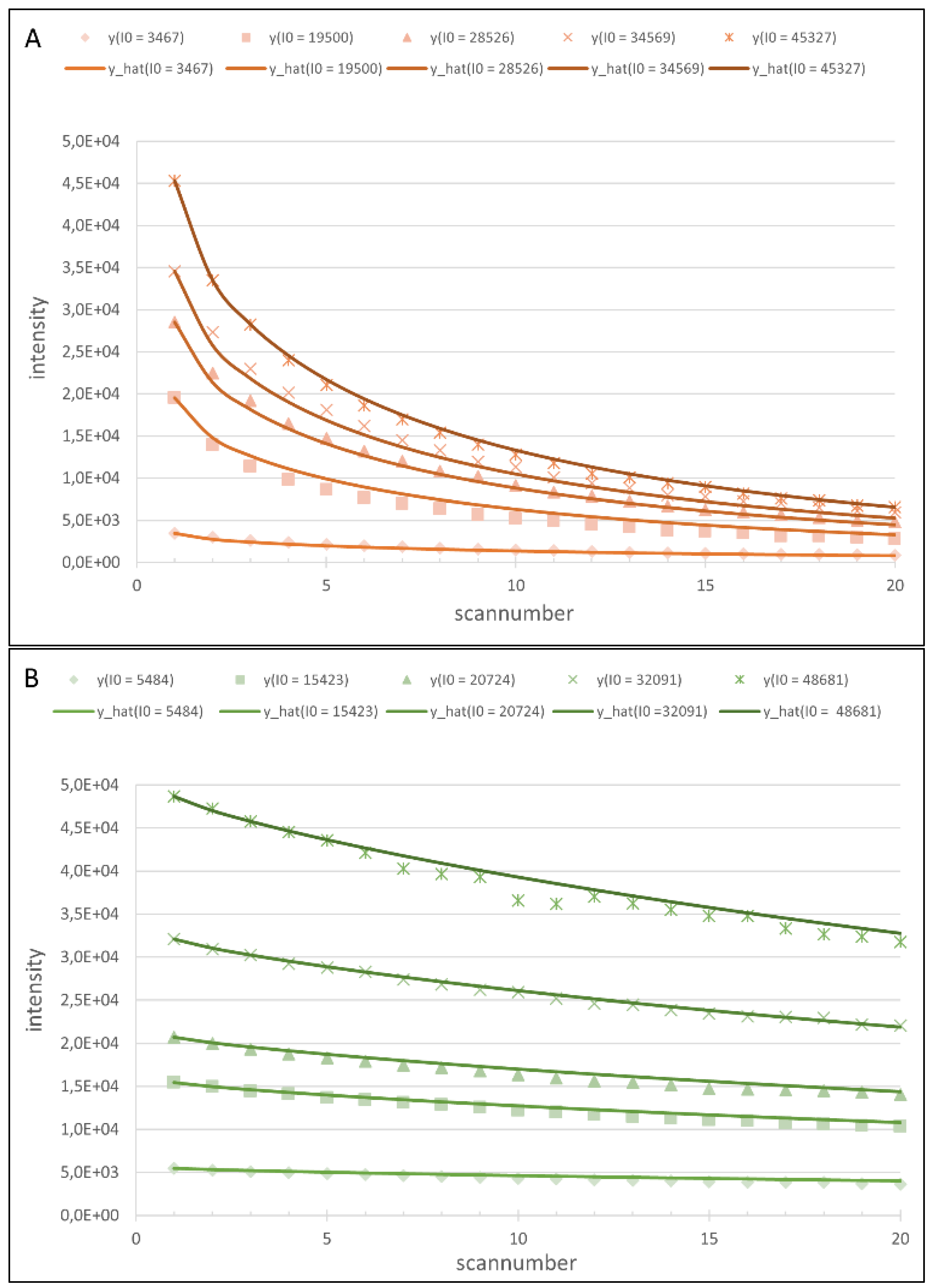
4.1. Regression Analysis

4.2. Generation of the Cy5 and Cy3 Model
| Fluorophore | λ (VPMT) | a(VPMT) | ||||
|---|---|---|---|---|---|---|
| p1 | p2 | p3 | p1 | p2 | p3 | |
| Cy3 | −2.153E−07 | 3.232E−04 | −9.200E−02 | 1,106E−06 | −1.885E−03 | 1.461 |
| Cy5 | −1.122E−08 | 1.640E−5 | −1.948E−03 | −4.533E−07 | 9.433E−05 | 0.901 |
4.3. Model Analysis
4.4. First Model Validation

| Fluorophore | Regression Feature | Data Source | |
|---|---|---|---|
| Raw Validation Data | Model Corrected Validation Data | ||
| Cy5 | |||
| Cy3 | |||
5. Conclusions
Supplementary Files
Supplementary File 1Author Contributions
Conflicts of Interest
References
- Spielbauer, B.; Stahl, F. Impact of microarray technology in nutrition and food research. Mol. Nutr. Food Res. 2005, 49, 908–917. [Google Scholar] [CrossRef] [PubMed]
- Allison, D.B.; Cui, X.; Page, G.P.; Sabripour, M. Microarray data analysis: From disarray to consolidation and consensus. Nat. Rev. Genet. 2006, 7, 55–65. [Google Scholar] [CrossRef] [PubMed]
- Ehrenreich, A. DNA microarray technology for the microbiologist: An overview. Appl. Microbiol. Biotechnol. 2006, 73, 255–273. [Google Scholar] [CrossRef] [PubMed]
- Kretschy, N.; Somoza, M.M. Comparison of the sequence-dependent fluorescence of the cyanine dyes cy3, cy5, dylight dy547 and dylight dy647 on single-stranded DNA. PLoS ONE 2014, 9, e85605. [Google Scholar] [CrossRef] [PubMed]
- Mary-Huard, T.; Daudin, J.J.; Robin, S.; Bitton, F.; Cabannes, E.; Hilson, P. Spotting effect in microarray experiments. BMC Bioinf. 2004. [Google Scholar] [CrossRef] [PubMed] [Green Version]
- Dawson, E.D.; Reppert, A.E.; Rowlen, K.L.; Kuck, L.R. Spotting optimization for oligo microarrays on aldehyde-glass. Anal. Biochem. 2005, 341, 352–360. [Google Scholar] [CrossRef] [PubMed]
- Sobek, J.; Aquino, C.; Weigel, W.; Schlapbach, R. Drop drying on surfaces determines chemical reactivity-the specific case of immobilization of oligonucleotides on microarrays. BMC Biophys. 2013. [Google Scholar] [CrossRef] [PubMed]
- Rao, A.N.; Grainger, D.W. Biophysical properties of nucleic acids at surfaces relevant to microarray performance. Biomater. Sci. 2014, 2, 436–471. [Google Scholar] [CrossRef] [PubMed]
- Jang, H.; Cho, M.; Kim, H.; Kim, C.; Park, H. Quality control probes for spot-uniformity and quantitative analysis of oligonucleotide array. J. Microbiol. Biotechnol. 2009, 19, 658–665. [Google Scholar] [PubMed]
- Khondoker, M.R.; Glasbey, C.A.; Worton, B.J. Statistical estimation of gene expression using multiple laser scans of microarrays. Bioinformatics 2006, 22, 215–219. [Google Scholar] [CrossRef] [PubMed]
- Satterfield, M.B.; Lippa, K.; Lu, Z.Q.; Salit, M.L. Microarray scanner performance over a five-week period as measured with cy5 and cy3 serial dilution slides. J. Res. Natl. Inst. Stand. Technol. 2008, 113, 157–174. [Google Scholar] [CrossRef]
- Ambroise, J.; Bearzatto, B.; Robert, A.; Macq, B.; Gala, J.L. Combining multiple laser scans of spotted microarrays by means of a two-way anova model. Statist. Appl. Genet. Mol. Biol. 2012. [Google Scholar] [CrossRef] [PubMed]
- Vora, G.J.; Meador, C.E.; Anderson, G.P.; Taitt, C.R. Comparison of detection and signal amplification methods for DNA microarrays. Mol. Cell. Probes 2008, 22, 294–300. [Google Scholar] [CrossRef] [PubMed]
- Shi, L.; Tong, W.; Su, Z.; Han, T.; Han, J.; Puri, R.K.; Fang, H.; Frueh, F.W.; Goodsaid, F.M.; Guo, L.; et al. Microarray scanner calibration curves: Characteristics and implications. BMC Bioinf. 2005. [Google Scholar] [CrossRef] [PubMed]
- Lyng, H.; Badiee, A.; Svendsrud, D.H.; Hovig, E.; Myklebost, O.; Stokke, T. Profound influence of microarray scanner characteristics on gene expression ratios: Analysis and procedure for correction. BMC Genomics 2004. [Google Scholar] [CrossRef] [Green Version]
- Dar, M.; Giesler, T.; Richardson, R.; Cai, C.; Cooper, M.; Lavasani, S.; Kille, P.; Voet, T.; Vermeesch, J. Development of a novel ozone- and photo-stable hyper5 red fluorescent dye for array cgh and microarray gene expression analysis with consistent performance irrespective of environmental conditions. BMC Biotechnol. 2008. [Google Scholar] [CrossRef] [PubMed]
- Kuang, C.; Luo, D.; Liu, X.; Wang, G. Study on factors enhancing photobleaching effect of fluorescent dye. Measurement 2013, 46, 1393–1398. [Google Scholar] [CrossRef]
- Drăghici, S. Statistics and Data Analysis for Microarrays Using r and Bioconductor, 2nd ed.; Taylor & Francis: Boca Raton, FL, USA, 2011. [Google Scholar]
- Dobbin, K.; Shih, J.H.; Simon, R. Statistical design of reverse dye microarrays. Bioinformatics 2003, 19, 803–810. [Google Scholar] [CrossRef] [PubMed]
- Gupta, R.; Auvinen, P.; Thomas, A.; Arjas, E. Bayesian hierarchical model for correcting signal saturation in microarrays using pixel intensities. Statist. Appl. Genet. Mol. Biol. 2006. [Google Scholar] [CrossRef] [PubMed]
- Bengtsson, H.; Jonsson, G.; Vallon-Christersson, J. Calibration and assessment of channel-specific biases in microarray data with extended dynamical range. BMC Bioinf. 2004. [Google Scholar] [CrossRef] [PubMed] [Green Version]
- Williams, A.; Thomson, E.M. Effects of scanning sensitivity and multiple scan algorithms on microarray data quality. BMC Bioinf. 2010. [Google Scholar] [CrossRef] [PubMed]
- Kerr, M.K.; Afshari, C.A.; Bennett, L.; Bushel, P.; Martinez, J.; Walker, N.J.; Churchill, G.A. Statistical analysis of a gene expression microarray experiment with replication. Stat. Sin. 2002, 12, 203–217. [Google Scholar]
- Stennett, E.M.S.; Ciuba, M.A.; Levitus, M. Photophysical processes in single molecule organic fluorescent probes. Chem. Soc. Rev. 2014, 43, 1057–1075. [Google Scholar] [CrossRef] [PubMed]
- Staal, Y.C.M.; van Herwijnen, M.H.M.; van Schooten, F.J.; van Delft, J.H.M. Application of four dyes in gene expression analyses by microarrays. BMC Genomics 2005. [Google Scholar] [CrossRef] [Green Version]
- Qin, L.X.; Kerr, K.F. Empirical evaluation of data transformations and ranking statistics for microarray analysis. Nucleic Acids Res. 2004, 32, 5471–5479. [Google Scholar] [CrossRef] [PubMed]
- Iqbal, A.; Arslan, S.; Okumus, B.; Wilson, T.J.; Giraud, G.; Norman, D.G.; Ha, T.; Lilley, D.M.J. Orientation dependence in fluorescent energy transfer between cy3 and cy5 terminally attached to double-stranded nuclelic acids. Proc. Natl. Acad. Sci. USA 2008, 105, 11176–11181. [Google Scholar] [CrossRef] [PubMed]
- Ha, T.; Enderle, T.; Ogletree, D.F.; Chemla, D.S.; Selvin, P.R.; Weiss, S. Probing the interaction between two single molecules: Fluorescence resonance energy transfer between a single donor and a single acceptor. Proc. Natl. Acad. Sci. USA 1996, 93, 6264–6268. [Google Scholar] [CrossRef] [PubMed]
- Rao, A.N.; Rodesch, C.K.; Grainger, D.W. Real-time fluorescent image analysis of DNA spot hybridization kinetics to assess microarray spot heterogeneity. Anal. Chem. 2012, 84, 9379–9387. [Google Scholar] [CrossRef] [PubMed]
- Rao, A.N.; Vandencasteele, N.; Gamble, L.J.; Grainger, D.W. High-resolution epifluorescence and time-of-flight secondary ion mass spectrometry chemical imaging comparisons of single DNA microarray spots. Anal. Chem. 2012, 84, 10628–10636. [Google Scholar] [CrossRef] [PubMed]
- Harrison, A.; Binder, H.; Buhot, A.; Burden, C.J.; Carlon, E.; Gibas, C.; Gamble, L.J.; Halperin, A.; Hooyberghs, J.; Kreil, D.P.; et al. Physico-chemical foundations underpinning microarray and next-generation sequencing experiments. Nucleic Acids Res. 2013, 41, 2779–2796. [Google Scholar] [CrossRef] [PubMed] [Green Version]
© 2015 by the authors; licensee MDPI, Basel, Switzerland. This article is an open access article distributed under the terms and conditions of the Creative Commons Attribution license (http://creativecommons.org/licenses/by/4.0/).
Share and Cite
Von der Haar, M.; Preuß, J.-A.; Von der Haar, K.; Lindner, P.; Scheper, T.; Stahl, F. The Impact of Photobleaching on Microarray Analysis. Biology 2015, 4, 556-572. https://doi.org/10.3390/biology4030556
Von der Haar M, Preuß J-A, Von der Haar K, Lindner P, Scheper T, Stahl F. The Impact of Photobleaching on Microarray Analysis. Biology. 2015; 4(3):556-572. https://doi.org/10.3390/biology4030556
Chicago/Turabian StyleVon der Haar, Marcel, John-Alexander Preuß, Kathrin Von der Haar, Patrick Lindner, Thomas Scheper, and Frank Stahl. 2015. "The Impact of Photobleaching on Microarray Analysis" Biology 4, no. 3: 556-572. https://doi.org/10.3390/biology4030556