Uncertainty Analysis of the Temperature–Resistance Relationship of Temperature Sensing Fabric

Abstract

This paper reports the uncertainty analysis of the temperature–resistance (TR) data of the newly developed temperature sensing fabric (TSF), which is a double-layer knitted structure fabricated on an electronic flat-bed knitting machine, made of polyester as a basal yarn, and embedded with fine metallic wire as sensing element. The measurement principle of the TSF is identical to temperature resistance detector (RTD); that is, change in resistance due to change in temperature. The regression uncertainty (uncertainty within repeats) and repeatability uncertainty (uncertainty among repeats) were estimated by analysing more than 300 TR experimental repeats of 50 TSF samples. The experiments were performed under dynamic heating and cooling environments on a purpose-built test rig within the temperature range of 20–50 °C. The continuous experimental data was recorded through LabVIEW-based graphical user interface. The result showed that temperature and resistance values were not only repeatable but reproducible, with only minor variations. The regression uncertainty was found to be less than ±0.3 °C; the TSF sample made of Ni and W wires showed regression uncertainty of <±0.13 °C in comparison to Cu-based TSF samples (>±0.18 °C). The cooling TR data showed considerably reduced values (±0.07 °C) of uncertainty in comparison with the heating TR data (±0.24 °C). The repeatability uncertainty was found to be less than ±0.5 °C. By increasing the number of samples and repeats, the uncertainties may be reduced further. The TSF could be used for continuous measurement of the temperature profile on the surface of the human body.

1. Introduction

In standard medical settings, the vital signs of the human body include body temperature, blood pressure, respiration, and electrocardiography (ECG) signals [1]. Body temperature is the most measured vital sign and can be used for diagnostic purposes and for management of the disease process [2,3,4]. A temperature sensing fabric (TSF) has been developed in order to measure the human body temperature in nonclinical environments [5,6,7,8,9]. Before deploying the TSF into the practical environment, a laboratory calibration is necessary, so that the error/accuracy information can be considered during the monitoring of human body temperature. This article estimates the regression uncertainty in the experimental data (of TSF) acquired on a test rig; this will be helpful for the individual calibration of each TSF sample.

A smart shirt is a next-to-skin garment integrated with textile-based sensors and is being used in round-the-clock ambulatory monitoring in nonclinical environments [10,11,12,13,14]. Within the domain of wearable sensors, most of the studies have been limited towards the textile-based ECG and respiration sensors. To measure human body temperature, most of the researchers have counted on the commercially available temperature sensors (mainly thermocouples, thermistors, and integrated circuit temperature chips), which are typically attached on the surface of the garment [12,14,15,16,17,18,19]. The literature review has demonstrated that the fabrication of textile-based temperature sensors has been little explored in a few individual studies [20,21,22,23,24].

The TSF could be integrated into these Smart-Shirt externally or during the fabrication of smart-shirt fabric. A number of prototypes have been developed in recent years, and few of them are available in the commercial market [12,25]. There are some minor issues related with the flexibility, robustness, textile character, movement artefacts, and comfortableness; however, keeping in view the extent of research occurring in wearable electronics, sooner than later these issues will be resolved and the customer/patient will be able to buy these systems off the shelves [26,27,28].

In connection with this article, a few more articles have been published; the design and fabrication of the TSF and the development of test rig for TSF calibration have been demonstrated in earlier articles [5,7]. The TSF is the 8 cm × 8 cm double-layered knitted structure, embedded with a sensing element of fine metallic wire as shown in Figure 1 and Figure 2.

Two types of the TSF samples were manufactured on a computerised flatbed knitting machine (i.e., samples with 46 inlays or 34 inlays). The 46 inlays’ structure is embedded with approximately 3.86 m of sensing element, while 34 inlays samples are able to hold approximately 2.84 m of sensing element. The structure of the TSF provides protection to the sensing element from abrasion, which is barely visible (from both sides) and does not affect the aesthetics of the fabric. Samples were developed by using various kinds of sensing elements—such as bare and insulated wires of nickel, tungsten, and copper—in different diameters [5]. The measurement principle of the TSF is based on the intrinsic propensity of metals to vary their electrical resistance due to a change in their temperature.

A dedicated test rig for the measurement of the temperature and resistance parameters for calibration purposes has been developed, since a standard procedure or apparatus for the calibration of TSF has not been reported nor was it evident through literature review [7]. The equipment incorporated a temperature-controlled hotplate, two copper plates, eight K-type thermocouples, a temperature data-logger [29], and a 4-wire-based high-resolution multimeter [30] as shown in Figure 3. The TSF sandwiched between two copper plates was placed on a hotplate surface and the TSF temperature and resistance values were measured at a series of stable temperatures of the hotplate. Each copper plate was fitted with four thermocouples for the monitoring of the temperature profiles of the copper plates. An Agilent multimeter and 4-wire resistance measurement system were used to measure changes in electrical resistance of the TSF sensing element. The TSF temperature was estimated indirectly by averaging out the temperature of both copper plates.

It was concluded that the rig provided a stable and homogenous thermal environment and also provided the capability to precisely measure the temperature and resistance parameters at a steady-state thermal environment at fixed temperature points. A special graphical user interface has been created in the LabVIEW (http://www.ni.com/labview/) environment, in order to record and visualise the temperature and resistance signals side by side. Since the application of the TSF is in the dynamic environment, performance of the TSF in a dynamic environment also needed to be investigated, as the full-length TR values (in the range of 20–50 °C) along with their statistical evaluation would give a more accurate estimate of the errors.

2. Materials and Methods

This article presents the analysis of uncertainties within experimental repeats (regression uncertainty) of the TR relationship of the TSF. The article begins by describing the usage of a test rig to develop the TR relationship. The analysis was performed on 50 samples made of different types of sensing elements having nominal resistances in the range of 3–126 Ω, as presented in

Table 1. Classification of TSF in terms of reference resistance and sensitivity.

Reference Resistance (Ω)	Sensitivity mΩ/°C	Sensing Elements	Remarks
Low 3–7	Low 14–27	NC127: Nickel coated copper of 127 µm dia.	coarse diameter Cu-based sensing elements
		NC125: Nickel coated copper of 125 µm dia.
		C150: Pure copper of 150 µm dia.
		EC150: Enamelled copper of 150 µm dia.
		BEC150: Braided enamelled copper of 150 µm dia.
Medium 32–47	Medium 130–230	W80: Tungsten of 80 µm dia.	medium diameter Ni and W sensing elements
		N100: Nickel of 100 µm dia.
		N90: Nickel of 90 µm dia.
High 91–126	High 310–550	W50: Tungsten of 50 µm dia.	fine diameter Ni and W sensing elements
		BEN61: Braided enamelled nickel of 61 µm dia.

. Each sample was tested six times (three times each in a heating and cooling environment). Prior to presenting the TR data in terms of regression uncertainty, this article also provides the statistical foundation in terms of the statistical parameters applied to the TR relationship for comparative purposes. The regression uncertainties are discussed comprehensively in terms of the effects of the test-rig’s temperature profiles, the TSF’s sensing element, and the TSF’s inlay density. For ease of understanding and for purposes of comparison, uncertainties in the TR relationship are presented in terms of “temperature”, rather than in “resistance”. Some global parameters are also employed to compare the results, such as the coefficient of determination (the r²-value), or the temperature coefficient of resistivity (α).

According to the National Physical Laboratory (NPL) (London, UK) Guide for Uncertainty Measurement [31], when the sample size is high and the experimental observations are assumed to be normally distributed, then the 95% confidence deviation of uncertainty in that measurement can be calculated by multiplying a coverage factor ($k=2$) to the standard uncertainty. However, in this study, the 95% confidence deviation was calculated using the t-value instead of the constant value of coverage factor $\left(k=2\right)$. Since the t-value depends upon the sample size, the larger the sample size, the lower will be the t-value, and the smaller will be the margin of confidence deviation. That means that by increasing the sample size, uncertainties both within and among repeats may be reduced further.

2.1. Statistical Parameters Associated with the Temperature-Resistance Data

It is important to understand that the TR data (belonging to a single experimental repeat) may be explained in terms of various parameters. An understanding of these parameters and their relationship to each other is an important conceptual foundation for further analysis and comparison among the various kinds of the TSF samples (which have different sensing elements and inlay densities). These parameters will be explained individually.

The equation of the fitted line is the product of linear regression that was applied to the resistance (R) and corresponding temperature (T) data and is represented in the form of:

$$R=MT+B$$

(1)

Here, M and B are the slope and the intercept of the fitted line, respectively.

The slope of the line can also be termed as experimental sensitivity (i.e., the rate of change of R with respect to T). The sensitivity is directly related to the temperature coefficient of resistivity of the sensing element and to its nominal resistance. Sensitivity and nominal resistance along with the temperature range are key parameters for the design of sensor circuits.

The intercept (resistance at 0 °C) is the point at which the fitted line crosses the resistance axis (the y-axis) and is called intercept B. It can also be termed as the resistance at 0 °C $\left(R_0\right)$, since the temperature value is 0 °C at this point.

The standard error in resistance $(S{E}_{RT})$ is a measure of the amount of error in the prediction of resistance for an individual temperature value. It can be calculated as:

$$S{E}_{RT}=\sqrt{\frac{SSE}{n-2}}$$

(2)

where $SSE$ stands for the “sum of the square of the residuals with respect to the fitted line”. In statistics, $S{E}_{RT}$ is usually known as the standard error of regression. The $S{E}_{RT}$ gives a 68% confidence range for the unknown true value of R in respect of T.

The standard errors in the slope and intercept are the measure of the amount of error in the prediction of slope $(S{E}_M)$ and the intercept $(S{E}_B),$ and these values can be calculated in terms of the standard error in resistance $(S{E}_{RT})$ as:

$$S{E}_M=\frac{S{E}_{RT}}{\sqrt{\sum {\left(T_i-\overline{T}\right)}^2}}$$

(3)

$$S{E}_B=S{E}_{RT}\sqrt{\frac{\sum T_i^2}{n\sum {\left(T_i-\overline{T}\right)}^2}}$$

(4)

where $(T_i)$ and $\left(\overline{T}\right)$ represent individual temperature points and the means of all the temperature points, respectively. The number of data points used in the regression process is denoted by $n$. $(S{E}_M)$ and $(S{E}_B)$ are in fact the standard deviation of slope and intercept respectively.

The nominal (reference) resistance (R₂₀) is one of the most important baseline specifications of the resistance temperature detector (RTD). For RTDs, a nominal resistance of 100 Ω at 0 °C is the most common configuration available on the market. It was decided to consider the 20 °C point as a reference temperature for the nominal resistance of the TSF samples, as a thermal environment of 0 °C was not readily available for test purposes.

R₃₅ (the resistance at 35 °C) is a parameter of significance in this study. It has been mentioned before that all the TSF samples were tested at temperatures between 20 and 50 °C. Although TR data have been analysed over the whole range, the focus of the analysis was the resistance errors associated with operation at 35 °C. It is to be noted that 35 °C is not only the middle value of the temperature range but also related to the intended application scenario (i.e., the temperature of human body skin).

The temperature coefficient of resistivity (α) is the sensor’s change in resistance per °C change in temperature per ohm of sensor resistance over the specified range. The larger the temperature coefficient, the greater the change in resistance for a given change in temperature. The alpha value is in fact a normalised sensitivity with respect to the initial temperature point (the reference temperature), which can be calculated by:

$$\mathsf{\alpha }=\frac{R_T-R_0}{R_0\left(T-T_0\right)}$$

(5)

Usually RTD sensing elements are specified with an alpha value between 0 and 100 °C:

$${\mathsf{\alpha }}_0=\frac{R_{100}-R_0}{100R_0}$$

(6)

The alpha value may also be calculated directly from the TR equation as:

$${\mathsf{\alpha }}_0=\frac{M}{B}$$

(7)

Considering the testing range and the reference temperature, ${\mathsf{\alpha }}_{20}$ was preferred over ${\mathsf{\alpha }}_0$ for analysis and comparison of samples. The value of ${\mathsf{\alpha }}_{20}$ for the TSF samples made of the same kind of sensing element will always be lower than their corresponding ${\mathsf{\alpha }}_0$ values; ${\mathsf{\alpha }}_{20}$ can be calculated by following expressions:

$${\mathsf{\alpha }}_{20}=\frac{R_{50}-R_{20}}{30R_{20}}$$

(8)

$${\mathsf{\alpha }}_{20}=\frac{M}{R_{20}}$$

(9)

The resistance ratio curve ($RR$) was calculated by dividing the fitted resistance $R$ at the temperature T by its nominal resistance $R_{20}$. Using $RR$ instead of $R_T$ has several advantages. The TSF samples made with the same kind of sensing element with quite different values of nominal resistance ($R_{20}$) can be compared because they should have similar values of $RR$.

The r²-value is known as the coefficient of determination, and is defined as:

$$r^2=1-\frac{SSE}{SST}$$

(10)

where SSE stands for “the sum of the square of the residuals with respect to the fitted line” while SST means the “the sum of the square of the residuals with respect to the average resistance value”. The r²-value of the TR curve indicates how good a temperature value is for predicting resistance values, or vice versa. The highest value of r² is 1, which means both terms can perfectly predict each other. However, r² should not be used solely to judge the quality of a fitted line. Nonetheless, a fitted line with a high r² value (over 0.999) can be used for calibration purposes with good accuracy [32].

The t-value is used in statistics to calculate a confidence deviation or expanded uncertainty of a parameter being studied. In this analysis, the t-value was calculated according to the (n − 2) degree of freedom and the 95% margin of confidence deviation $(C{D}_{95\%})$. In each experimental repeat it is possible to get slightly different values of R and T due to the randomness of the data. Therefore, it is important to generate a confidence interval for this fitted line to estimate the uncertainties associated with the calibration.

The 95% slope $(C{D}_{M,95\%})$ and intercept $(C{D}_{B,95\%})$ confidence deviation were calculated by multiplying the t-value by their respective standard errors:

$$C{D}_{M,95\%}=\left(t–value\right)*(S{E}_M)$$

(11)

$$C{D}_{B,95\%}=\left(t–value\right)*(S{E}_B)$$

(12)

where $S{E}_M$ and $S{E}_B$ are the standard errors of the slope and the intercept, respectively. Standard errors are also known as standard uncertainty, and confidence deviation may be referred to as expanded uncertainty.

The 95% resistance confidence deviation $\left(C{D}_{R,95\%}\right)$ is similar to the confidence deviation of the slope and the intercept and can also be calculated by the product of the t-value and the standard error in resistance $(S{E}_{RT}):$

$$C{D}_{R,95\%}=\left(t–value\right)*(S{E}_{RT})$$

(13)

The 95% temperature confidence deviation $(C{D}_{T,95\%})$ is relevant because the process of linear regression assumes that significant uncertainties only exist in the resistance (y-direction). The temperature values (x-values) for each data point are assumed to be accurate. However, uncertainties in resistance can also be converted into temperature uncertainties by dividing $C{D}_{R,95\%}$ by the slope.

$$C{D}_{T,95\%}=\frac{C{D}_{R,95\%}}{M}$$

(14)

The $C{D}_{T,95\%}$ helps to build an interval where there is a 95% chance that a new temperature uncertainty value will lie at a particular resistance.

The calibration equation is the equation of a fitted line, which may be expressed in the following way for calibration purposes:

$$T=\left(\frac{1}{M}\right)R-\left(\frac{B}{M}\right)$$

(15)

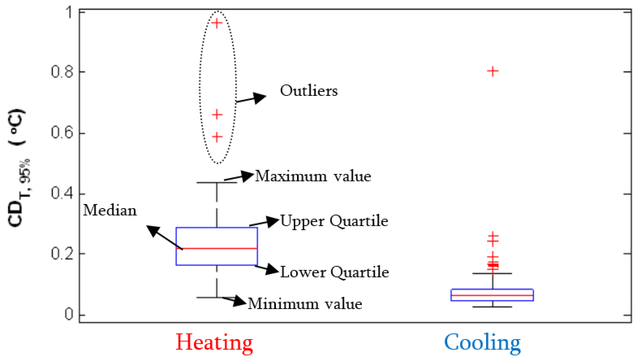
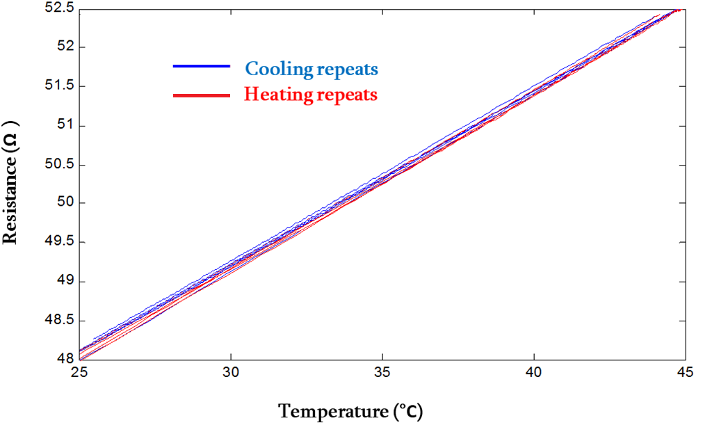
2.2. Comparison of Heating and Cooling Experiments (Single Test Repeat)

This section will present a detailed comparison between single experimental repeats of heating and cooling temperature profiles and their effect on the TR relationship. This will be realised by analysing the TR data in terms of the statistical parameters explained earlier.

Two experimental repeats, performed on a TSF sample N10046S1, were selected for comparison purposes. Here, N10046S1 stands for “sample number one (S1) of 46 inlayed structures having a sensing element of 100 µm nickel wire”. The results are presented in Figure 4, Figure 5, Figure 6, Figure 7, Figure 8, Figure 9, Figure 10, Figure 11, Figure 12 and Figure 13 and in

Table 2. Comparison of heating and cooling temperature–resistance (TR) curves in terms of statistical parameters.

Parameters	Abbreviation	Unit	Heating TR Curve	Cooling TR Curve
TR Equation	$R=MT+B$	-	$R=0.224T+42.435$	$R=0.222T+42.584$
Calibration Equation	$T=\left(\frac{1}{M}\right)R-\left(\frac{B}{M}\right)$	-	$T=4.458R-189.18$	$T=4.515R-192.25$
Test Duration	-	min	40	95
t-value	$\left(t-value\right)$	-	1.97	1.96
r-square value	$r^2$	-	0.999537	0.999993
Temperature Coefficient of Resistivity at 0 °C	${\mathsf{\alpha }}_0$	1/°C	0.0053	0.0052
Temperature Coefficient of Resistivity at 20 °C	${\mathsf{\alpha }}_{20}$	1/°C	0.0048	0.0047
Resistance Ratio (20–50 °C)	$R{R}_{\left(20-50\right)}$	-	1.143	1.141
Slope (Sensitivity)	$M$	Ω/°C	0.225	0.220
Slope Error	$S{E}_M$	Ω/°C	0.0003	0.00002
95% Confidence Interval of Slope	$M\pm C{D}_{M,95\%}$	Ω/°C	0.224 ± 0.0006 0.224 ± 0.28%	0.222 ± 0.00005 0.222 ± 0.02%
Nominal Resistance	$R_{20}$	Ω	46.92	47.01
Resistance at 35 °C	$R_{35}$	Ω	50.28	50.34
Intercept (Resistance at 0 °C)	$B,R_0$	Ω	42.44	42.58
Intercept Error	$S{E}_B$	Ω	0.013	0.0007
95% Confidence Interval of Intercept	$B\pm C{D}_{B,95\%}$	Ω	42.44 ± 0.025 42.44 ± 0.06%	42.58 ± 0.0015 42.58 ± 0.003%
Standard error in Resistance	$S{E}_{RT}$	Ω	0.034	0.003
95% Confidence Interval of Resistance at 35 °C	$R_{35}\pm C{D}_{R,95\%}$	Ω	50.28 ± 0.067 50.28 ± 0.13%	50.34 ± 0.007 50.34 ± 0.014%
95% Confidence Interval of Temperature at 35 °C	$T_{35}\pm C{D}_{T,95\%}$	°C	35 ± 0.30 35 ± 0.8%	35 ± 0.03 35 ± 0.08%

.

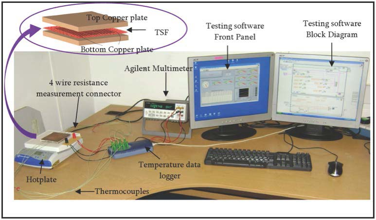
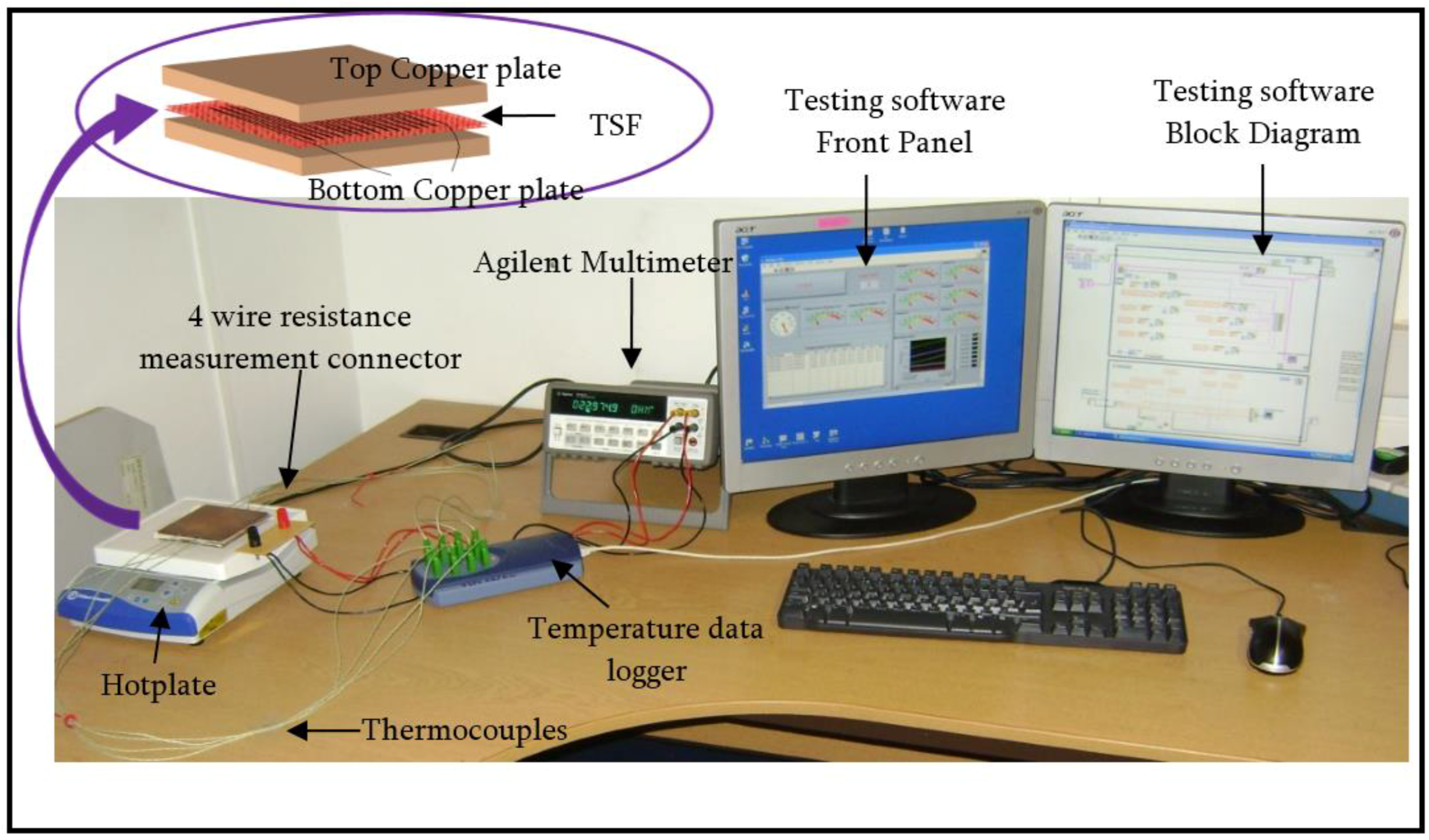
2.2.1. Testing Procedure

As explained earlier, the TR data of the TSF was measured on a customized test rig (Figure 3) over a temperature range of 20–50 °C. Initially, a TSF sample sandwiched between two Cu plates was placed on a hotplate. At this stage all components of the test rig were at room temperature. The temperature-controlled hotplate can be set to achieve a specific temperature point and maintain it. Considering the temperature range of the intended application, 55 °C was chosen as a set point of the hotplate. Therefore, heating was provided to the Cu plates in the form of a step input until the hotplate achieved its set-point temperature. The TR data were recorded by LabVIEW interface during this heating period through their respective instruments until all the components of the test rig achieved the steady state. The TR curve generated from the data during the heating phase is called the “heating TR curve”. After this, the hotplate was turned off and the rig components were allowed to cool. The difference in temperature between the rig components and the room provided a natural uniform thermal gradient. The TR curve belonging to this cooling phase of the experiment is termed as the “cooling TR curve”. The TR curves of all the experimental repeats were measured in exactly the same way. On average, the TR experiments were performed six times (three heating and three cooling) on each TSF sample.

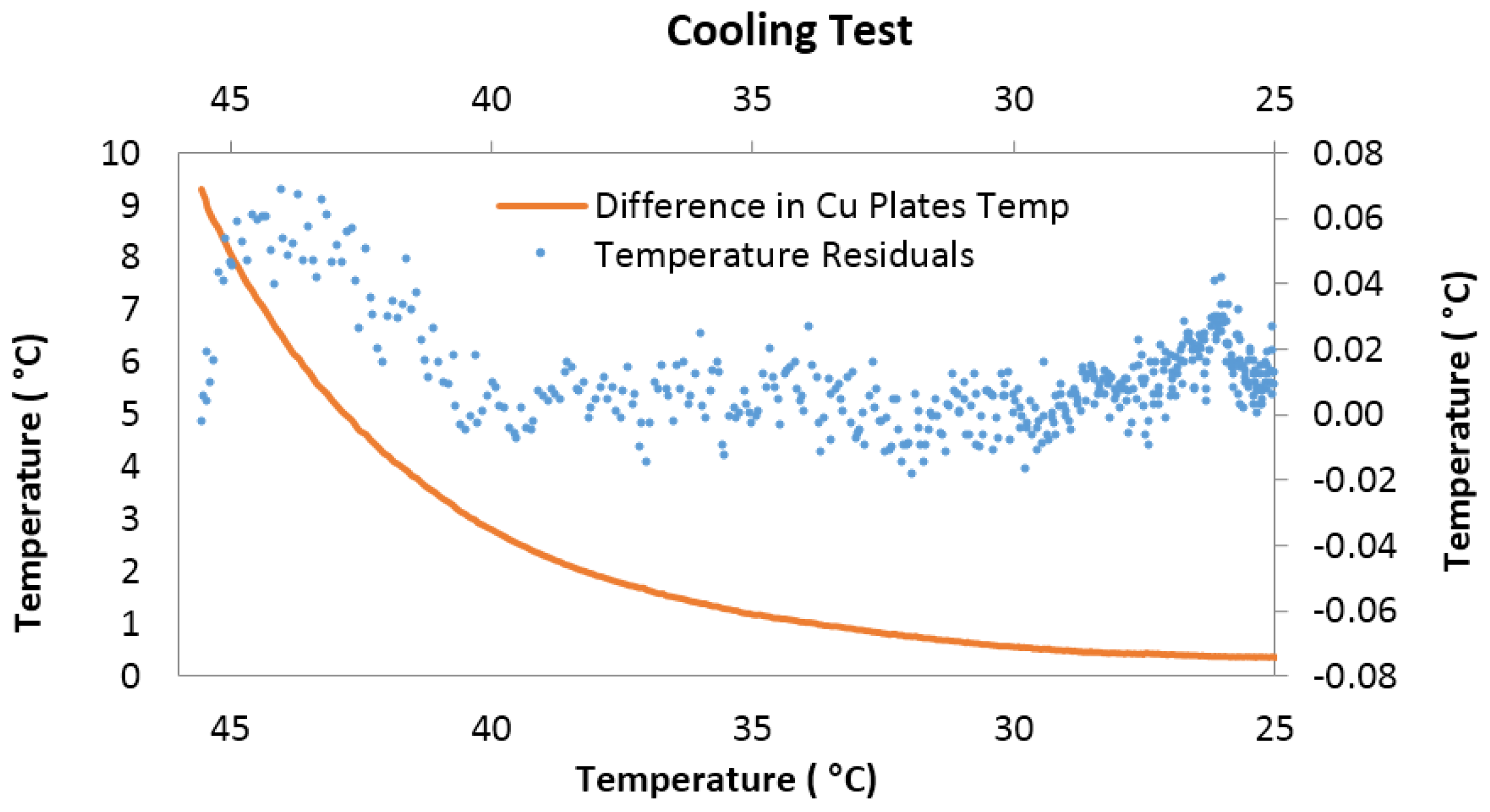
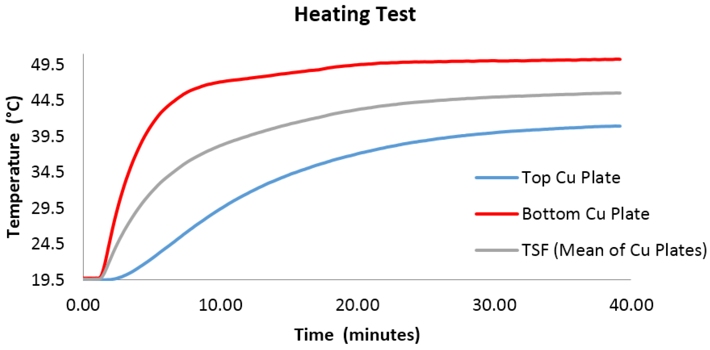
2.3. Temperature Profiles

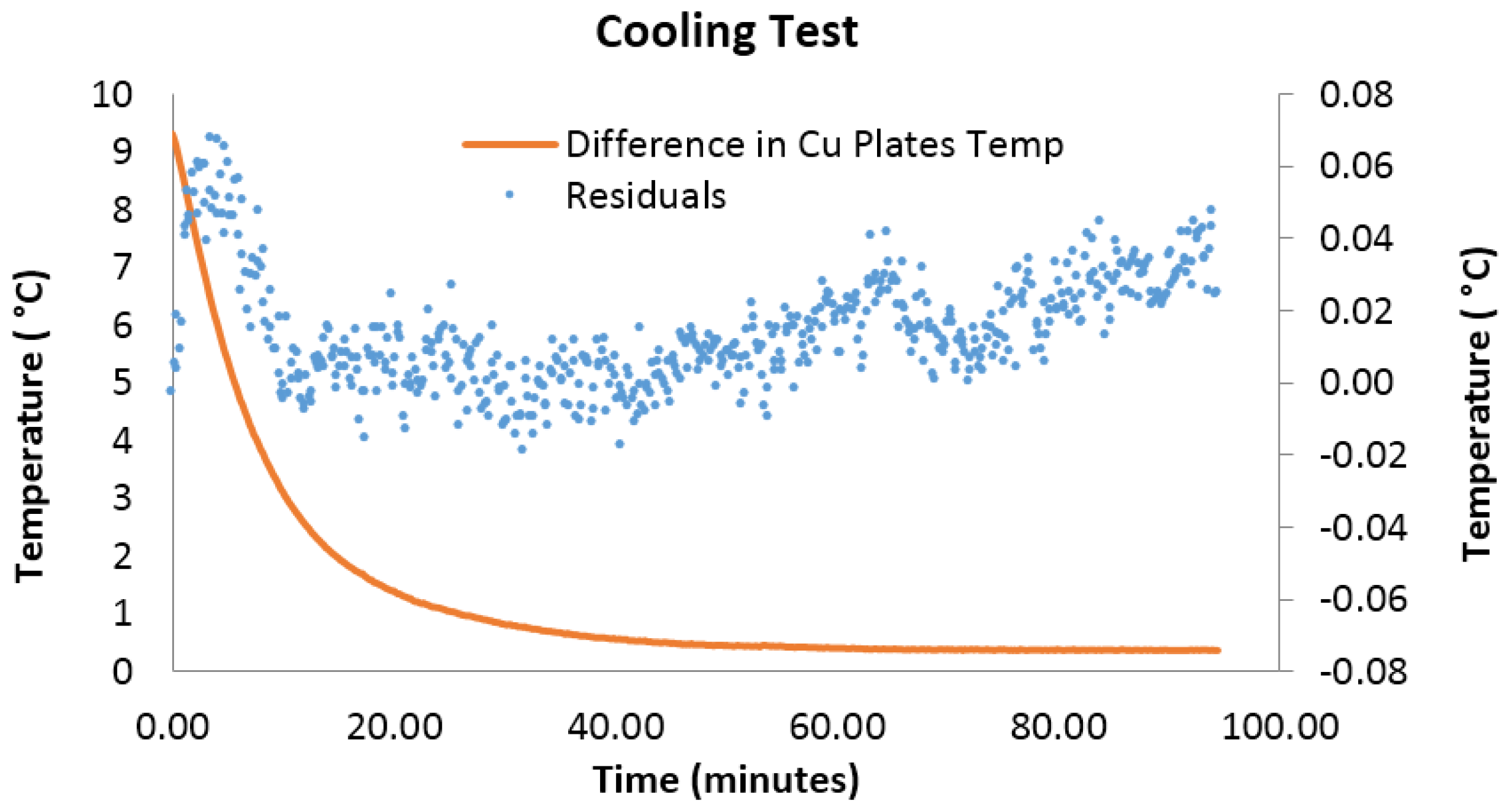
Heating and cooling temperature profiles of rig components—the bottom Cu plate, the TSF, and the top Cu plate—are shown in Figure 4 and Figure 7. As mentioned earlier, each Cu plate’s temperature was monitored with four thermocouples. This means that the presented temperature profiles of the top and bottom Cu plates are actually the mean temperature profiles of their respective thermocouples, while the temperature profile of the TSF is the average of the top and bottom Cu plate temperature profiles [7].

When the heat is applied to the rig components in the form of a step input, the bottom Cu plate increased its temperature instantaneously whilst the top Cu plate responded slightly later, as shown in Figure 4. This created a thermal gradient of around 20 °C between the Cu plates in the initial phase of heating. This difference is shown in Figure 5 and Figure 6. Figure 5 shows that the temperature difference between the Cu plates was at a maximum after around 6 min of the start of the test. At that time, the TSF had already reached 35 °C as shown in Figure 6. However, after 40 min, the rig components attained an approximate steady state. Figure 7 shows the temperature profiles of the cooling test, which lasted for around 95 min. It is important to note here that in reality, the rig components would take a lot longer than the time span described in the above tests in order to achieve a true steady-state condition. Since the recording of extra hours of experimental data would not have a substantial effect on the TR relationship, the test was stopped when the rig components achieved an approximate steady state (i.e., a condition when the rate of change of temperature with respect to time becomes insignificant). Figure 7 illustrates that the thermal gradient between the Cu plates reduces rapidly in the initial phase of cooling (first 20 min) and then approaches zero.

2.3.1. Residuals

Figure 5 and Figure 8 also present the temperature residuals of the heating and cooling test, with respect to time. Residuals were calculated from the difference between “experimental temperature data” and “fitted temperature data” at the corresponding resistance. Usually, in regression analysis, residuals are expressed on the y-axis of the graph. However, for ease of understanding, residuals have been presented in terms of temperature rather than of resistance. The majority of the residual values belonging to the heating test lie between −0.3 and 0.1. Cooling test residuals are well within the range of ±0.06. Residuals can also be represented with respect to the average Cu plate temperature as shown in Figure 6 and Figure 9. From Figure 6 it can be inferred that the majority of temperature data values arose when the test rig tried to reach equilibrium (i.e., the values lie between 40 and 50 °C). The concentration of residuals of the cooling curve is different from the heating curve. In the cooling curve, most values were recorded between 35 and 25 °C of the temperature range, as shown in Figure 9.

A slightly high residual range in the heating test can be related to the sudden initial phase of heating. These large residual values have the potential to be considered as outliers as shown in Figure 5 and Figure 6. The outliers are responsible for the skewing of the regression curve. However, it can be seen that these outliers are not large in number in comparison with the rest of residuals. Therefore, all data points were taken into consideration during the generation of the TR equation. As the rig components approached steady state, the residuals started decreasing.

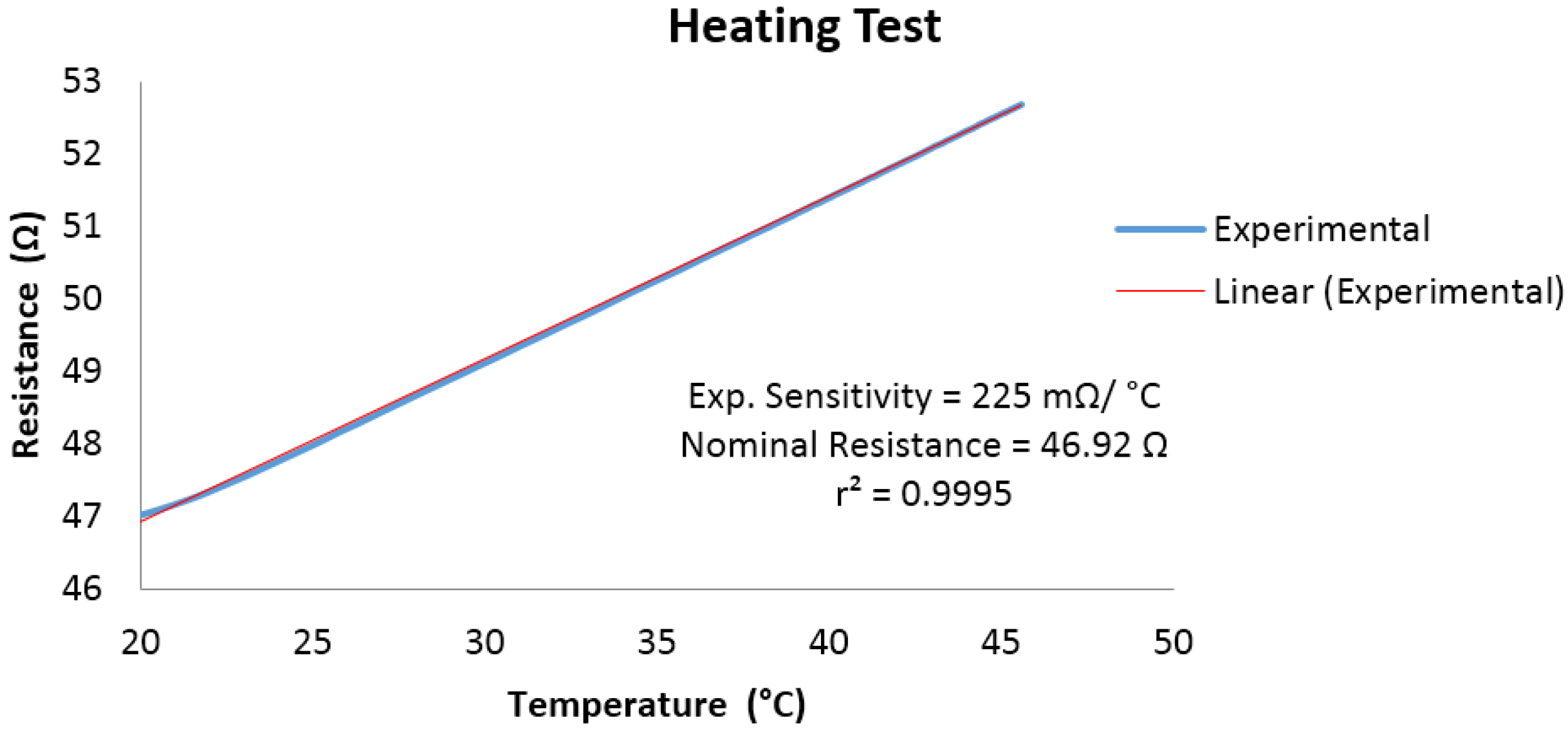
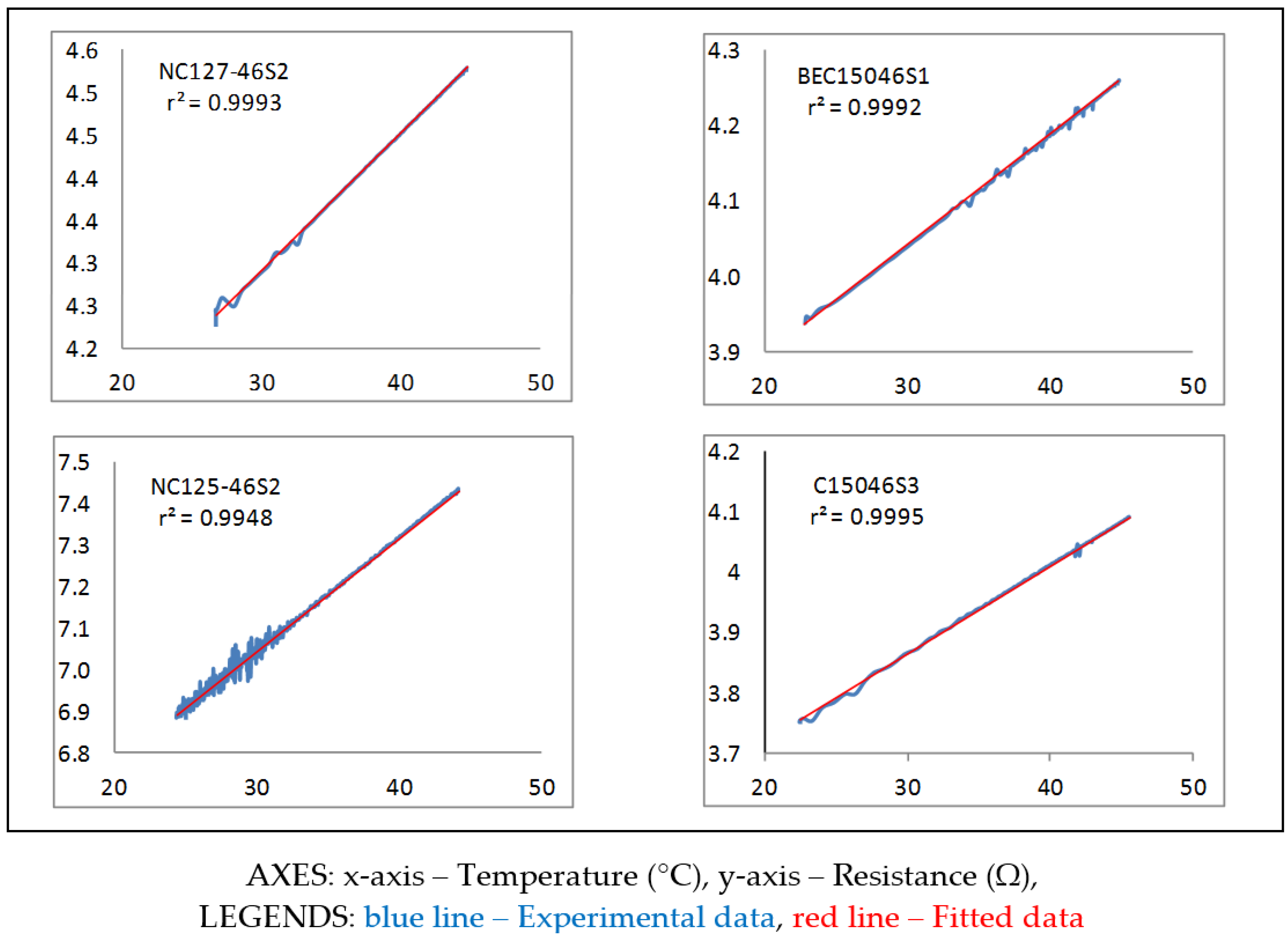
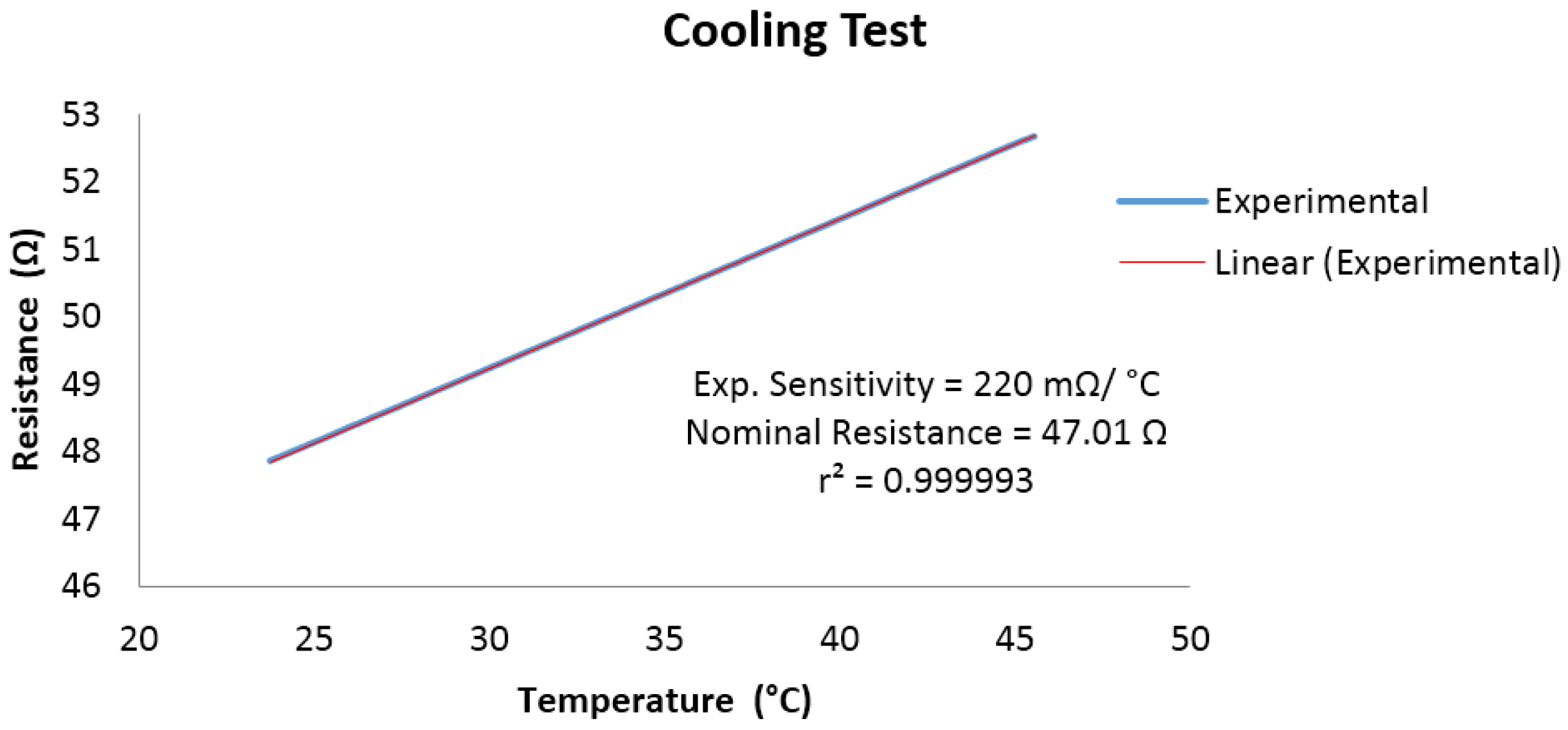
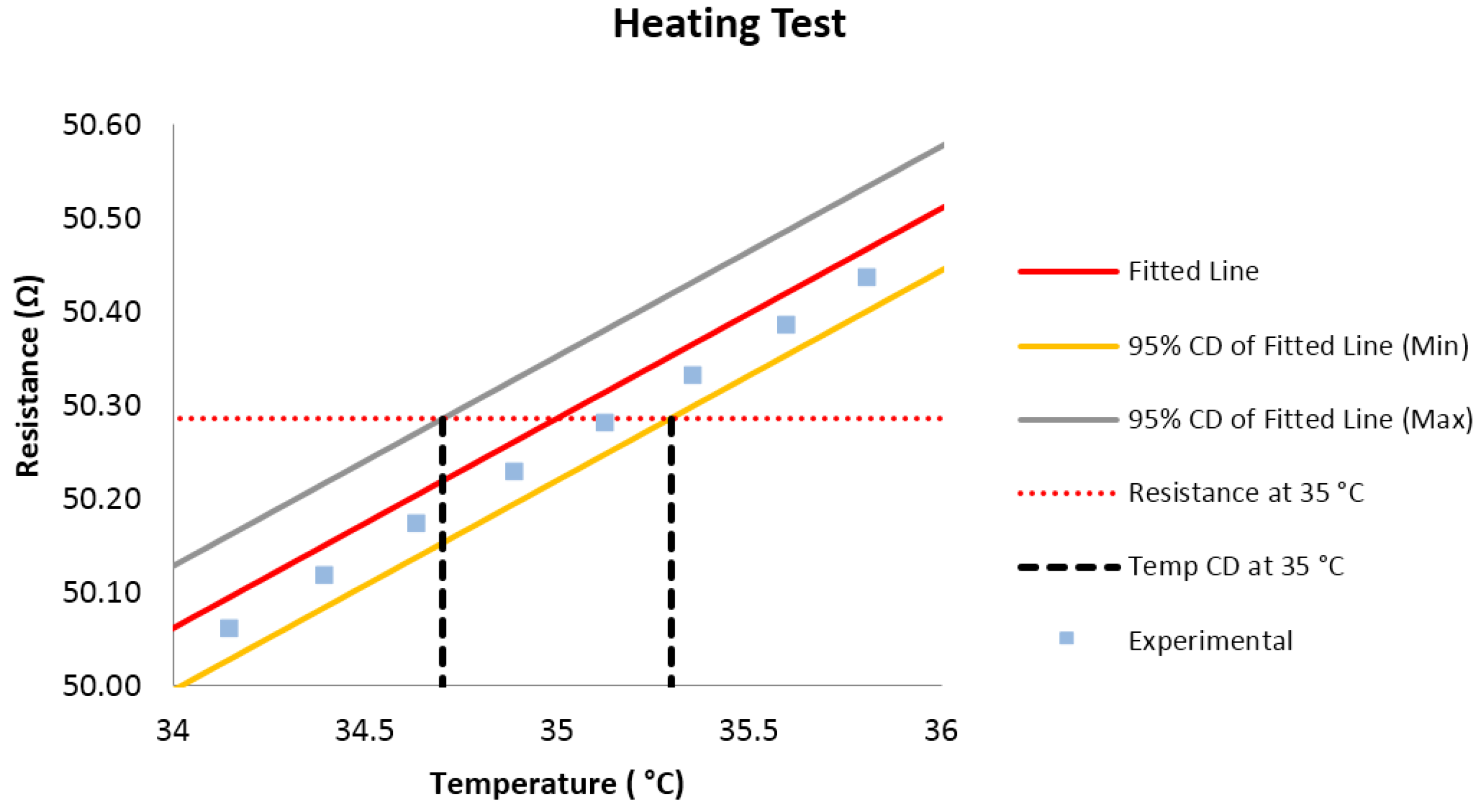
2.4. Temperature–Resistance Curves

A full range of heating and cooling TR curves is presented along with their respective fitted lines in Figure 10 and Figure 11. It can be seen that both curves seem to be identical. However, because of the sudden temperature change during the initial phase of heating (around 20 °C) phase, a slight deviation of experimental values was observed on the curve. Figure 12 and Figure 13 show magnified views of the TR curves around the region of 35°C. Moreover, the 95% confidence interval of uncertainty in resistance is also presented, along with the subsequent confidence interval of uncertainty in temperature values at 35 °C. Table 2 presents the comparative descriptions of the heating and cooling curves in terms of the statistical parameters discussed earlier.

The quality of the fitted line and its associated uncertainty can be represented in terms of standard errors and confidence deviation of resistance, slope, and intercepts. However, for ease of understanding and for purposes of comparison, it was more appropriate to estimate the uncertainties of the regression line in terms of global parameters. The 95% confidence deviation of temperature uncertainty ($C{D}_{T,95\%}$) at 35 °C is one such global parameter and shows that in the case of using a particular regression line for calibration purposes, 95% of the measured temperature values would lie within certain margins of uncertainty.

Table 2 shows that parameters related to error and confidence deviation belonging to the heating curve are higher than for the cooling curve. For example, the 95% confidence deviation of temperature $(C{D}_{T,95\%})$ of a heating curve is around ±0.3 °C; almost 10 times more than its cooling counterpart. This may be more easily visualised in Figure 12 and Figure 13.

Another global parameter which describes the quality of fitted line is the r²-value (the coefficient of determination). In accordance with other errors parameters, the r²-value of the heating curve was found to be slightly less (0.9995) than for its cooling counterpart (0.999993).

The experimental sensitivity (slope) of the heating TR curve was found to be marginally higher than that of the cooling TR curve. The same trend has been observed in alpha (${\mathsf{\alpha }}_0\mathrm{and}{\mathsf{\alpha }}_{20}$) and resistance ratio ($R{R}_{\left(20-50\right)}$) values. However, the intercept of the heating curve was found to be slightly lower than that of the cooling curve intercept. It is important to understand that the slope is an absolute parameter and depends not only upon the type and formulation of the metal of the sensing element, but on its diameter and inlay density as well. However, the alpha value ($\mathsf{\alpha }$) and the resistance ratio ($RR$) are only related to the type of metal of the sensing element. This implies that the TSF samples made with a sensing element of the same metal type (irrespective of their diameter and inlay density) would have the same $\mathsf{\alpha }$ and $RR$ values. Therefore $\mathsf{\alpha }$ and $RR$ may also be considered as global parameters while comparing the TSF samples made with sensing elements of the same metal type.

Apart from the global parameters, all remaining parameters listed in Table 2 are specific to particular experimental repeats or the TSF samples.

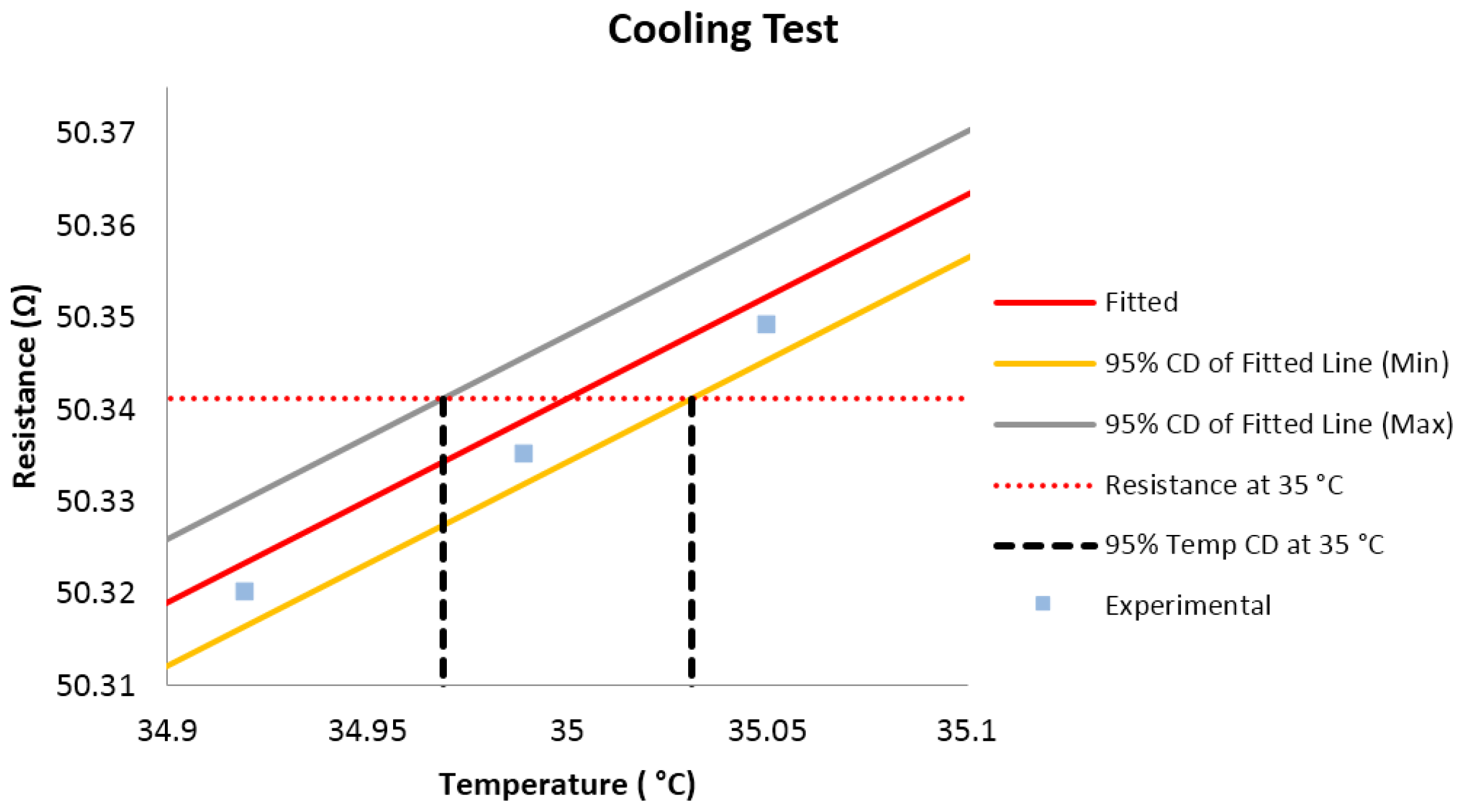
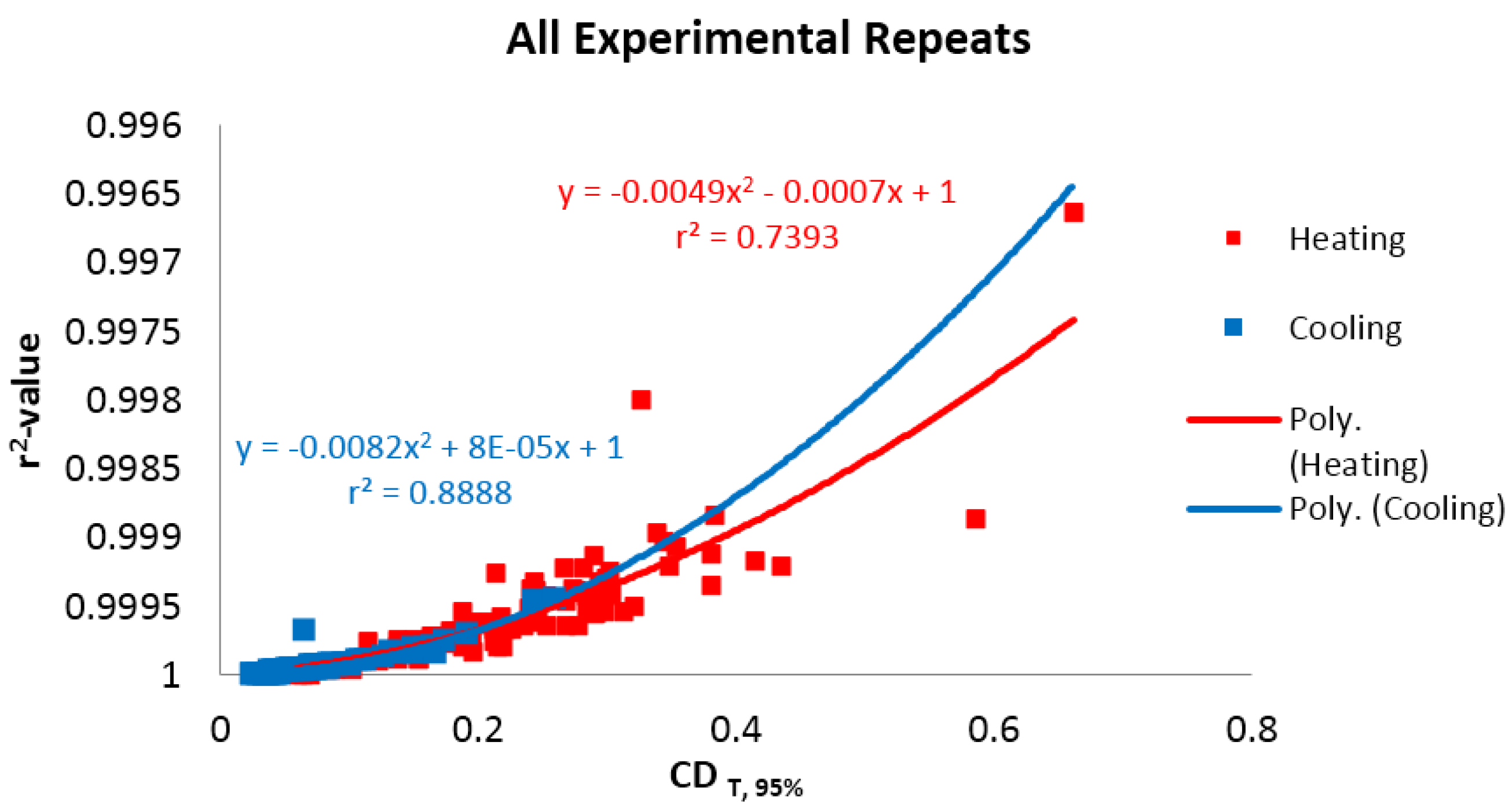
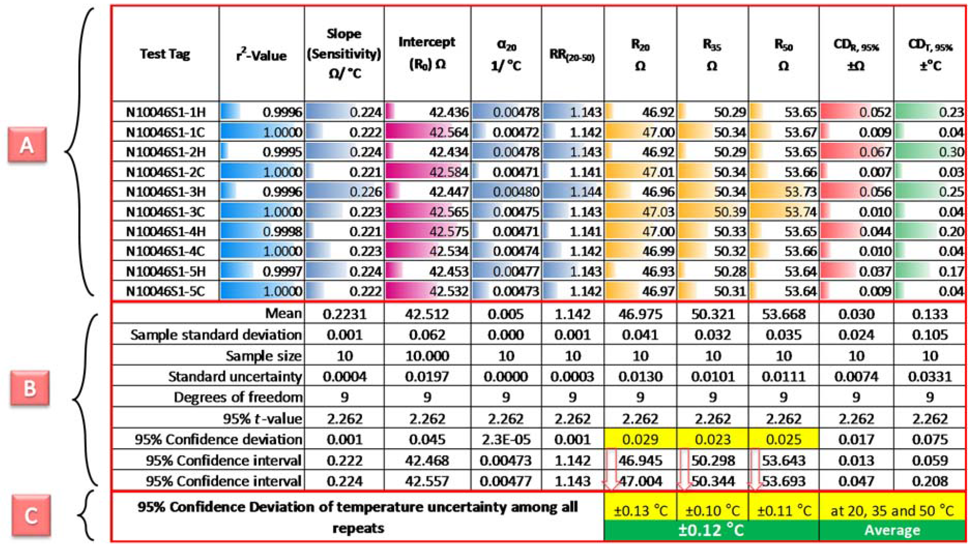
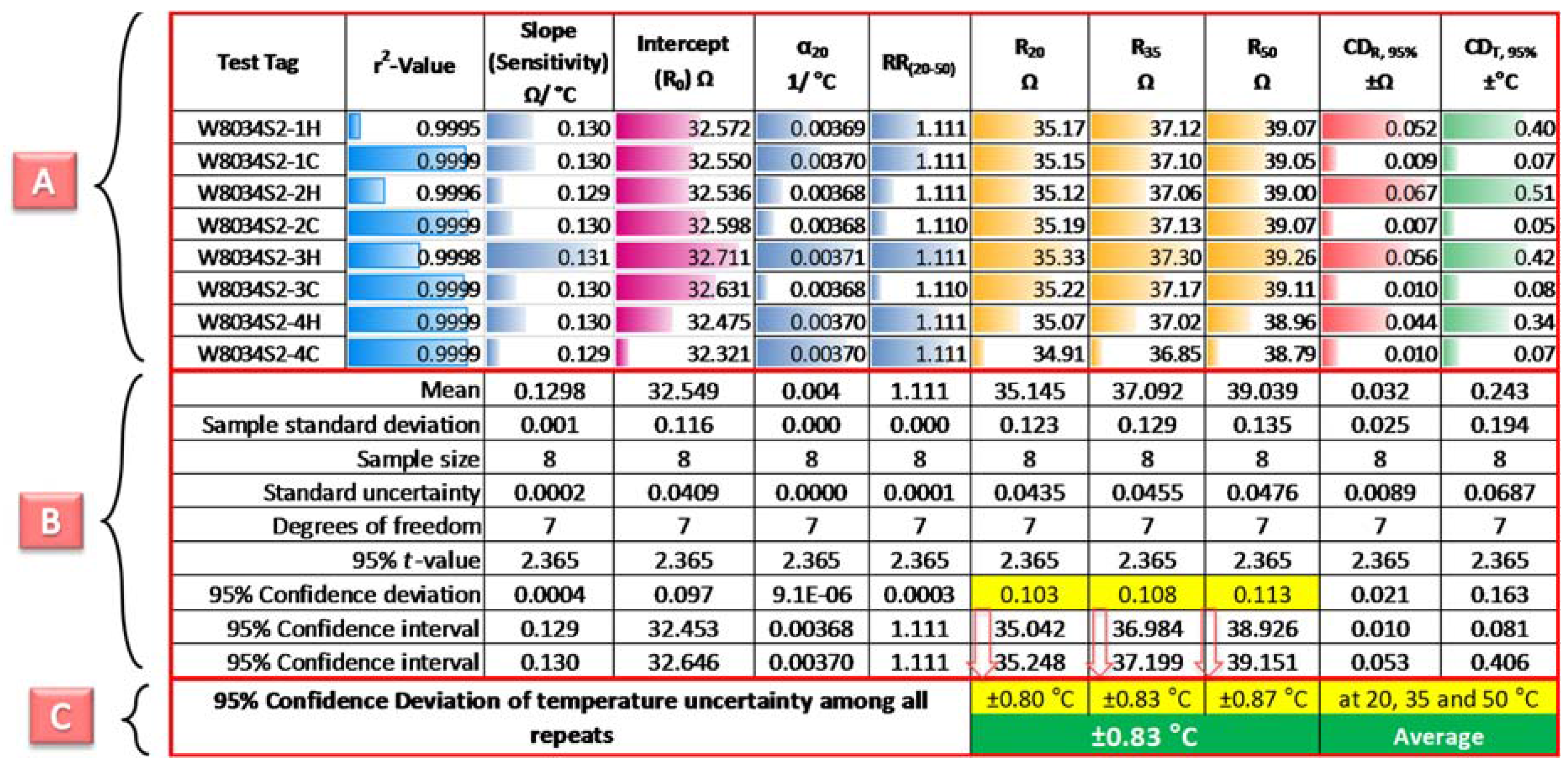
2.5. Regression Uncertainty

Regression uncertainty means the “uncertainties within repeats”. Uncertainty analysis on a single heating and cooling TR repeats have already been explained in detail. This section presents the general regression uncertainty analysis over all heating and cooling TR repeat tests by comparing them in terms of the global parameters. First, the effect of temperature profile will be discussed in detail in terms of the global variables such as the r²-value and $C{D}_{T,95\%}$. Under this heading, there will also be further discussion of the effects of the sensing element and inlay density on regression uncertainty in terms of $C{D}_{T,95\%}$. Moreover, the effects of inlay density on the experimental coefficient of temperature resistivity will also be highlighted.

3. Results and Discussion

3.1. Effect of Temperature Profile

Figure 14 presents the dispersion of $C{D}_{T,95\%}$ between the heating and cooling TR repeats in the form of a box-and-whisker plot. It is evident from Figure 14 that not only is the mean of the $C{D}_{T,95\%}$ values of heating TR repeats greater, but that the dispersion is also greater in comparison with the cooling TR repeats. Few outliers can also be seen in the cooling and heating TR repeats. Figure 15 presents the dispersion in respect of the $r^2\mathrm{value}$ of the same dataset of experimental repeats in the form (a box-and-whisker plot). The dispersion and the mean of the $r^2\mathrm{value}$ almost follow the same trend (in the opposite direction) as was discussed in the case of $C{D}_{T,95\%}$.

It may also be noted that there is an inverse relationship between the $r^2\mathrm{value}\mathrm{and}C{D}_{T,95\%}$ which can be represented in the form of a second-degree polynomial as shown in Figure 16. It can be seen that relationship between the $r^2\mathrm{value}\mathrm{and}C{D}_{T,95\%}$ of the cooling TR repeats is more predictable than in the case of their heating counterparts.

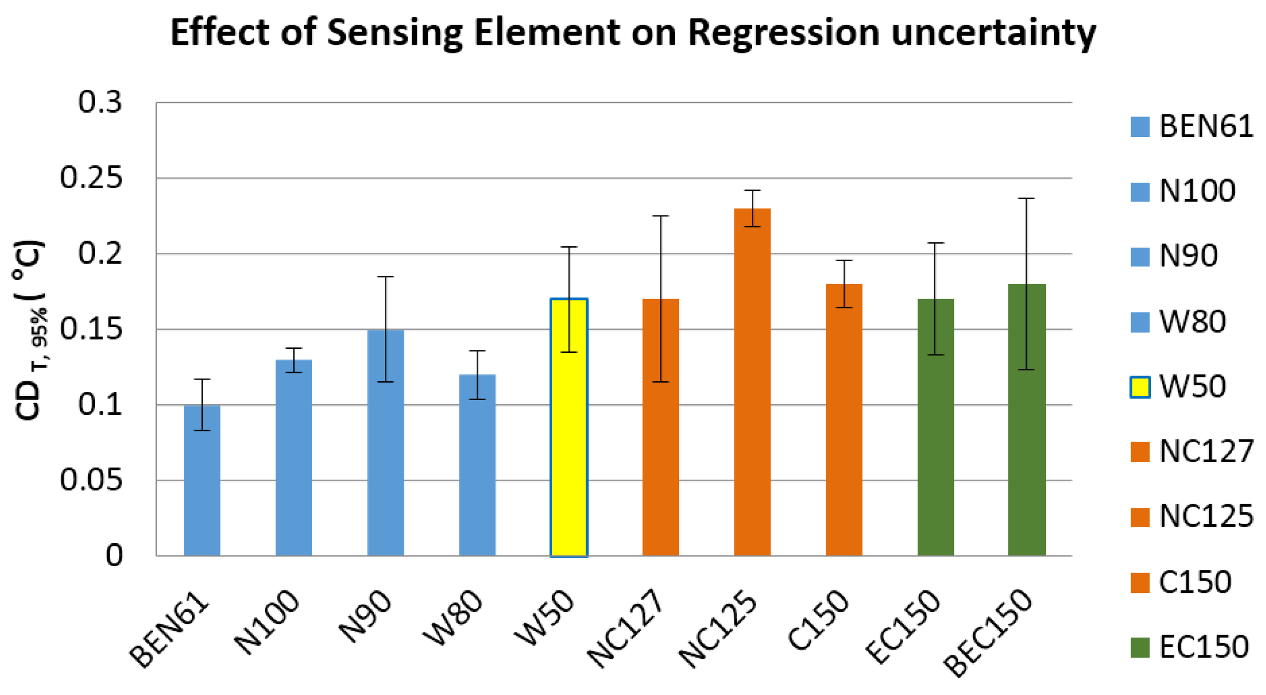
3.2. Effect of Sensing Element

Samples of the TSF were manufactured using 10 different kinds of sensing element. The TSF samples can be grouped into three ranges of reference resistance, as stated in Table 1. Figure 17 presents the effect of sensing elements on the regression uncertainty (in terms of $C{D}_{T,95\%}$). The $C{D}_{T,95\%}$ of experimental repeats of all kinds of sample were individually calculated and then grouped according to their sensing elements. The solid bar presents the mean values of $C{D}_{T,95\%}$, while the error bar presents the standard uncertainty in the corresponding group of data. The regression uncertainties in the experimental repeats of the TSF samples having high and medium ranges of nominal resistance were found to be less than ±0.13 °C, while in the case of the Cu-based TSF samples, the uncertainties exceeded ±0.18 °C, as shown in Figure 17. This marginal difference can be related to the accuracy of the multimeter.

The Agilent multimeter employed to measure resistance data was not specifically designed for high-accuracy measurement of tiny variations in resistance [30]. According to the user guide of the multimeter, measurements will always be subject to a minimum error of ±4 mΩ. For the Cu-based TSF samples, a ±4 mΩ uncertainty in resistance may contribute an error as large as ±0.3 °C. This was also evident from the graphical display of some TR repeats of the Cu-based TSF samples, as shown in Figure 18. Because of the higher reference resistance values, the TSF samples embedded with a sensing element made of Ni and W were not found to be affected by a ± 4 mΩ uncertainty in resistance, and displayed low regression uncertainty as shown in Figure 17.

The only exception to the above guideline is the behaviour of W50. Although W50 has the highest reference resistance of all the sensing elements, it still showed high regression errors. This may be related to the quality of the inlaying process of the sensing element during manufacture [5]. The TSF samples made of W50 were most difficult to manufacture because W50 demonstrated poor handling and poor bending behaviour along the edges. In some of the W50 samples, wire protruded out from the surface of the samples and may have made contact with the Cu plate during TR testing. It can be inferred that these abnormalities in W50 samples were responsible for relatively high regression errors.

The regression errors can be grouped in terms of combinations listed in

Table 3. Mean regression errors in various settings.

Group Category	Mean Regression Errors (±°C)
All repeats	0.16
All heating repeats	0.24
All cooling repeats	0.07
All repeats of 46 inlay TSF	0.15
All repeats of 34 inlay TSF	0.17
All heating repeats of 46 inlay TSF	0.22
All cooling repeats of 46 inlay TSF	0.07
All heating repeats of 34 inlay TSF	0.26
All cooling repeats of 34 inlay TSF	0.07

.

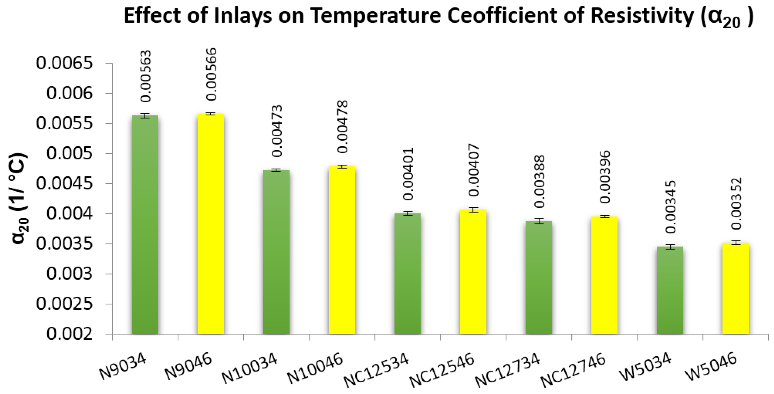
3.3. Effect of Inlay Density

The TSF samples were manufactured with either 46 inlays or with 34 inlays in a sensing area of 8 × 8 cm². Figure 19 compares the experimental values of temperature coefficient of resistivity (${\mathsf{\alpha }}_{20}$) of the 46 and 34 inlay samples within their respective categories of sensing element. It is evident from Figure 19 that the ${\mathsf{\alpha }}_{20}$ results of both groups of sample (46 inlay and 34 inlay) are the same without a significant difference.

The sensing properties of wires of the same metal type (purchased from different sources) were found to be different from the standard documented metal properties, which may be the consequence of the inclusion of impurities and differences in the wire-manufacturing process (such as work-hardening and heat treatments). For example, nickel wires from different sources were used in developing the TSF samples; they exhibited different experimental values of resistivity and temperature coefficient of resistivity.

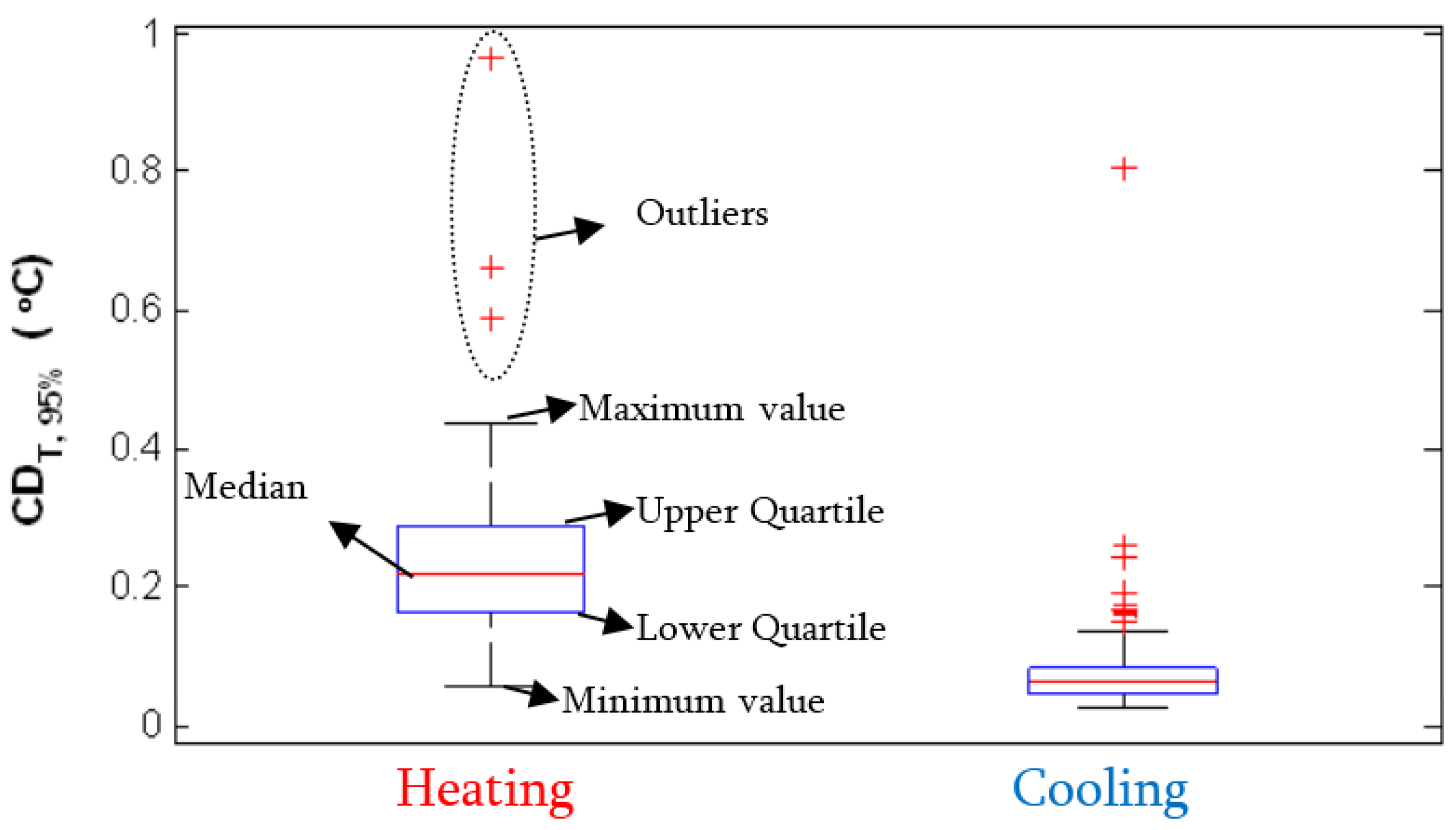
3.4. Repeatability Uncertainty

The variations within each individual experimental repeat (regression uncertainty) have been discussed. Now the repeatability of the experimental TR equation and the sources of uncertainty with respect to repeatability will be addressed. Repeatability uncertainty describes the degree to which further measurements provide similar TR data. First, experimental repeats belonging to one sample will be analysed in terms of the statistical parameters listed earlier. Then, a method to formulate the uncertainty among repeats will be devised in terms of “temperature uncertainty”. Afterwards, the analysis methodology will be extended to the full range of the TSF samples.

It also needs to be acknowledged that minor differences amongst repeated experimental cycles on the same TSF sample will exist due to variation in factors that are inherent in the TR experiment, such as testing methodology and measurement uncertainty of test-rig instruments. Experiments were performed on different days and involved pretest handling, as well. This means that the environmental conditions (room temperature and humidity), the quality of thermal contact between the TSF and the copper plates, and the quality of electrical contact between the sensing element and the 4-wire connector would be slightly different each time.

3.4.1. Analysis Criteria

The TR experiment on each sample was repeated at least six times. Various statistical parameters can be used to compare the experimental repeats of the same samples and the uncertainties-among-repeats can be estimated by the calculating the 95% confidence deviation of these parameters. For ease of understanding and for comparison, it was important to present the uncertainties-among-repeats in terms of temperature rather than as part of any resistance-related parameter. However, prior to that, it was a prerequisite to define the overall uncertainties-among-repeats in terms of resistance values across the length of the TR curve. The temperature points of 20, 35, and 50 °C were selected for the purpose of comparison. The resistance values at these temperature points (i.e., $R_{20},R_{35}\mathrm{and}{R}_{50}$) of each experimental repeat were calculated from the slope and intercept of their respective TR equations. The variations within $R_{20},R_{35},\mathrm{and}{R}_{50}$were first converted into 95% confidence deviations of uncertainty in resistance $(C{D}_{R_{20},95\%},C{D}_{R_{35},95\%,}$ and $C{D}_{R_{50},95\%})$ and then into 95% confidence deviation in temperature by dividing the $C{D}_{R_{20},95\%},C{D}_{R_{35},95\%,}$ and $C{D}_{R_{50},95\%}$ by the mean sensitivity value of each particular sample.

Table 4. Comparison and estimation of uncertainty amongst experimental repeats of TSF sample N10046S1.

presents the methodology used to estimate the variations among repeats of a sample in terms of “temperature uncertainty”. This table is divided into three sections as highlighted by the red borders. Section A of Table 4 compares the 10 experimental repeats (5 heating and 5 cooling cycles) of the TSF sample N10046S1 in terms of the r²-value, sensitivity, intercept $(R_0)$, temperature coefficient of resistivity $({\mathsf{\alpha }}_{20})$, resistance ratio $(R{R}_{20-50}),$ and reference resistances ($R_{20},R_{35},\mathrm{and}{R}_{50}$). Uncertainties within each repeat are also presented in Table 4 in terms of the 95% confidence deviation of resistance $(C{D}_{R,95\%})$ and the temperature $(C{D}_{T,95\%})$. In order to emphasise and visualise the differences within the parameter’s values, each cell of the table was highlighted in terms of colour-coded data bars. The values deriving from each parameter of experimental repeats were further analysed statistically in terms of their standard deviation, standard uncertainty, and 95% confidence deviation in section B of Table 4. The 95% confidence deviation of $R_{20},R_{35},\mathrm{and}{R}_{50}$ (i.e., ±(0.029, 0.023, and 0.025) Ω) were converted into 95% confidence deviations in temperature by dividing them by the experimental mean value (i.e., 0.223 Ω/°C), as highlighted in yellow in section C of Table 4. The 95% confidence deviation in temperature among the repeats, covering the temperature range of 20–50 °C, may be represented by one value (i.e., ±0.12 °C, by taking an average of ±(0.13, 0.10 and 0.11) °C) as demonstrated in section C of Table 4.

Figure 20 presents the TR curves of experimental repeats for sample N10046S1 as mentioned in Table 4. Heating and cooling TR repeats are drawn in red and blue, respectively.

Table 5. Comparison and estimation of uncertainty amongst experimental repeats of TSF sample W803452.

compares all the experimental repeats for sample W8034S2 and estimates the uncertainty among the repeats according to the analysis criteria discussed earlier. The 95% confidence deviation of temperature uncertainty among all repeats was calculated to be ±0.83 °C.

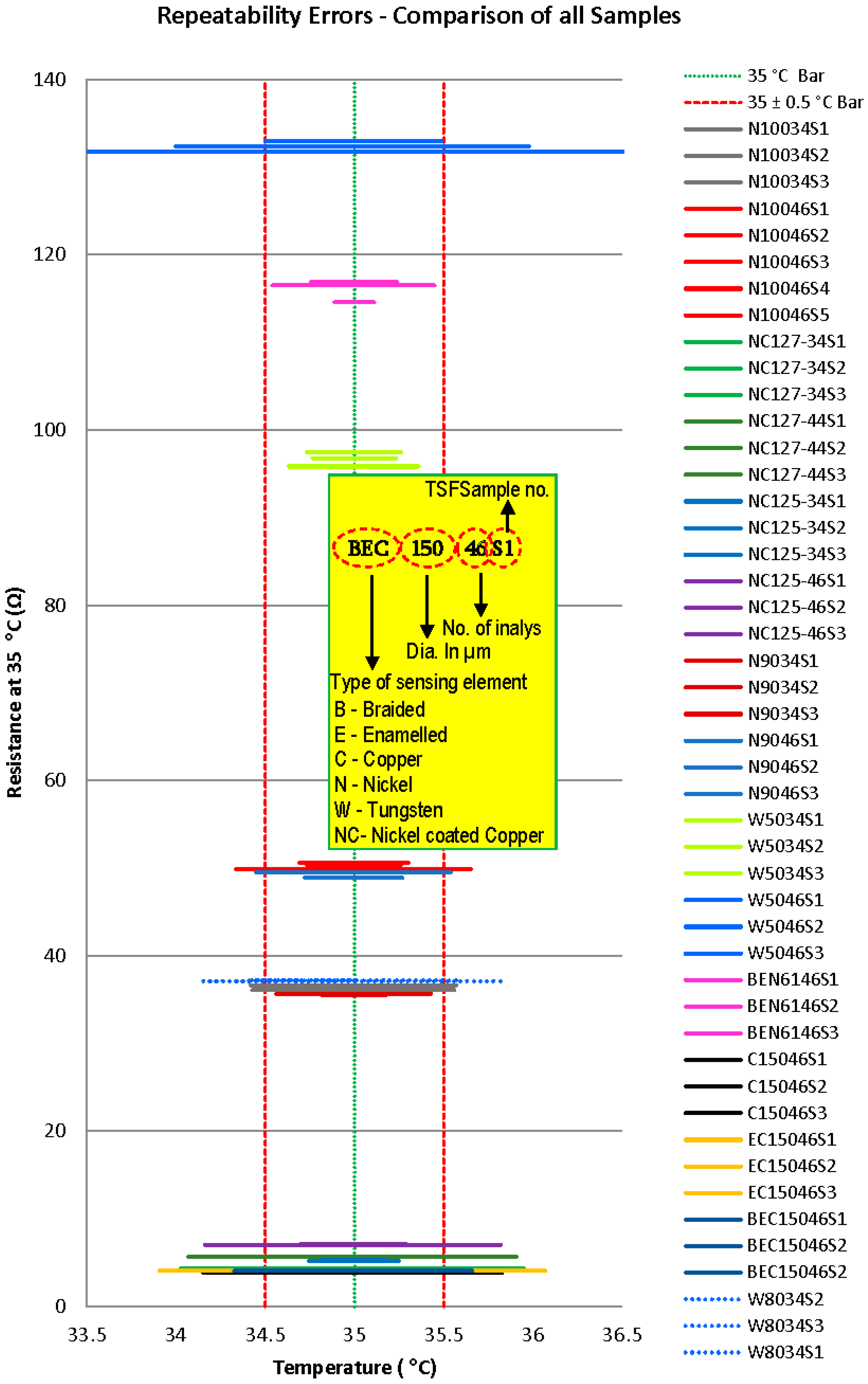
3.5. Comparison among All Temperature Sensing Fabric (TSF) Samples

The earlier-mentioned analysis criterion (calculating uncertainty amongst the repeat cycles of sample in terms of temperature uncertainty) was applied to all the TSF samples for comparison purpose. Figure 21 demonstrates the uncertainty among experimental repeats of all the TSF samples in terms of their temperature uncertainty along with their resistance values at 35 °C ($R_{35}$). The length of the bar indicates the temperature uncertainty, while the position of the bar shows the resistance values at 35 °C. It is evident from Figure 21 that the majority of samples exhibited temperature errors less than ±0.5 °C.

Some of the samples, such as W8034S2, showed quite high variations. The uncertainty-among-repeats of some of the samples were noted to be as high as ±1.5 °C. The primary reason behind such large variations in some of the samples was thought to be the connecting point between ends of sensing element and the 4-wire connector. Experimental repeats were performed on different days and required fresh connections to the 4-wire connector every time. Although care was exercised in making the connections to the sensing element at the same position, it was believed that the connecting points were slightly different during each test. Variations of ±1 cm can generate high errors in measurement by slightly shifting the reference resistance value. The connecting-point issue was resolved by attaching the dedicated Molex connector (RS Components Ltd., Corby, UK) on the TSF nonsensing area. The TSF samples having a Molex connector (such as N10046 and BEN61) showed less uncertainty among their experimental repeats (<±0.5 °C) in comparison to the rest of the samples. It can therefore be concluded that the repeatability uncertainty of the TSF samples would not be more than ±0.5 °C.

3.6. Average Temperature-Resistance (TR) Equation

In order to best represent the TR behaviour of a particular sample, its average TR equation can be generated by considering the parameters related to the experimental repeats. The average TR equation may be defined in any of the following ways:

• By considering only the three data points (i.e., the mean resistance values at 20, 35, and 50 °C);
• By considering all data points (i.e., all resistance values at 20, 35, and 50 °C);
• By considering the mean of “slope” and “intercept” of all experimental repeats.

The resultant equation would be the same, irrespective of the method applied to calculate the average TR equation. For example, in the case of the TSF sample N10046S1, the average TR equation was found to be $R=0.223T+42.512$, while in the case of W8034S2, it was $R=0.1298T+32.54$.

4. Conclusions

This article has described the investigation into the uncertainties in the TR relationship within the range of 20–50 °C with respect to the TSFs. For ease of understanding and for purposes of comparison, regression uncertainty (uncertainties-within-repeats) and repeatability uncertainty (uncertainties-among-repeats) were estimated statistically (95% confidence deviations) in terms of the temperature $(C{D}_{T,95\%})$, rather than the resistance $(C{D}_{R,95\%})$. Sometimes, global parameters were also employed to analyse results, such as the coefficient of determination ($r^2\mathrm{value}$) and the temperature coefficient of resistivity (${\mathsf{\alpha }}_{20}$). In total, more than 50 TSF samples were manufactured. A minimum of 3 samples of each type were produced, considering the inlay density and type of the sensing elements. Each sample was tested at least six times to estimate the repeatability uncertainty and to generate their TR equation.

Regression uncertainties were compared in terms of the effects of the temperature profile, sensing element, and inlay density. In all the experimental repeats, the maximum uncertainties were found to be not more than ±0.3 °C (apart from a few outliers). Uncertainties in the cooling TR equation showed considerably reduced values (±0.07 °C) in comparison with the heating TR equation (±0.24 °C). This also indicates that the test rig could be utilised to test the temperature of a TSF in a dynamic thermal environment with an uncertainty of ±0.3 °C and without any lag in its response time. Considering the multimeter’s measuring uncertainty (±4 mΩ) and the low sensitivity of copper (because of its low resistivity and its low temperature coefficient), the TSF sample made with a copper-based sensing element showed high regression uncertainty (>±0.18 °C) in comparison to the TSF sample made with a nickel and tungsten sensing element (<±0.13 °C). Among all the TSF samples, BEN61 samples (TSF made of braided-enamelled nickel wire of 61 µm diameter) showed the least regression uncertainty (i.e., ±0.1 °C). It may therefore be concluded that the TSF samples having a low nominal resistance, such as the copper-based TSF, may not be the most suitable candidates for measuring temperature in the application environment, in comparison with the higher-resistance TSF samples.

The connecting point between ends of sensing element and 4-wire-multimeter connector could considerably affect the repeatability uncertainty. A dedicated connector, such as the Molex connector, helped reduced the repeatability uncertainty from ±1.5 °C to <±0.5 °C. It can therefore be concluded that the repeatability uncertainty of the TSF samples would not be more than ±0.5 °C. It can also be concluded that the temperature and resistance values were not only repeatable but also reproducible, with only minor variations.

References

1. Funnell, R.; Koutoukidis, G.; Lawrence, K. Chapter 21—Vital Signs. In Tabbner’s Nursing Care: Theory and Practice; Churchill Livingstone: Sydney, Australia, 2009; pp. 251–274. [Google Scholar]
2. Parsons, K. Human thermal physiology and thermoregulation. In Human Thermal Environments; Taylor & Francis: London, UK, 2003; pp. 31–48. [Google Scholar]
3. Jardine, D.S. Heat illness and heat stroke. Pediatr. Rev. 2007, 28, 249–258. [Google Scholar] [CrossRef] [PubMed]
4. Ring, E.F.J. Progress in the measurement of human body temperature. IEEE Eng. Med. Biol. Mag. 1998, 17, 19–24. [Google Scholar] [CrossRef] [PubMed]
5. Husain, M.D.; Kennon, W.R.; Dias, T. Design and fabrication of temperature sensing fabric. J. Ind. Text. 2014, 44, 398–417. [Google Scholar] [CrossRef]
6. Husain, M.D.; Kennon, W.R. Preliminary investigations into the development of textile based temperature sensor for healthcare applications. Fibers 2013, 1, 2–10. [Google Scholar] [CrossRef]
7. Husain, M.D.; Atalay, O.; Atalay, A.; Kennon, W.R. Development of test rig system for calibration of temperature sensing fabric. Autex Res. J. 2017. Accepted. [Google Scholar]
8. Husain, M.D.; Atalay, O.; Kennon, W.R. Effect of strain and humidity on the performance of temperature sensing fabric. Int. J. Text. Sci. 2013, 2, 105–112. [Google Scholar]
9. Husain, M.D.; Naqvi, S.; Atalay, O.; Hamdani, S.T.A.; Kennon, R. Measuring human body temperature through temperature sensing fabric. AATCC J. Res. 2016, 3, 1–12. [Google Scholar] [CrossRef]
10. Catrysse, M.; Puers, R.; Hertleer, C.; Langenhove, L.V.; Egmond, H.V.; Matthys, D. Towards the integration of textile sensors in a wireless monitoring suit. Sens. Actuators A 2004, 114, 302–311. [Google Scholar] [CrossRef]
11. Curone, D.; Dudnik, G.; Loriga, G.; Magenes, G.; Secco, E.L.; Tognetti, A.; Bonfiglio, A. Smart garments for emergency operators: Results of laboratory and field tests. In Proceedings of the 30th Annual International IEEE Conference of Engineering in Medicine and Biology Society (EMBS), Vancouver, BC, Canada, 20–24 August 2008.
12. Derchak, P.A.; Ostertag, K.L.; Coyle, M.A. LifeShirt® System as a Monitor of Heat Stress and Dehydration; VivoMetrics, Inc.: Ventura, CA, USA, 2004. [Google Scholar]
13. Noury, N.; Dittmar, A.; Corroy, C.; Baghai, R.; Weber, J.L.; Blanc, D.; Klefstat, F.; Blinovska, A.; Vaysse, S.; Comet, B. VTAMN—A smart clothe for ambulatory remote monitoring of physiological parameters and activity. In Proceedings of the 26th Annual International IEEE Conference of Engineering in Medicine and Biology Society (EMBS), San Francisco, CA, USA, 1–4 September 2004.
14. Pandian, P.S.; Mohanavelu, K.; Safeer, K.P.; Kotresh, T.M.; Shakunthala, D.T.; Gopal, P.; Padaki, V.C. Smart vest: Wearable multi-parameter remote physiological monitoring system. Med. Eng. Phys. 2008, 30, 466–477. [Google Scholar] [CrossRef] [PubMed]
15. Soh, P.J.; Vandenbosch, G.A.E.; Mercuri, M.; Schreurs, D.M.M.-P. Wearable wireless health monitoring: Current developments, challenges, and future trends. IEEE Microw. Mag. 2015, 16, 55–70. [Google Scholar] [CrossRef]
16. Zhu, Z.; Liu, T.; Li, G.; Li, T.; Inoue, Y. Wearable Sensor Systems for Infants. Sensors 2015, 15, 3721. [Google Scholar] [CrossRef] [PubMed]
17. Atalay, A.; Atalay, O.; Husain, M.D.; Fernando, A.; Potluri, P. Piezofilm yarn sensor-integrated knitted fabric for healthcare applications. J. Ind. Text. 2016. [Google Scholar] [CrossRef]
18. Atalay, O.; Kennon, W.; Husain, M. Textile-based weft knitted strain sensors: Effect of fabric parameters on sensor properties. Sensors 2013, 13, 11114–11127. [Google Scholar] [CrossRef] [PubMed]
19. Atalay, O.; Tuncay, A.; Husain, M.D.; Kennon, W.R. Comparative study of the weft-knitted strain sensors. J. Ind. Text. 2015. [Google Scholar] [CrossRef]
20. Ziegler, S.; Frydrysiak, M. Initial research into the structure and working conditions of textile thermocouples. Fibres Text. East. Eur. 2010, 17, 84–88. [Google Scholar]
21. Bielska, S.; Sibinski, M.; Lukasik, A. Polymer temperature sensor for textronic applications. Mater. Sci. Eng. B 2009, 165, 50–52. [Google Scholar] [CrossRef]
22. De Rossi, D.; Della Santa, A.; Mazzoldi, A. Dressware: Wearable hardware. Mater. Sci. Eng. C 1999, 7, 31–35. [Google Scholar] [CrossRef]
23. Locher, I.; Kirstein, T.; Troester, G. Routing methods adapted to e-textiles. In Proceedings of the 37th International Symposium on Microelectronics (IMAPS), Long Beach, CA, USA, 14–18 November 2004.
24. Locher, I.; Kirstein, T.; Troester, G. Temperature profile estimation with smart textiles. In Proceedings of the International Conference on Intelligent textiles, Smart clothing, Well-being, and Design, Tampere, Finland, 19–20 September 2005.
25. Smartex, S.R.L. Wearable wellness system (WWS). Available online: http://www.smartex.it/index.php/en/products/wearable-wellness-system (accessed on 27 December 2015).
26. Mukhopadhyay, S.C. Wearable sensors for human activity monitoring: A review. IEEE Sens. J. 2015, 15, 1321–1330. [Google Scholar] [CrossRef]
27. Lina, M.C.; Alison, B.F. Smart fabric sensors and e-textile technologies: A review. Smart Mater. Struct. 2014, 23, 053001. [Google Scholar]
28. Lam Po Tang, S. Recent developments in flexible wearable electronics for monitoring applications. Trans. Inst. Meas. Control 2007, 29, 283–300. [Google Scholar] [CrossRef]
29. PicoTech. USB TC-08 thermocouple data logger. Available online: http://www.picotech.com/thermocouple.html (accessed on 8 December 2015).
30. Agilent Technologies. Agilent 34401A Multimeter—Product Overview. Available online: http://cp.literature.agilent.com/litweb/pdf/5968-0162EN.pdf (accessed on 8 November 2015).
31. Bell, S. A Beginner’s Guide to Uncertainty of Measurement; National Physical Laboratory: Teddington, UK, 1999. [Google Scholar]
32. Currell, G.; Dowman, A. Chapter 13—Correlation and Regression. In Essential Mathematics and Statistics for Science; John Wiley & Sons, Ltd.: Hoboken, NJ, USA, 2009; pp. 315–330. [Google Scholar]
Figure 1. A conceptual illustration of a temperature sensing fabric (TSF) embedded with braided-enamelled sensing element in double-layered knitted structure.
Fibers 04 00029 g001
Figure 2. A TSF sample of 8 cm × 8 cm sensing area along with a magnified view of the knit structure [6].
Fibers 04 00029 g002
Figure 3. A tailor-made test rig for the development of temperature–resistance (TR) curves of the TSF samples.
Fibers 04 00029 g003
Figure 4. Heating temperature profiles of Cu plates and TSF.
Fibers 04 00029 g004
Figure 5. Profile of temperature difference of Cu plates and temperature residuals of fitted curve (heating test, with respect to time).
Fibers 04 00029 g005
Figure 6. Profile of temperature difference of Cu plates and temperature residuals of fitted curve (heating test, with respect to temperature).
Fibers 04 00029 g006
Figure 7. Cooling temperature profiles of Cu plates and TSF.
Fibers 04 00029 g007
Figure 8. Profile of temperature difference of Cu plates and temperature residuals of fitted curve (cooling Test, with respect to time).
Fibers 04 00029 g008
Figure 9. Profile of temperature difference of Cu plates and temperature residuals of fitted curve (cooling Test, with respect to temperature).
Fibers 04 00029 g009
Figure 10. Experimental and fitted TR curves (Heating, N10046S1).
Fibers 04 00029 g010
Figure 11. Experimental and fitted TR curves (Cooling, N10046S1).
Fibers 04 00029 g011
Figure 12. Uncertainty in TR relationship at 35 °C (Heating, N10046S1).
Fibers 04 00029 g012
Figure 13. Uncertainty in TR relationship at 35 °C (Cooling, N10046S1).
Fibers 04 00029 g013
Figure 14. Comparison of heating and cooling TR repeats (95% confidence deviation of temperature uncertainty).
Fibers 04 00029 g014
Figure 15. Comparison of heating and cooling TR repeats (r2-value).
Fibers 04 00029 g015
Figure 16. Comparison of heating and cooling TR repeats (relationship between r2-value and CDT,95%).
Fibers 04 00029 g016
Figure 17. Effect of sensing element on regression uncertainty.
Fibers 04 00029 g017
Figure 18. Few unusual repeats of TSF samples inlaid with Cu-based sensing elements of low nominal resistance.
Fibers 04 00029 g018
Figure 19. Effect of Inlays on Temperature Coefficient of Resistivity.
Fibers 04 00029 g019
Figure 20. TR curves of experimental repeats of a TSF sample N10046S1.
Fibers 04 00029 g020
Figure 21. Repeatability uncertainty—comparison of all TSF samples.
Fibers 04 00029 g021