A Study of a Powder Coating Gun Near Field: Particle Flow in an Isothermal Staggered Concentric Air Jet

Abstract

An experimental study of inert particle dispersion in an isothermal concentric air jet near field was conducted for cases of standard non-staggered and alternative staggered jet nozzles, each taken from a polymer powder flame deposition gun. The experimental work consisted of analysis of high speed digital images of the inert two phase isothermal jet flow, illuminated by a laser light sheet along and across the jet axis. The analysis of particle spread in the jet, represented by families of particle density distributions, clearly showed that the staggered nozzles resulted in a better-focused flow, with narrower distributions in the near field, and in the elimination of the recirculation zone that disrupted the particle flow in a non-staggered nozzle arrangement. In all cases, histograms of the cross-sectional particle area density were found to be approximately Gaussian. It was also found that there was a wide variation in the size and shape of the ground polymer particles used and these two characteristics caused a wide variation in the radial and axial velocities of the particles. Despite the differences between single-phase numerical simulations and experimental results, reported in Payne et al. [1], the introduction of particles into a numerical model produced satisfactory agreement with the particle velocities found experimentally.

1. Introduction

The industrial process of polymer flame deposition consists of injecting a polymer powder into a flame created by burning air and a gaseous fuel. The goal of the process is to heat the polymer particles enough to soften them so they will adhere to the solid surface they are projected on to but not to overheat them and cause them to burn. The flame deposition process related to the work reported on here uses an air/propane flame. When the propane is turned off, the industrial equipment creates an isothermal two phase jet consisting of a coaxial air jet with inert ground polymer particles. The particles enter the air supplied to the central jet upstream of the nozzle. The quality and control of the whole deposition process depends critically upon the particle trajectories, and thus the uniformity and size of the particle jet stream all the way from the spray gun face to the target surface. In this process, the faster annular jet surrounding the particle bearing central jet serves as the main source of momentum for the particles. Control of the particle momentum is also critical for the quality of the whole process since it determines how long the polymer particles stay in the flame and thus how much each particle is heated. The aim of this study is to examine the effect of the cold coaxial air jet on the dynamics of the inert particles. This work consists primarily of finding the axial and radial velocities of the particles and their radial distributions using high-speed digital photography. A numerical simulation using Fluent is also made for comparison to the experimental results. This knowledge is part of a foundation for the successful understanding of the momentum exchange between the two phases, air and inert particles, in the field of the two phase jet.

One of the first considerations in inert two phase flow is whether the particle-particle interactions can be neglected [2] (pp. 20, 25). Whether these interactions can be neglected depends on the volume fraction of particles in the flow and the particle size distribution. In a flow with a large volume fraction of the discrete phase the particle velocities will depend in part on collisions with other particles. In the process under study here, an estimate of the particle flow rate has shown that the volume fraction of particles is about 0.05% of the volume fraction of the air so collisions between the particles can be neglected. The ratio of average particle mass flow to air mass flow is much greater, about 0.35, because the density of the ground polymer used, low density polyethylene (LDPE), is about 800 times the density of atmospheric air at room temperature. The inert nature of the flow, combined with the very low volume fraction of particles, means that there is neither volume nor mass coupling occurring in the flow.

A second important consideration is the Stokes number, defined as:

(1)

where T_v is the momentum response time of the particle and T_f is a characteristic time of the turbulent flow. The momentum response time of the particle in seconds is defined as

(2)

where ρ_d is the density of the particles in kg/m³, d is their diameter in m, and μ_c is the viscosity of the fluid in Pa·s. In practice the momentum response time of the particle, as defined by Crowe et al. [2] (p. 22), is the amount of time it takes the particle, starting from rest, to reach 63% of the velocity of the surrounding fluid. The characteristic time of the turbulent flow is most commonly defined as the lifetime of the largest vortices.

Crowe et al. [3] and Hetsroni [4] explain that if the Stokes number is much less than 1, the momentum response time of the discrete phase is much less than that of the time constant of the flow field. Then, the discrete phase flow, when it enters a turbulent vortex, will remain in the vortex and turbulent energy will be transferred from the vortex to the discrete phase through drag, decreasing the turbulence intensity of the vortex. If the Stokes number is about 1, the particle velocities will be altered only in the stronger turbulent vortices where once again turbulent energy will be transferred to them through drag. The weaker vortices will have little effect on the particles. However, if the Stokes number is much greater than 1, the momentum response time of the discrete phase is much greater than that of the time constant of the flow field and the discrete phase flow will pass through the turbulent vortices, although individual particles will show slight variations in their velocities because of a very small momentum exchange with the vorticies, as found by Mostafa et al. [5] and Mergheni et al. [6]. In this case, there will be transfer of turbulent kinetic energy to the fluid from the particles because the particles will create turbulent motion on a scale about their diameter, as suggested by Gore and Crowe [7]. When the volume particle loading is light and there is no mass exchange between phases, the Stokes number expresses the coupling of the phases in isothermal flows where there are no buoyancy effects. As the particle volume fraction increases, the increasing number of collisions between particles has a greater and greater effect on particle velocities and the applicability of the Stokes number to determination of the particle velocity decreases. Simple calculations and the experimental evidence itself show that the low density polyethylene (LDPE) particles used in this work have Stokes numbers ranging from about 1 to about 1500, depending on the size of the particles. The average Stokes number is about 120, revealing that the velocity fluctuations of the turbulent coaxial jet have little effect on most of the particles.

The effect of the turbulence of the continuous phase on particle drag has largely been studied using spheres, according to Crowe et al. [2] (pp. 92–94). In contrast, the particles used in this present work are not spherical. Crowe et al. [2] (pp. 92–94) provide evidence that as the particle shape becomes less and less spherical, the effect of drag on the particle increases.

The particle bearing coaxial jet can be thought of as an axisymmetric particle bearing jet with an annular jet added to it. A recent paper on particle bearing axisymmetric jets by Kartushinsky et al. [8] compares numerical simulations of inert, dilute two phase axisymmetric jet flow with experimental results. The paper includes numerical results of particle distributions, but does not compare these particular results with experiment.

Mostafa et al. [5] studied the case of a free coaxial jet with an annular jet that was faster than the central jet with a flow rate about 50% higher. Their geometry and flow rate were significantly different from those in this work and thus caution must be used when comparing their findings with findings here. However, their paper includes a graph showing the extent of gradual jet merging in single and two-phase cases. In both cases, the merging of two jets, characterized by a mean velocity profile with a single peak occurs around six nozzle diameters downstream from the nozzle. Payne et al. [1] found merging occurred at a similar distance for two of the three cases studied.

Mergheni et al. [6] investigated coaxial jet flows with 102–212 µm diameter glass spheres introduced in the central jet with two annular to central jet velocity ratios, 0.2 and 1.3. In the case of the slower central jet, the onset of a single peak mean axial velocity profile, indicating jet merging, was slightly beyond 10 nozzle diameters, the last profile reported. This distance is significantly longer than Mostafa et al. [5] reported.

Sadr and Klewicki [9] studied two phase flow using water jets and solid particles with a density 2.45 times that of water. Volume ratios of 0.03%, 0.06%, and 0.09%, were used so the velocities of the particles would not be altered significantly by collisions between them, as was the case in this work. Sadr and Klewicki [9] claimed that choosing particles with a density comparable to water ensured that the momentum exchange between the two phases was small enough to be negligible. The goal of their work was to study the effect of the particles on the turbulent structure of the water jets. Sadr and Klewicki [9] do not show any plots of particle distribution, limiting any comparison with the work here.

Two papers on particle air coaxial jets by Fan et al. [10,11] differed from the particle air coaxial jet examined in this work because they studied a confined air-particle jet that flowed vertically downwards, with silica gel powder as the second phase. They report using a blower at the bottom of the vertical chamber to provide suction. Fan et al. [10,11] do not discuss whether the blower could alter the jet flowfield. Laser Doppler Anemometry (LDA) was used to obtain the fluid velocities. It was found that, over the length of the jet, the particle distribution was roughly Gaussian across any jet diameter, and that the maximum radius of the particle distribution decreased with increasing particle flow. It was also found over the length of the jet that the particle axial velocity decreased with increasing radius. In contrast the present paper reports on a coaxial air-particle jet that flows horizontally and is a free jet, so it entrains the surrounding air.

Birzer et al. [12] studied a coaxial air jet with particles emanating from the central jet. Their two phase jet did not exit into still air but instead into air moving at about 8 m/s. They report that the particle distribution at any cross section of the jet is approximately Gaussian, with the distribution radius increasing with distance from the nozzles.

2. Experimental Work

2.1. Experimental Method

In the process being studied, the flame and the particle stream are created by apparatus that is described in an earlier paper by Payne et al. [1]. This apparatus includes the gun head, the component that creates the air/propane flame. If polymer particles are injected upstream into the air line that feeds the central nozzle in the gun head then a polymer particle stream through the flame will also be present. The earlier paper by Payne et al. [1] studied a coaxial air jet created by switching off the propane and the particle flow to the gun head. The current paper reports on studies of isothermal coaxial air jets bearing inert polymer particles created by one of two gun heads with the propane switched off, a gun head used earlier in the same flame deposition process, referred to here as Gun Head 1, and the gun head described by Payne et al. [1], referred to here as Gun Head 2, shown in Figure 1a,b respectively. Table 1 and Table 2 show the critical dimensions of gun heads 1 and 2 respectively. Each gun head was used to create a central air jet bearing the particles, when the particles were injected upstream into the air line feeding the central nozzle. The injection rate of the particles was not constant due in part to a wide variation in particle size and shape. This two phase central jet then mixed with a concentric annular jet to form the coaxial jets studied in the previous work of Payne et al. [1] but with the addition of the inert particles.

Figure 1. (a) Schematic longitudinal section through Gun Head 1; (b) Schematic longitudinal section through Gun Head 2.

Figure 1. (a) Schematic longitudinal section through Gun Head 1; (b) Schematic longitudinal section through Gun Head 2.

Table 1. Critical dimensions of Gun Head 1.

Dimension	Central jet	Spacing between central and annular jets	Annular jet
Radius (mm)	6.25	1.25	0.25

Table 1. Critical dimensions of Gun Head 1.

Dimension	Central jet	Spacing between central and annular jets	Annular jet
Radius (mm)	6.25	1.25	0.25

Table 2. Critical dimensions of Gun Head 2.

Experiment Number	Diameter of gun head (mm)	Approximate length of truncated central cone (mm)	Diameter of central jet (mm)	Radial width of annular jet (mm)
Experiment 1	76	14	9.5	0.38
Experiment 2				0.32
Experiment 3				0.27

Table 2. Critical dimensions of Gun Head 2.

Experiment Number	Diameter of gun head (mm)	Approximate length of truncated central cone (mm)	Diameter of central jet (mm)	Radial width of annular jet (mm)
Experiment 1	76	14	9.5	0.38
Experiment 2				0.32
Experiment 3				0.27

The experimental apparatus consisted of a high speed digital camera, a PCO 1200s, that produced 10 bit gray scale images, 1024 × 1280 pixels in size, using two lenses made by Nikon, a Nikkor 50 mm f2 and a Nikkor-Q C 200 mm f4, and an optical apparatus that created a laser sheet. In some cases, a close up lens of 1×, 2×, or 4× was used with the Nikkor 50 mm, f2 lens. The camera memory allowed it to store up to 712 full size digital images, which were then transferred to a host computer.

The apparatus that created the laser sheet, shown in Figure 2, consisted of a 0.4 W diode pumped Nd:YAG laser with a frequency doubler, producing a 1.2 mm diameter 1/e² Gaussian beam (TEM₀₀ mode) at a wavelength of 532 nm. This beam passed through a convex lens and then was projected into a 30° Edmund Scientific laser line generator that turned the beam into a planar sheet. Then the beam was reflected by a mirror 90° upwards, from the horizontal direction to the vertical direction, and into the jet flow field. In some cases a second convex lens was used to create a secondary beam waist at the jet axis, minimizing the light sheet thickness to approximately 0.5 mm at the test section and thereby maximizing light intensity. By rotating the laser line generator, the orientation of the laser sheet was changed between two options. Figure 2a illustrates the arrangement where the sheet is perpendicular to the system optical axis, while Figure 2b illustrates the in-line arrangement. The arrangements shown in Figure 2a,b were used for generating the laser sheet across the jet and along the jet axis, respectively.

Figure 2. Laser light sheet generator setup: (a) Sheet across the laser beam axis, top view; (b) Sheet in line with laser beam axis, front view.

Figure 2. Laser light sheet generator setup: (a) Sheet across the laser beam axis, top view; (b) Sheet in line with laser beam axis, front view.

The line diverged over its length, so by raising or lowering the apparatus, the length of the line was decreased or increased. Visual examination of the intensity of the line showed it was substantially uniform over most of its length, but the intensity peaked at each end over about a 1 mm length. This non-uniformity was probably due to the fact that the optical line generator was optimized for a 0.8 mm diameter Gaussian beam, and the beam used in this work was 50% larger. Since there was no other line generator available on the market the brighter ends of the laser sheet were blocked by a mask that covered about 10% of the light sheet length and this non-uniformity was thought to have no effect on the experimental work.

Later in the work, a more powerful laser diode with a 3 W beam of blue light with a wavelength of 445 nm was used to provide a better signal to noise ratio which allowed for faster shutter speeds. Faster shutter speeds were helpful in the very near field where the particle streaks overlapped at longer exposure times. This diode laser produced a beam diameter of 1.5 mm, which was converted to a sheet of laser light by passing the beam through a glass rod with a circular cross section. This laser was used to repeat the longitudinal sectional photos for all three experiments from 0 to 50 mm and from 50 mm to 100 mm, using shorter exposure times and the telephoto lens.

For the less powerful laser a narrow bandpass filter centered around 532 nm was used with the high speed digital camera. The less powerful laser sheet was placed either along the centerline of the jet or at a right angle to it. The longitudinal photos used here were all taken with the sheet concentrated into 50 mm lengths beginning at the origin of the central jet. The cross sectional photos were taken at 100 mm, 200 mm, and 400 mm from the origin of the central jet. Figure 3 shows the placement of the laser sheet and the camera for both longitudinal sectional photos and cross sectional photos.

Figure 3. Top view of the laser sheet and camera placement for (a) longitudinal photos and (b) cross sectional photos.

Figure 3. Top view of the laser sheet and camera placement for (a) longitudinal photos and (b) cross sectional photos.

Table 3 shows the particle loading is about 0.05% by volume at the nozzle. As ambient air is entrained in the jet, the particle loading will decrease further. This light loading ensures that any laser light attenuation due to particles is negligible.

Early in the work it was realized that the total exposure time of each set of 712 photos must exceed the integral time, the longest eddy lifetime, for the results to be representative of the actual flow. The estimation of the integral time relied on equations from Pope [13]. First, the dissipation was calculated using

(3)

where u_o was the macroscopic fluid velocity in the axial direction, assuming that the velocity in the orthogonal directions was negligible, and l_o was the integral length scale, in this case the diameter of the coaxial jet. Then the calculated dissipation was used to find the Kolmogorov time scale using

(4)

where ν was the kinematic viscosity of air. Finally, the Kolmogorov time scale was used to calculate the integral time scale with the equation

(5)

where Re is the macroscopic Reynolds number. This arithmetic resulted in a value for the integral length scale of about 2 ms in the very near field of the jet and about 17 ms at the downstream end of the length studied.

Table 3. The annular and central air jet properties used for experimental work with Gun Head 2.

Variable	Experiment 1	Experiment 2	Experiment 3
Annular air jet flow rate	0.10 m3/min 0.12 kg/min
Central air jet flow rate	0.04 m3/min 0.048 kg/min
Central air jet momentum at nozzle	7.52 × 10−3 N
Central air jet average nozzle velocity	9.4 m/s
Central air jet Reynolds number	6000
Estimated average particle flow rate	15 × 106 particles/min 6.3 × 10−5 m3/min 0.058 kg/min
Estimated particle loading	0.046% by volume; 35% by mass
Approximate average Stokes number	120
Annular/Central air jet momentum	25	30	35
Annular air jet momentum at nozzle	0.188 N	0.226 N	0.263 N
Annular air jet Reynolds number	2700	2700	2600

Table 3. The annular and central air jet properties used for experimental work with Gun Head 2.

Variable	Experiment 1	Experiment 2	Experiment 3
Annular air jet flow rate	0.10 m3/min 0.12 kg/min
Central air jet flow rate	0.04 m3/min 0.048 kg/min
Central air jet momentum at nozzle	7.52 × 10−3 N
Central air jet average nozzle velocity	9.4 m/s
Central air jet Reynolds number	6000
Estimated average particle flow rate	15 × 106 particles/min 6.3 × 10−5 m3/min 0.058 kg/min
Estimated particle loading	0.046% by volume; 35% by mass
Approximate average Stokes number	120
Annular/Central air jet momentum	25	30	35
Annular air jet momentum at nozzle	0.188 N	0.226 N	0.263 N
Annular air jet Reynolds number	2700	2700	2600

The minimum exposure time used in this work for an image was 50 μs, meaning that the total flow time sampled was a minimum of 35.6 ms. This total time was not continuous because of the time between consecutive images.

The irregular shape of the LDPE particles, shown in Figure 4, means that it is difficult to obtain a reliable particle size distribution. A common method of estimating the size of irregular particles is to find the diameter of the sphere that would have the same volume as the irregular particle, a method described by Jennings and Parslow [14], among others. Figure 5 shows a histogram, based on this method, of the size distribution of one sample of LDPE powder found using a Horiba LA-910 particle analyzer. It is important to realize that the exact distribution will change somewhat with each sample. The sample shown in Figure 5 is thought to be representative of the LDPE powder used in the work reported here.

Table 3 summarizes the properties of the flow from each of the two jets for each of the three experimental cases used in this work. These experimental cases were described in the previous paper by Payne et al. [1]. The same flow rates for the central and annular air jets were used with both gun heads. The same range of particle flow rates was used for both gun heads too.

Figure 4. The shapes of particles of a representative sample of polyethylene (LDPE) powder.

Figure 4. The shapes of particles of a representative sample of polyethylene (LDPE) powder.

Figure 5. The size distribution of a sample of low density LDPE Powder.

Figure 5. The size distribution of a sample of low density LDPE Powder.

2.2. Near Fields of Gun Heads 1 and 2

Figure 6a,b shows the two phase flow at the center plane of the jets from the central jet origin to 50 mm downstream for Gun Heads 1 and 2 respectively. Both digital images have been filtered to remove noise using a Matlab program summarized in the Appendix. Figure 6a shows the recirculation zone that developed in the near field of the jet produced by Gun Head 1. Gun Head 2 produced the flow shown in Figure 6b which was free of recirculation zones even though the flow rate for each jet was the same as those used with Gun Head 1.

The inward radial velocity of the annular air jet produced by Gun Head 2 caused the narrowing of the particle stream. Both figures show the acceleration of the particles as they mixed with the air originating from the annular air jet. The streaks created by particles that have been accelerated are longer than the streaks of the upstream particles that have not yet been accelerated. Experiment 3 was chosen to show these effects in the case of Gun Head 2 because it has the greatest annular air jet velocity.

Figure 6. (a) Gun Head 1: From origin of both jets to 50 mm downstream. The angled streaks in the near field show the recirculation zone in the center of the jet. Shutter speed: 400 μs. (b) Gun Head 2 (Experiment 3): From the central jet origin to 50 mm downstream. The streak brightness has been enhanced. Shutter speed: 100 μs.

Figure 6. (a) Gun Head 1: From origin of both jets to 50 mm downstream. The angled streaks in the near field show the recirculation zone in the center of the jet. Shutter speed: 400 μs. (b) Gun Head 2 (Experiment 3): From the central jet origin to 50 mm downstream. The streak brightness has been enhanced. Shutter speed: 100 μs.

2.3. Summed Longitudinal Section Images

Figure 7a–f show the result of filtering and summing a set of 712 photos for Experiments 1, 2, and 3, for 2 lengths of the jet axis: the tip of the central nozzle to 50 mm downstream of the central nozzle, and 50 to 100 mm downstream from the central jet. Note that in these photos the distances are measured from the tip of the central jet, which is about 14 mm downstream of the origin of the annular air jet. While quantitative comparison of the composite images between these three experiments is difficult, two observations can readily be made. First, none of the cases shows disruption of particle trajectories due to the presence of a recirculation volume at the air particle nozzle exit, in contrast to Figure 6a. Second, the focusing effect on the particles is most pronounced in Experiment 3, shown in Figure 7e,f because it has the highest annular air momentum.

2.4. Particle Distribution in Longitudinal Sections

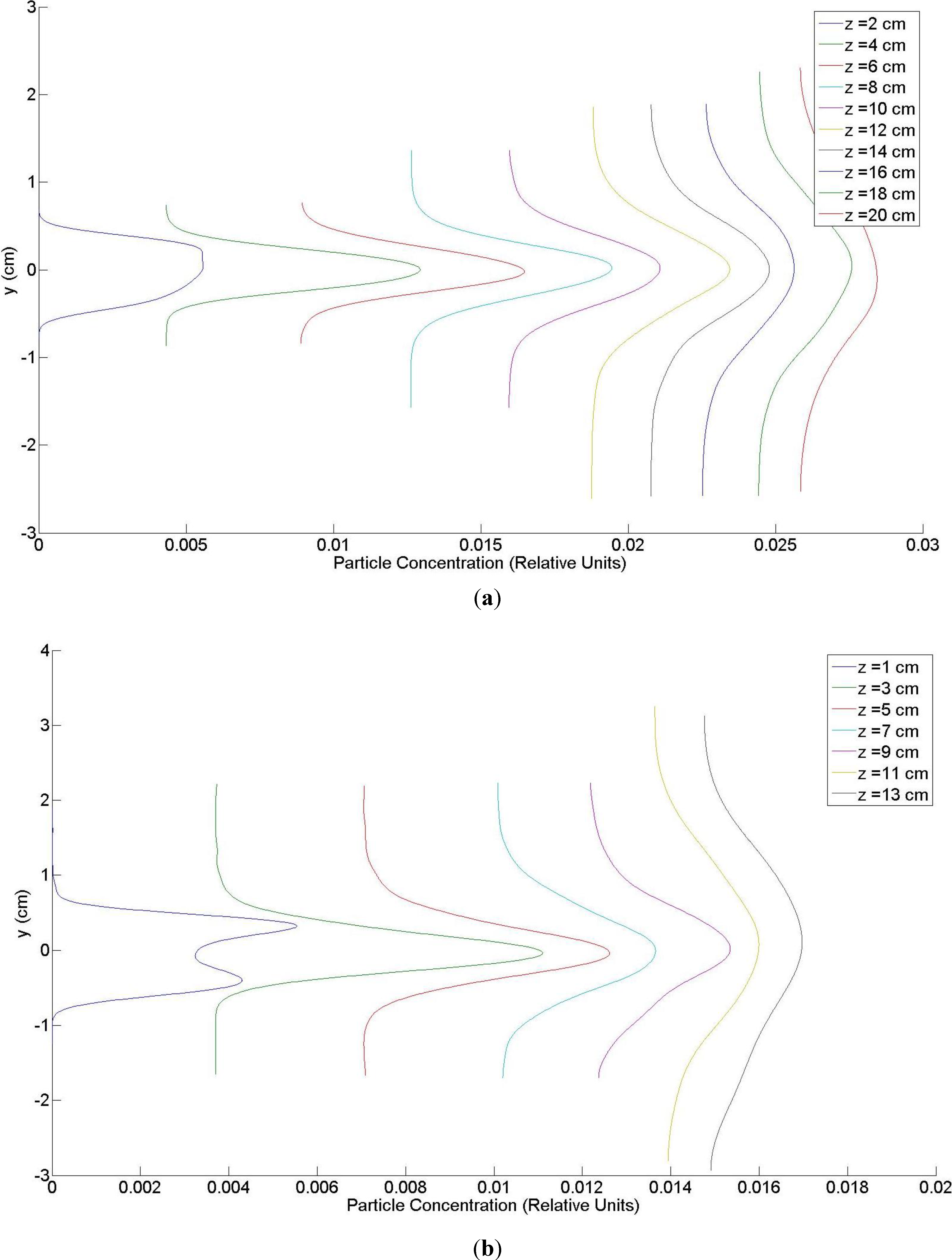
Figure 8a,b shows continuous particle concentration distributions created by Experiment 2, which used Gun Head 2, and Gun Head 1, respectively. These distributions were created using the kernel density estimation approach, also called the Parzen-Rosenblatt window method, after Parzen [15] and Rosenblatt [16] who are usually credited with its introduction. The specific implementation used here involves automatic bandwidth selection introduced by Botev et al. [17] and implemented in a Matlab program, summarized in the Appendix. The graphs show the particle distribution every two centimeters from the origin of the annular air jet downstream. In Figure 8a, the case of Gun Head 2, the first distribution curve, labeled as z = 2 cm, is located 6 mm downstream from the central jet nozzle because the central nozzle emitting the air/particle jet is itself shifted 14 mm downstream from the annular air nozzle. In Figure 8b, the case of Gun Head 1, the first distribution curve, labeled as z = 1 cm, is located 1 cm downstream from the particle nozzle since the particle stream nozzle and the annular jet nozzle lie in the same vertical plane. Data from three references, Mostafa et al. [5], Fan et al. [11], and Birzer et al. [12], have also been added to Figure 9a,b for comparison with the data gathered for this paper.

Figure 7. Sum of 712 photos from the tip of the central jet to 50 mm downstream, left images, and from 50 mm downstream to 100 mm downstream, right images. Each image spans 50 mm. Experiment 1: (a), (b); Experiment 2: (c), (d); Experiment 3: (e), (f). Exposure time: 100 μs, except (d) 200 μs.

Figure 7. Sum of 712 photos from the tip of the central jet to 50 mm downstream, left images, and from 50 mm downstream to 100 mm downstream, right images. Each image spans 50 mm. Experiment 1: (a), (b); Experiment 2: (c), (d); Experiment 3: (e), (f). Exposure time: 100 μs, except (d) 200 μs.

Figure 8. The particle distribution from longitudinal section images for (a) Gun Head 2: Experiment 2 and (b) Gun Head 1.

Figure 8. The particle distribution from longitudinal section images for (a) Gun Head 2: Experiment 2 and (b) Gun Head 1.

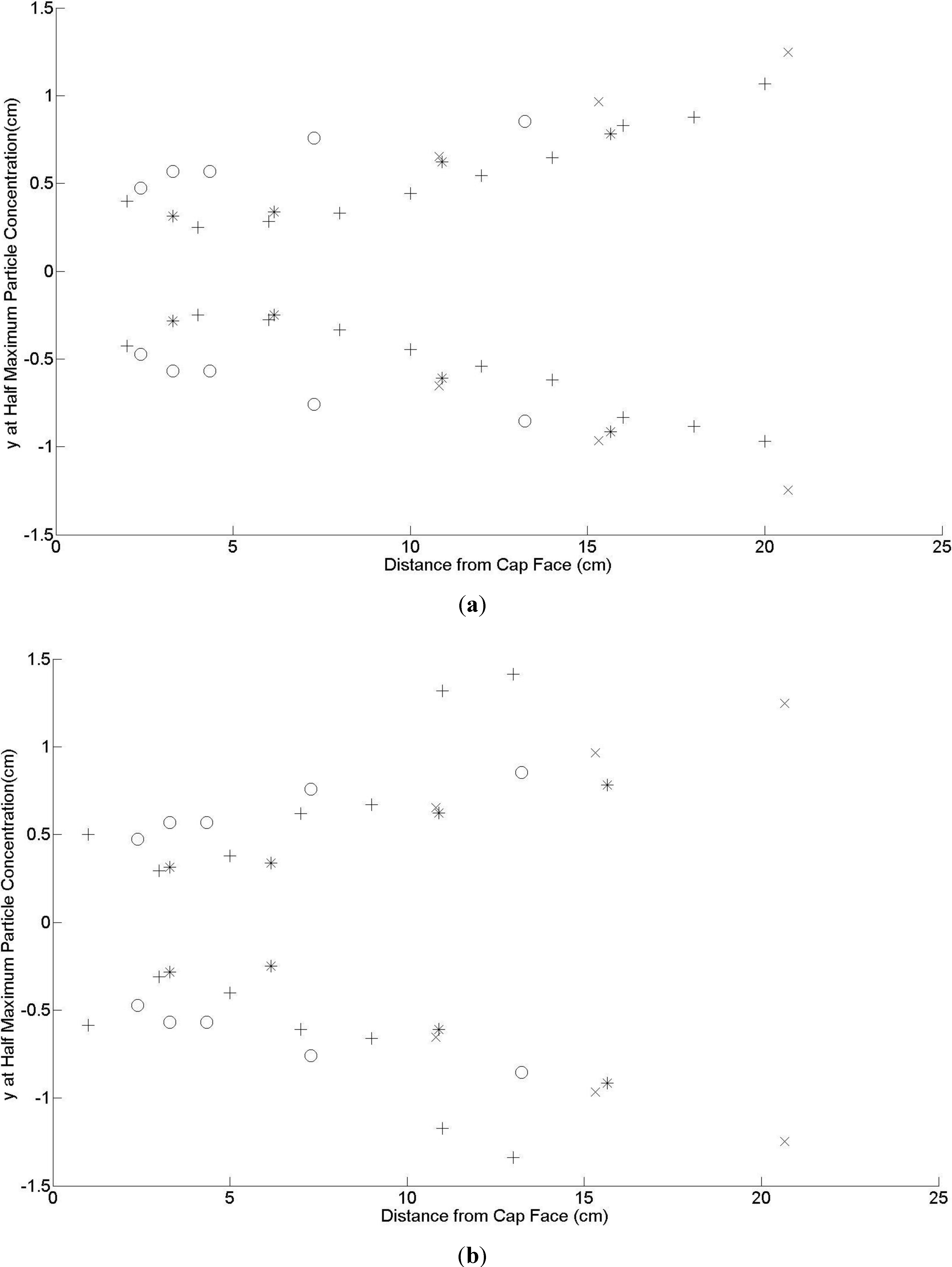
Figure 9. The radius of the particle stream at half maximum concentration and comparison with literature data: “+” present study data; “o” Mostafa et al. [5]; “×” Fan et al. [11]; “∗” Birzer et al. [12] for (a) Gun Head 2: Experiment 2 and (b) Gun Head 1.

Figure 9. The radius of the particle stream at half maximum concentration and comparison with literature data: “+” present study data; “o” Mostafa et al. [5]; “×” Fan et al. [11]; “∗” Birzer et al. [12] for (a) Gun Head 2: Experiment 2 and (b) Gun Head 1.

2.5. Particle Axial and Radial Velocities

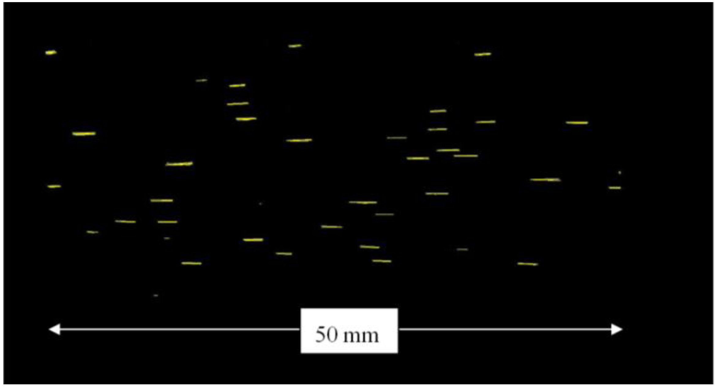
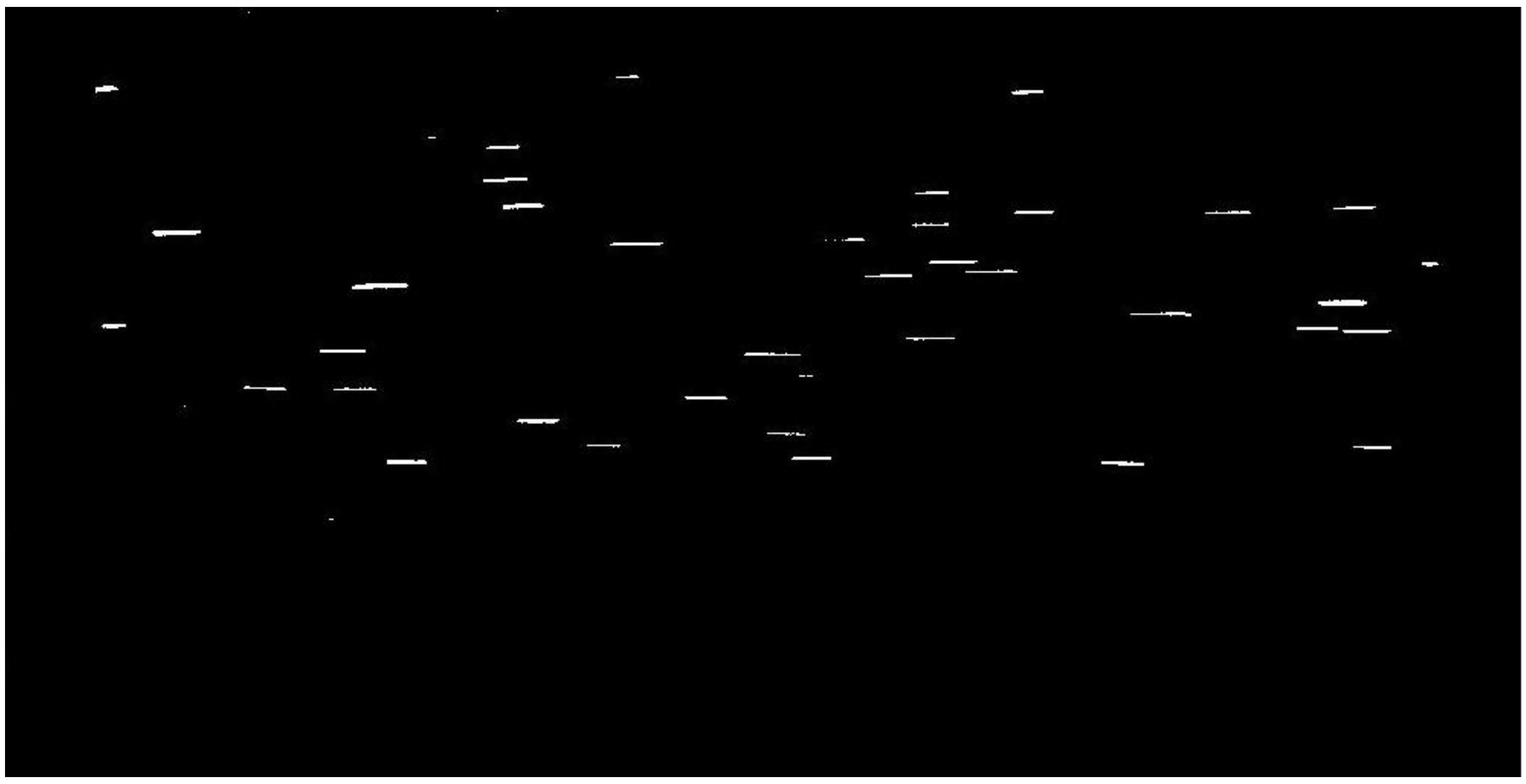
Figure 10, Figure 11, Figure 12, Figure 13, Figure 14, Figure 15 and Figure 16 show images or the results of analyzing images made by placing the laser sheet along the centerline of the jet, as shown in Figure 3a. The photographic procedure began by placing a rod with markings on it every 50 mm in the central jet. Its diameter ensured it was a slide fit in the central nozzle. This rod was photographed and used as a scale image. Then, the same length of the two phase jet was illuminated at the nominal centerline of the air/particle jet and photographed. The particles appeared as streaks, with the length and orientation of a streak being the path the particle followed while the camera shutter was open. One image from a series of 712 made using Experiment 1 settings with the laser sheet placed from 150 to 200 mm from the tip of the central jet is shown in Figure 10.

All images were made with the aperture stop of the lens in use set to maximum area. The shutter speed was then varied electronically through software that controlled the camera. It was found that while shorter shutter times meant shorter streaks and less overlap of streaks, it also meant the streaks were dimmer since less light had hit the camera CCD image detectors while the shutter was open. Thus, choosing the best shutter speed was a balance between these two conflicting factors.

These images were also found to have a significant amount of noise in them and the Matlab program, summarized in the Appendix, was used to eliminate all of the noise while removing as few of the dimmer pixels in the streaks as possible. At the same time the images were cropped at their upstream and downstream ends so each image spanned a 50 mm length of the jet. A second Matlab program, also summarized in the Appendix, was used to find the axial and radial velocity from each streak using the scale image and the shutter speed, and placed the particle at the middle of the streak. This second program created a matrix of the axial velocities and a matrix of the radial velocities from every streak in each image of every set of 712 digital images it processed. Its reliability was tested by modifying it slightly to write a yellow streak over each particle streak it detected. Figure 11 shows one such image. Comparison with Figure 10 shows this method is very reliable.

A third Matlab program, also summarized in the Appendix, found the centerline of the particle stream at the desired distance from the origin of the central jet, and extracted the axial and radial velocities for particles at this distance. These velocities were then averaged over chosen radial distances, the standard deviation of each average was found, and graphs of these average velocities, with their error estimates, were plotted as a function of the radius of the jet.

Figure 10. Experiment 1: 150–200 mm from origin of central jet. Exposure time: 100 μs. Filtered to remove noise but not cropped upstream and downstream. For scale see Figure 11.

Figure 10. Experiment 1: 150–200 mm from origin of central jet. Exposure time: 100 μs. Filtered to remove noise but not cropped upstream and downstream. For scale see Figure 11.

Figure 11. Figure 10 cropped and analyzed for particle velocities. A yellow streak was placed over the length of each particle streak the program identified.

Figure 11. Figure 10 cropped and analyzed for particle velocities. A yellow streak was placed over the length of each particle streak the program identified.

There were several sources of error in this analysis of the images made from the longitudinal illumination of the air/particle jet. The first was the removal of the fainter pixels from the particle streaks by the high pass filter that removed the noise. Every effort was made to keep this removal to a minimum. Experience showed that, at most, a few percent of the total number of streaks were significantly altered in this way, although within this few per cent were streaks that were divided into two different lengths by the removal of the fainter pixels. The second was the placement of the marks every 50 mm on the rod used as a scale. It was estimated the error in the placement of each mark was about 0.5 mm. The third was the determination of the position of the 50 mm marks in the scale photo. This error was no more than two pixels at each mark. The fourth source of error was the cropping of the images upstream and downstream. Any streak straddling the upstream and downstream borders of the image 50 mm apart would itself be cropped. Again, experience showed that only a few percent of the total number of streaks were cut during the upstream and downstream cropping of each image. A fifth and final source of error occurred when streaks overlapped. The algorithm could not separate overlapping streaks. Once again, the number of such cases was very small, by experience about 1% or 2%.

Figure 12, Figure 13, and Figure 14 respectively show the results of analyzing three sets of 712 longitudinal images each from Experiment 3. The same analysis of the longitudinal images for Experiments 1 and 2 yielded similar results, so they are not presented. The first set of 712 images included the point 10 cm from the origin of the annular air jet. The second set included the point 20 cm from the origin of the annular air jet. The third set included the point 40 cm from the origin of the annular air jet. The measuring error in the axial position was judged to be +/−0.5 mm, so the particles found to be on either side of these three distances within this tolerance were included in the analysis. The number of particle velocities found using this method usually approached 1000 so the first step in the analysis was to find the centerline of the particle flow using the positions of all of the particles over the sampled length of the flow. Next, the radius of the jet was divided into 1 mm increments from the centerline and all velocities within each increment were averaged and then plotted. 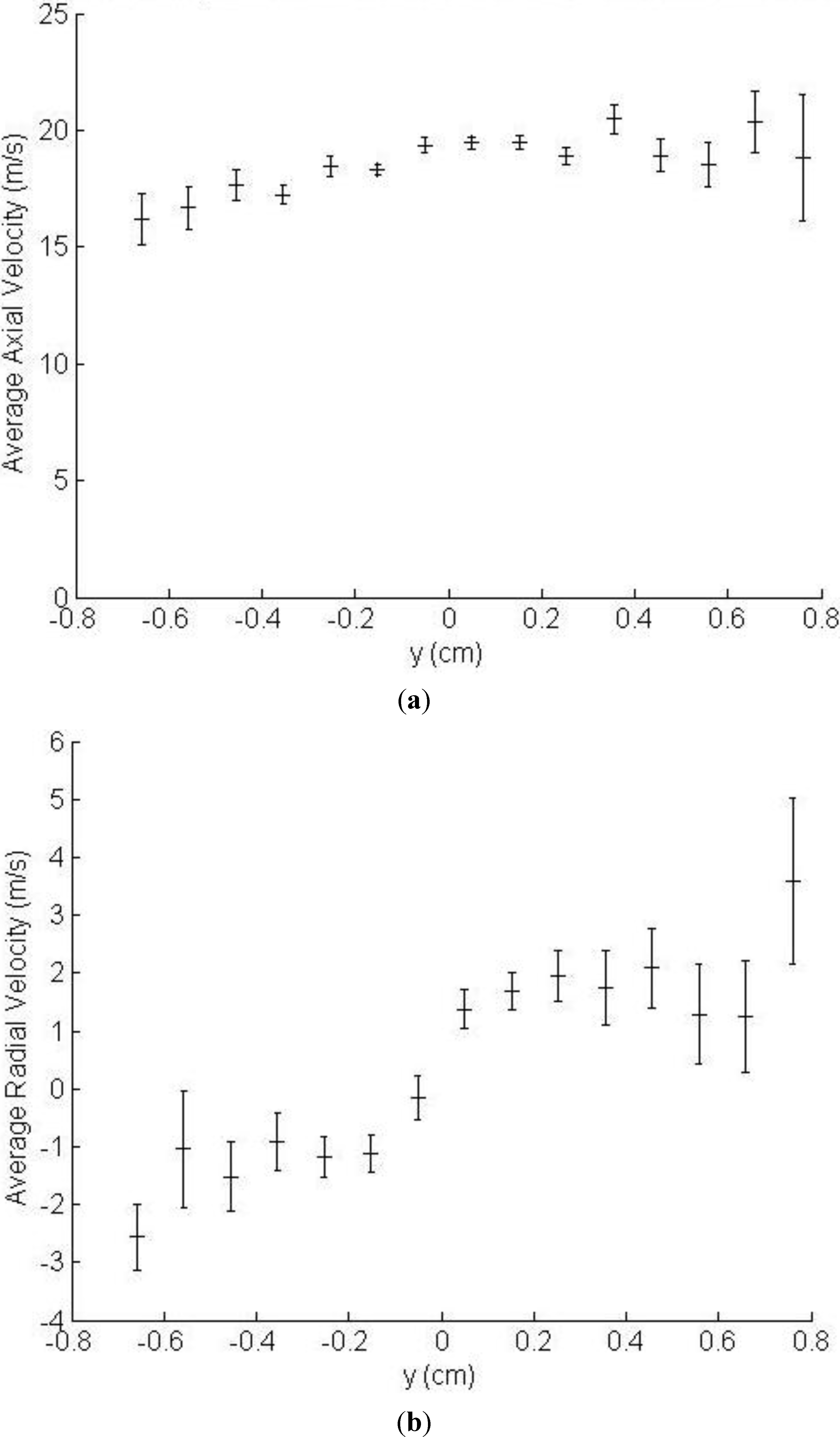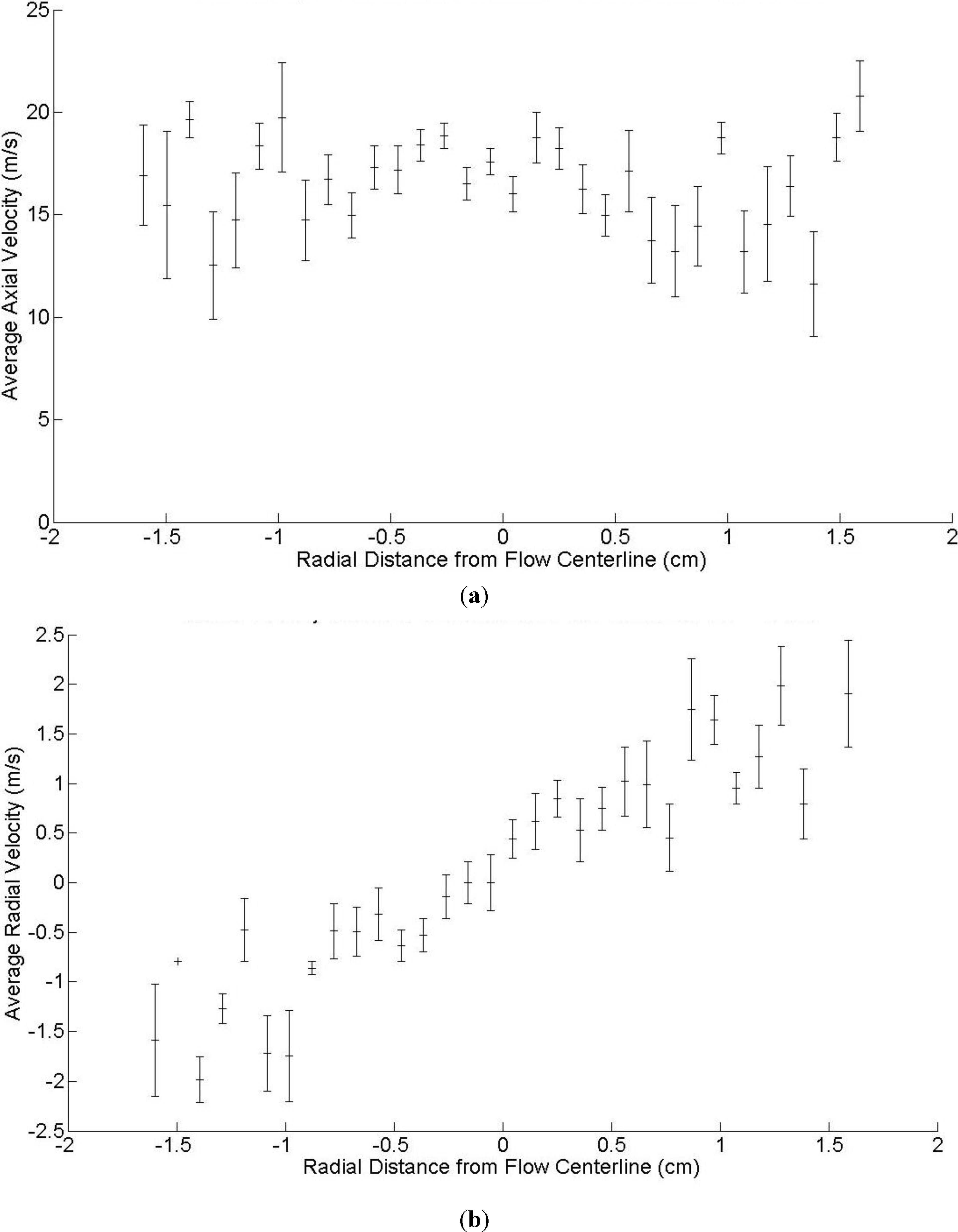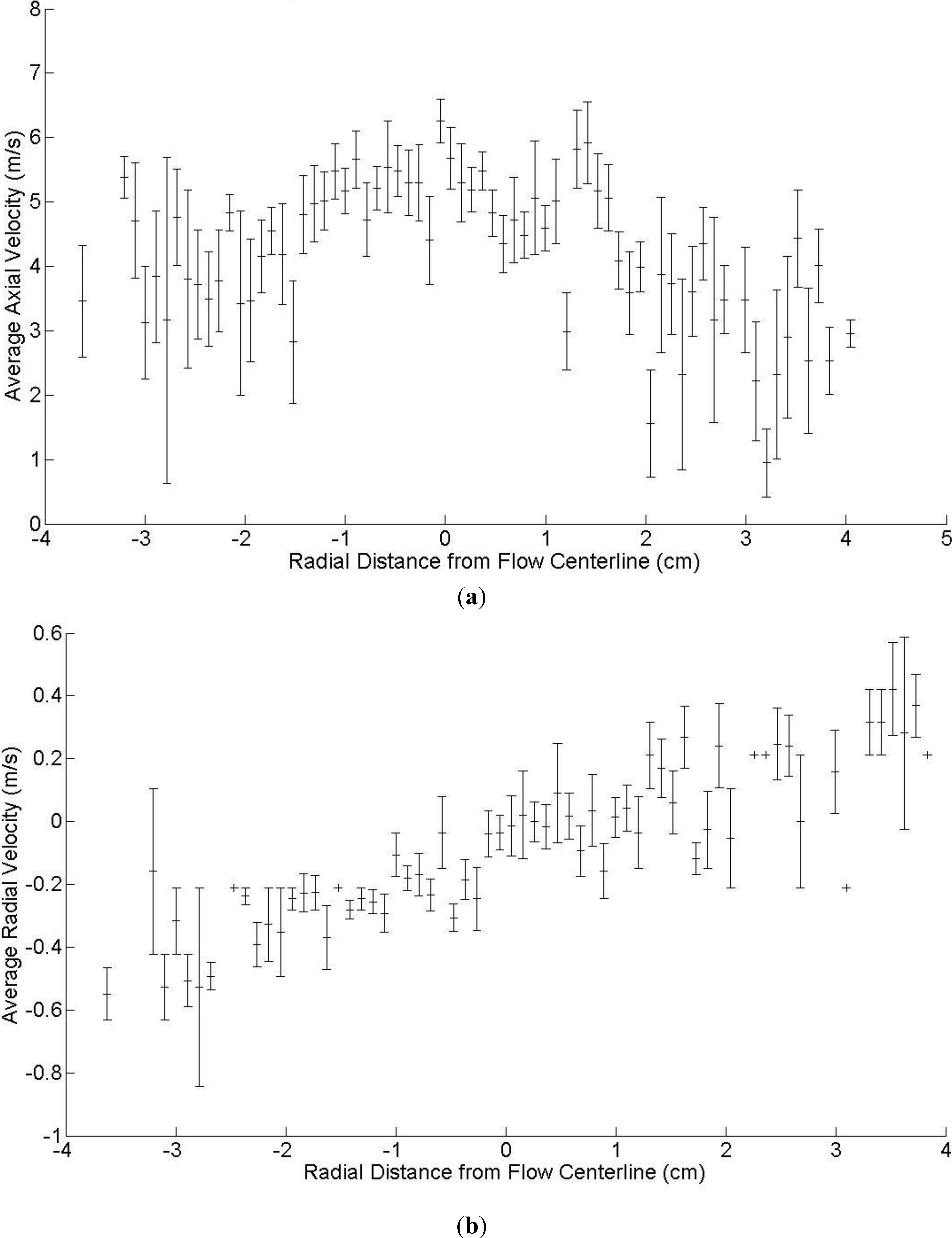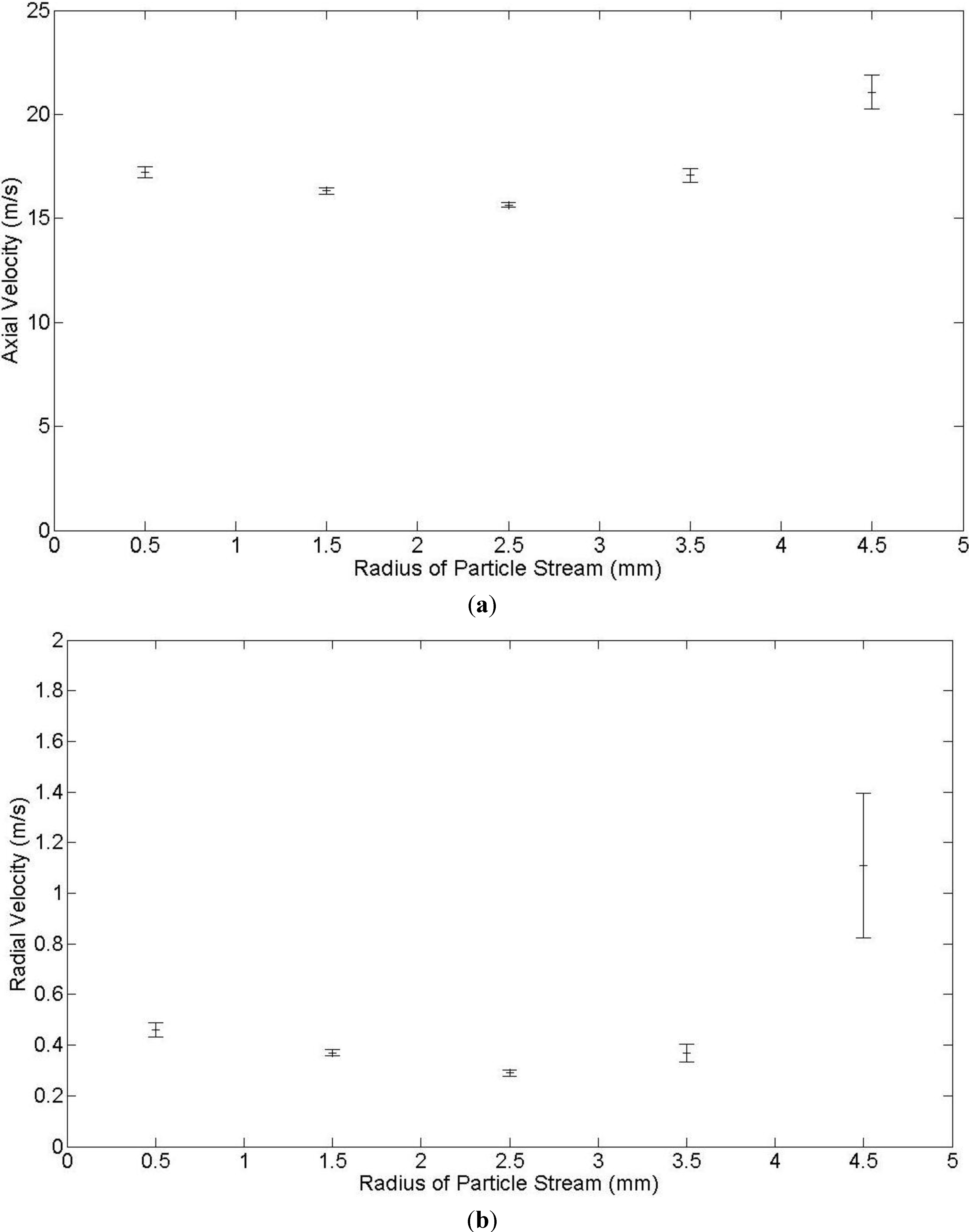Figure 12a shows the average axial velocities found using this method at 10 cm from the annular jet origin. The standard deviation of each average velocity normalized by the square root of the number of particles within that 1 mm radius is plotted as the error bar above and below that average axial velocity. Figure 12b shows the distribution of the average radial velocities, also at 10 cm from the annular jet origin. Again, the standard deviation of each average radial velocity normalized by the number of radial velocities averaged serves as the error bar above and below that average radial velocity. 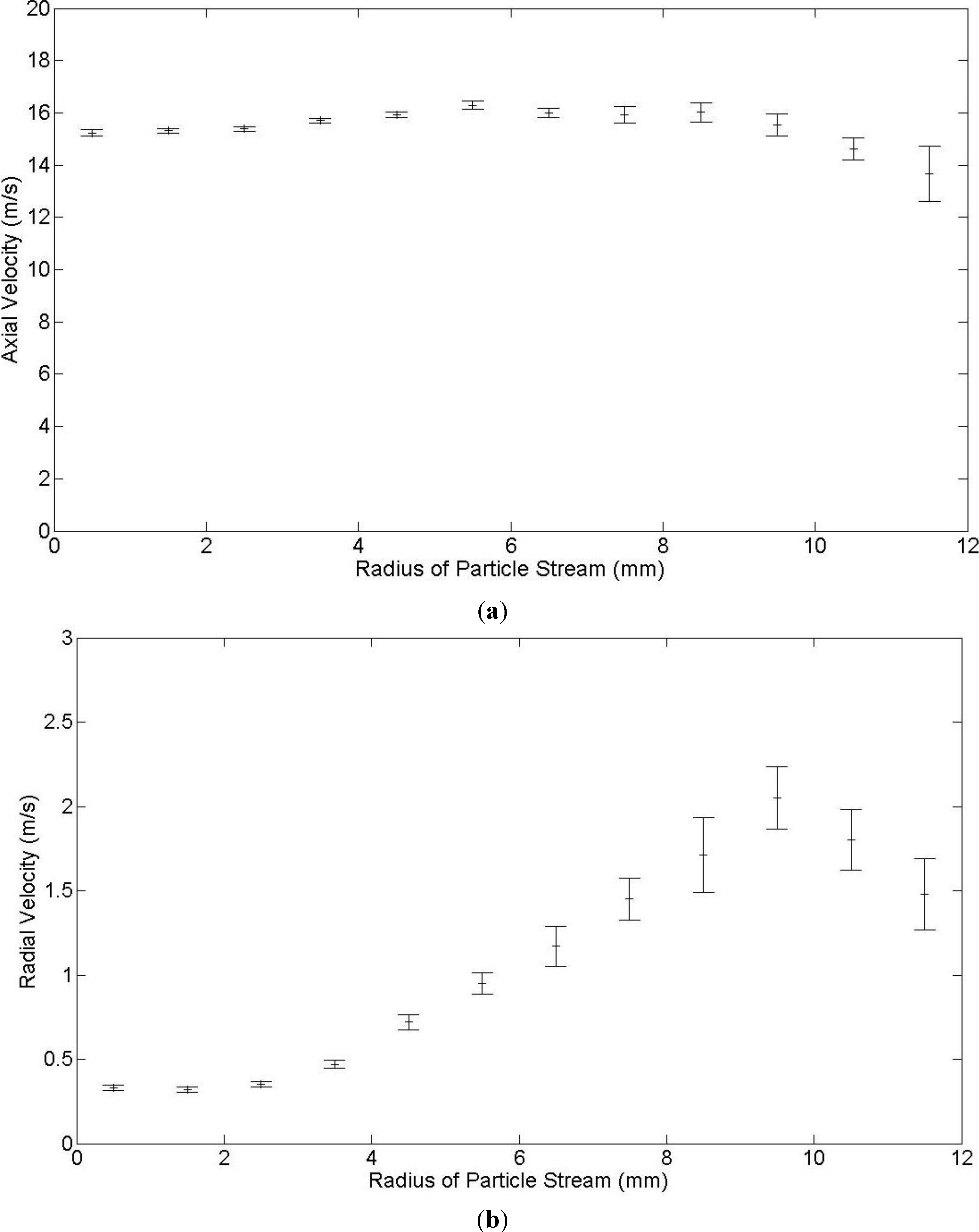Figure 13a,b and Figure 14a,b show the same results for the two phase flow at 20 cm and 40 cm respectively from the origin of the annular air jet.

Figure 12. Experiment 3: (a) Particle axial velocities and (b) particle radial velocities at 10 cm from cap face.

Figure 12. Experiment 3: (a) Particle axial velocities and (b) particle radial velocities at 10 cm from cap face.

Figure 13. Experiment 3: (a) Particle axial velocities and (b) particle radial velocities at 20 cm from cap face.

Figure 13. Experiment 3: (a) Particle axial velocities and (b) particle radial velocities at 20 cm from cap face.

Figure 14. Experiment 3: (a) Particle axial velocities and (b) particle radial velocities at 40 cm from cap face.

Figure 14. Experiment 3: (a) Particle axial velocities and (b) particle radial velocities at 40 cm from cap face.

2.6. Particle Distributions in Cross-Sectional Images

The particle distribution at several cross-sections of the flow was found by illuminating a particular jet cross-section with a laser sheet perpendicular to the jet axis and placing the high speed digital camera downstream of the cross sectional area to be photographed. The camera was not placed on the jet axis so it was not showered by particles, but instead was offset as shown in Figure 3b. The line of sight of the camera made an angle of about 10° to the axis of the jet. A set of 712 images was created for each exposure time used.

The placement of the camera off the flow centerline introduced some parallax error into each digital image. There was also a noticeable amount of noise present in each image. Consequently, each set of 712 images required some processing before the information on the radial distribution of particles could be extracted from it. Once again, a Matlab program similar to the one outlined in the Appendix was used to remove the noise from the images with a minimum loss of information. Then another Matlab program, also outlined in the Appendix, removed the parallax error from the image. Later work used the freeware program ImageJ to reduce the noise intensity by applying a “rolling ball algorithm”, followed by a Matlab program with a high pass filter set to a much lower value to remove the remaining noise.

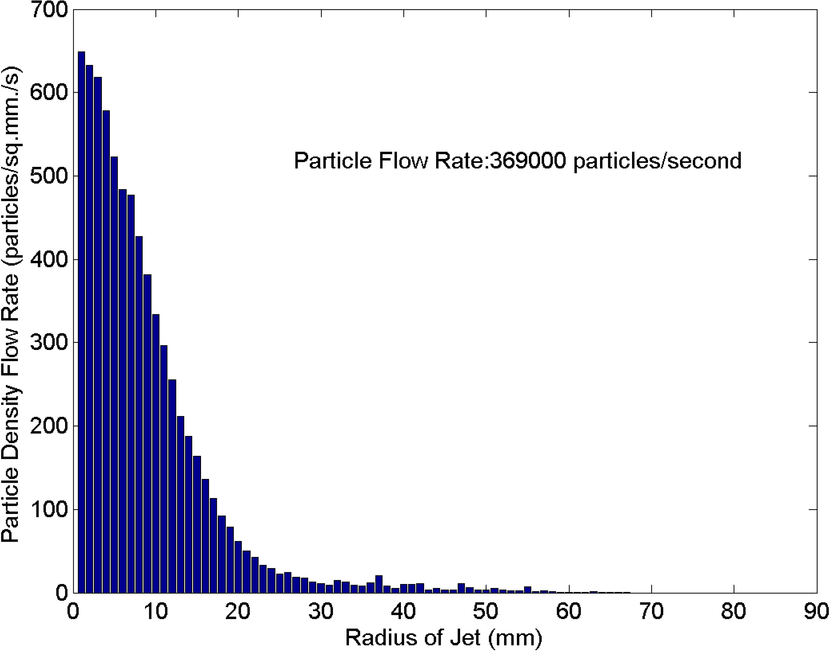
Figure 15 shows a representative image of a series of 712 taken for Experiment 1 at 200 mm from the cap face. The noise and parallax error have been removed. When each series of 712 digital gray scale images had been processed to remove the noise and parallax error, in some cases, the entire series of 712 images was summed to observe the qualitative particle distribution. Figure 16 shows one such summation. The quantitative radial distributions of the particles were obtained by sending each series of 712 images through yet another Matlab program, once again summarized in the Appendix. This program produced a histogram of the particle area density flow rate as it depended on the radius of the particle stream. The histograms for all three experiments were found to be substantially the same, so only those for Experiment 2 are shown in Figure 17, Figure 18 and Figure 19 at z = 100 mm, 200 mm, and 400 mm, respectively. It was found as the images were analyzed that the shorter exposure times yielded more meaningful images and distributions. The longer the exposure time, the more likely it was that a second particle had passed through the laser sheet at or almost at the same location as an earlier particle, resulting in the overlap of the two particle images. For longer exposure times this overlap occurred often enough that it had a deleterious effect on the results of the analysis of the radial distribution of the particles.

Figure 15. Experiment 1: One image at 20 cm from the cap face filtered, with parallax removed. Exposure time: 200 μs. The dispersed distribution of the particles in a cross section of the air/particle jet 100 cm square.

Figure 15. Experiment 1: One image at 20 cm from the cap face filtered, with parallax removed. Exposure time: 200 μs. The dispersed distribution of the particles in a cross section of the air/particle jet 100 cm square.

Figure 16. Experiment 1: Sum of a series of 712 images, each filtered, with parallax removed, at 200 mm from the cap face. The summed images show a cross section of the air/particle jet 100.0 cm square.

Figure 16. Experiment 1: Sum of a series of 712 images, each filtered, with parallax removed, at 200 mm from the cap face. The summed images show a cross section of the air/particle jet 100.0 cm square.

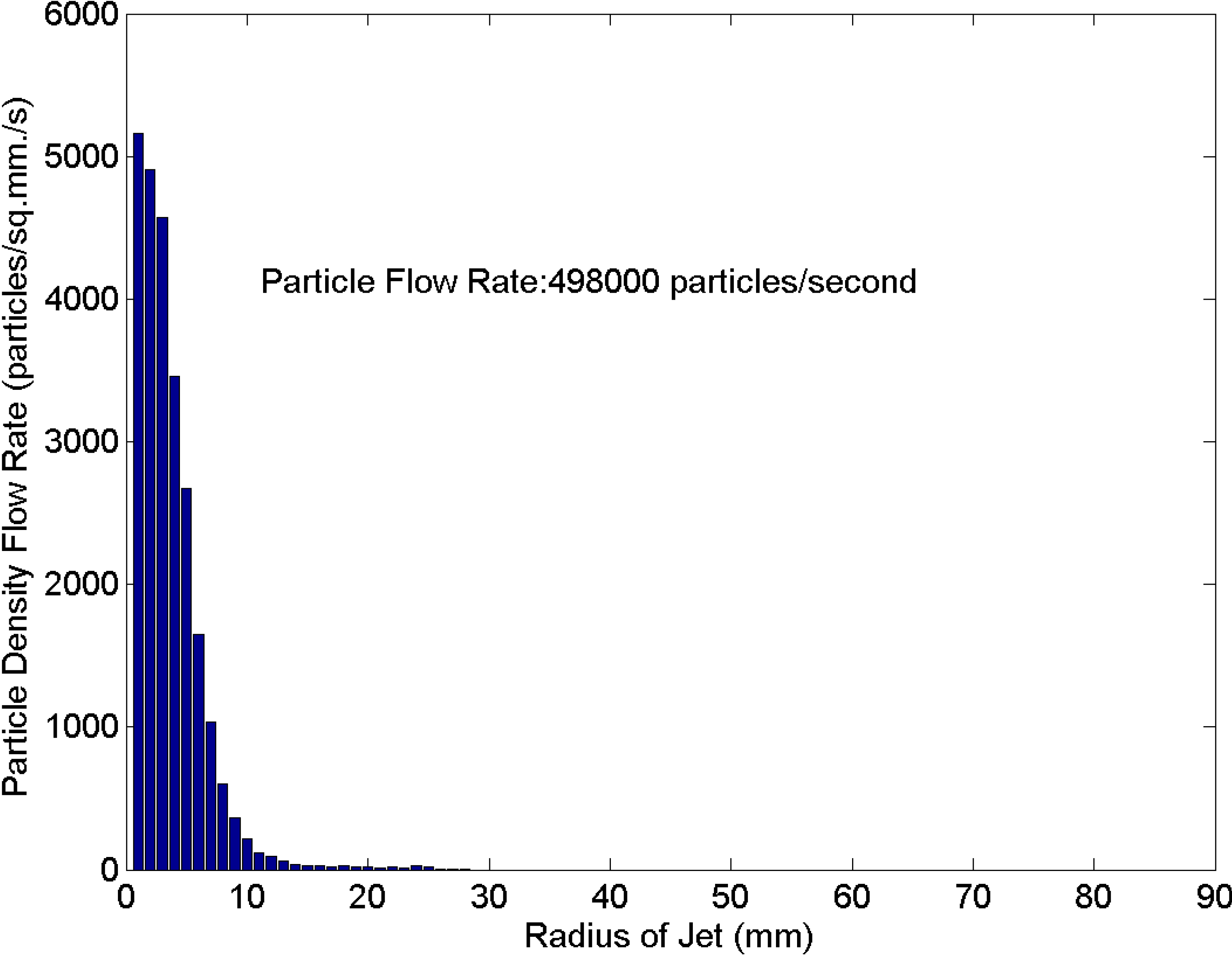
Figure 17. Experiment 2: Radial particle distribution at 10 cm from origin of annular air jet. Exposure time: 200 μs.

Figure 17. Experiment 2: Radial particle distribution at 10 cm from origin of annular air jet. Exposure time: 200 μs.

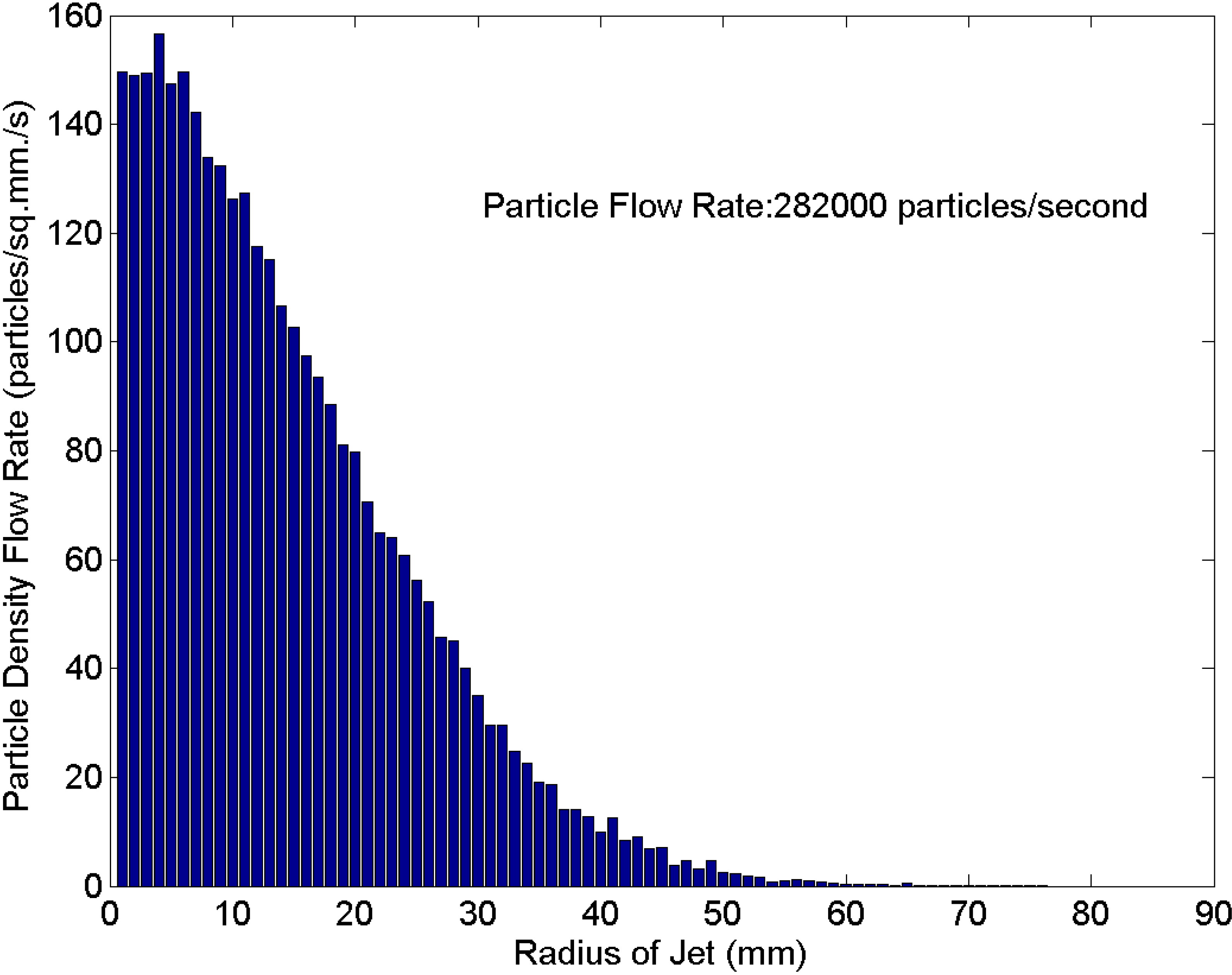
Figure 18. Experiment 2: Radial particle distribution at 20 cm from origin of annular air jet. Exposure time: 400 μs.

Figure 18. Experiment 2: Radial particle distribution at 20 cm from origin of annular air jet. Exposure time: 400 μs.

Figure 19. Experiment 2: Radial particle distribution at 40 cm from origin of annular air jet. Exposure time: 2 ms.

Figure 19. Experiment 2: Radial particle distribution at 40 cm from origin of annular air jet. Exposure time: 2 ms.

3. Numerical Work

Two phase flows were simulated using the finite volume based computational fluid dynamics (CFD) code Fluent. The two-phase flow model used here is an extension of the numerical work reported in a previous paper by Payne et al. [1]. The model used for two phase flow was the model found in the previous paper that agreed best with experimental results for the air only jets and had the coarsest mesh, ensuring the lowest computational cost. This model had a wedge shaped cross section with a 60° angle. The particle stream simulated assumed a particle flow rate of 10⁶ particles per second, about the top limit of the range of flow rates, a particle density of 800 kg/m³ and a weighted particle volume of 4.8 × 10⁻¹² m³ to give a particle mass flow rate of 3.8 × 10⁻³ kg/s. Since the model only spans one-sixth of the true domain circumferentially, this number was divided by 6. Figure 20a,b and Figure 21a,b show the averaged axial and radial velocities of the particles at 10 cm and 20 cm from the origin of the annular air jet respectively. These results are compared with the experimental results in Figure 22a–d, shown in the Discussion.

Figure 20. Experiment 1: Numerical simulation of two phase flow. The particle (a) axial and (b) radial velocities at 10 cm from the origin of the annular air jet averaged over 1 mm radial increments.

Figure 20. Experiment 1: Numerical simulation of two phase flow. The particle (a) axial and (b) radial velocities at 10 cm from the origin of the annular air jet averaged over 1 mm radial increments.

Figure 21. Experiment 1: Numerical simulation of two phase flow. The particle (a) axial and (b) radial velocities at 20 cm from the origin of the annular air jet averaged over 1 mm radial increments.

Figure 21. Experiment 1: Numerical simulation of two phase flow. The particle (a) axial and (b) radial velocities at 20 cm from the origin of the annular air jet averaged over 1 mm radial increments.

4. Discussion

Payne et al. [1] show Gun Head 2 has been effective in eliminating the recirculation zone at the exit of the powder air jet, at least over the annular air jet to central air jet velocity ratios used in this work. Figure 6a shows that most of the particles flow around the recirculation zone created by Gun Head 1, the original design, thereby increasing the radius of the particle stream. This radius decreases immediately downstream of the recirculation zone due to the influence of the annular air jet. The dual maxima shape of the first curve in Figure 8b indicates the impact of the recirculation zone on the particle distribution right at the exit, whereby most of the particle stream is pushed towards the nozzle edges, leaving the valley in the distribution curve around the flow axis. No such deformity exists in the first curve shown in Figure 8a, for Gun Head 2, as evidenced by the single peak distributions right from the start. Similarly, no double peak distributions are observed in similar plots from Experiments 1 and 3, not shown here.

Figure 6b together with Figure 7a,c,e show that the small inward radial velocity component of the annular jet created by Gun Head 2 in the near field, provides all particles with a small inward radial velocity that concentrates the particle stream into a smaller radius beginning at the tip of the central nozzle. Figure 8a and Figure 9a shows this effect of Gun Head 2 extends downstream. The radius of the particle stream created by Gun Head 2 is always smaller than that created by Gun Head 1. This feature of Gun Head 2 shows it is an improvement over Gun Head 1 because it ensures that all particles would flow through the same, or almost the same, part of the flame and would be heated to similar temperatures. When the particles are at similar temperatures, they will have similar physical properties ensuring a more uniform coating.

Figure 9a,b also compare the data gathered for this paper with the data of Mostafa et al. [5], Fan et al. [11] and Birzer et al. [12] by superimposing the half-maximum particle stream boundaries from these three references on both graphs. In case of the Gun Head 2, Figure 9a, they are shifted downstream by 14 mm, to match the particle release point. The data of Birzer et al. [12] and Fan et al. [11] match the particle spread rate reasonably well for the Gun Head 2 case. The data of Mostafa et al. [5] stands out both from the data gathered for this paper and from these two other data sets. Fan et al. [11] used Laser Doppler Anemometry to detect particle concentrations, Birzer et al. [12] used light nephelometry and Mostafa et al. [5] used Phase Doppler Anemometry. In all three literature sources, the velocity ratio was around 1.5 with the annular jet faster than the central jet. Our velocity ratios were much higher, as indicated approximately in Table 3. Farther from the nozzle, starting at about z = 80 mm, the particle spread rate for Gun Head 2 becomes linear, indicating a transition towards self-similarity. The same trend is seen in the data from Fan et al. [11] and Birzer et al. [12], with a similar spread rate.

The axial velocities of the particles shown in Figure 12a illustrate the momentum coupling by drag that occurred in the two phase jet in its near field, when the faster annular air mixed with the air from the central jet and accelerated the slower particles. It is expected that at larger axial distances where the particle axial velocities are larger than the air axial velocities the momentum coupling would be reversed. Some of the axial momentum of the particles would be transferred to the air, again through drag resulting in two way momentum coupling.

The Stokes number calculated for this inert two phase jet, an average of 120, suggests the turbulent vortices have little effect on the particle motion. The straight lines the particles travel confirm this prediction. However, the influence of turbulent vortices cannot be ruled out entirely, since particles experience a wide range of Stokes numbers due to their wide size variation and variations in the flow field over the length studied. Kennedy and Moody [18] made a quantitative study of variations in the Stokes number used here, for a two phase jet without any particle size variation. They found it varied by about an order of magnitude over the flow field.

An important distinction must be made between the time varying component of the fluid velocity and the time averaged component of the fluid velocity. While the time varying component of the fluid velocity had little or no effect on the particle velocities in this work, the time averaged component of the fluid velocity, in particular the velocity of the annular air jet, accelerated the particles in the near field. Again, it is expected that in the far field, the air and particles would again exchange axial momentum on a time averaged basis, but with the particles as the source and the air as the recipient.

Figure 17, Figure 18 and Figure 19 show the radial variation in particle flow rate per unit area per second for Experiment 2 at three distances from the gun head obtained from the cross sectional images. These distributions show the spreading of the particle stream with increasing distance from the gun head. If the half-maximum value is used as an indicator of jet radius, the corresponding radii in Figure 17, Figure 18 and Figure 19 are approximately 5 mm, 10 mm, and 20 mm, for z distances of 100 mm, 200 mm, and 400 mm, respectively. The particle stream radii at half peak from Figure 9a, based on analyzing the longitudinal images, are approximately 4 mm and 9 mm for z = 100 mm and z = 200 mm, respectively. The agreement between the particle stream radii found from the cross sectional images and the longitudinal images is satisfactory, especially given that these two estimates are obtained using two very different sets of data gathered at different times and analyzed differently. The wide variation in total particle flow rate per second is a result of the equally wide variation in the rate at which the ground polymer particles are added to the air in the line feeding the central jet.

Figure 17, Figure 18 and Figure 19 also shows the radial distribution of the particle density is roughly Gaussian although the particle flow rate per unit area never decreases to zero smoothly. Further statistical analysis was performed on the particle distributions in the cross sectional images to try to determine whether the particle distribution changed with total particle flow rate. The results of this work were not satisfactory. Consequently, more work is required to answer this question.

Each of the three histograms of the particle distributions at 100 mm from the cap face has a tail extending to an unexpectedly large radius. This maximum radius decreases as the momentum of the annular air jet increases from Experiment 1 through Experiment 2 to Experiment 3. The cause of this tail is not known and needs to be found in future work.

Comparison of the results shown here with Mostafa et al. [5], Fan et al. [10,11], and Birzer et al. [12] revealed that all four bodies of work show that the particle distribution as a function of radius is always roughly Gaussian, with the maximum particle concentration on the centerline of the jet. The commonality of these two features in the case of a free coaxial jet, a confined coaxial jet, and a coaxial jet exiting into a co-flowing stream show that qualitatively these differences have no effect on the particle distribution. However, it is also essential to realize that these differences will have a quantitative effect on the particle distribution, along with particle density, particle size distribution, and particle shape.

Analysis of the photos of the longitudinal sections found substantially the same results for all three experiments so only the analysis of Experiment 3 is discussed. Figure 12, Figure 13 and Figure 14 show that there is a wide range in particle axial velocities at any particular distance from the gun head, although the overall trend is for the axial velocities to drop as distance from the gun head increases, as expected. The lower particle density at the largest radii causes an increase in the length of the error bars for this area.

The radial velocities shown in Figure 12, Figure 13 and Figure 14 exhibit an interesting trend. In all cases the plot of radial velocity vs y value forms a band diagonally across the graph, although at z = 100 mm the radial velocities increase, roughly level off, and then increase again, all with increasing distance from the jet centerline. This velocity trend is not present in the same plots of the radial velocities at z = 100 mm created by analyzing the images of particles in Experiments 1 and 2. The increase in radial velocities followed by a rough levelling off and then an increase could be connected with the mixing of the two jets. This result needs to be studied further and shows similarity to some results of Nijdam et al. [19] who studied inert droplets from a central air jet mixing with coflowing air. At z = 200 mm and z = 400 mm the radial velocities more closely follow the expected trend. They are negative on one side of the centerline of the particle stream and positive on the other. This result agrees qualitatively with the cross sectional results, where it is observed that the radius of the particle distribution at successive downstream cross sections increases. This increase is only possible if the radial velocities on opposite sides of the center of the particle stream are opposite. The radial velocity was also found to increase with y value. The particles with the faster radial velocities will travel further in any set amount of time.

Fan et al. [10,11] found the smaller particles were moved to greater radii faster because of their reduced mass and thus the smaller particles were at the outside of the particle stream in a confined jet, with the larger particles at its center. The same pattern is probably present here, although without measurements of the particle size, there is no way to verify it.

Figure 22a–d compare the experimental and numerical values of the particle velocities at z = 100 mm and 200 mm. The magnitude of the velocities from both types of data agree reasonably well. This agreement is surprising because the particle flow rate and the particle size distribution used in the numerical model were thought to be an absolute maximum and a rough estimate of their respective true values. However, comparison of the maximum radius of the particle distribution between the numerical simulation and experiment shows that the numerical work dramatically underestimates this radius, especially at z = 100 mm.

Figure 22. Experiment 1: Comparison of the experimental and numerical values of the particle (a,c) axial and (b,d) radial velocities at (a,b) z = 100 mm and (c,d) z = 200 mm.

Figure 22. Experiment 1: Comparison of the experimental and numerical values of the particle (a,c) axial and (b,d) radial velocities at (a,b) z = 100 mm and (c,d) z = 200 mm.

In addition to these analyses, an effort was made to determine where the minimum radius of particle distribution occurred and at what distance from the cap face. The results obtained from the longitudinal section photos were not meaningful in this case. The tapering off of the radial distributions shown in Figure 17, Figure 18 and Figure 19 occurs over the entire length of the particle stream, making it difficult to find a satisfactory criterion to determine the stream boundary.

5. Conclusions

The new nozzle design clearly offers advantages over the previous design. The near field photos show that the recirculation zone has been eliminated for the same mass flow rates from the central and annular jets. The new design also produces a much narrower radial distribution in the near field, especially at the two higher momentum ratios. Comparisons of particle distribution widths based on the analysis of longitudinal and cross-sectional images show satisfactory agreement and give confidence in the results obtained. Furthermore, particle velocity distributions obtained by numerical simulations agree satisfactorily with the data obtained by processing high speed camera images.

There are a number of opportunities for further work. The most important topic is to understand fully how the radial velocity of the annular air jet alters the mixing of the two jets and whether the particles, in turn, have a significant effect on this mixing. It is also very important to measure the axial and radial velocities of the air to better understand the exchange of momentum between the two phases. The cause of the tails in the histograms, particularly at 100 mm from the cap face, needs to be found. Further improvements in experimental, and especially in numerical methods are needed to address the influence of irregular particle shape on the results. To that end, experiments with spherical particles could provide a valuable comparison, while a much larger effort in implementing irregular shaped particle movement in the numerical simulations would significantly improve the ability of numerical simulations to model real particle dynamics.