1. Introduction
Most of the wind turbines in Germany are located on flat terrain or in coastal regions. Alternatively, wind energy production in southern Germany, with its widely hilly or even mountainous and forested landscape, has become more and more attractive. However, finding appropriate sites with sufficient wind potential and an acceptable orography-induced turbulence level, especially in this densely populated territory, is a challenging task. Therefore, stable, practice-oriented, and validated computational fluid dynamics (CFD) models enabling the detailed prediction of wind flow in complex terrain for the micro-siting of wind turbines are desirable for enabling the reliable prediction of the wind speed, wind direction, and turbulence intensity. An overview over the possibilities for flow modelling for wind turbine micro-siting in complex terrain is given by Palma et al. [
1], where the need for nonlinear CFD models is highlighted.
One issue about the simulation of wind in complex terrain is the description of the anisotropic turbulence, which is driven by the inhomogeneous velocity distribution:
Another issue is that in forested areas, the model equations for momentum and turbulence have to be adjusted to get an adequate representation of additional drag forces as well as the generation and dissipation of turbulence. Two main approaches were developed and successfully applied in the past. One option is to introduce a roughness length z
0 in the logarithmic wall function [
10]. Another possibility is the use of canopy models, introducing source terms in the momentum and turbulence equations as first suggested by Svensson and Häggkvist [
11]. Similar approaches, all in combination with the standard k-ε model, have been adopted by Liu et al. [
12] and Green [
13]. Shaw and Schumann [
14] set up a test case of a homogeneous forested area, which commonly is used for the verification of these canopy models. Lopes et al. [
15] compared the different approaches using the data of Shaw and Schumann [
14] and devised a further canopy model. The use of a RSM for canopy flow was first described by Wilson and Shaw [
16]. Ayotte et al. [
17] established a model aiming at the simulation of neutrally stratified flow in heterogeneous landscapes and compared the simulation results with a flat terrain dataset. Ayotte et al. [
17] split the viscous dissipation into a contribution of the spectral eddy cascade, as well as a foliage contribution and the implementation of the RSM is based on the transport equation for the dissipation of the turbulence kinetic energy of the spectral eddy cascade. Dimitris and Panayotis [
18] used a similar approach to Ayotte et al. [
17]. However, the contribution of the vegetation is considered as source term directly in the transport equation for the total dissipation of turbulent kinetic energy. Dimitris and Panayotis [
18] compared the simulation results with measurements from laboratory channels with aquatic vegetation. An application of these kinds of RSM capturing canopy effects for the micro-siting in complex terrain is not known to the authors, indicating that there is a strong need for validation.
In the following study, we describe a way to carry out flow modelling in complex, forested terrain that is accurate and fast enough for micro-siting and for planning of measurement campaigns. The turbulence model is one of the key factors to get an accurate prediction of the wind velocity and the turbulence intensity, which are the essential measures for the power generation and fatigue load of wind turbines. For this, the standard k-ε, RNG k-ε, and Reynolds stress turbulence models are compared. Additionally, canopy models for the description of forestry in the momentum equation and turbulence models are implemented to capture additional drag force as well as production and dissipation of turbulence. The problem of finding realistic boundary conditions for the simulation of wind fields in complex terrain is tackled using data from the weather model COSMO-DE of the German Meteorological Service (DWD) [
19]. The models are verified for the homogeneous canopy test cases from Shaw and Schumann [
14]. The validation of the models is carried out by means of an unmanned aerial vehicle (UAV) and 3D-ultrasonic anemometer measurement data for the WindForS test site.
2. Computational Model
The computational method is implemented in the commercial software ANSYS CFX Version 17.0 [
20], based on the finite volume approach. The momentum equation in an inelastic formulation and the energy equation are solved. Turbulence is either described by the standard k-ε model, the RNG k-ε models, or the Reynolds stresses model. The pressure-weighted interpolation method (PWIN) [
21] is used to prevent the decoupling of velocities and pressure on the non-staggered grid. The convective fluxes are approximated for all transport equations with a bounded second-order upwind scheme.
Additional source terms are implemented to incorporate stratification of the Earth’s atmosphere and Coriolis force in the momentum equation. Furthermore, the capabilities of the software are extended to capture the influence of different land use on drag forces, as well as turbulence production and dissipation. The computational model is described in more detail in the following section.
2.1. Continuity and Momentum Equation
Fluid flow is described in a formulation of the continuity and momentum equations using the Boussinesq approximation [
22], where density is only influenced by buoyancy forces.
Momentum equation:
Θ is the potential temperature and
is the average perturbation of pressure to the hydrostatic reference state defined according as follows [
23]:
with β = 42 K, T
0 = 288.15 K, p
0 = 100,000 Pa, R
d = 287.05 J/(kg K), and g = 9.81 m/s
2.
The forest canopy can be modelled as a porous media by means of an additional drag force F
W,i in the momentum equation (Equation (2)):
where a is the local foliage density in the dependency of forestry height, C
D is the constant drag coefficient set to 0.30, and |u| is the magnitude of the velocity vector.
The Coriolis force terms F
C,i in Equation (2) are defined as follows:
with the average latitude ϕ depending on the area under consideration and the angular velocity of the earth Ω = 7.292 × 10
−5 s
−1.
The effective viscosity is a combination of the molecular viscosity μ and turbulent viscosity μ
t:
μ
t can be expressed by the turbulent kinetic energy k and the dissipation of the turbulent kinetic energy ε assuming isotropic turbulence:
2.2. Energy Equation
Energy transport is described by means of the potential temperature Θ:
with the turbulent Prandtl number
set to 1.0.
2.3. Two Equation Turbulence Models
Two equation turbulence models are commonly used for industrial applications because of their numerical stability and low demand on computer resources. In this study, the standard k-ε model and the RNG k-ε model are applied for the simulation of wind flow in complex terrain, solving transport equations for the turbulent kinetic energy k and the dissipation of turbulent kinetic energy ε.
2.3.1. Standard k-ε Turbulence Model
The turbulent kinetic energy k and dissipation of turbulent kinetic energy ε are described with the following transport equations:
The turbulence production due to turbulent eddy viscosity is calculated as follows:
The constants of Equations (10)–(12) are summarized in
Table 1 and are chosen according to Launder and Spalding [
24].
2.3.2. RNG k-ε Turbulence Model
The RNG k-ε model of Yakhot et al. [
25] includes a correction to the k-ε model by revaluating the constants. No adjustment of the constants is made, they are derived analytically from the RNG theory (renormalization group methods). Equations (10) and (13), as well as Equations (11) and (14), are identical except for the constants:
The constants used for the RNG k-ε turbulence model are summarized in
Table 2.
2.3.3. Canopy Model Source Terms for Two Equation Turbulence Models
Additionally, terms for production and dissipation have to be added to the transport equations for turbulent kinetic energy (Equations (10) and (13), respectively) and dissipation of turbulent kinetic energy (Equations (11) and (14), respectively). Generally, these source terms are written according to Katul et al. [
26]:
In this study, the model of Liu et al. [
12] is chosen, taking the dissipation and production terms with the constants summarized in
Table 3 into consideration.
2.4. A Second-Order Turbulence Closure
The turbulence model is based on the formulation of Launder et al. [
27] and its extension on vegetated canopy flows of Ayotte et al. [
17] in combination with those of Dimitris and Panayotis [
18].
Reynolds Stress Turbulence Model (RSM)
In case of the Reynolds stress model, six transport equations have to be solved for the computation of the Reynolds stress tensor:
where P
ij is the production term:
The pressure–strain correlations Φ
ij,1 and Φ
ij,2 are described according to Rotta [
28] and Launder et al. [
27], respectively:
With
and
and
are additional dissipation and production terms capturing the increase of dissipation and production within the canopy [
17].
Note the positive sign for the additional dissipation terms and the factor ½ in Equation (26) [
29].
The turbulent kinetic energy k is computed explicitly from the normal Reynolds stresses:
The implementation of the Reynolds stress model is based on the transport equation for the turbulence eddy dissipation ε, mainly for the purpose of numerical stability. Dimitris and Panayotis [
18] suggested the following formulation using a transport equation for the total turbulence eddy dissipation including an additional source term
for the canopy:
In the canopy source term,
the internal time scale in the canopy according to Uittenbogaard [
30] is included:
Depending on the distance between the stems and their diameter, the length scale of the turbulent eddies is reduced in the canopy, decreasing their lifetime. For this reason, the internal canopy time scale
based on the total time scale
may be adapted using a multiplication coefficient
to fit the model results to measurements, as discussed in Lopez and Garcia [
31].
All model constants used for the Reynolds stress model are summarized in
Table 4.
3. Model Verification Using a Homogeneous Canopy Test Case
The different turbulence models, including their extension for the description of flow within the canopy, are verified via the test case of Shaw & Schumann [
14] representing flat terrain and constant canopy height of h = 20 m. The test case enables the comparison of different turbulence models in combination with the canopy models independently of the influence of the orography due to the homogeneous landscape. The computational domain has an extent of 9.6 h × 4.8 h × 3.0 h, spatially resolved with 96 × 48 × 30 grid lines in
x-,
y-, and
z-directions in the original mesh. Additionally, a refined mesh with 192 × 96 × 120 grid lines is set up to increase the spatial resolution by a factor of two in the
x- and
y-directions, and by a factor of four in the
z-direction. The flow is aligned along the
x-axis, with the
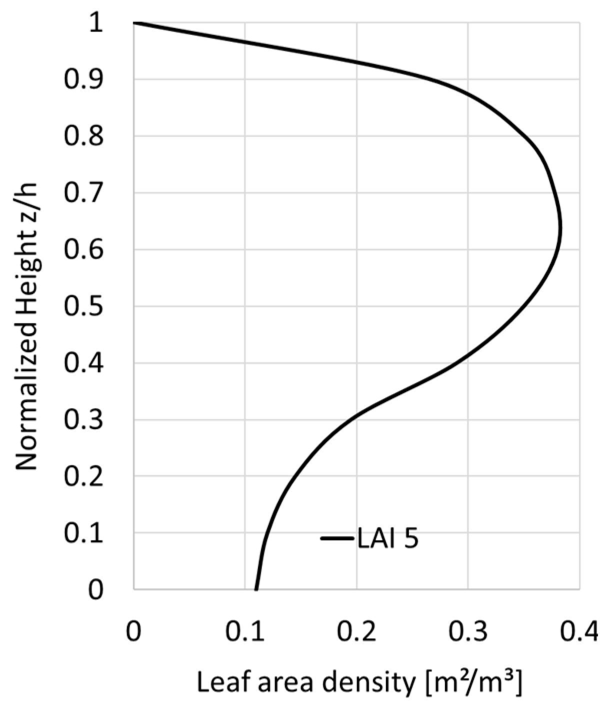
z-axis pointing upwards in the vertical direction. For the lateral and longitudinal boundaries, periodic boundary conditions are used. In the case of longitudinal boundaries, a pressure gradient along the test case is prescribed to reach an average axial velocity of 2 m/s. The leaf area index (LAI) can be computed with Equation (32) from the local leaf area density
shown in
Figure 1.
LAI was set to five, which is an appropriate choice for a coniferous forest and deciduous forest in summer [
14].
The distribution of the heat source was neglected, representing a neutral stratification of the atmosphere for the verification of the canopy models according to Lopes et al. [
15]. Despite the reference solution of Shaw and Schumann [
14] referring to a weakly unstable stratification, the comparison of the different canopy models seems to be appropriate when assuming a minor influence of the stratification on the flow in this test case with limited height.
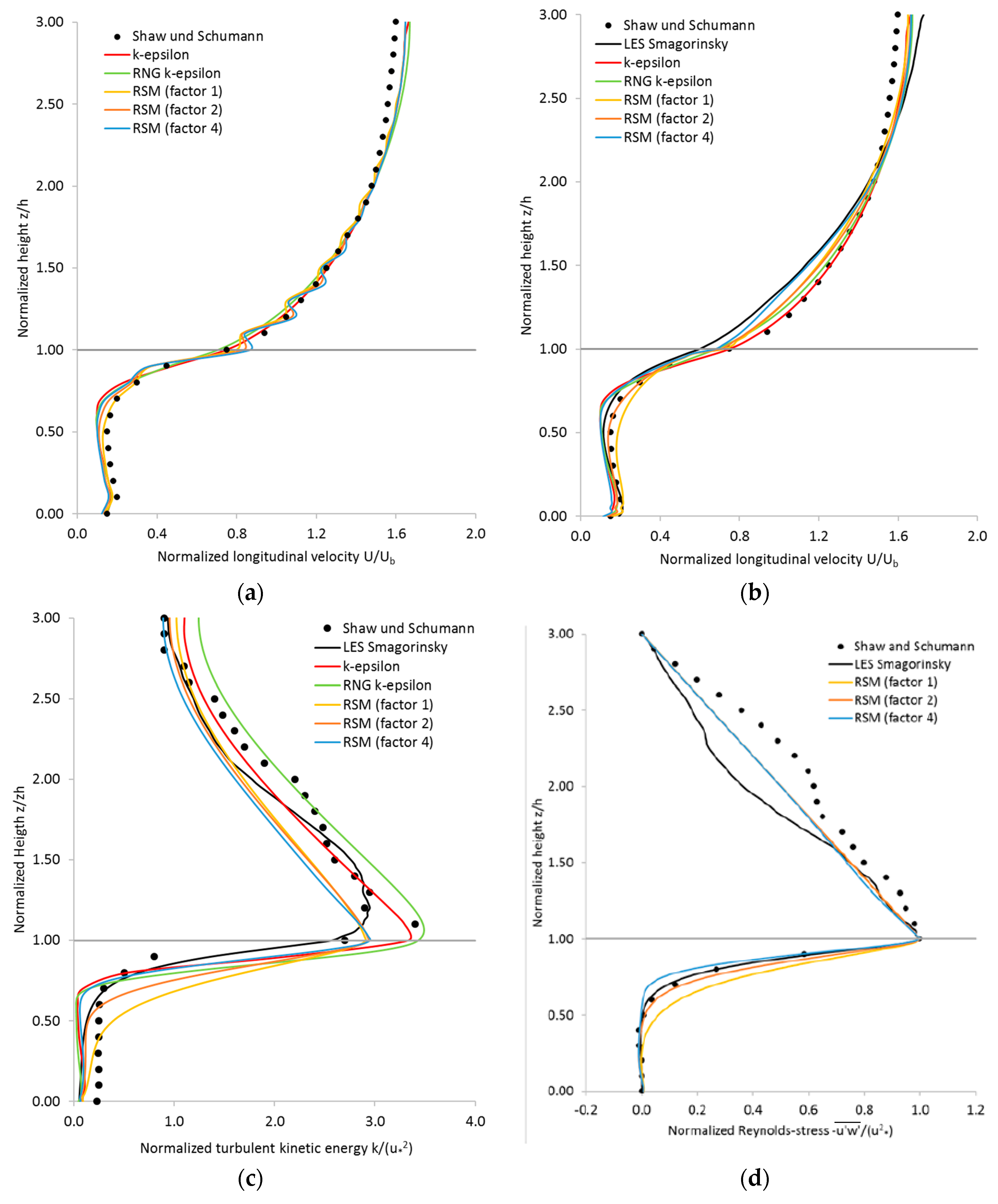
In
Figure 2a, the profiles of the normalized longitudinal velocity are plotted versus the height for the standard k-ε, the RNG k-ε, and the Reynolds stress model, as well as for the LES reference solution of Shaw and Schumann [
14]. For the RSM, the factor
of Equation (31) describing the turbulent time scale in the canopy is varied to get a more accurate fit with the reference solution. The velocity u is normalized by the vertically averaged longitudinal velocity. All turbulence models investigated can capture the maximum of the wind speed at a height of z/h ≈ 0.1 and the minimum of the wind speed at a height of z/h ≈ 0.5. Wiggles are observed for the RSM velocity profiles above the forest. This effect is the result of mesh resolution, which is too coarse in the
z-direction. For this reason, the RANS simulations are rerun on the refined mesh and the results are depicted in
Figure 2b–d. Additionally, a LES simulation with the Smagorinsky subgrid-scale model is set up to get a conformal comparison based on an identical mesh resolution for all models. On the refined mesh, smooth curves for the normalized velocities are obtained for the RSM (
Figure 2b). However, the differences for the turbulent models become larger in and above the canopy than for the original mesh. It can be stated for the RSM that the velocities are getting smaller in and just above the canopy, but larger in the free flow by increasing factor
for the internal time scale from 1 to 4. An excellent agreement between the LES and RSM is reached by using a factor
.
The spread of the turbulent kinetic energy normalized with the friction velocity
(
Figure 2c) is larger than the spread of velocity within the canopy. The gradient of normalized kinetic energy becomes very high around z/h ≈ 0.7 in case of the RSM with the factor
, as well as for the standard k-ε and RNG k-ε models. For smaller factors (
), for the RSM as well as for the LES, the increase of the normalized turbulent kinetic energy over the height of the canopy is smaller. Looking at the maximum of the normalized kinetic energy above tree top, the values are over-predicted by the standard k-ε and RNG k-ε models. For the RSM, there is a good agreement with the LES solution independently of the factor
. However, this maximum is much broader for the LES than for the RSM.
Regarding the Reynolds stress
normalized by the Reynolds shear stress at the canopy top (
), the gradient towards the top of the canopy becomes larger with an increasing factor for the RSM model (
Figure 2d). The LES solution lies in between the RSM solutions using a factor
= 2 and 4 for the forested area.
To judge the agreement between the RSM with the LES reference solution quantitatively, the root mean square deviation (RMSD) values are computed for the forested area (
) as well as for the whole computational domain (
Table 5) regarding the normalized velocity, the normalized turbulent kinetic energy, and the normalized Reynolds stress. It is shown that for the evaluation of the whole domain, as well as particularly for the canopy area, the factor of 4 for the internal time scale in the canopy gives the lowest RMSD values for the three variables. It has to be considered that the diameters of the stems and the leaf area density vary with height of the forest, and therefore a constant factor
over height is a further approximation. However, this is an indication that the time scale of the eddy dissipation is increased in the canopy because of the smaller eddy length scales and that this effect can be captured by a scale factor
.
Generally, the results for the RSM fit very well using the factor with the LES reference and this setup is finally chosen for further simulations.
4. Model Setup for the WindForS Test Site
The computational domain includes the WindForS wind test site near Stötten (734 m a.s.l., 48.6654° latitude, 9.8655° longitude) in Baden-Württemberg, South Germany. In the past, various measuring campaigns using UAV (small unmanned research aircraft), sonic and cup anemometers, and Lidar were conducted to study the flow phenomena in complex terrain (Schulz et al. [
4]; Anger et al. [
32]; Hofsäß et al. [
33]; Wildmann et al. [
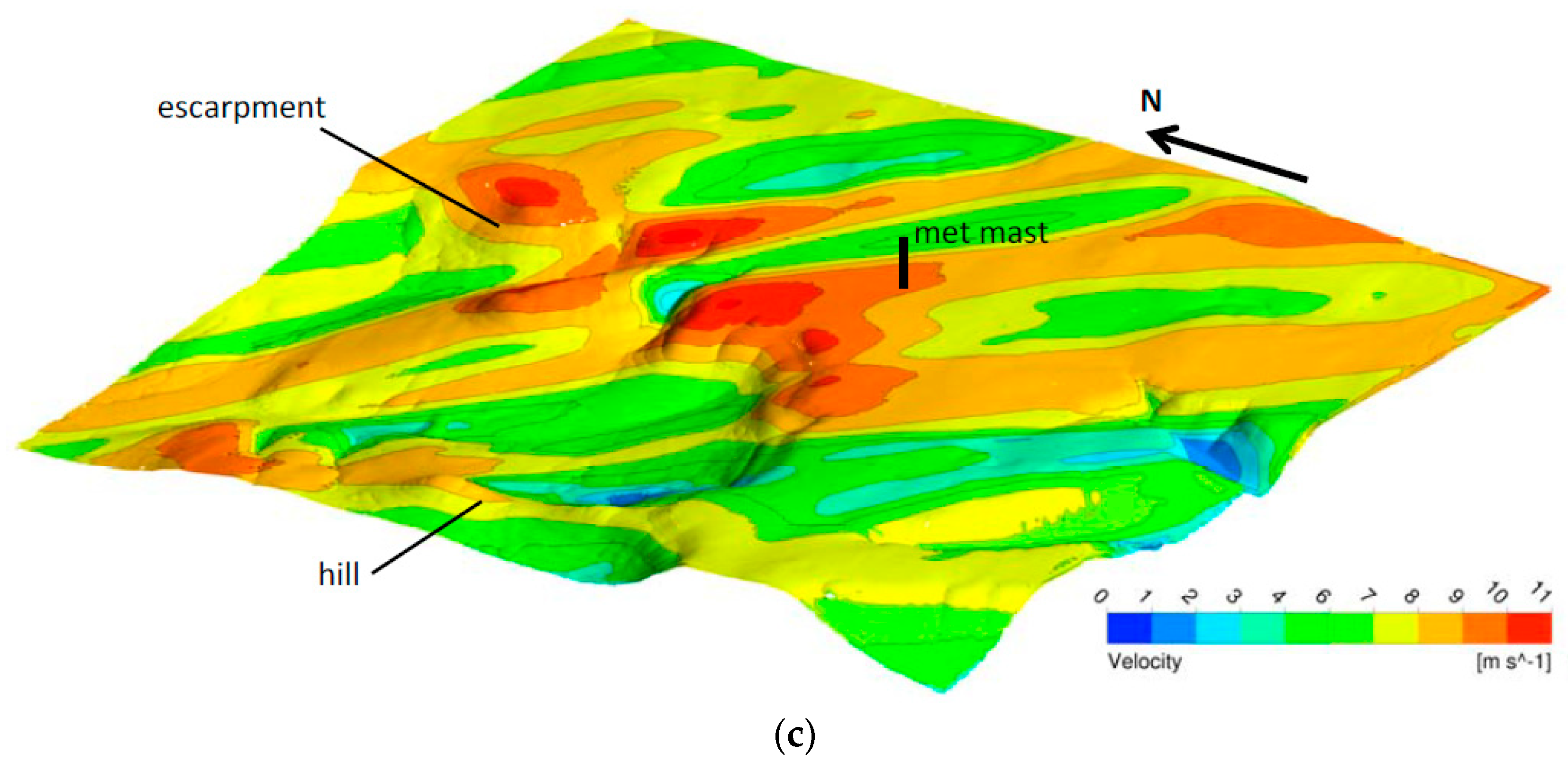
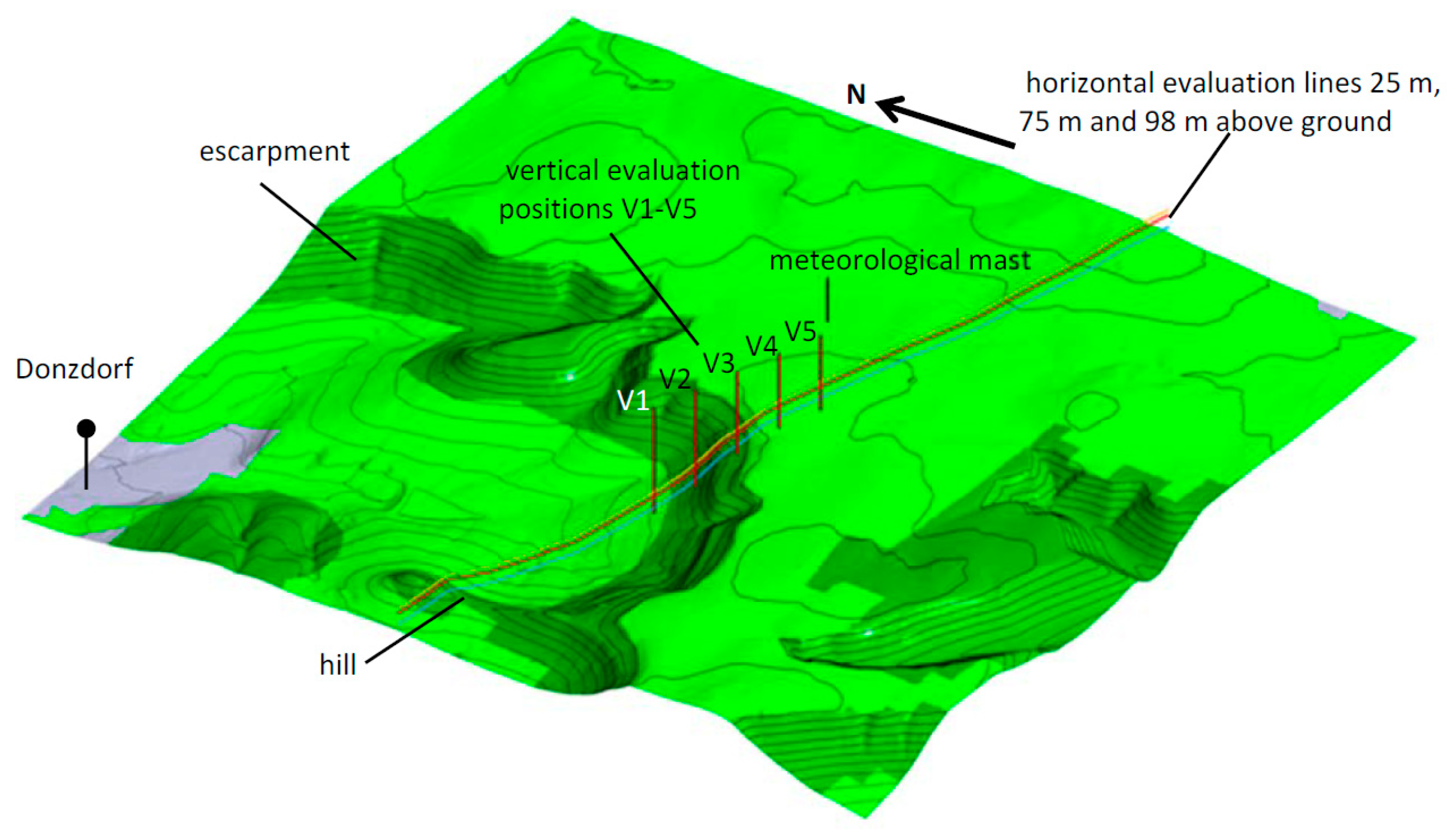
34]). The test site area is characterized by an escarpment located close to the towns of Geislingen an der Steige (464 m a.s.l.) and Donzdorf (407 m a.s.l.). The escarpment is completely forested, reaching a height of approximately 660 m a.s.l. at the upper ridge (
Figure 3).
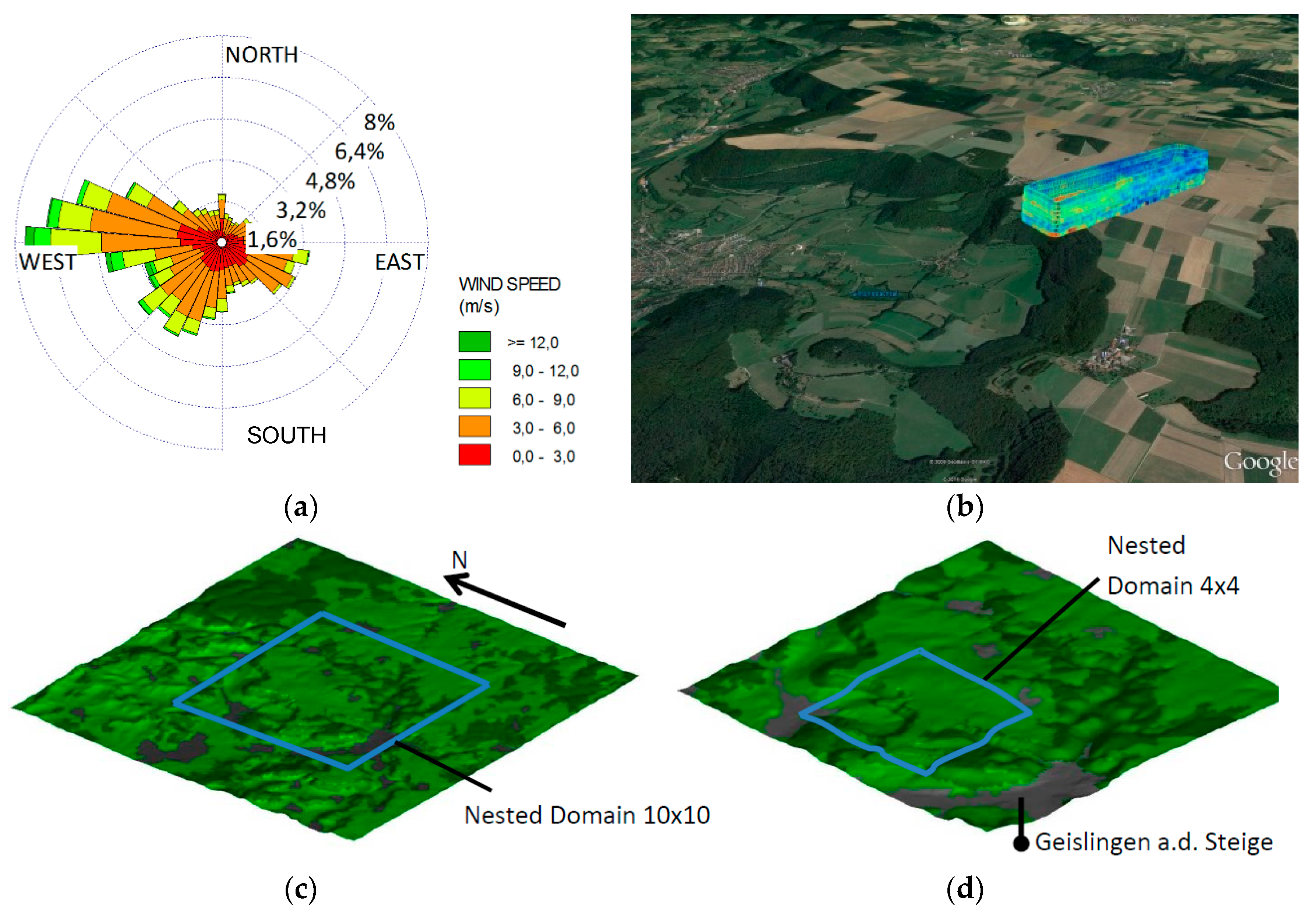
The main wind direction is north–west with an angle between 270° and 290°, as seen in the wind rose depicted in
Figure 4a. Generally, the flow domain features various hills and valleys, as well as forested and un-forested areas, making it an ideal test case for the use of numerical flow models in complex terrain.
Nested domains with varying size and resolution were used for the simulations of the test site. First, a computational domain of 20 km × 20 km × 2.0 km (parent domain) is chosen. From this, two nested domains with spatial extensions of 10 km × 10 km × 1.5 km (nested domain 10 × 10) and 4.0 km × 4.0 km × 1.5 km (nested domain 4 × 4) are chosen, reducing the horizontal extensions by a factor of around two. The spatial resolution and the number of cells are summarised in
Table 6.
The parent domain and the nested domain 10 × 10 were centred in the area of interest (
Figure 4c), whereas the nested domain 4 × 4 is shifted in a north–west direction to better capture the influence of the flow upstream depending on the flow direction (
Figure 4d). In
Figure 4c,d, the different land uses can also be seen (urban in grey, forest in dark green, agriculture in light green). All meshes are unstructured and mainly built of tetrahedral cells. On top of the ground, several prism layers are placed to get a constant spatial resolution in this area. For the nested domain 4 × 4, a resolution next to the ground of 1.0 m in the vertical direction and 10 m in the horizontal direction is reached. The nested domain 4 × 4 is depicted in
Figure 3 together with the measurement positons and the positions for the evaluation of simulation results.
The generation of the computational mesh, and therefore the reproduction of the Earth’s surface for the computational domain, is realized using the digital height model (DGM) and digitized landscape model (DLM) from State Authorities for Spatial Information and Rural Development Baden-Württemberg (LGL).
In case of the domain measuring 20 km × 20 km (parent model), weather data from DWD is used for the generation of boundary conditions. In particular, data from 27 March 2015 at 3:00 p.m. were selected, which are linked to the most frequently occurring north–west wind and dry, near-neutral conditions. Wind speed and wind direction are measured at the nearby DWD measuring station Stötten (734 m a.s.l., 48.6654° latitude, 9.8655° longitude) for this period of time showing a stable wind speed of around 7 m/s and a north–west wind direction of 290°.
The weather data is derived from the COSMO-DE weather model of DWD with a spatial resolution in the horizontal direction of approximately 2.8 km. Perpendicular to the Earth’s surface, a maximum vertical resolution of 20 m is reached close to the surface, rapidly increasing with the height above the surface. The weather data provides wind speed, pressure, density, air and surface temperature, as well as information about turbulence kinetic energy with a temporal resolution of one hour. Radiative heat transfer is neglected in the model.
The simulations were performed on a NEC LX-2400 cluster consisting of 180 blades equipped with Intel Nehalem Processors (2.27 GHz/2.80 GHz, 8 cores, 24 GB memory) and connected by an InfiBand network. The relative computational time per iteration on the nested domain 4 × 4 for the different turbulence models is summarized in
Table 7.
4.1. Initial Conditions for the Parent Domain
For lateral and top boundaries, data from the weather model is linearly interpolated to define the Dirichlet boundary conditions for velocities and temperature. At the top boundary, a flow in and out of the domain is allowed, whereas the flow for lateral boundaries is limited to one direction. No correction of the mass flow was needed, reaching a conservative one-way coupling of the COSMO-DE and CFD model.
4.2. Boundary Conditions for Nested Domains
For all cases based on nested domains with dimensions of 10 km × 10 km, as well as 4.0 km × 4.0 km, the boundary conditions are imposed using the solution provided by CFD simulation with the domain size of 20 km × 20 km and 10 km × 10 km, respectively. The boundary values for velocities, temperature, and turbulent quantities are interpolated according to the second order accurate discretization scheme on the boundary surfaces. For the nested domains, Dirichlet boundary conditions are defined for the lateral, top, and bottom boundaries. Again, for the top boundary, a flow in and out the domain is allowed.
4.3. Boundary Conditions at the Ground for Parent and Nested Domains
A wall model is used for the bottom boundary (ground) to handle velocities and turbulence quantities. Temperatures on the ground, which are extracted from the weather model data, are used as Dirichlet boundary conditions. For the different land use, displacement length z
0 is set to 0.02 m and 2.67 m for un-forested and urban areas, respectively. For the forested areas, a z
0 value of 0.02 m in combination with the canopy models is applied. An LAI of five representing deciduous forest with the LAD distribution according to
Figure 5 and a forest height of 20 m is used for the canopy model.
5. Results for the WindForS Test Site
In the following section, the results of simulations with the models described above for the test site Stötten are presented. They represent a general description of the wind flow on 27 March 2015 at 3:00 p.m., characterized by dry conditions and a thermally near-neutral stratification of the atmospheric boundary layer. The simulation results are compared with UAV and sonic anemometer measurements for the model validation.
5.1. Qualitative Comparison of Simulation Results
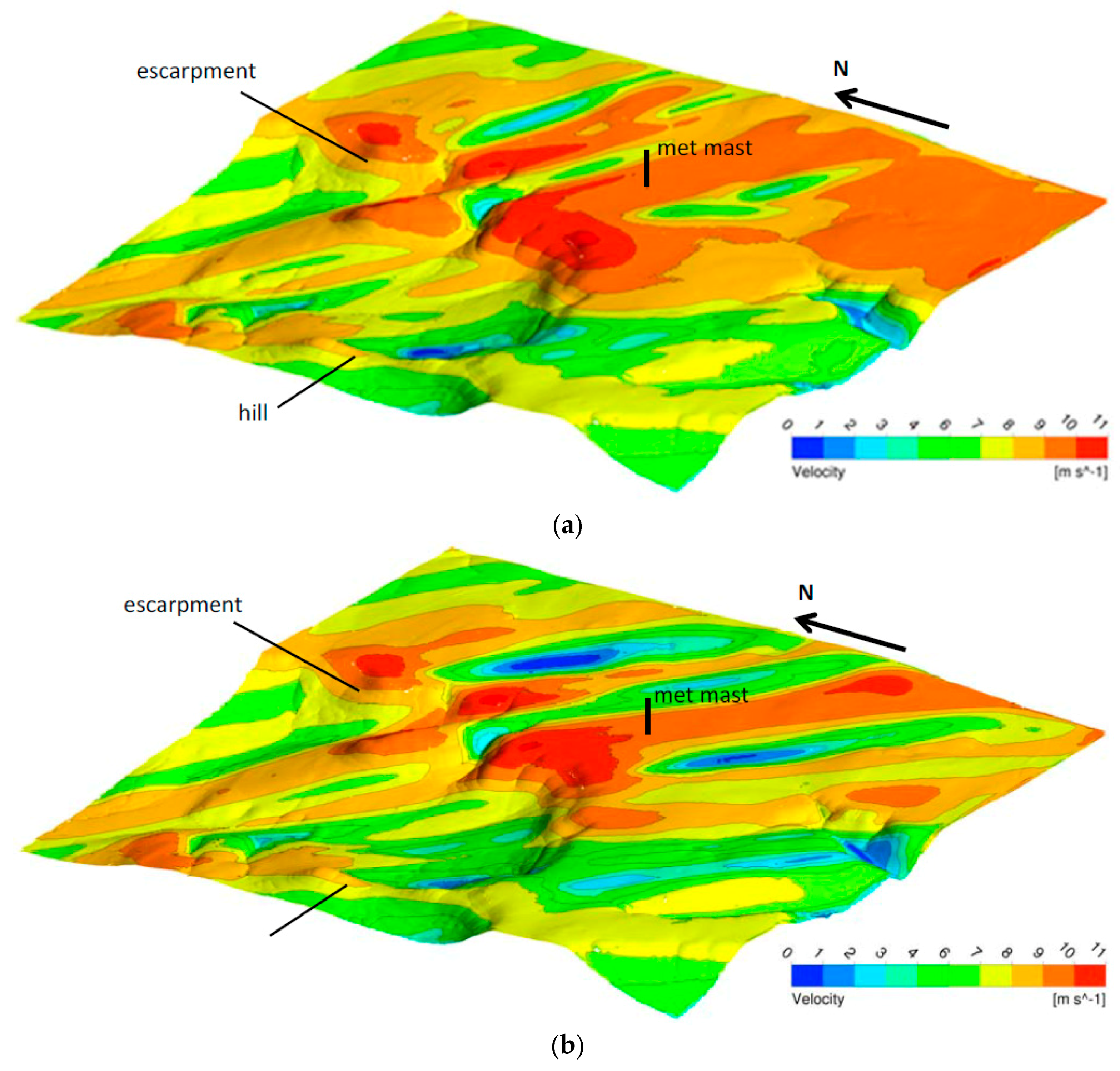
In
Figure 5a–c, the two-dimensional spatial velocity distribution at a constant height of 75 m normal to the Earth’s surface is depicted for the different turbulence models. For orientation, the position of the meterological mast as well as the escarpment and the hill are marked in
Figure 5a–c. A very heterogeneous flow along the surface becomes visible for all turbulence models characterized by a flow separation downstream the hill and a strong acceleration of the flow along the escarpment. Furthermore, downstream the crest of the escarpment streaks with reduced velocities are staggered with areas of accelerated flow. In the case of using the RNG k-ε model (
Figure 5b), this distribution is highly pronounced, whereas for the standard k-ε model (
Figure 5a), the flow is predicted almost equally. Generally, the computed velocities are higher on this level in the case of using the standard k-ε model than for the RNG k-ε model and the RSM (
Figure 5c). This becomes particularly obvious in the area, with downstream the hill and the escarpment showing the tendency of the standard k-ε model to under-predict flow separation zones. Looking at the main flow direction, it can be observed that the flow is directed more in easterly direction for the standard k-ε model than for the RNG k-ε model and the RSM model.
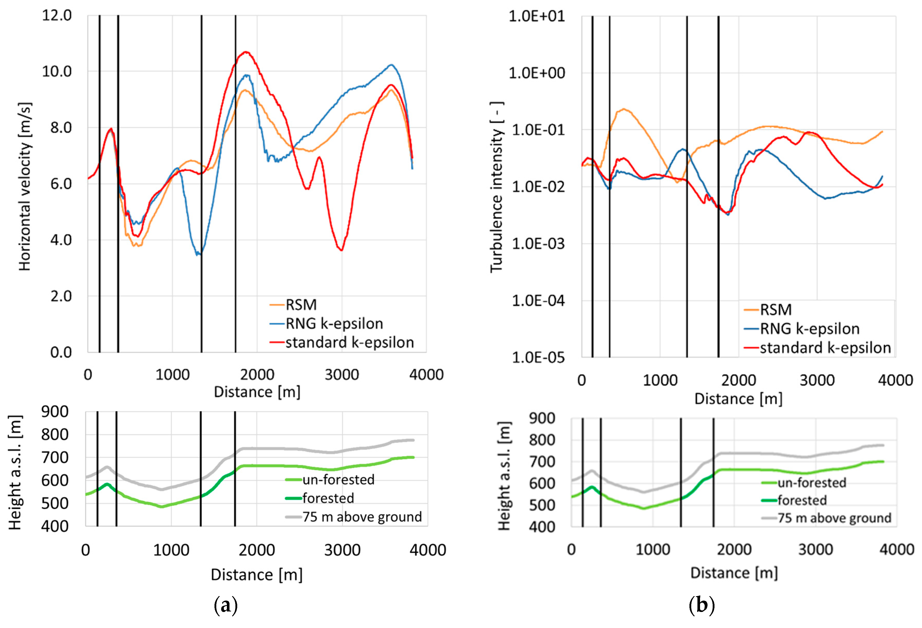
To get more detailed information, the results are contrasted in
Figure 6,
Figure 7,
Figure 8 and
Figure 9 along the evaluation lines shown in
Figure 3. The lines are located in a constant offset of 25 m, 75 m, and 98 m perpendicular to the Earth’s surface. The boundaries of the forested areas are marked in
Figure 6,
Figure 7,
Figure 8 and
Figure 9 with vertical black lines and the topography along the evaluation plane is depicted together with the evaluation line underneath the diagrams. In
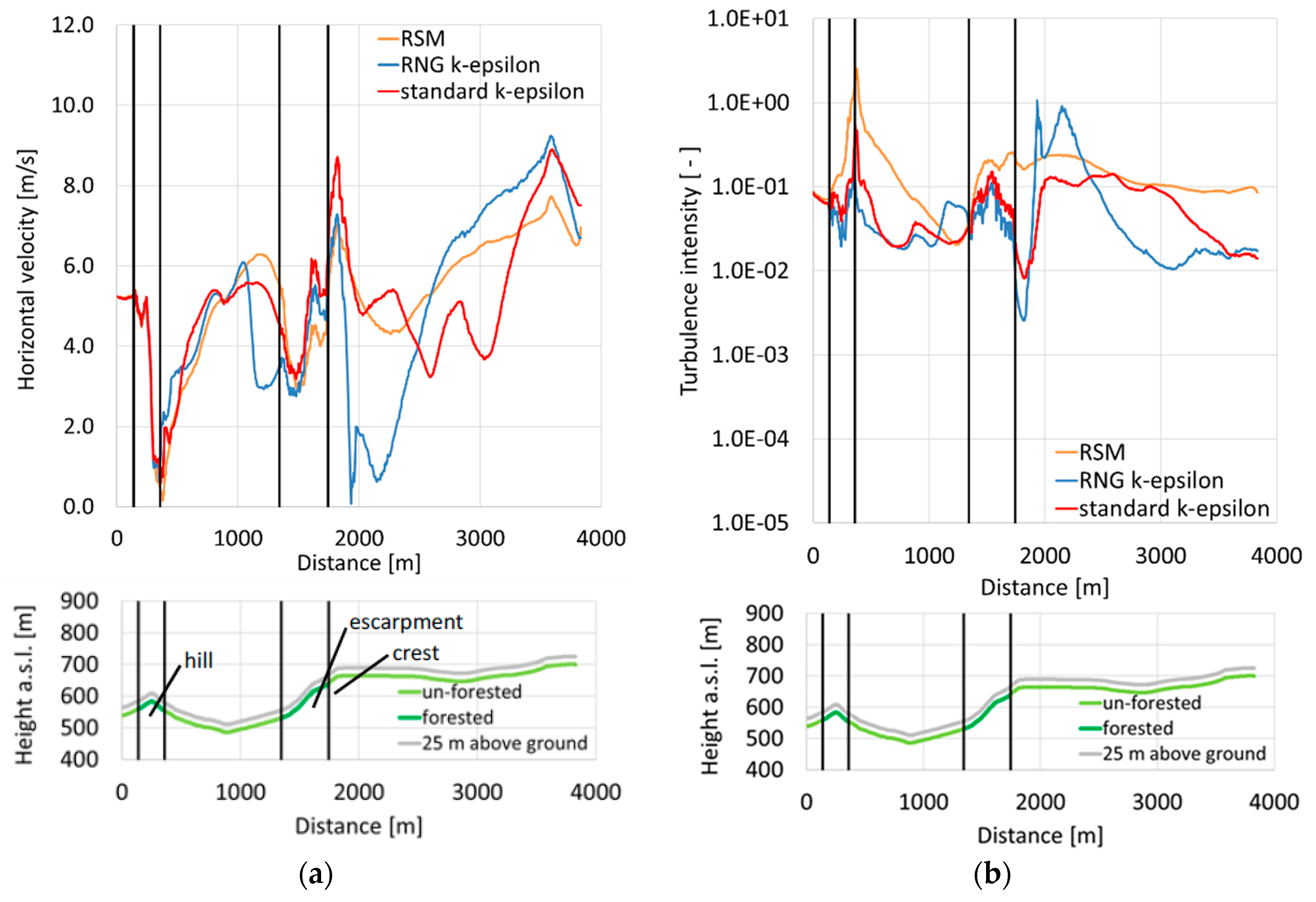
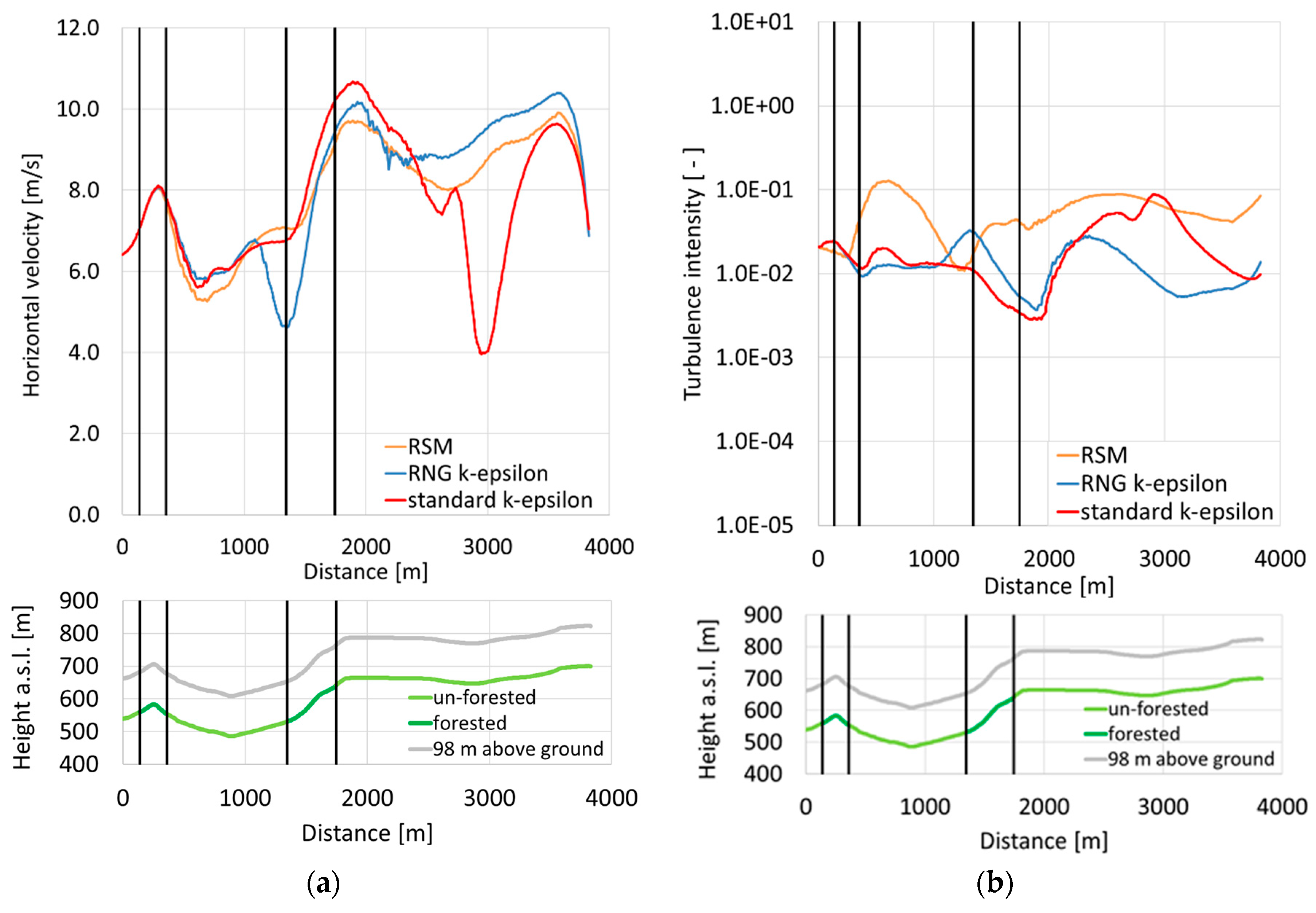
Figure 6a/b, the different turbulence models are compared for the 25 m distance above ground. Looking at horizontal velocity (
Figure 6a), only minor differences are found upstream the crest of the escarpment. The flow is decelerated downstream the hill and tends to separate. Subsequently, it is accelerated again along the escarpment reaching the highest velocity at the crest in the case of using the standard k-ε turbulence model. Downstream the forest edge at the crest, the results differ from each other. With the RNG k-ε model, a flow separation with reverse flow is predicted in this area, whereas for the standard k-ε model and the RSM, the flow is decelerated but still directed in the main flow direction. With increasing distance from the crest, the results predicted from the different turbulence models are increasingly converging. Considering the turbulence intensity (
Figure 6b), it is found that the increase is steeper upstream the hill as well as upstream the escarpment and it is decreasing much slower downstream for the RSM than in the case of the RNG k-ε and the standard k-ε models. This is an indication that turbulent kinetic energy is dissipated too rapidly in the case of the RNG k-ε and standard k-ε models.
Along the evaluation lines 75 m and 98 m above the ground, the flow accelerations due to the hill and the escarpment can still be seen in
Figure 7a and
Figure 8a, respectively. The two velocity maxima are on the same level for the two elevations. On both levels, the minima of the horizontal velocity between the hill and the escarpment, as well as downstream the crest, are visible accordingly. However, for the evaluation line 98 m, the deceleration of the flow is smaller than along the line at 75 m, indicating that the flow already becomes more equal in this higher elevation. Analogous to the line on 25 m, it can be observed that at the lines at 75 m and at 98 m (Figures 7b and 8b), the turbulence intensity is much stronger along the hill and along the escarpment, and that the decrease downstream to these obstacles is much lesser for the RSM than for the two equation turbulence models.
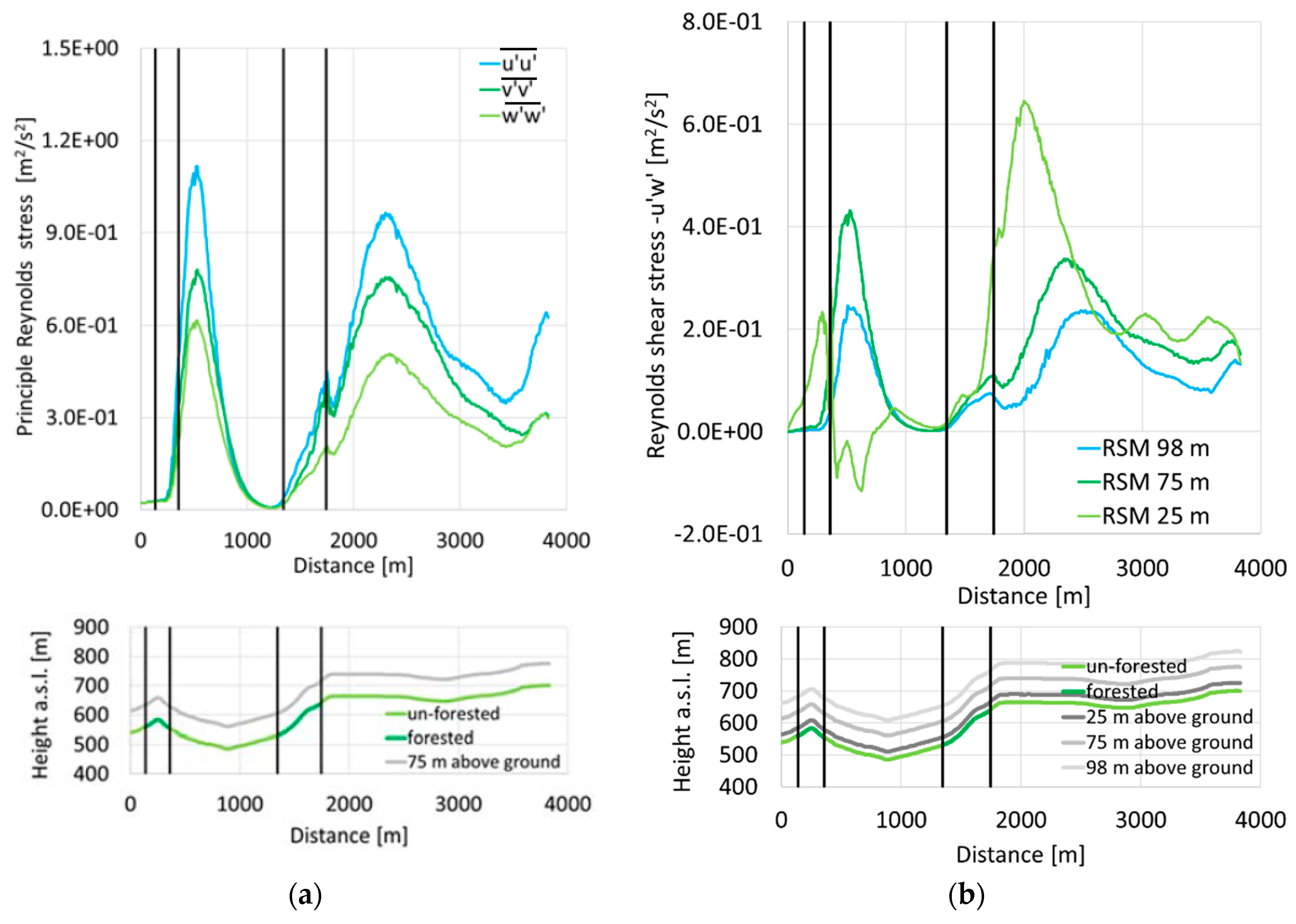
One major drawback of using the RNG k-ε and standard k-ε models for the simulation of wind flow in complex terrain is the assumption of an isotropic turbulence. To judge the differences of the Reynolds stresses in different directions, the principle Reynolds stresses computed with the RSM are depicted in
Figure 9a. Therefore, the Reynolds stress tensor is rotated in the main flow direction, which is aligned with the velocity component u. It can be seen that the principle Reynolds stresses differ up to a factor of two and that the anisotropy is driven as a result of the orography. Along the upwind side of the hill and the escarpment, the differences strongly increase and diminish at downwind sides. The Reynolds stress
directing in the main flow direction is always the biggest component, whereas the Reynolds stress
pointing in an upward direction is the smallest. Another interesting aspect for the wind energy production is the turbulent vertical momentum transport due to the shear stress
. In
Figure 9b, the shear stress
is evaluated at the levels 25 m, 75 m, and 98 m. Initially, at 25 m, the Reynolds shear stress is increased along the hill. As a result of the flow separation downstream the hill, the shear stress becomes negative, indicating turbulent momentum flow towards the Earth’s surface. The maxima of the Reynolds shear stress at the levels 75 m and 98 m due to the hill are slightly shifted in a downwind direction. Along the escarpment, the Reynolds shear stress is even more increased than along the hill. The maxima again are located just downstream the crest, with highest values for the lowest level at 25 m.
Figure 9b shows that along all evaluation lines, a constant shear layer is not reached.
5.2. Validation of the Model by Means of Measurement Data
In the following section, the different modelling approaches are validated against measurement data for the test site Stötten. Therefore, the results are compared with UAV measurements along vertical lines, particularly those placed at the escarpment within the computational domain. Additionally, sonic anemometer measurements from a meteorological mast are used.
5.2.1. Description of Measurements
Multipurpose Airborne Sensor Carrier (MASC)
MASC [
34] is a propeller-driven, unmanned single-electric-engine aerial vehicle (UAV) of 2.7- to 3.5-m wing span, developed and operated by the University of Tübingen. The total weight of the aircraft is 5 to 8 kg, including up to 1.5 kg of measuring devices. The typical horizontal flight speed of the UAV is 22 m/s airspeed, giving the optimum trade-off between high spatial resolution of measured data and gathering of atmospheric data from a certain area in a short period of time. MASC operates fully automatically except for landing and take-off. Height, flight path, and all other parameters of flight guidance are controlled by the research onboard computer system (ROCS). The overall endurance achieved with MASC is up to 90 min, which is associated with a flight distance of 135 km. MASC is standardly equipped with several subsystems specifically to measure the wind vector in three dimensions with a five-hole probe [
35], air temperature with fast fine-wire probes [
36], and humidity [
37] with a capacitive sensor. The measurement equipment is able to resolve wind and temperature fluctuations up to 30 Hz and humidity fluctuations up to 3 Hz, all sampled with a rate of 100 Hz. Additionally, an inertial measurement unit (IMU) and a global navigation satellite system (GNSS) provide position, altitude, and velocity of the aircraft above ground.
Three flights with a duration of one hour each were carried out on 27 March 2015 between 1:00 p.m. and 4:00 p.m. UTC. An example of a flight path is shown in
Figure 4b. Each flight is composed of several so-called racetracks, consisting of two legs (straight and level flight path) along the mean wind direction (west-east direction). Two racetracks were flown at each altitude. Legs where the UAV was flying into the wind were used for the analysis as this gives the lowest ground speed, and thus the greatest spatial resolution keeping the flight velocity with respect to the air constant at 22 m/s. This results in a varying ground speed, because the meteorological wind is fluctuating. On each and every leg, the wind velocity was arithmetically averaged over subsections of 20 m length (block averages). Each block comprises of an average time between 1.37 and 1.81 s depending on the wind speed, equivalent to 137 and 181 data points, respectively. The block means were subsequently averaged over all legs measured, that is, six racetracks at the same height. These values are depicted as black dots in
Figure 10a–e and
Figure 11a–e for the comparison of measurements with simulation results in
Section 5.2.2 representing a constant spatial resolution of 20 m.
Meteorological Mast
The meteorological mast is located approximately 1.3 km to the east of the escarpment (48.6658° latitude, 9.8424° longitude). It has a height of 100 m and is built up in a triangular, steel lattice construction with additional tensioning. The booms, which are mounted in north–south direction, have a length of 5 m to reduce shadowing effects as far as possible. In order to obtain detailed information about the flow including turbulent quantities, three 3D-ultrasonic anemometers are installed at heights of 50 m, 75 m, and 98 m. Operating at a sampling frequency of 20 Hz, an accuracy with an RMSD < 1.5% at 12 m/s is reached according to the specification of the manufacturer. To characterize the flow further, four first class wind vanes (25 m, 50 m, 75 m, 92 m) are installed. Additionally, three first class cup anemometers and a hygrometer, as well as several temperature and pressure sensors, are mounted at different heights.
The data are automatically prepared in the post processing, where the measurements are checked for errors and filtered for plausibility. The ultrasonic sensors transmit an internal quality signal, which detects possible errors in the internal calculation. Furthermore, two statistical tests are performed, investigating whether or not the signal is a zero line and whether or not values are outside the interquartile range of 5% to 95%. Only data that is 100% available in this period is included in the evaluation. The operation of the three ultrasonic sensors is decoupled from each other. Subsequently, the statistical parameters mean value and variance are determined for different averaging intervals (1 min, 2 min, 10 min, and 1 h). Additionally, the components of the Reynolds stress tensor are determined. Mean values and variance of wind velocities and the Reynolds stress tensor are calculated in the global geographic, as well as in a local flow-oriented coordinate system. The local coordinate system is rotated in such a way that the main wind direction and the flow component u are facing in the wind direction in the averaging interval. The other components follow the right-hand rule accordingly, with w pointing perpendicularly off the Earth’s surface. In this study, an averaging interval of 60 s is applied for the turbulence quantities and 10 min for velocities and wind direction.
5.2.2. Comparison of Simulation Results and UAV Measurements
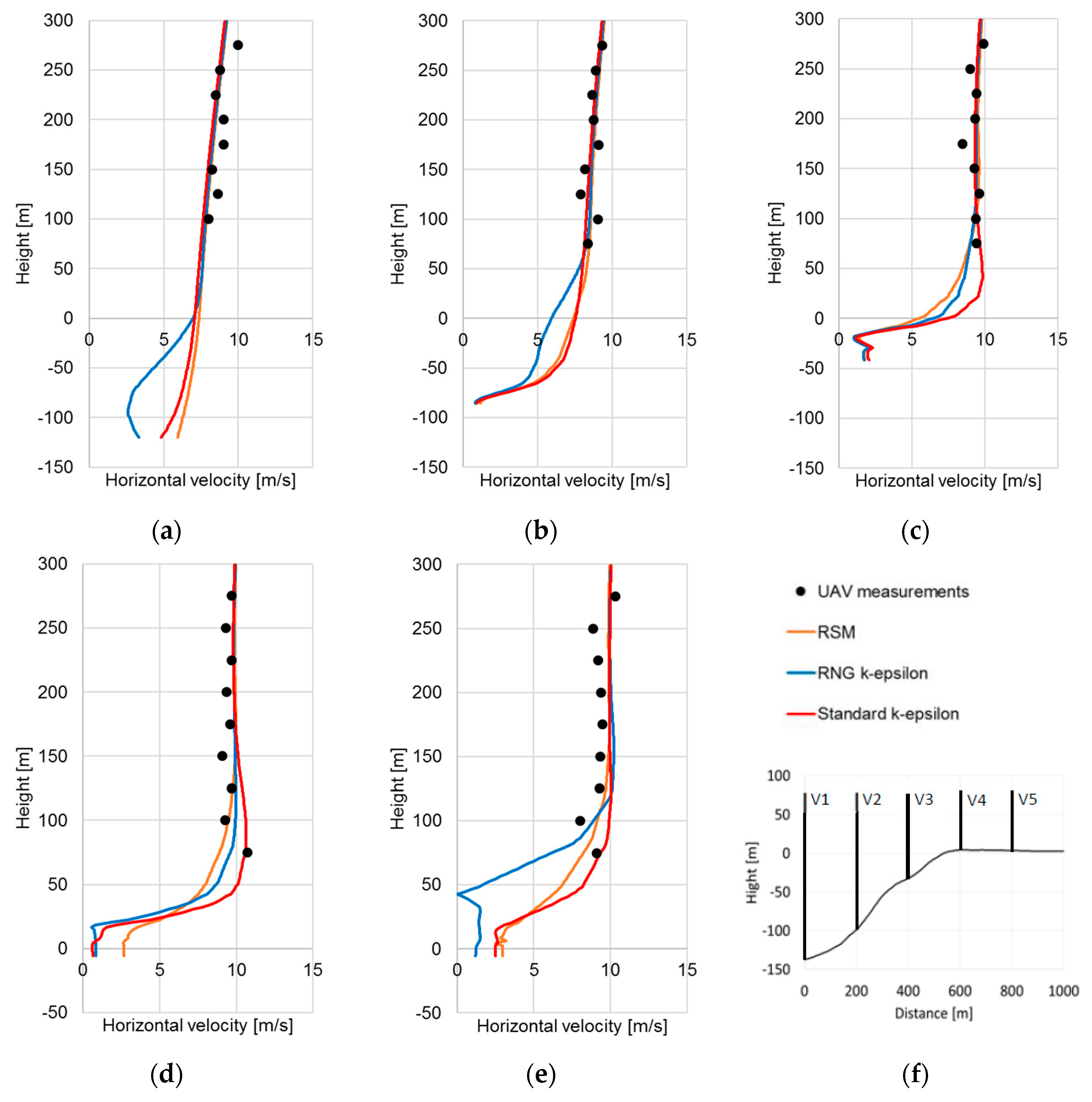
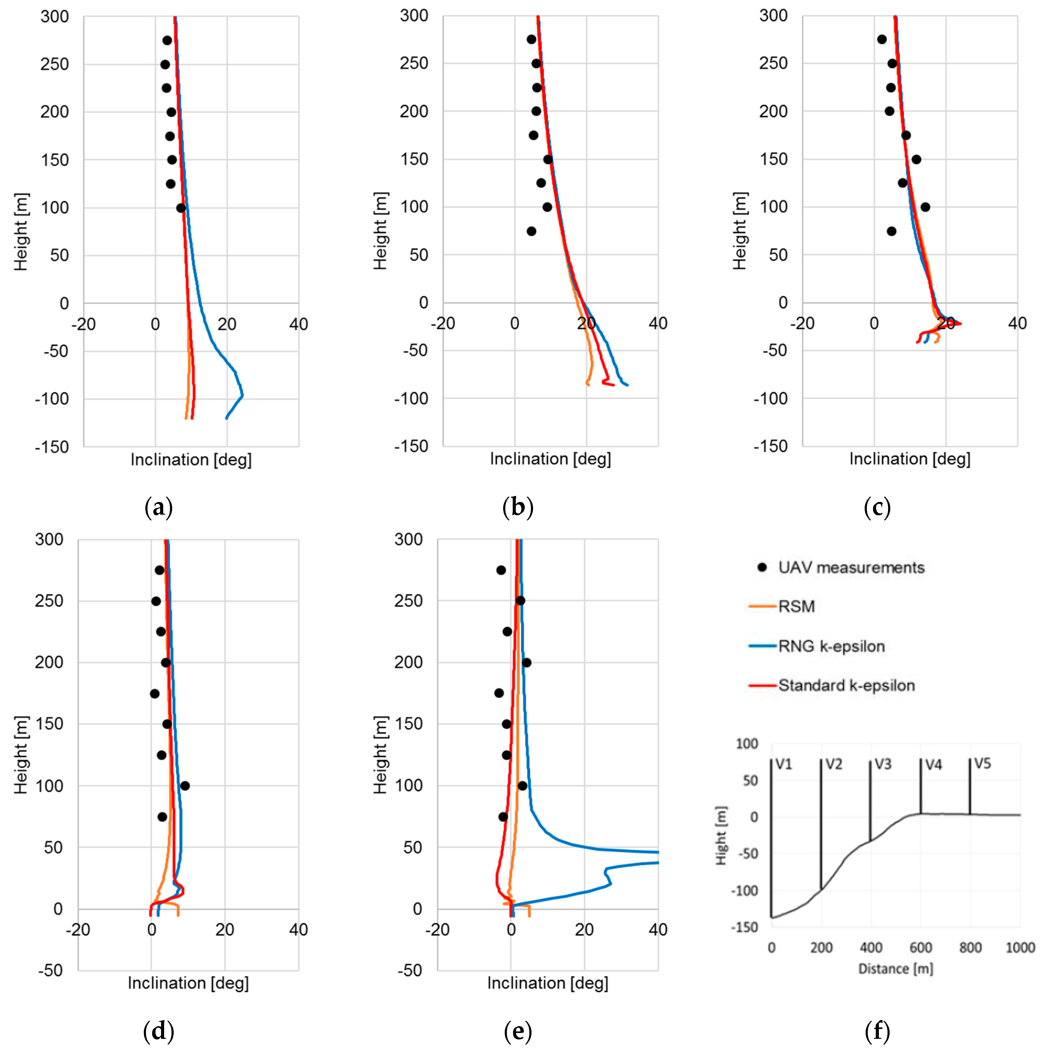
To validate the results quantitatively, the simulations results are also compared with flight data, horizontally averaged at various altitudes. This enables a better understanding of the velocity profiles in the vicinity of the escarpment at the test site. Additionally, the inclination angle of the flow is investigated, providing information about the flow direction in reference to the horizontal plane. Therefore, the results are evaluated along five vertical lines V1–V5, which are arranged perpendicularly along the flight path of the UAV (
Figure 3 and
Figure 10f). As reference, the height at the crest of 660 m a.s.l. is chosen and set to 0 m for the evaluation in
Figure 10 and
Figure 11.
For the RNG k-ε model, the velocities close to the ground are found to be considerably lower along position V1 than for the standard k-ε model and the RSM because the flow separation on the lee side of the hill is predicted larger. This effect still is visible at position V2. In
Figure 10b,c it can be seen that the flow is displaced along the forested escarpment. Therefore, the velocity at the ground is increased, and a strong velocity gradient is developed in the near-wall region. The acceleration is largest for the standard k-ε model. At a distance of 600 m at the crest at position V4, again, the maximum speed is predicted by the standard k-ε model. There, the topography becomes almost flat, which is why the flow tends to separate. The velocity up to a height of 20 m above the ground is already close to zero for the standard k-ε and RNG k-ε models, whereas the flow is still directed more forward for the RSM. This effect is additionally driven because of the forest edge located directly at the crest. Further downstream at position V5, a separation zone with reverse flow is predicted by the RNG k-ε model up to a height of around 45 m. However, this is not the case for the standard k-ε model and the RSM.
From
Figure 10c, the typical velocity distribution within the forest is developed for all turbulence models, as observed in in
Section 3, for the canopy test case of Shaw and Schumann [
14]. Therefore, a local velocity maximum close to the ground and a local minimum at the maximum LAD close to the treetop is observed. This flow distribution disappears for position V4 and position V5 because these positions are located downstream to the forested escarpment.
The simulation results for the horizontal velocities are generally in very good agreement with the measured data. The shape of the profiles and the velocity level can be captured with high accuracy. Unfortunately, there are no measurements available below 75 m above ground from the UAV at present, where the largest differences for the turbulence models are found. However, the interesting heights for the use of wind energy are covered by the UAV measurements. Overall, the most accurate prediction of the velocities is achieved by means of the standard k-ε model and the RSM, resulting in an RMSD value of 0.62 m/s and 0.63 m/s in total for all measuring positions, respectively. However, the agreement for the RNG k-ε model is also on a very good level, giving an RMSD for the horizontal velocity of 0.71 m/s.
Regarding the inclination angle (
Figure 11), the profile along V1 is determined by the wake downstream to the hill in front of the escarpment. The extension of the wake is largest for the RNG k-ε model. Therefore, the flow is directed upwards just upstream to the escarpment in a stronger manner than for the other turbulence models (
Figure 11a). At position V2 depicted in
Figure 11b, the differences when applying different turbulence models can be seen. The flow is displaced in the forested near-wall area, leading to high inclination angles. Again, the inclination becomes largest in the near-wall area for the RNG k-ε model followed by the standard k-ε model and the RSM. The differences diminish at elevations higher than 100 m above ground. For the positions V3 and V4, the differences are quite small for all models and can be observed only in the vicinity of the ground.
At position V5 (
Figure 11e), it is shown that the inclination angle has mostly negative values for the standard k-ε model. Accordingly, the slope of the inclination angle over height is predicted by the RSM, showing slightly higher, positive inclination angles. However, the result for the RNG k-ε model displays high, positive inclination angles in the near-wall area. This difference is due to the reverse flow predicted by the RNG k-ε model at this position.
As for the horizontal velocities, the simulation results and measurements of the inclination angle are in very good agreement. For the standard k-ε model, the smallest RMSD value for the inclination angle is computed (3.12 deg). The RSMDs for the RSM and RNG k-ε model are slightly higher, giving values of 4.51 deg and 4.93 deg, respectively.
5.2.3. Comparison of Simulation Results and Measurements from a Meteorological Wind Mast
Sonic anemometer measurements enable the evaluation of Reynolds stresses by means of high frequency velocity measurements. In the following section, these from measurement devised Reynolds stresses are compared with the Reynolds stresses predicted by the RSM at the position of the meteorological mast. For the comparison, the different time and length scales in the atmospheric flow phenomena are an important issue. Using a single time slice from the weather model COSMO-DE as boundary conditions for the simulations, only turbulence effects of the topography and thermal stratification are captured by the CFD model. The length and time scales of these phenomena are within 1 km and a few minutes, respectively. All other phenomena—for example, convection and diurnal cycle, among others—have much larger time scales (10 min to hours). As long as the difference of these time scales is big, it can be assumed that the quasi stationary time slice approach works relatively well, according to Schlünzen [
38].
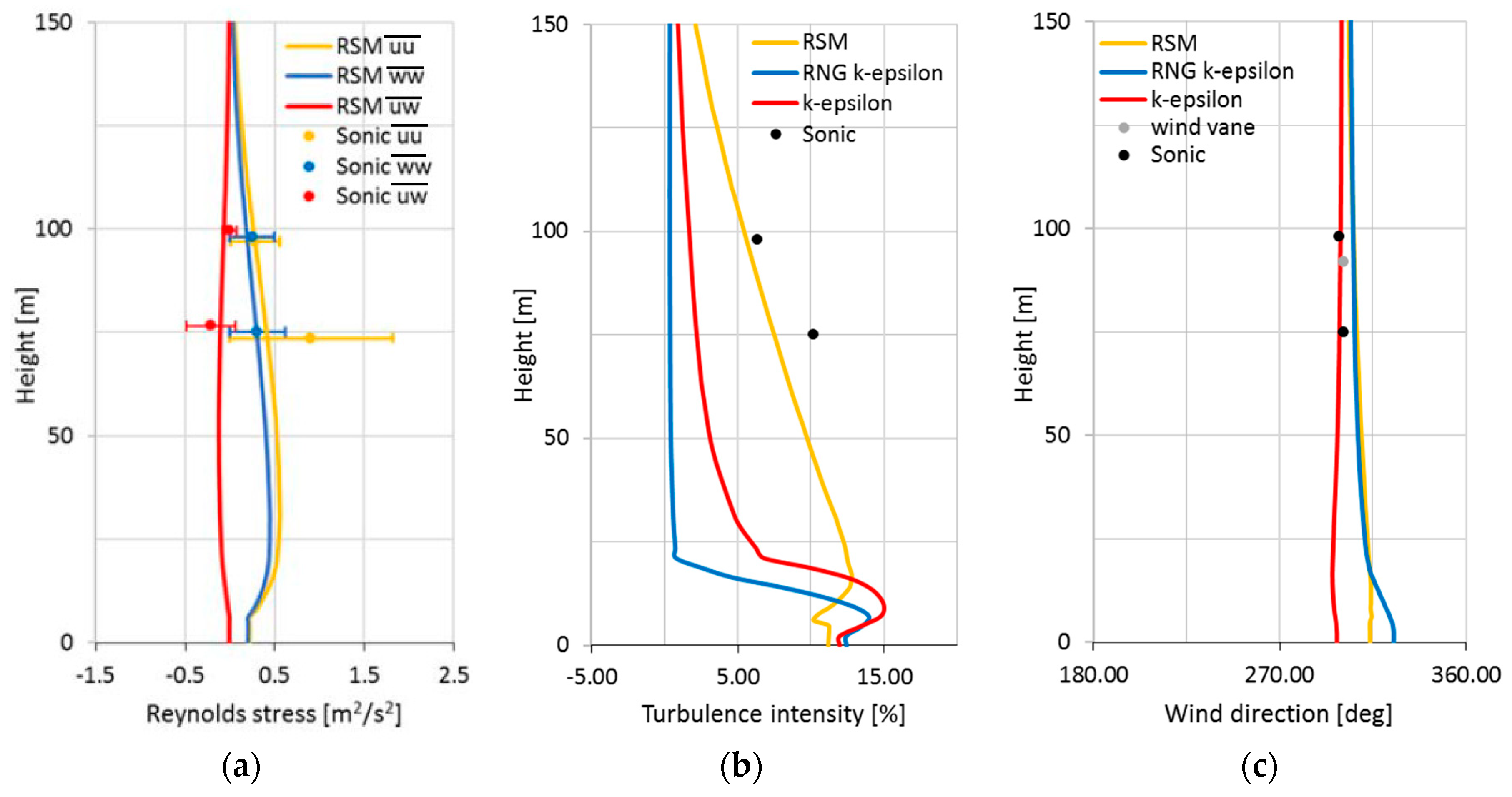
The measurement values are depicted in
Figure 12a–c for the 27 March 2015 at 3:00 p.m., which is the time used for the simulations. As described above, the boundary conditions for the simulations are based on one specific time slice from the COSMO-DE weather model and, therefore, flow phenomena with time scales larger than a few minutes are not captured in the models. To eliminate the phenomena with larger time scales from the measurements, a time averaging of 2 min is applied for the Reynolds stresses, the turbulence intensity, and the wind direction. For the comparison, the co-ordinate system is rotated with the
x-axis pointing in flow direction and the
z-axis perpendicular to the Earth’s surface.
In
Figure 12a, the Reynolds stresses
,
, and
are opposed for the measurements (2 min averages) and simulation results. For all measurements, the mean value and its variance are depicted. The largest deviations occur for the Reynolds stress
at the measurement height of 75 m. Looking at the sonic measurements at the height of 75 m, the variance for the Reynolds stress
accordingly becomes large as well. Despite this, the agreement between simulation results and the sonic anemometer measurements are in good accordance on both measurement levels at constant heights of 75 m and 98 m above ground. Further validation for the Reynolds stresses below 75 m would be desirable. Unfortunately, no measurement data is available at 50 m for this particular date.
The principle Reynolds stresses are used for the computation of the turbulent kinetic energy. From this quantity, the turbulence intensity, which is the measure for the fatigue load of wind energy turbines, is derived for all turbulence models (
Figure 12b). The RNG and standard k-ε models show a higher turbulence intensity close to the ground than the RSM. However, the turbulence intensity decreases rapidly with height. In connection to the measurements, this is a clear indication that the dissipation of turbulence is over-predicted by the two-equation models. Comparing the turbulence intensity, again, a good agreement is found for both measuring levels in the case of using the RSM, showing its potential. However, the turbulence intensity still is under-predicted, especially at the height of 75 m.
In
Figure 12c, the wind direction is depicted for the different turbulence models in combination with the values measured with the sonic at heights of 75 m and 98 m, and a wind vane at a height of 92 m. Only a minor change of the angle over the height between 20 m and 150 m above ground can be observed. This is because of the fact that viscous forces are much bigger in the laminar and Prandtl boundary layers than the Coriolis force. In the immediate vicinity to the ground below 20 m, the results of the RNG and standard k-ε models show a slight increase of the angle. For the RSM and RNG k-ε models, slightly higher values are generally predicted than those for the standard k-ε model. The simulation results are in very good accordance with the measurements for all turbulence models. The standard k-ε model gives the best agreement, whereas the RNG k-ε model and RSM show slightly larger deviations.
6. Conclusions
An formulation of the Navier–Stokes equations based on the Boussinesq approximation was used, considering the stratification of the Earth’s atmosphere and Coriolis force. The Reynolds stress model (RSM) as well as the RNG k-ε and the standard k-ε turbulence models were applied, including additional dissipation and production terms to capture the influence on turbulence in forested areas.
The implementation of the additional capabilities was verified by means of a homogeneous canopy test case. Additionally, the internal canopy time scale was adapted using a coefficient to fit the results of the RSM to the reference solution achieved by LES simulations. A factor of was found to be most appropriate, giving the lowest RMSDs for the normalized horizontal velocity, the normalized turbulent kinetic energy, and the normalized Reynolds stresses with respect to the reference solution. Generally, a very good agreement for all turbulence models was achieved regarding the predicting of the wind velocity. Differences in the turbulent kinetic energy are more apparent, and show that the best agreement occurs when the RSM is used. Most striking is that the maximum of the turbulent kinetic energy just above tree top is well in accordance with the reference solution for the RSM, whereas for the RNG k-ε model and standard k-ε models, the turbulent kinetic energy is over-predicted.
In a second step, the wind flow for the WindForS wind energy test site with partly forested complex terrain in Stötten near Geislingen an der Steige, southern Germany, was simulated, with the goal of model validation for this specific location. In particular, data from the 27 March 2015 at 3:00 p.m. were selected, linked to the most frequently occurring north–west wind and dry, near-neutral conditions. The orography and flora were described using digital height and digital landscape models. For the computations, boundary conditions were derived from the COSMO-DE weather model. The simulation results were compared with measurements from an unmanned aerial vehicle (UAV) and from a meteorological mast using sonic anemometer.
Generally, for the RSM, the RNG k-ε model, and the standard k-ε model, a very good agreement was achieved for predicting horizontal wind velocities and inclination angles in comparison to the UAV measurements. The very good agreement was confirmed by the RMSDs for the horizontal velocities of 0.71 m/s, 0.63 m/s, and 0.62 m/s along vertical measurement locations, respectively. The smallest RMSD value of 3.12 deg was computed using the standard k-ε model. The RSMDs for the RSM and RNG k-ε model are slightly higher, giving values of 4.51 deg and 4.93 deg, respectively.
Sonic anemometer measurements were used to validate the turbulent quantities. It was shown that only the RSM managed to predict the turbulence intensity with high accuracy. Using the RNG k-ε and standard k-ε models, the turbulence intensity prediction was far too low. It was found that the turbulent kinetic energy downwind of obstacles like hills or the escarpment dissipates much faster for the RNG k-ε and standard k-ε models than for the RSM connected to an under-prediction of the turbulence intensity. Furthermore, it was confirmed by the RSM model that turbulence becomes anisotropic in the complex terrain, mainly driven by the orography. For these reasons, the RSM is the best choice for RANS models to predict fatigue load on wind turbines in complex terrain.
It was shown that by means of one-way coupling of the CFD code with the weather model COSMO-DE from German Meteorological Service, appropriate boundary conditions for the simulations can be initialized, enabling the prediction of the inhomogeneous flow situation with high velocity gradients along and perpendicular to the main flow direction in complex terrain with high accuracy. For this reason, different nested domains with increasing spatial resolutions were devised to capture influences on the flow in the far field of the test site in an appropriate manner.
For the model validation, a homogeneous forest canopy was assumed. The LAD was used according to Shaw and Schumann [
14] in combination with a mean forest height. However, the canopy morphology may also have an impact on the wind flow [
39]. Unfortunately, as often this data is not available for the WindForS test site at present and, therefore, this aspect could be part of future investigations. Because this validation took place under thermally near-neutral conditions and only uses a short period of data, it is essential to investigate the accuracy of the model chain under thermally stable or unstable conditions, as this can impact the generation and dissipation of turbulence in the atmosphere both locally and further afield. Finally, transient effects due to diurnal changes in the atmosphere have to be studied. Therefore, further UAV measurements at lower heights above the Earth’s surface are planned within the BMWi-funded project WINSENT, further validating the simulation code for the prediction of wind flow at the WindForS test site and in complex terrain in general. Additionally, Lidar measurements as well as 3D-ultrasonic and cup anemometer measurements from four meteorological masts are going to be provided. This will enable further, more detailed investigations of the wind flow, and particularly the turbulence, especially in the Prandtl layer of the atmosphere. However, for the understanding of the main flow phenomena and the characterization of the test site for the use of wind energy, the approaches investigated so far are already valuable tools, which are going to be operationally utilized for the planning of the following measuring campaigns and the layout and construction of the wind test site.


