LES and Wind Tunnel Test of Flow around Two Tall Buildings in Staggered Arrangement


1
Department of Civil Engineering, The University of Hong Kong, Pokfulam Road, Hong Kong, China
2
Department of Civil and Environmental Engineering, The Hong Kong University of Science and Technology, Clear Water Bay, Hong Kong, China
*
Author to whom correspondence should be addressed.
Computation 2018, 6(2), 28; https://doi.org/10.3390/computation6020028
Submission received: 30 January 2018
/
Revised: 19 March 2018
/
Accepted: 20 March 2018
/
Published: 23 March 2018
(This article belongs to the Special Issue Computational Methods in Wind Engineering)
Abstract
:Wind flow structures and their consequent wind loads on two high-rise buildings in staggered arrangement are investigated by Large Eddy Simulation (LES). Synchronized pressure and flow field measurements by particle image velocimetry (PIV) are conducted in a boundary layer wind tunnel to validate the numerical simulations. The instantaneous and time-averaged flow fields are analyzed and discussed in detail. The coherent flow structures in the building gap are clearly observed and the upstream building wake is found to oscillate sideways and meander down to the downstream building in a coherent manner. The disruptive effect on the downstream building wake induced by the upstream building is also observed. Furthermore, the connection between the upstream building wake and the wind loads on the downstream building is explored by the simultaneous data of wind pressures and wind flow fields.
1. Introduction
Interference effect has been found to cause significant modifications to wind loading of a building being surrounded by neighboring buildings. Interference effects on wind forces have been thoroughly studied by wind tunnel experiments [1,2,3,4,5]. In the last few years, local wind pressure modifications have also attracted some attention due to the importance in cladding design [6,7,8]. Through numerous previous studies, large amounts of useful data have been obtained to enrich the database of interference effect and some empirical formulas have been proposed to estimate interference effects on local and overall wind loads for certain building geometries and arrangements.
Many parameters can modify wind loads induced by interference from surrounding buildings, such as geometry and arrangement of buildings, terrain type and turbulence intensity of approaching flow. Possible combinations of these parameters are extremely large and, thus, are impossible to be covered exhaustively. Therefore, a more physically-based approach, such as investigating the underlying mechanisms of interference effect, would be worth adopting to solve the problem.
Some efforts have been made to understand various interference mechanisms. Bailey and Kwok [1] measured the velocity spectrum in the wake of a tall building model with and without an identical upstream building in tandem arrangement and found that the periodic vortex shedding was obvious for the isolated building but totally disappeared for the building with an upstream building. They concluded that the upstream building had a disruptive effect on the vortex shedding of the downstream building. Under this situation, the across-wind fluctuating energy on the downstream building mainly came from the approaching flow. This finding was confirmed by flow visualization experiments conducted by Taniike [9] which also found that fluctuating drag on a downstream building increased as the size of the upstream building increased because the larger building width increases the scale of the shed vortices. Sakamoto and Haniu [10] observed the reattachment of shear layer of an upstream building onto the side surface of the downstream building in several different staggered arrangements by smoke visualization technique. Gowda and Sitheeq [11] visualized the flow pattern between two tandem twin buildings and found that the downstream building experienced three stages, namely, submergence in the shear layers, being attacked by the shear layer directly on the windward surface and insusceptibility to the interference, as the spacing between two buildings changed from small to large values. Hui et al. [12] observed the flow pattern between two rectangular-section high-rise buildings and found that peak pressure on the downstream building were usually caused by the shear layer from the upstream building. Findings in many of the above-described studies are made from flow visualizations in which wind flow pattern between two tall buildings and its possible connection with resulted wind load were qualitatively observed and analyzed. However, the exact interference mechanisms between two high-rise buildings remain unclear. More detailed investigation of the wind flow field around buildings and its relationship with the wind forces may provide more understandings of the interference mechanism.
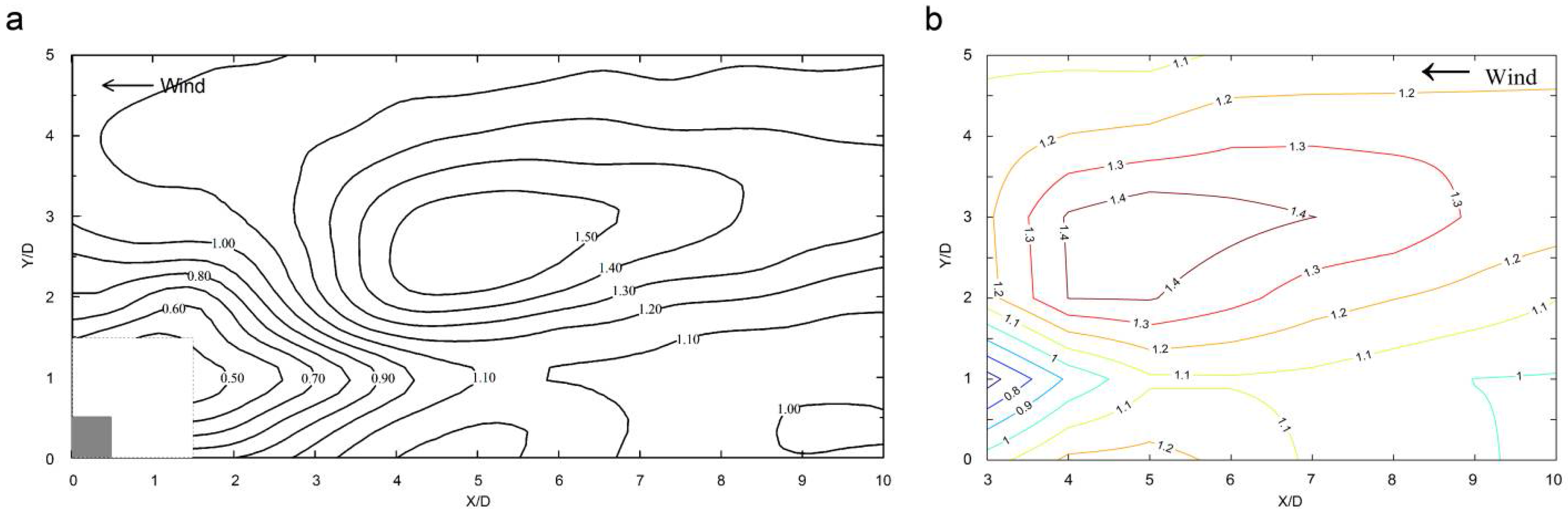
With the development of computers, since the 1990s, researchers began to employ Large Eddy Simulation (LES) to study the highly time-dependent wind flow and wind loads of building structures. Various benchmark study of LES on buildings has been carried out to validate numerical results with wind tunnel experiments [13,14,15] with satisfactory agreement. However, in a real urban environment, tall buildings are usually built in proximity rather than being alone. For such complex situations, there has not been a systematic study validating the accuracy of LES. When two tall buildings are closely built, the strongest interference on across-wind force on the downstream building is reported to occur when the streamwise distance of two buildings is 5D and the transverse distance is 2.5D, where D is the width of the building [16]. Figure 1 reproduces the results of [16] on the contour map of interference factors (IF) of Root-Mean-Square (RMS) across-wind force on the downstream building with the upstream building at various relative locations (X, Y). The IF is defined as the ratio between the RMS across-wind force on the building under interference and the same force on the building in the isolated single building situation. Very similar contours of IF have also been measured by the present authors in the wind tunnel [17], and the results are reproduced in Figure 1. The wind flow behavior and excitation mechanism for the largely magnified RMS across-wind force have not been studied in detail. This is partly due to the difficulties in obtaining simultaneous data on the fluctuating wind pressures on the buildings and turbulent wind fields past the building. While the present authors have attempted to use advanced measurement techniques to investigate the problem in the wind tunnel [17], unsteady CFD computation with LES is a promising tool to explore the flow-structure interaction. The present study chooses the critical arrangement of peak across-wind interference between of the two buildings in staggered arrangement for LES prediction to investigate the flow structures around two tall buildings and the excitation mechanism of building interference.
In this study, firstly, the LES method was applied to study the dynamic wind flow field around two staggered tall buildings in the critical arrangement for across-wind interference (X/D = 5, Y/D = 2.5). Then, the flow field around two staggered tall buildings is measured by time-resolved particle image velocimetry (TR-PIV) with synchronized pressure measurement on the downstream building. The flow characteristics between the simulated results from the LES method and those obtained from the wind tunnel test were compared to validate the simulated numerical results. Finally, the flow structures around the two buildings are further investigated aiming to bring about a better understanding of the interference effect.
2. Simulation on Shear Stress/Friction Velocity on Roofs
2.1. Governing Equations
The numerical simulations in the present study were performed using commercial CFD software Ansys Fluent [18]. In the LES turbulence model, large-scale eddies are explicitly resolved by solving the filtered Navier–Stokes equations whereas only small eddies are modelled. The governing equations of LES are obtained by filtering the time-dependent Navier–Stokes equations as follows:
where and are the filtered mean velocity and the filtered pressure respectively, and are the air density and the dynamic viscosity, respectively, and is the subgrid-scale stress which is modeled as follows:
where is the subgrid-scale turbulent viscosity, and is the rate-of-strain tensor for the resolved scale.
The Smagorinsky-Lilly model [19] is used for the subgrid-scale turbulent viscosity, where the eddy viscosity is modeled as follows:
where is the mixing length for subgrid-scales, is the von Karman constant, is the distance to the closest wall and V is the volume of a computational cell. The dynamic version of the Smagorinsky model [20] was employed in the present study, and Cs is computed at each time step with a test-filter and clipped to the range of 0 to 0.23 to avoid numerical instabilities. This imposed maximum value of 0.23 for Cs follows the default value in Ansys Fluent and is found to be appropriate for flow around an isolated bluff body [21].
2.2. Computational Domain and Boundary Conditions
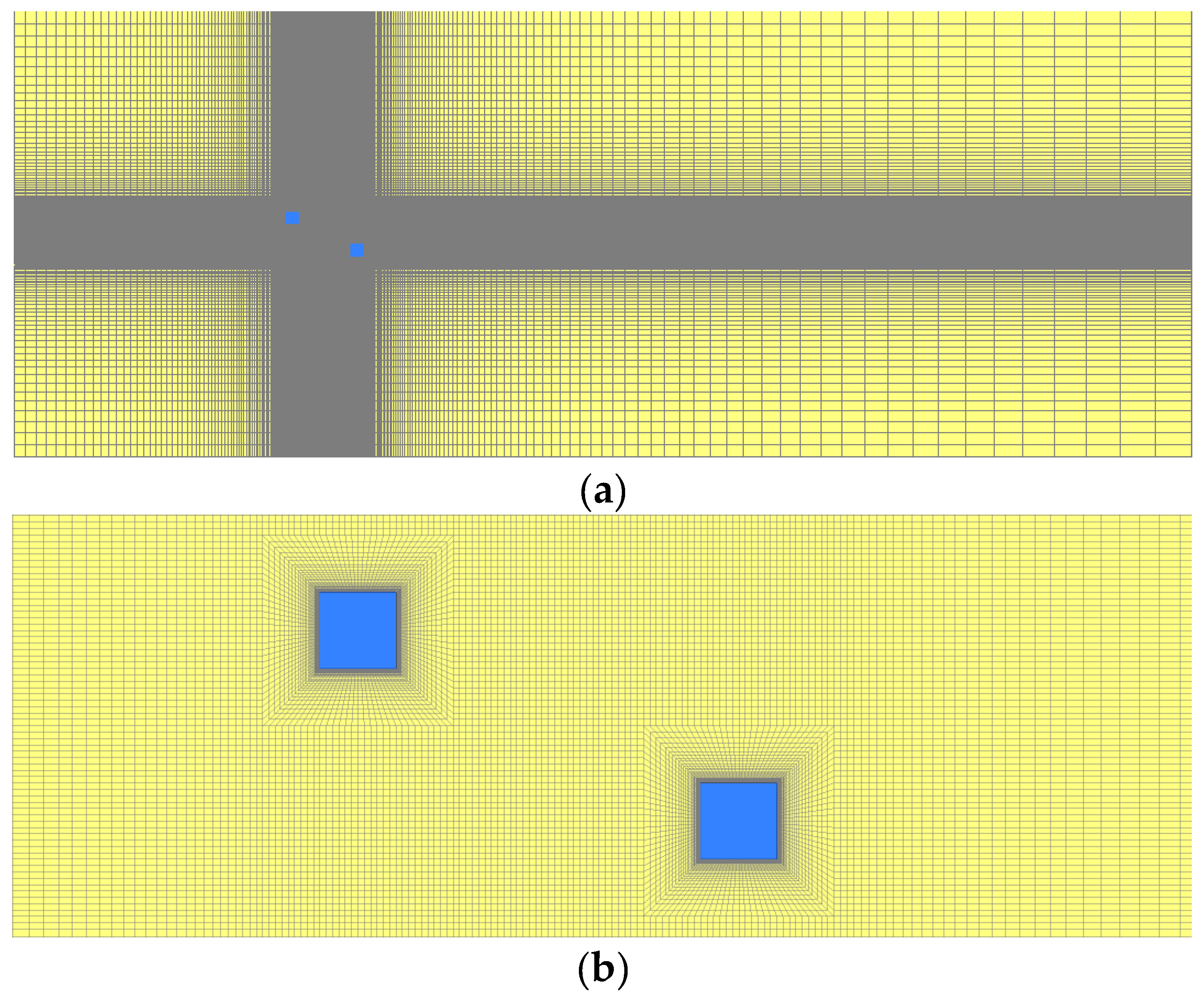
The numerical simulations were conducted on two identical tall building models to compare the simulated wind flow around two tall buildings with that obtained from the wind tunnel experiment, which will be described in later sections. Both building models had a square-plan form of breadth D = 30 mm. The height-to-breadth ratio was H/D = 6. At the target geometric scale 1:1000, the models represented full-scale buildings of height 180 m and width 30 m. Figure 2 shows the computational domain and the study model. The length, breadth and depth of the computational domain were 16.7H, 34.5D and 3H, respectively, which follow the recommendation by Franke [22] and COST [23]. The distance between the windward face of the upstream building and the inlet was 5H. The outlet boundary was 10H away from the leeward face of the downstream building to allow flow re-development behind the wake region. This computational domain was discretized into 4.8 × 10⁶ hexahedral meshes, which is refined near the target building and ground surface. The height of the first layer of cells around the building models was small enough (y+ < 1) to solve the viscous sublayer. Stretching ratios between neighboring cells were kept below 1.3 in accordance with the best practice guidelines [23,24].
A time-dependent velocity profile was imposed at the inlet boundary targeting at that obtained from the wind tunnel test. The inflow turbulence was generated by FLUENT inherent vortex method and the kinetic energy of turbulence and the dissipation rate at the inlet section were calculated by
where u(z) is time-averaged wind velocity at height z; k(z) is turbulent kinetic energy; (z) is dissipation rate; Cμ is a model constant of 0.09. The amount of vorticity was set to 50.
Symmetric boundary conditions were imposed at the sides and the top boundary of the domain, thereby implying zero normal velocity and zero gradients of all variables at the boundaries. Zero static pressure was imposed at the outlet of the domain. The building and ground surfaces were defined as non-slip wall boundary condition.
All the discretized equations were solved in a segregated manner with the pressure implicit with splitting of operators (PISO) algorithm. A second-order accurate bounded central-differencing scheme was used to discretize the convection term in the filtered momentum equation. Second order discretization schemes were adopted for time and spatial discretization. The simulation was initialized with the solution of a preceding RANS (Reynolds-averaged Navier–Stokes) simulation which allows fast convergence of computation. After an initialization period Tinit = 3.0 s, the statistics were sampled for 20 s, corresponding to 38.7 flow-through times (Tft = Lx/UH, where Lx is the length of the computational domain), which are longer than the sampling duration suggested by Gousseau [21] who found that 21.8 flow-through times are sufficiently long to achieve statistical convergence.
3. Description of Wind Tunnel Test
The simulated wind flow field by LES is validated by comparison between the wind tunnel experiments that were carried out in the boundary layer wind tunnel in the Department of Civil Engineering at the University of Hong Kong. The working section of the tunnel was 3.0 m wide, 1.8 m tall and 12 m long. Wind tunnel tests were carried out under simulated wind flow of the open land terrain, where the mean wind profile followed the power law with a power exponent of 0.11 [25]. The mean wind speed and turbulence intensity at the height of the building model during the test were UH = 5.8 m/s and 0.089, respectively. The measured mean wind velocity and the turbulence intensity profiles in the wind tunnel test and the simulated profiles in the numerical simulation are presented in Figure 3. The longitudinal integral scale of turbulence was about 0.39 m at the roof height in the wind tunnel. This corresponds to a full-scale integral scale of 390 m at 180 m height.
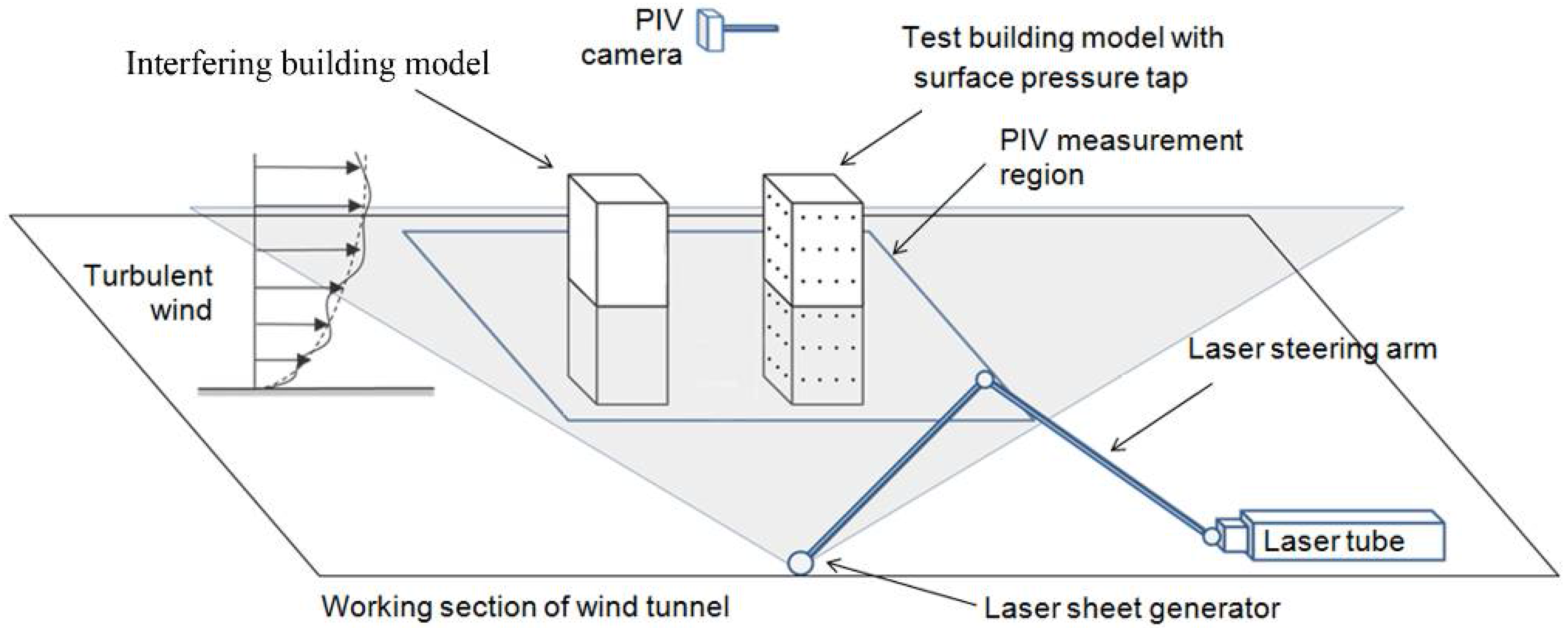
A total of 120 pressure taps, 20 on each of its six layers (Level 1 to 6 from the roof to the bottom), were installed on the walls of the test building as shown in Figure 4. A time-resolved PIV system measured the instantaneous velocity fields on a horizontal plane through the two buildings. The measurement plane was illuminated by a thin laser sheet generated from the laser beam of a double-cavity Q-switched Nd:YAG laser (Nano 50–100, Litron). The laser sheet generator and the laser steering arm were placed inside the working section of the wind tunnel and downstream of the building model. A 1:1 mixture of DEHS liquid and sunflower seed oil was used to produce seeding particles using a high-volume liquid seeding generator (10F03, Dantec Dynamics). The particles had diameters at about 2 to 5 μm and could satisfactorily scattered the laser light in the air flow when viewed as a small region of interest. Flow images were captured with a high-speed CMOS camera (SpeedSense, Dantec Dynamics). The camera had a high sensitivity for the weak scattered light signals in air flow with resolution at 1920 × 1200 pixels. The camera framing speed was set at 100 double-image/s to capture a time sequence of particle images of 1825-image length. A time interval 0.12 ms was used between the double laser pulses to fix the initial and final positions of seeding particles in the double image. The PIV analysis software was based on the adaptive PIV algorithm [26,27]. In the final iteration, PIV vectors were obtained on interrogation areas of size 16 × 16 pixels. The number of velocity vectors were 120 × 75 and the physical resolution of each vector was about 3.2 × 3.2 mm2. With this configuration, the measurement uncertainty of individual velocity vector was estimated at about ±0.02UH [28,29].
To synchronize the pressure measurement and flow field acquisition by PIV, pressure measurement was triggered by the framing signals of the PIV camera. This synchronization ensured that the pressure scanning was made at the same instants when the PIV camera captured the double-images of the flow and that both sampling was made at 100 Hz. Figure 5 shows the PIV set-up in the wind tunnel.
4. Result Analysis and Discussion
4.1. Time-Averaged Wind Flow Characteristics
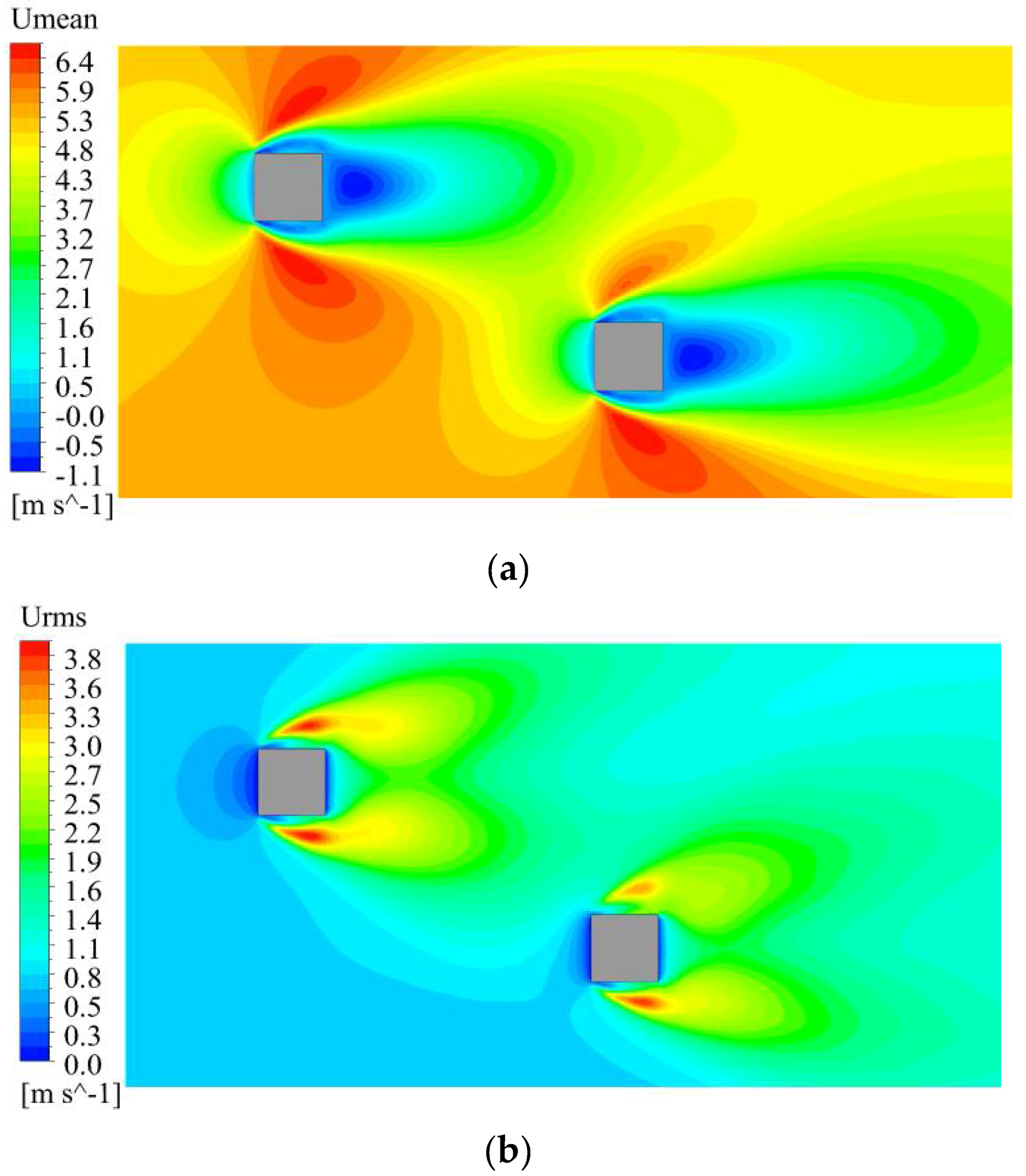
Time-averaged mean and RMS horizontal flow fields at half building height by LES are shown in Figure 6. Two antisymmetric building wakes are observed behind the two buildings. The upstream building wake slightly swings upward due to the presence of the downstream building. In addition, the upper separating shear layer of the downstream building is found to be weaker than its counterpart in both mean and fluctuating contours.
Figure 7 presents time-averaged streamlines by LES and wind tunnel test. The LES flow pattern agrees well with that obtained from wind tunnel test. A distinctively different wake pattern is observed on the downstream building. The mean flow approaching the building is shifted in a slightly sideway direction (or downward direction in the figure). As a result, the clockwise vortex at the upper side wall is suppressed largely by the downwards-shifted shear layer, while, the anti-clockwise vortex, which is supposed to appear near the lower side, is impaired dramatically in the time averaged sense. The recirculating region of the wake now occupies a smaller space up to a length of 1.7D from the center of the building, comparing with an isolated building wake of which the recirculation area is supposed to be extended to 2.2D [29]. As for the upstream building, the building wake pattern remains largely unchanged except for the slight upward bifurcation line.
4.2. LES Validation by Wind Tunnel Result
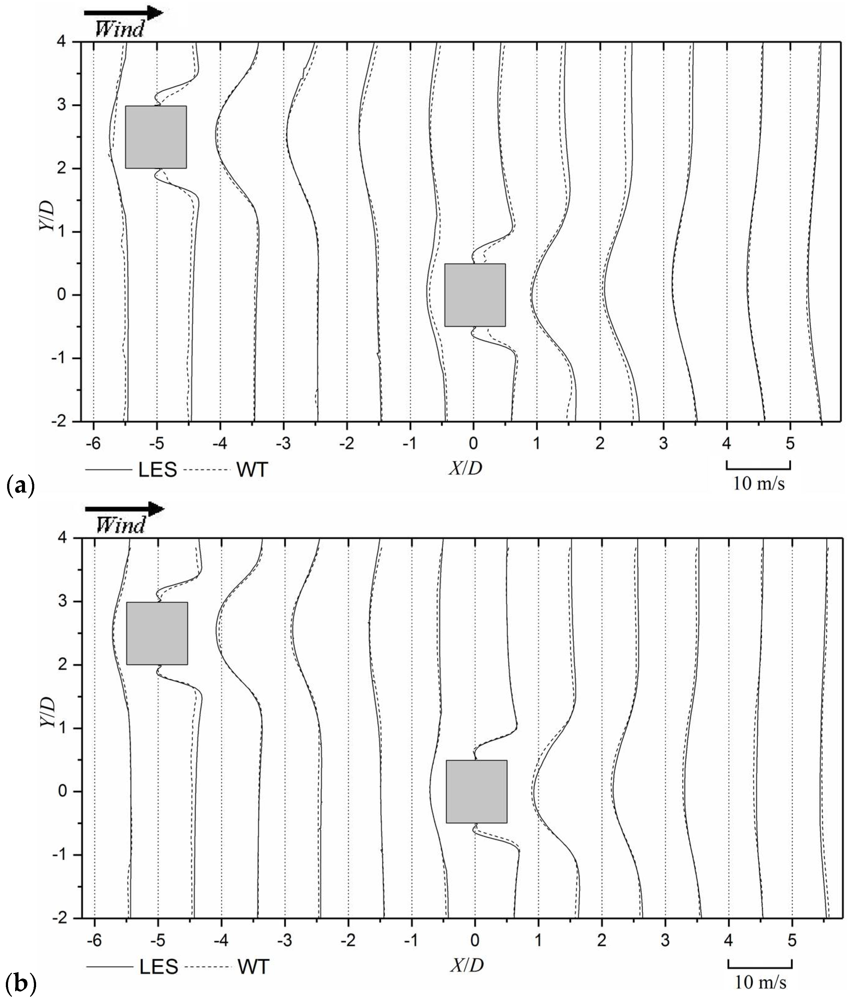
To validate the results of LES, the simulated values of the wind velocity around two building models are compared with those measured in the wind tunnel test by PIV. Figure 8 presents the profiles of the mean along-wind wind velocity at the planes of half building height and near the building roof (h/H = 0.82). In this and the following figures, measurements of wind velocity in the wind tunnel by PIV at X/D = −6, −5, −4, −3, −2, −1, 0, 1, 2, 3, 4, and 5 are selected to validate the LES results. For each location, the axis is denoted by a longitudinal dotted axis, which is also acting as the origin for wind velocity plotted transversely with positive values on the right side of the axis and negative on the left. Generally, a good agreement is found between the LES and the wind tunnel test.
The time-averaged mean transverse velocity in building wakes is plotted in Figure 9. A relatively larger difference between the numerical and the experiment results is observed for the transverse velocity than that of the streamwise velocity. The transverse component of the flow approaching the downstream building is mainly negative, indicating a downward sideway direction, which coincides well with the time-averaged streamlines in Figure 7. Because of the flow separation, the vertical component of wind velocity is positive near the upper side walls of the two buildings and negative near the opposite sides. It can be observed that the transverse velocity of the upper separating shear layer of the downstream building is larger than that of the upstream building, which means the flow separation from the side wall close to the upstream building is enhanced by the upstream building.
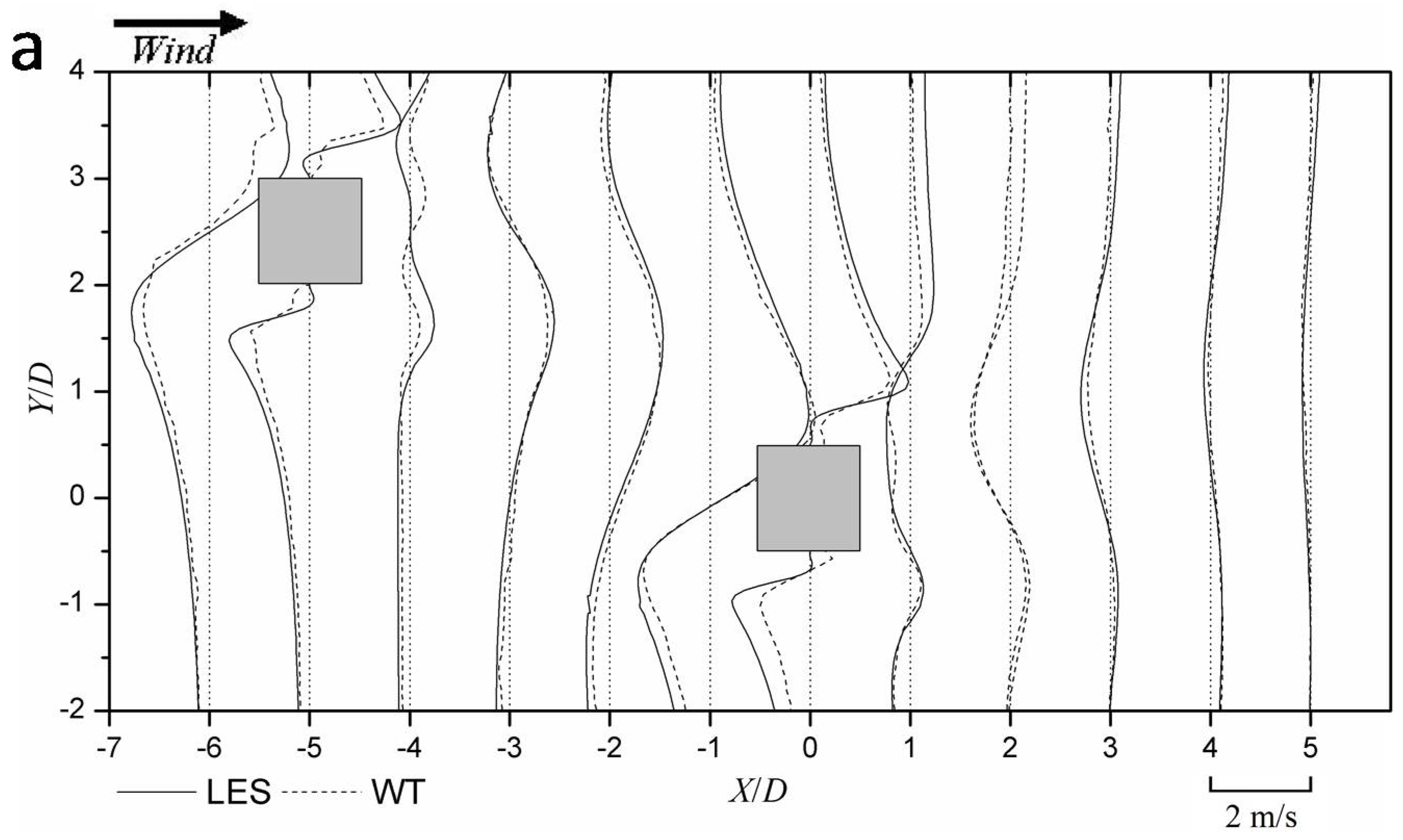
The distributions of RMS wind velocity components u’ are presented in Figure 10. The distributions of u’ at two horizontal planes are quite similar. The strong fluctuations of separating shear layers result in large RMS values around both sides of the buildings. The main discrepancy between the numerical and experiment approaches lies in the prediction of the near wakes. LES tends to overestimate the streamwise fluctuating velocity in both building wakes.
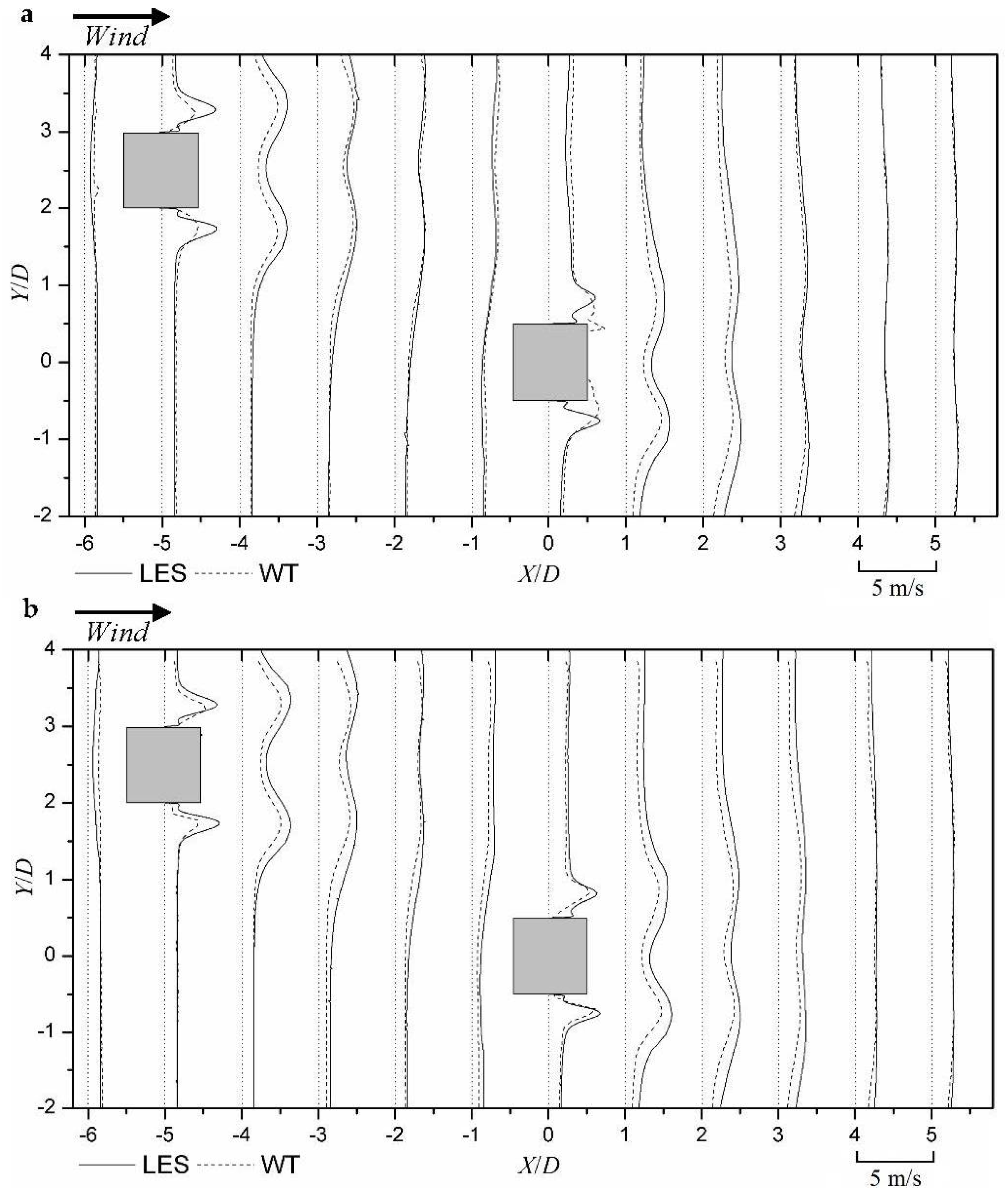
Figure 11 shows results of fluctuating transverse velocity v’ by two methods. Similar with streamwise component u’, the LES results are slightly larger than the wind tunnel results in the near wakes of the two buildings. In these near wake regions, peak values of component v’ are achieved due to the strong direction shift induced by the building wake oscillation.
Generally, there is a very good agreement between the LES predictions and the wind tunnel measurements, especially for the time-averaged mean velocities. Wind velocity distributions at different heights are observed to be quite similar. In addition, the differences between two methods are similar at different heights.
4.3. Vortex Structures of Tall Buildings under Interference
It is known that, for an isolated square cylinder, spanwise vortices shed alternatively from both sides of the cylinder and dominates the near wake region [30]. Although the wind loads on buildings in group are thoroughly investigated, the vortex structures of buildings under interference are still unclear. This section intends to investigate flow structures of two tall buildings in proximity.
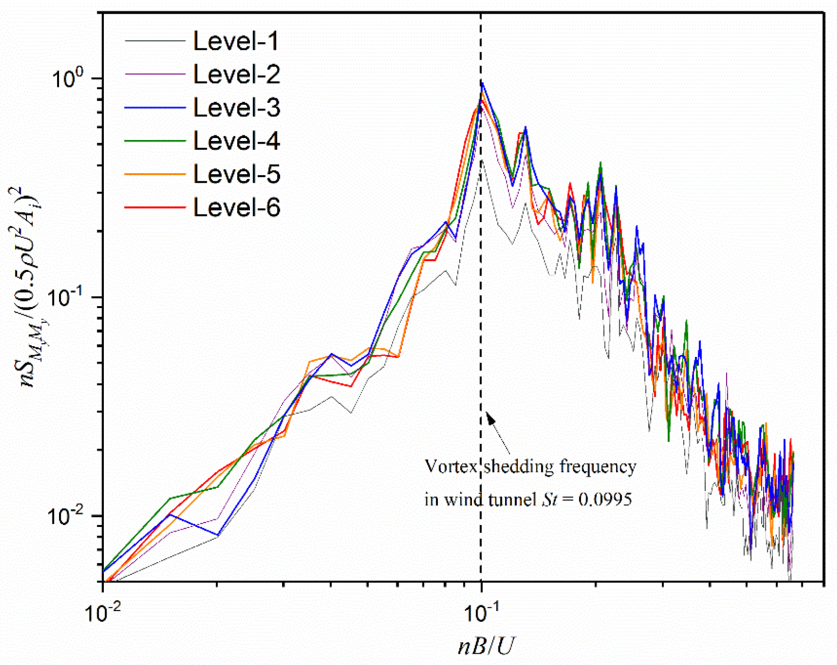
The normalized spectra of across-wind force acting on different heights along the building by LES are presented in Figure 12. Generally, these force spectra of each elevation have quite similar shapes. An obvious peak can be observed for the across-wind forces for all heights around the St = 0.105. This observation is same as wind tunnel results of which the local Strouhal number is 0.0995. Similar values of Strouhal number are found for the across-wind excitation on an isolated building [4,31]. The presence of the upstream building does not change the vortex shedding frequency of the downstream building. The local Strouhal numbers at different heights are approximately the same, and thus the vortices formed from the two sides of the building are shed periodically at a single frequency along the building height.
An attempt to reveal the dominant large-scale coherent characteristics of the LES flow field during the occurrence of peak across-wind forces on the downstream building is made using the conditional sampling method [32]. A peak across-wind force event on level i was determined by a peak in the force time history with magnitude above a trigger level. The trigger level was set using a “peak factor” g and the root-mean-square value of across-wind force coefficient :
with zero mean across-wind forces and by using g > 0 or g < 0, both the peak across-wind force events in either of the two sideway directions could be identified and used as triggers for the conditional sampling. The value of g affects the stringency of peak event selection. For a signal with a Gaussian distribution, a peak factor of magnitude between 2 and 3 has been shown to be appropriate [32]. In this study, a less stringent value of g > 2 or g < −2 was chosen to increase the ensemble size of peak load events.
Figure 13 shows the conditionally sampled wind velocity fields and wind pressures on the horizontal plane at mid-height (h/H = 0.5) corresponding to the instants of peak maximum and minimum across-wind forces. An interesting in-phase synchronization phenomenon is observed for two building wakes. At peak maximum event, a clockwise rotating vortex is about to be shed from the upper side of the downstream building. At the same time, a similar large vortex is observed at the rear side of the upstream building at almost the same phase of shedding.
In Figure 13b, two counter-clockwise vortices dominate the near wake regions. The two in-phase vortices at peak minimum event together with those at maximum event recommend a highly synchronized relation between vortex shedding processes of the two buildings. It is worth noting that the developed vortex on the upper side of the downstream building is farther from the building as compared with the alternating vortex developed from the upper side (Figure 13a). This may contribute to the asymmetric mean flow pattern of the downstream building as observed in Figure 7.
Figure 14 presents the instantaneous three-dimensional flow fields at two typical events corresponding to positive across-wind forces on the downstream building (Figure 14a–c), which is upward in Figure 14c and negative across-wind forces on the downstream building (Figure 14d–f), which is downward in Figure 14f.
For the positive force event, the flow pattern in Figure 14a is similar with that of the peak maximum event (Figure 13a), where two clock-wise vortices are observed to start to shed from the upper side walls of the both buildings. It can be seen that, although the buildings are wholly immersed in the boundary layer where streamwise velocity varies with height, for the both buildings the vortices at different heights develop and shed as a whole. Similar situations are also observed for the negative force event, where counter-clockwise vortices from the both buildings occupy the near-wake regions. For both events, in-phase synchronization phenomenon is also observed, resembling the conditional sampling results (Figure 13).
4.4. Excitation of Across-Wind Forces on Buildings
Vortex excitation described in the preceding section causes fluctuating across-wind forces on the tall buildings. Figure 15 shows the local RMS across-wind force coefficients at each level of the buildings which is integrated from the wind pressures on the corresponding level. Data are shown for the LES computations and wind tunnel tests. The simulated across-wind forces on the upstream and downstream buildings are denoted as “LES-upstream building” and “LES-downstream building”, respectively. The across-wind forces measured on the downstream building in the wind tunnel are marked “WT-downstream building”. For the reference case of the tall building without any surrounding buildings, the local across-wind forces are shown as “WT-isolated building”.
For the upstream building, the across-wind forces from LES are close to those measured on an isolated building in the wind tunnel. The local wind forces have the largest value at about mid-height of the building and decrease gradually towards both the roof and the bottom of the building. As for the downstream building, the smallest local across-wind force also occurs near the roof and then increases gradually with decreased height. This trend is also observed in the wind tunnel results. Both the LES and wind tunnel results show that the across-wind forces on the downstream building are largely magnified due to interference. The across-wind forces from LES, however, are obviously smaller than those from the experiment, especially for the lower half part of the building under interference. The reason for this disagreement is not known and needs future investigation.
Figure 16 shows some instantaneous across-wind forces on the two buildings from the LES results. It is evident that both force signals are characterized by obvious quasi-periodic fluctuations. This feature is also observed on the force signals obtained from the wind tunnel tests, but the data are not shown for brevity. For the across-wind force signal on the downstream building, the positive peaks have evidently larger magnitudes than the negative peaks, while the across-wind force signal on the upstream building fluctuates very symmetrically around the zero value. This indicates that the suction pressures acting on the upper side face of the downstream building (on the side facing the upstream building) are stronger than those acting on the lower side face. Moreover, the across-wind forces on the both buildings are found to fluctuate together in a largely synchronized manner over most periods, although small phase shifts in the in-phase relationship occur occasionally.
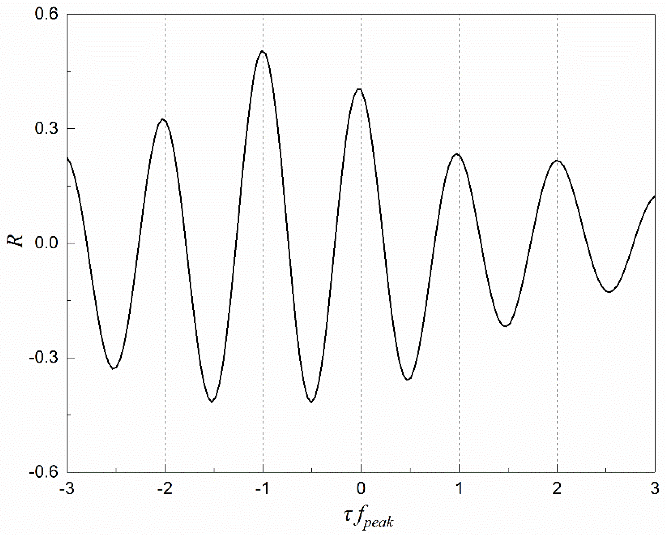
This near in-phase synchronization of the across-wind forces on the two buildings is further confirmed by correlation analysis. Figure 17 shows the time-lagged cross correlation curve R(τ) between the across-wind forces on the upstream and downstream buildings. One peak in the correlation coefficient curve occurs at time lag near τ = 0 with R = 0.40. This indicates that the across-wind forces on the two buildings are positive correlated in time, which agrees well with the flow field results in Figure 13 and Figure 14. The largest peak correlation is found to occur at τ = −1/fpeak, where fpeak is the averaged dominant frequency of the quasi-periodic components in the across-wind force signal (Figure 16). This means that a quasi-cycle of the across-wind force on the downstream building has the strongest correlation with that on the upstream building happened one period earlier. The reason for this becomes evident from the flow excitation mechanism revealed in Figure 13. When a vortex is shed from the upstream building and subsequently convects downstream, the vortex dynamics causes flow oscillations in the building wake. When these oscillations reach the downstream building, they act to enhance flow separations on the building which is then responsible for the magnification of the across-wind force on it. As a result, the across-wind force signal on the downstream building relates to vortex shedding activities occurring earlier from the upstream building. In other works, the characteristics of the upstream building wake such as strength and regularity of vortex shedding strongly affect the generation of a peak across-wind force acting on the downstream building later.
5. Conclusions
LES of wind flow around two tall buildings in a critical staggered arrangement has been conducted in the present study. The characteristics of the flow field and the across-wind wind forces of the two buildings have been investigated and compared with wind tunnel tests. The results obtained are summarized as follows:
- The results of wind flow around two buildings, including time-averaged mean and fluctuating streamwise and transverse velocity distributions obtained by LES agree well with the wind tunnel measurements. A better agreement is found for time-averaged mean flow field than the fluctuating velocity distributions.
- The large scale coherent patterns are successfully revealed by numerical simulation and wind tunnel test. A distinct relationship between the across-wind peak forces and the phases of alternating vortex shedding is observed. Three-dimensional flow structures are further observed by LES.
- An in-phase synchronization of the vortex shedding from both buildings is observed and confirmed by the wind forces analysis. This would be the cause of largely amplified across-wind excitation of the downstream building.
Acknowledgments
The study is supported by a research grant awarded by the Research Grants Council of Hong Kong (HKU 713813E).
Author Contributions
G.B. Zu and K.M. Lam conceived and designed the experiments; G.B. Zu performed the simulation; G.B. Zu and K.M. Lam analyzed the data; G.B. Zu and K.M. Lam wrote the paper.
Conflicts of Interest
The authors declare no conflict of interest
References
- Bailey, P.A.; Kwok, K.C.S. Interference excitation of twin tall buildings. J. Wind Eng. Ind. Aerodyn. 1985, 21, 323–338. [Google Scholar] [CrossRef]
- Taniike, Y.; Inaoka, H. Aeroelastic behavior of tall buildings in wakes. J. Wind Eng. Ind. Aerodyn. 1988, 28, 317–327. [Google Scholar] [CrossRef]
- Xie, Z.N.; Gu, M. Simplified formulas for evaluation of wind-induced interference effects among three tall buildings. J. Wind Eng. Ind. Aerodyn. 2007, 95, 31–52. [Google Scholar] [CrossRef]
- Lam, K.M.; Zhao, J.G.; Leung, M.Y.H. Wind-induced loading and dynamic responses of a row of tall buildings under strong interference. J. Wind Eng. Ind. Aerodyn. 2011, 99, 573–583. [Google Scholar] [CrossRef] [Green Version]
- Khanduri, A.C.; Stathopoulos, T.; Bedard, C. Wind-induced interference effects on buildings—A review of the state-of-the-art. Eng. Struct. 1998, 20, 617–630. [Google Scholar] [CrossRef]
- English, E.C.; Fricke, F.R. The interference index and its prediction using a neural network analysis of wind-tunnel data. J. Wind Eng. Ind. Aerodyn. 1999, 83, 567–575. [Google Scholar] [CrossRef]
- Kim, W.; Tamura, Y.; Yoshida, A. Interference effects on local peak pressures between two buildings. J. Wind Eng. Ind. Aerodyn. 2011, 99, 584–600. [Google Scholar] [CrossRef]
- Yu, X.F.; Xie, Z.N.; Zhu, J.B.; Gu, M. Interference effects on wind pressure distribution between two high-rise buildings. J. Wind Eng. Ind. Aerodyn. 2015, 142, 188–197. [Google Scholar] [CrossRef]
- Taniike, Y. Interference mechanism for enhanced wind forces on neighboring tall buildings. J. Wind Eng. Ind. Aerodyn. 1992, 42, 1073–1083. [Google Scholar] [CrossRef]
- Sakamoto, H.; Haniu, H. Aerodynamic forces acting on two square prisms placed vertically in a turbulent boundary-layer. J. Wind Eng. Ind. Aerodyn. 1988, 31, 41–66. [Google Scholar] [CrossRef]
- Gowda, B.H.L.; Sitheeq, M.M. Interference effects on the wind pressure distribution on prismatic bodies in tandem arrangement. Indian J. Technol. 1993, 31, 485–495. [Google Scholar]
- Hui, Y.; Tamura, Y.; Yoshida, A.; Kikuchi, H. Pressure and flow field investigation of interference effects on external pressures between high-rise buildings. J. Wind Eng. Ind. Aerodyn. 2013, 115, 150–161. [Google Scholar] [CrossRef]
- Blocken, B.; Stathopoulos, T. CFD simulation of pedestrian-level wind conditions around buildings: Past achievements and prospects. J. Wind Eng. Ind. Aerodyn. 2013, 121, 138–145. [Google Scholar] [CrossRef]
- Sohankar, A. A LES study of the flow interference between tandem square cylinder pairs. Theor. Comp. Fluid Dyn. 2014, 28, 531–548. [Google Scholar] [CrossRef]
- Tamura, T. Towards practical use of LES in wind engineering. J. Wind Eng. Ind. Aerodyn. 2008, 96, 1451–1471. [Google Scholar] [CrossRef]
- Mara, T.G.; Terry, B.K.; Ho, T.C.E.; Isyumov, N. Aerodynamic and peak response interference factors for an upstream square building of identical height. J. Wind Eng. Ind. Aerodyn. 2014, 133, 200–210. [Google Scholar] [CrossRef]
- Zu, G.B.; Lam, K.M. Interference mechanism of two tall buildings in staggered arrangement. In Proceedings of the 9th Asia-Pacific Conference on Wind Engineering, Auckland, New Zealand, 3–8 December 2017. [Google Scholar]
- Ansys Inc. Ansys Fluent 13.0, User’s Guide; Ansys Inc.: Canonsburg, PA, USA, 2010. [Google Scholar]
- Lilly, D.K. A proposed modification of the Germano subgrid-scale closure model. Phys. Fluids 1992, 4, 633–635. [Google Scholar] [CrossRef]
- Germano, M.; Piomelli, U.; Moin, P.; Cabot, W.H. A dynamic subgrid scale eddy viscosity model. Phys. Fluids 1991, A3, 1760–1765. [Google Scholar] [CrossRef]
- Gousseau, P.; Blocken, B.; Vanheijst, G.J.F. Quality assessment of large-eddy simulation of wind flow around a high-rise building: Validation and solution verification. Comput. Fluids 2013, 79, 120–133. [Google Scholar] [CrossRef]
- Franke, J. Recommendations of the COST action C14 on the use of CFD in predicting pedestrian wind environment. In Proceedings of the Fourth International Symposium on Computational Wind Engineering, Yokohama, Japan, 16–19 July 2006. [Google Scholar]
- Franke, J.; Hellsten, A.; Schlünzen, H.; Carissimo, B. COST 732. Best Practice Guideline for the CFD Simulation of Flows in the Urban Environment; University of Hamburg, Meteorological Inst.: Hamburg, Germany, 2007. [Google Scholar]
- Tominaga, Y.; Mochida, A.; Yoshie, R.; Kataoka, H.; Nozu, T.; Yoshikawa, M.; Shirasawa, T. AIJ guidelines for practical applications of CFD to pedestrian wind environment around buildings. J. Wind Eng. Ind. Aerodyn. 2008, 96, 1749–1761. [Google Scholar] [CrossRef]
- Lam, K.M.; Leung, M.Y.H.; Zhao, J.G. Interference effects on wind loading of a row of closely spaced tall buildings. J. Wind Eng. Ind. Aerodyn. 2008, 96, 562–583. [Google Scholar] [CrossRef]
- Theunissen, R.; Scarano, F.; Riethmuller, M.L. Spatially adaptive PIV interrogation based on data ensemble. Exp. Fluids 2010, 48, 875–887. [Google Scholar] [CrossRef]
- Willert, C.E.; Gharib, M. Digital particle image velocimetry. Exp. Fluids 1991, 10, 181–193. [Google Scholar] [CrossRef]
- Adrian, R.J. Multi-point optical measurements of simultaneous vectors in unsteady flow—A review. Int. J. Heat Fluid Flow 1986, 7, 127–145. [Google Scholar] [CrossRef]
- Adrian, R.J.; Westerweel, J. Particle Image Velocimetry; Cambridge University Press: Cambridge, UK, 2011. [Google Scholar]
- Wang, H.F.; Zhou, Y. The finite-length square cylinder near wake. J. Fluid Mech. 2009, 638, 453–490. [Google Scholar] [CrossRef]
- To, A.P.; Lam, K.M.; Xie, Z.N. Effect of a through-building gap on wind-induced loading and dynamic responses of a tall building. Wind Struct. 2012, 15, 531–553. [Google Scholar] [CrossRef]
- Lam, K.M.; Zhao, J.G. Occurrence of peak lifting actions on a large horizontal cantilevered roof. J. Wind Eng. Ind. Aerodyn. 2002, 90, 897–940. [Google Scholar] [CrossRef] [Green Version]
Figure 1.
IF contours of RMS across-wind moment: (a) present study; (b) Mara et al. (with permission from [16]).
Figure 1.
IF contours of RMS across-wind moment: (a) present study; (b) Mara et al. (with permission from [16]).

Figure 2.
(a) Computational domain; (b) local grid around building models.

Figure 3.
Inflow boundary condition of wind tunnel test and numerical simulation.
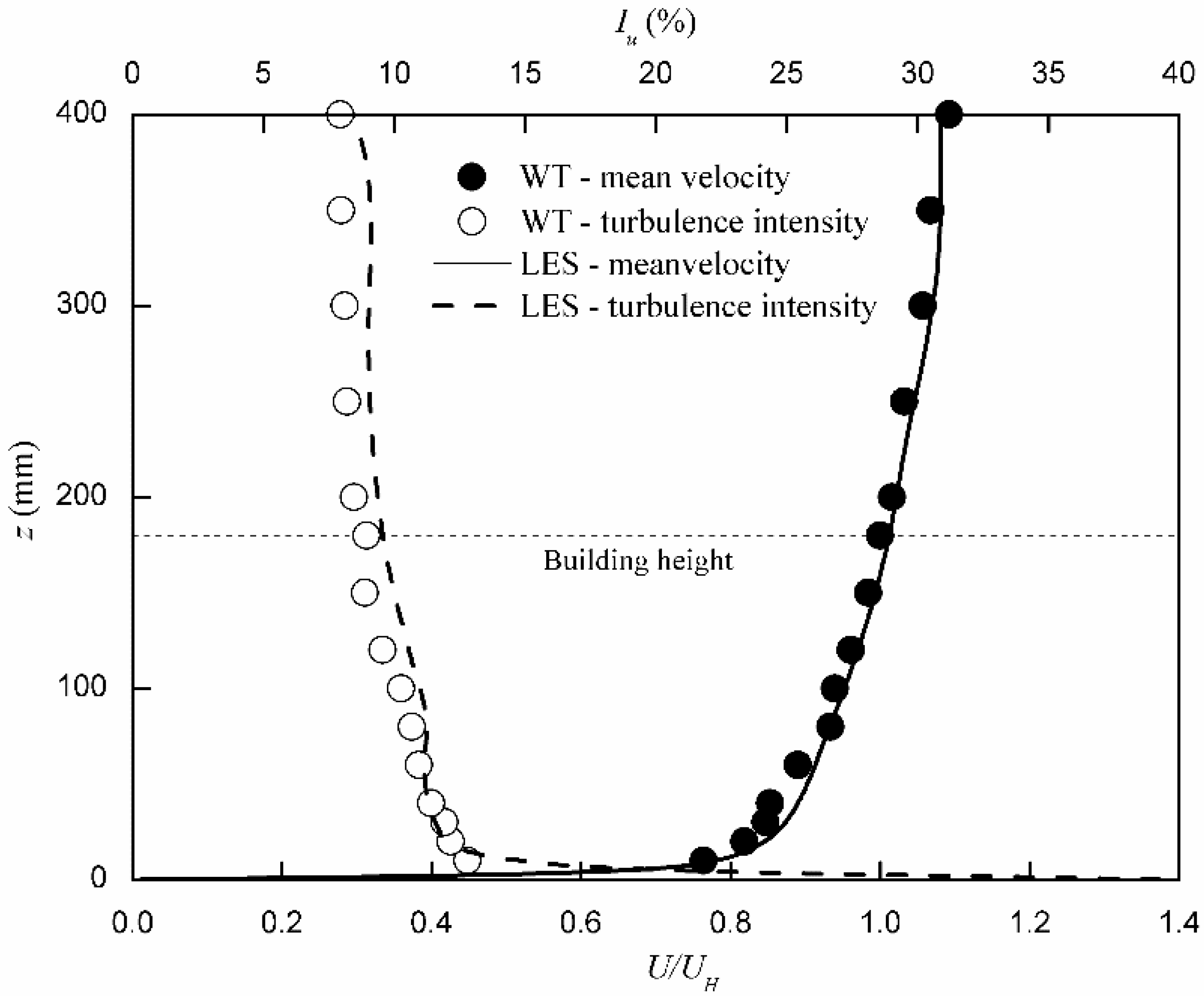
Figure 4.
Layout of pressure taps on principal building model (unit: mm).
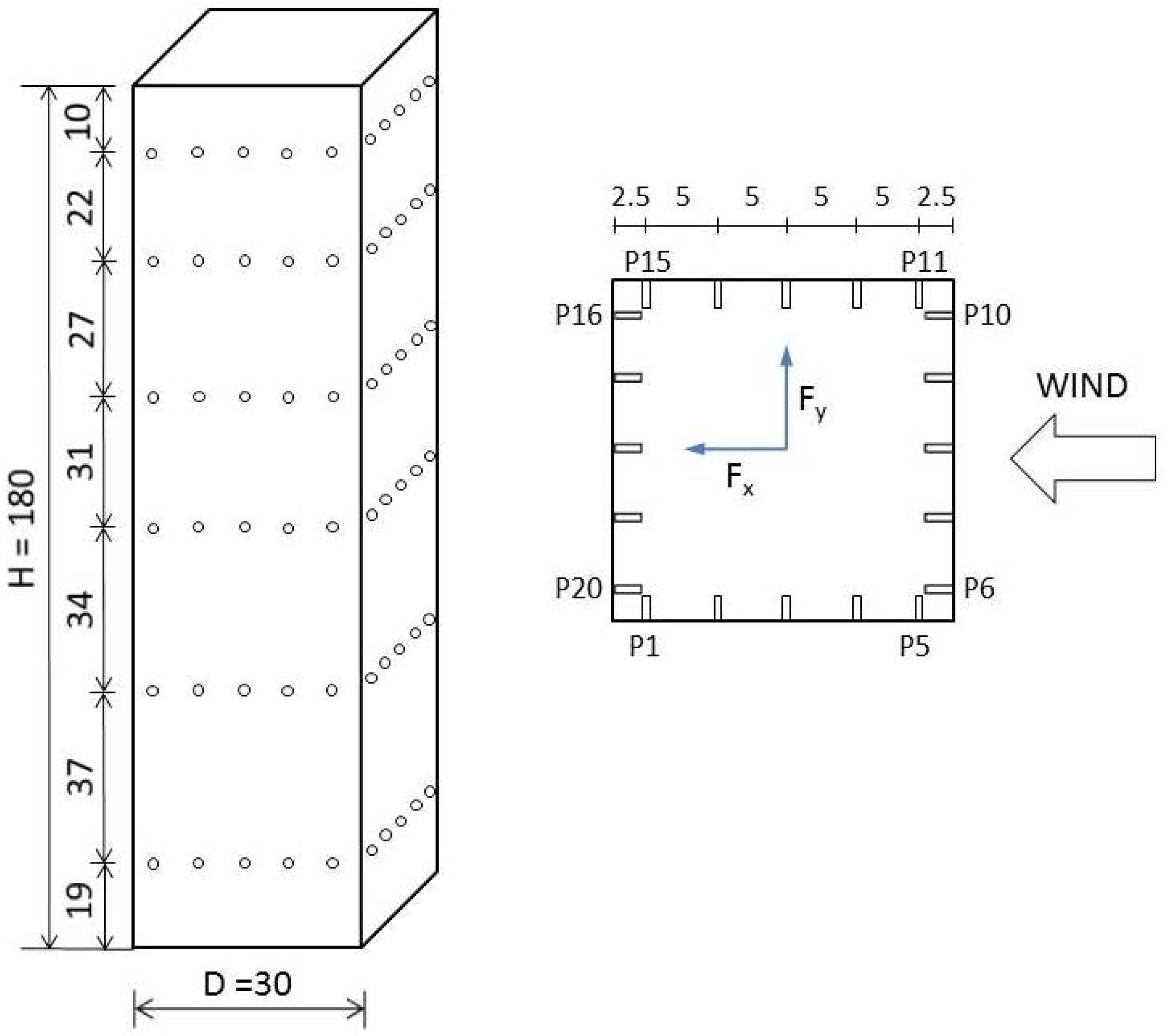
Figure 5.
PIV set-up in wind tunnel.

Figure 6.
Wind velocity field for normal wind incidence. (a) Time-averaged mean flow field; (b) RMS flow field.
Figure 6.
Wind velocity field for normal wind incidence. (a) Time-averaged mean flow field; (b) RMS flow field.

Figure 7.
Time-averaged streamlines at mid-height: (a) LES result and (b) wind tunnel result.
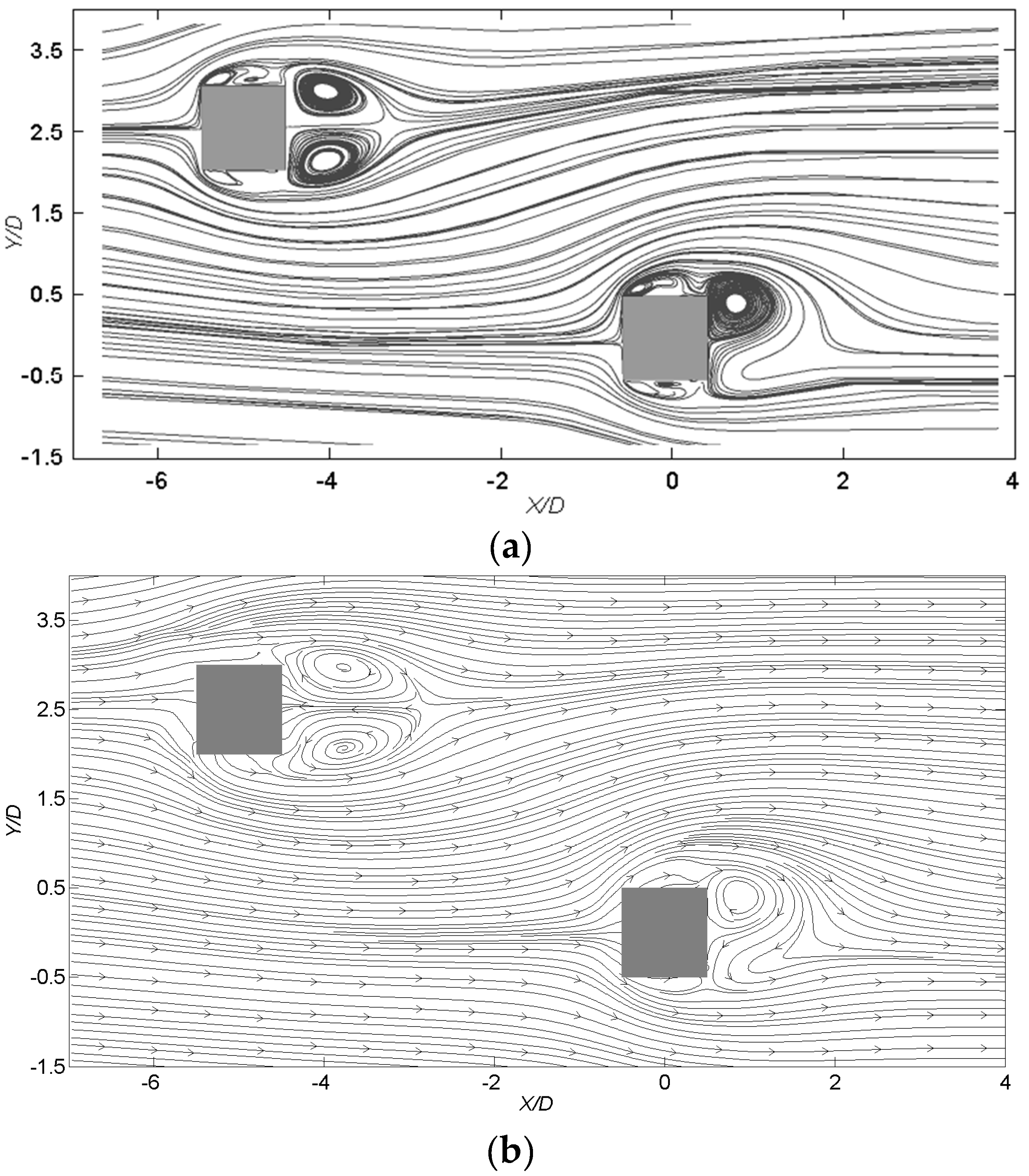
Figure 8.
Comparison of wind tunnel (WT) measurements and LES results of mean streamwise velocity in horizontal plane: (a) Level 3 (h = 0.5H) and (b) Level 5 (h = 0.82H). Wind velocity plots transversely with positive value on right side of the dotted axis and negative on left side.
Figure 8.
Comparison of wind tunnel (WT) measurements and LES results of mean streamwise velocity in horizontal plane: (a) Level 3 (h = 0.5H) and (b) Level 5 (h = 0.82H). Wind velocity plots transversely with positive value on right side of the dotted axis and negative on left side.

Figure 9.
Comparison of wind tunnel (WT) measurements and LES results of mean transverse velocity in horizontal plane: (a) Level 3 (h = 0.5H) and (b) Level 5 (h = 0.82H). Wind velocity plots transversely with positive value on right side of the dotted axis and negative on left side.
Figure 9.
Comparison of wind tunnel (WT) measurements and LES results of mean transverse velocity in horizontal plane: (a) Level 3 (h = 0.5H) and (b) Level 5 (h = 0.82H). Wind velocity plots transversely with positive value on right side of the dotted axis and negative on left side.

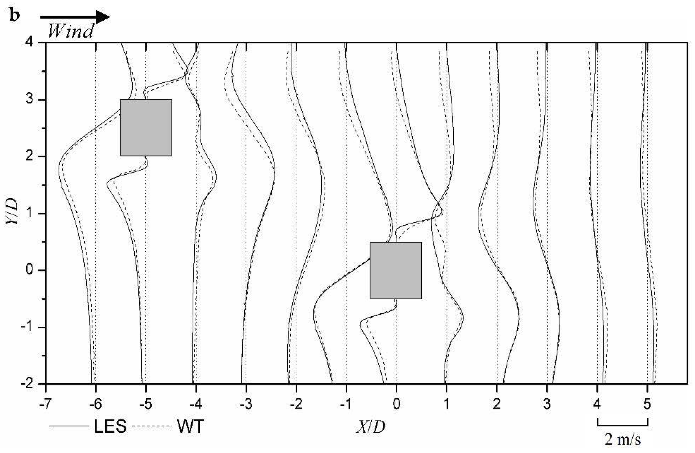
Figure 10.
Comparison of wind tunnel (WT) measurements and LES results of fluctuating streamwise velocity u’ in horizontal plane: (a) Level 3 (h = 0.5H) and (b) Level 5 (h = 0.82H). Wind velocity plots transversely with positive value on right side of the dotted axis and negative on left side.
Figure 10.
Comparison of wind tunnel (WT) measurements and LES results of fluctuating streamwise velocity u’ in horizontal plane: (a) Level 3 (h = 0.5H) and (b) Level 5 (h = 0.82H). Wind velocity plots transversely with positive value on right side of the dotted axis and negative on left side.

Figure 11.
Comparison of wind tunnel (WT) measurements and LES results of fluctuating transverse velocity v’ in horizontal plane: (a) Level 3 (h = 0.5H) and (b) Level 5 (h = 0.82H). Wind velocity plots transversely with positive value on right side of the dotted axis and negative on left side.
Figure 11.
Comparison of wind tunnel (WT) measurements and LES results of fluctuating transverse velocity v’ in horizontal plane: (a) Level 3 (h = 0.5H) and (b) Level 5 (h = 0.82H). Wind velocity plots transversely with positive value on right side of the dotted axis and negative on left side.

Figure 12.
Normalized spectrum of across-wind forces on different levels along building height.

Figure 13.
Conditionally sampled wind velocity field at: (a) peak maximum across-wind forces (g = 2) and (b) peak minimum across-wind forces (g = −2).
Figure 13.
Conditionally sampled wind velocity field at: (a) peak maximum across-wind forces (g = 2) and (b) peak minimum across-wind forces (g = −2).
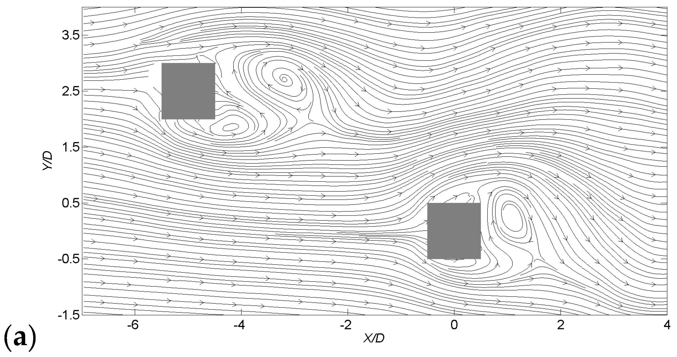
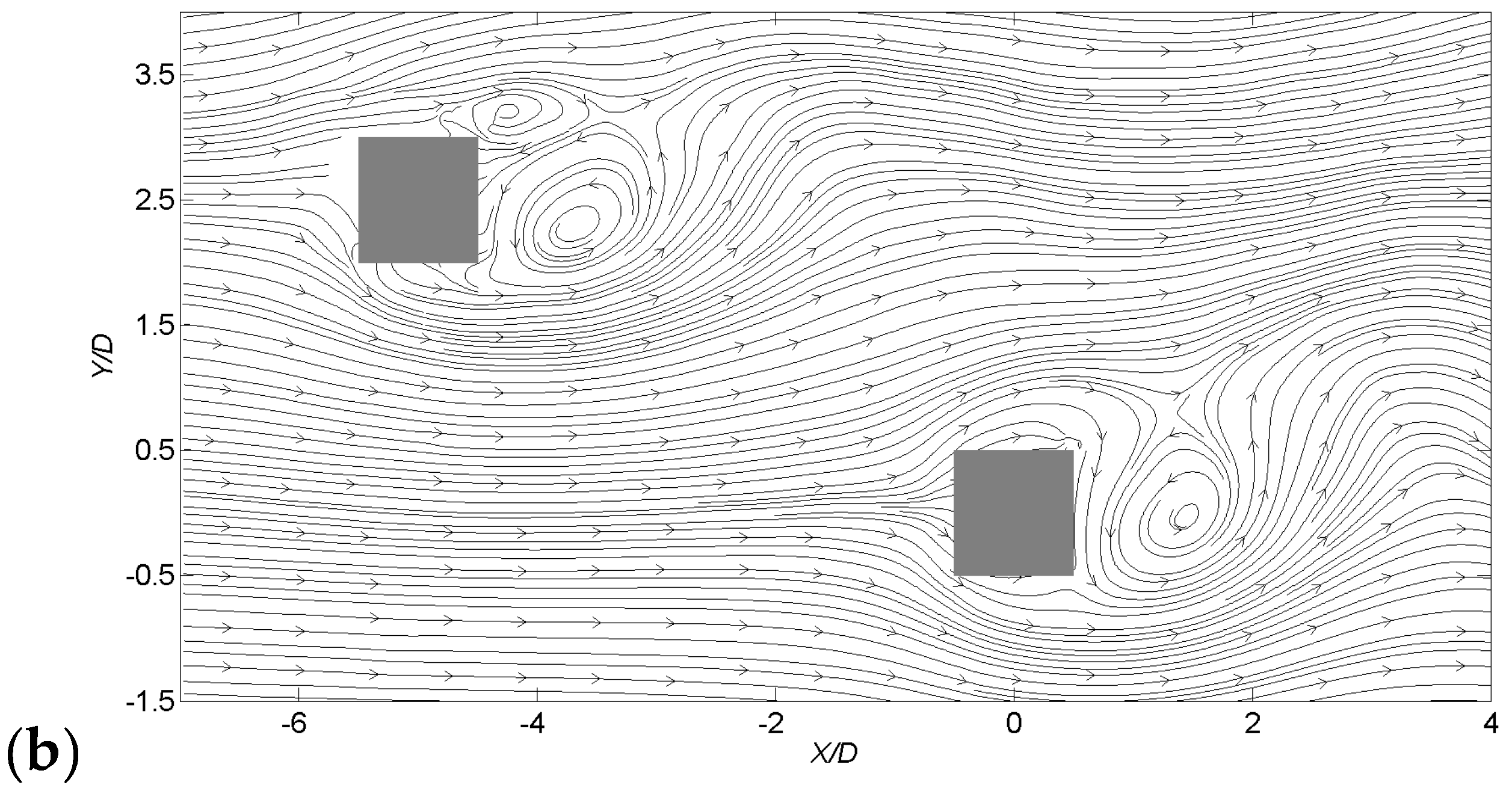
Figure 14.
Three-dimensional view of Instantaneous vortex structures represented by spanwise vorticity ω* = ωD/U: (a–c) positive across-wind force (upward) event and (d–f) negative across-wind force (downward) event; (a,d) Iso-surfaces of ω* = −2~−5; (b,e) Iso-surfaces of ω* = 2~5; (c,f) Vector field at mid-height.
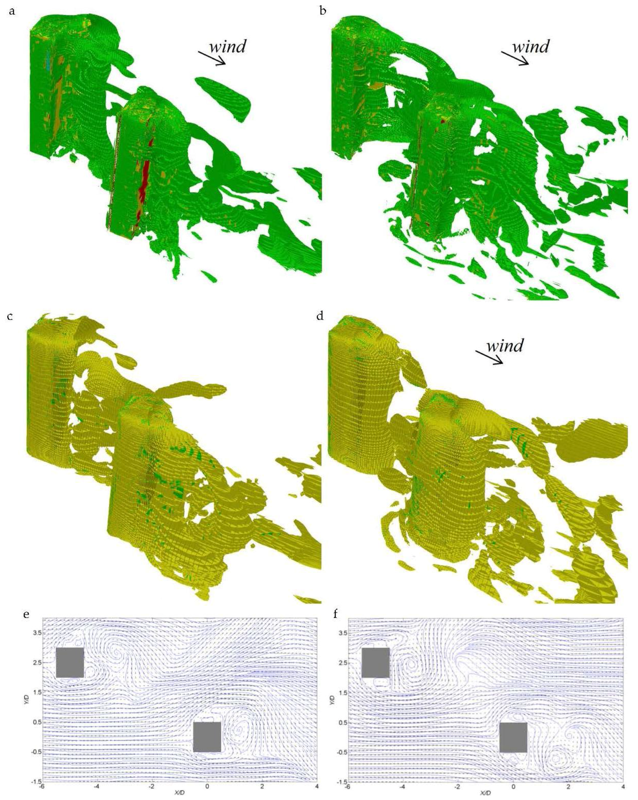
Figure 15.
Local across-wind force coefficients obtained from LES and wind tunnel tests.
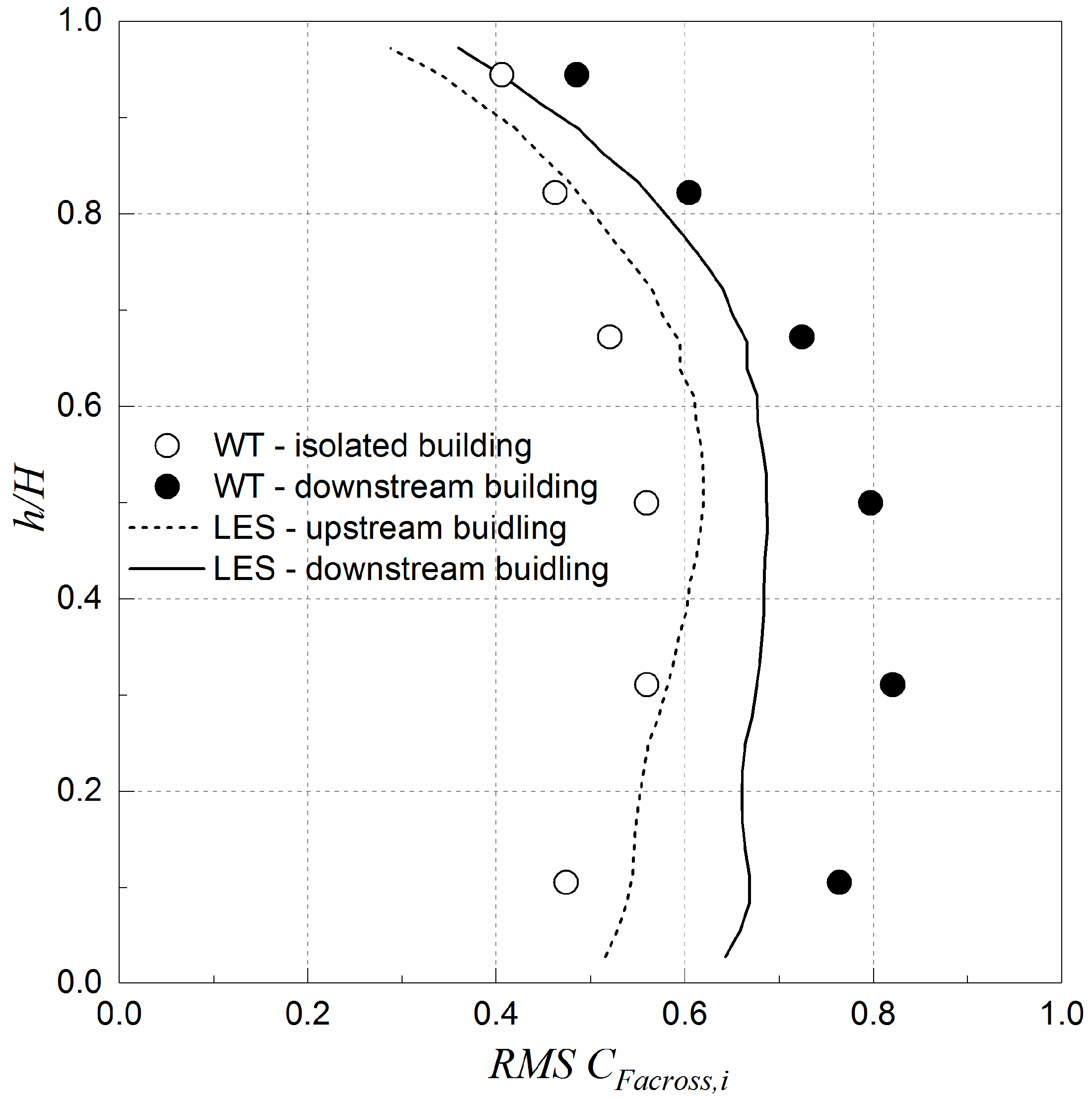
Figure 16.
Simultaneous fluctuating overall across-wind force coefficients on upstream building and downstream building.
Figure 16.
Simultaneous fluctuating overall across-wind force coefficients on upstream building and downstream building.
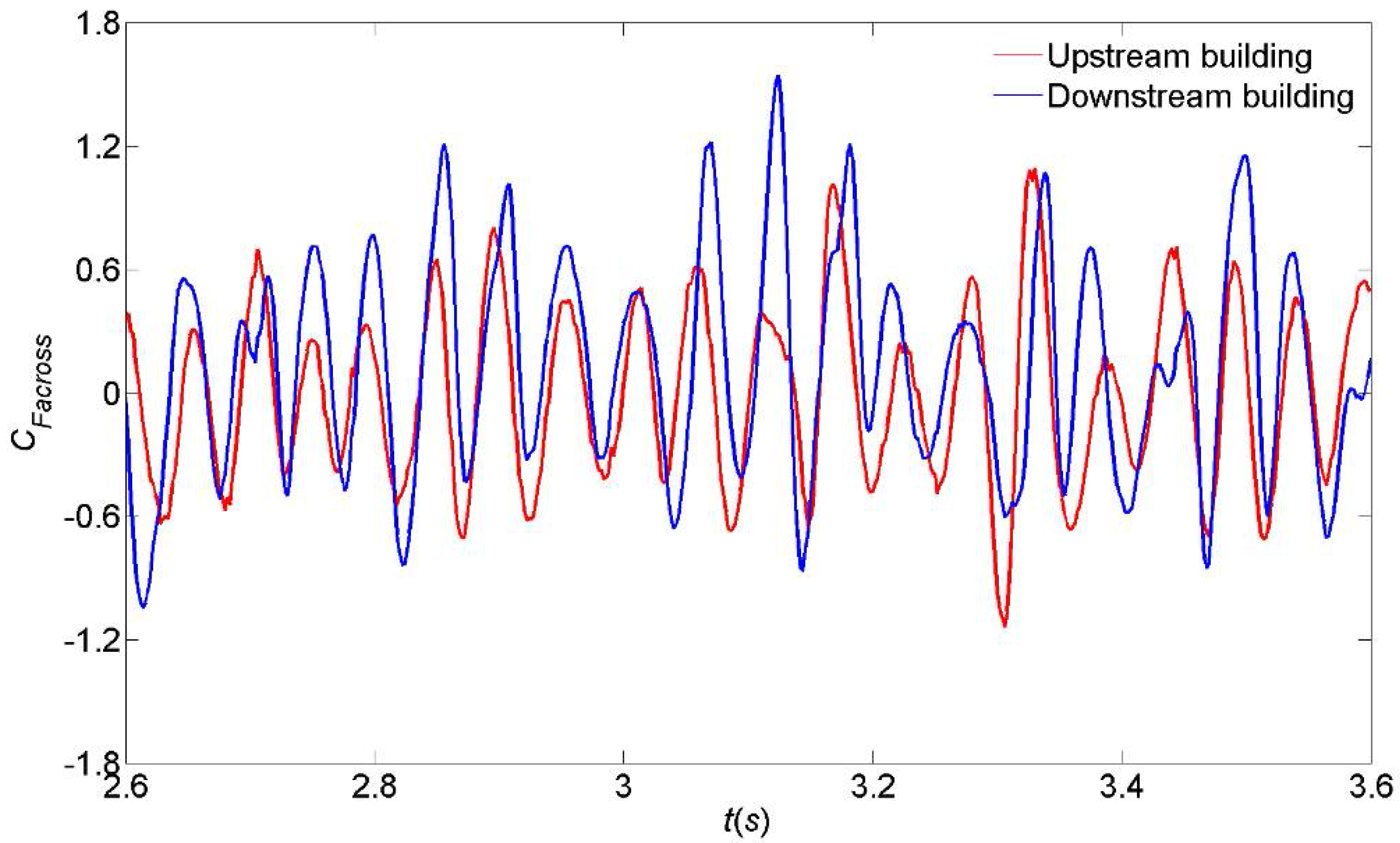
Figure 17.
Simultaneous fluctuating surface pressure coefficient Cross correlation curves between across-wind forces on upstream building and downstream building.
Figure 17.
Simultaneous fluctuating surface pressure coefficient Cross correlation curves between across-wind forces on upstream building and downstream building.
© 2018 by the authors. Licensee MDPI, Basel, Switzerland. This article is an open access article distributed under the terms and conditions of the Creative Commons Attribution (CC BY) license (http://creativecommons.org/licenses/by/4.0/).
Share and Cite
MDPI and ACS Style
Zu, G.; Lam, K.M. LES and Wind Tunnel Test of Flow around Two Tall Buildings in Staggered Arrangement. Computation 2018, 6, 28. https://doi.org/10.3390/computation6020028
AMA Style
Zu G, Lam KM. LES and Wind Tunnel Test of Flow around Two Tall Buildings in Staggered Arrangement. Computation. 2018; 6(2):28. https://doi.org/10.3390/computation6020028
Chicago/Turabian StyleZu, Gongbo, and Kit Ming Lam. 2018. "LES and Wind Tunnel Test of Flow around Two Tall Buildings in Staggered Arrangement" Computation 6, no. 2: 28. https://doi.org/10.3390/computation6020028
Note that from the first issue of 2016, this journal uses article numbers instead of page numbers. See further details here.