Analyzing the Effect and Performance of Lossy Compression on Aeroacoustic Simulation of Gas Injector

Abstract

Computational fluid dynamic simulations involve large state data, leading to performance degradation due to data transfer times, while requiring large disk space. To alleviate the situation, an adaptive lossy compression algorithm has been developed, which is based on regions of interest. This algorithm uses prediction-based compression and exploits the temporal coherence between subsequent simulation frames. The difference between the actual value and the predicted value is adaptively quantized and encoded. The adaptation is in line with user requirements, that consist of the acceptable inaccuracy, the regions of interest and the required compression throughput. The data compression algorithm was evaluated with simulation data obtained by the discontinuous Galerkin spectral element method. We analyzed the performance, compression ratio and inaccuracy introduced by the lossy compression algorithm. The post processing analysis shows high compression ratios, with reasonable quantization errors.

1. Introduction

Nowadays, with the high availability of computing power, simulation methods have evolved into important tools in many research areas and industry. Current supercomputers such as the Cray XC40 (Hazel Hen) have on the order of ${10}^5$–${10}^6$ computing cores and peak performances of multiple Pflop/s [1]. Many application areas, such as computational fluid dynamics (CFD), have benefited greatly from the massive increase of computing power over the past decades, by specifically developing and implementing parallel codes [2]. On the basis of these codes, it is possible to carry out detailed studies of complex fluid mechanics phenomena, such as turbulent boundary layer effects of a supersonic flow [3] or the flow in the turbine of a helicopter [4]. To ensure that all the relevant characteristics of such complex fluid flow simulations are captured correctly, the simulation domain needs to be discretized with high resolution. Information such as density, momentum and the specific total energy needs to be stored for every discretization point, e.g., in a parallel file system. The combination of huge simulation domains and high temporal and spatial resolution leads to terabytes of simulation results, e.g., for the simulation of the fluid flow in the turbine of a helicopter [4]. This leads to new challenges for high-performance computing. The available bandwidth to the file system is a limiting factor for CFD simulations and can lead to massive performance degradation. In the future, this problem will most likely become even bigger, as it is reasonable to assume that the increase in computing power will be faster than the increase in available I/O-bandwidth. Furthermore, the time to communicate data within the simulation increases, with the increasing amount of data to be communicated.

The large amounts of data are not only a challenge during the simulation, it is also a challenge for post-processing. To analyze and visualize the simulation results, data needs to be accessed from the file system, and again I/O-bandwidth is a limiting factor. Furthermore, archiving the simulation results in itself is a challenge and often, the data has to be stored for years. All these problems scale with the size of data, therefore, the most straight forward remedy is to reduce the amount of data. One way to achieve this would be to reduce the temporal and spatial resolution. However, a reduction of the resolution heavily impacts the accuracy of the results. An alternative is to use data compression techniques. Data compression can be divided in two main categories, lossless or lossy. lossless data compression has more acceptance in scientific field but the compression ratio is limited. In order to increase the compression ratio, Burtscher et al. employed genetic algorithm to find an effective lossless compression algorithm during runtime. To achieve this, they have selected the basic elements that are typically used in compression algorithms and can be implemented to run in linear time. During the runtime they search for the most effective chain of the basic elements [5]. A higher compression ratio can also be obtained by lossy data compression algorithms. Recently, several studies have been analyzing the effects of lossy data compression algorithms in scientific simulations [6,7,8]. Laney et al. show that the lossy compression is suitable in simulations. Their evaluation method is more realistic due to the observation of physic based metrics other than classical error metrics [7]. Baker et al. show that applying lossy data compression to climate simulation data is both advantageous in terms of data reduction and acceptable in terms of effects on scientific results. They provided both lossy and original data, and challenged climate scientists to examine features of the data relevant to their interests and identify which of the ensemble members have been compressed and reconstructed [8].

In this work, an efficient online lossy compression framework of floating point simulation data is presented, and the effect and performance of lossy compression is analyzed on aeroacoustic simulation data of gas injectors. The presented compression framework provides a capability of dynamically selecting a suitable compression algorithm and also exploiting spatially adaptive quantization to get better compression ratio while still satisfying a maximum relative error tolerance.

Simulation Method

The CFD code used in this work is based on the discontinuous Galerkin spectral element method (DG SEM). The method is well described in the literature, so we restrict ourselves to a short overview of DG SEM. For further reading we refer to [2]. Starting point of DG SEM are the compressible Navier–Stokes equations expressed in conservative form:

$${\mathit{u}}_t\left(\mathit{x}\right)+{\mathbf{\nabla }}_x·\mathit{F}(\mathit{u}\left(\mathit{x}\right),{\mathbf{\nabla }}_x\mathit{u}\left(\mathit{x}\right))=\mathbf{0}\forall \mathit{x}\in \Omega .$$

(1)

where $\mathit{F}$ contains the physical fluxes, $\Omega$ is the computational domain, and $\mathit{u}$ is a vector containing the conservative variables that is given by:

$$\mathit{u}=\left(\begin{array}{c}\rho \\ \rho {\upsilon }_1\\ \rho {\upsilon }_2\\ \rho {\upsilon }_3\\ \rho e\end{array}\right).$$

(2)

The conservative variables are the density, momentum, and the specific total energy. The simulation domain is divided into hexahedral grid cells. Each grid cell is mapped to the reference element $E={[-1,1]}^3$ with coordinates $\mathit{\xi }={({\xi }^1,{\xi }^2,{\xi }^3)}^T$. The actual computation is performed in the reference element and integrated over the reference element, to get the so-called weak formulation. To derive the discontinuous Galerkin (DG) formulation, the transformed conservative law is multiplied with a test function $\Phi$. The solution in each reference element is approximated by tensor products of Lagrangian polynomials of degree N:

$$\mathit{u}\left(\mathit{\xi }\right)=\sum _{i.j.k=0}^N{\widehat{\mathit{u}}}_{\mathit{i},\mathit{j},\mathit{k}}{\psi }_{i,j,k}\left(\mathit{\xi }\right)\mathrm{with}{\psi }_{i,j,k}\left(\mathit{\xi }\right)=l_i\left({\xi }^1\right)l_j\left({\xi }^2\right)l_k\left({\xi }^3\right),$$

(3)

where $\widehat{u_{i,j,k}}:=\widehat{u_{i,j,k}}\left(t\right)$ are the time dependent degrees of freedom (DOFs), and $l_i\left(\xi \right)$ are the Lagrange interpolation polynomials defined by a nodal set ${\left\{{\xi }_i\right\}}_{i=0}^N$. Each element has ${(N+1)}^3$ nodes, each node contains the five conservative variables. DG schemes are a hybrid of Finite Element schemes and Finite Volume schemes. The solution is approximated by an element-local polynomial basis and the solution is discontinues over element boundaries. This denotes that adjacent elements have different states at the interface. Adjacent elements are coupled by fluxes through their interfaces. For the approximation of the boundary flux ${\mathcal{F}}^{*}$, a Riemann solver is used with the information form the state $\mathit{u}$ of an element and the state ${\mathit{u}}^{+}$ of the neighboring element. In the present study, we use the local Lay–Friedrich method [9]. The integration in the DG discretization is solved by Gauss quadrature. The time integration is done with an explicit 3rd-order accurate Runge-Kutta scheme.

2. Related Work

There are several works involving compression of CFD simulation data [10,11,12,13,14,15]. Wavelet-based compression algorithms is one of the most common techniques used. Sakai et al. proposed a lossy compression method using discrete wavelet transform (DWT) followed by quantization and entropy encoding [12,13,14,15]. The main drawback of their approach is that there is no straightway to control the amount of the compression error. However, in this work the accuracy is guaranteed to stay within a certain threshold. Additionally, wavelet transforms produce noise near the rapid signal transition. Therefore, it is not suitable for our simulation data which are generated through the discontinuous Galerkin spectral element method, due to the discontinuities between the neighboring elements. In another work the usefulness of image and video compression technique for compressing CFD data on regular Cartesian grids was investigated [10]. They have compared three main compression algorithms in that domain namely JPEG, JPEG-2000, and MPEG. It was found that JPEG-2000 requires a lot of computing time, mainly because of the wavelet transform, the MPEG compressor requires the input data to be scaled from double floating point to an integer array [0,255], which is time consuming and leads to a very high maximum error of approx. 10% and the main drawback of JPEG compression is that the decompression step takes a lot of time, while giving no possibility to control the generated error on individual data points. Tensor decompositions are another method that is used for compressing multi-dimensional array by reducing the dimension of input data set. This method can provide higher compression ratio than the wavelet transforms or discrete cosine transform (DCT) [16]. However, it cannot guarantee point wise error bound which is the main constraint of this work. Additionally, this method is suffering from computation time but this can be improved by parallel implementation. Austin et al. enhanced the performance by parallelizing the method, and overlapping communication and computation on a Cray XC30 supercomputer [17].

There are several works that support point-wise user defined error bound based on subsequent analysis requirements [18,19,20,21]. Iverson et al. investigated a method for grid-based scientific data set. In the proposed approach the value of set of nodes are replaced by a constant value that satisfies the reconstruction error bound, followed by a lossless compression [19]. In comparison to this work they bound the absolute error and not the relative error. Another lossy compression algorithm is ISABELA [18,22], which utilizes B-Splines to approximate the values in the data stream. It divides the continuous stream of floating point numbers into windows of an user-defined length, and then sorts the numbers in every window. This sorting reduces random fluctuations and provides a smoother, monotonically increasing sequence, which is then approximated by a B-Spline. In order to ensure a specific point to point error, the difference between the approximation and the real value is stored in a quantized integer. FPZIP is another compression algorithm that is based on predictive coding and uses three dimensional Lorenzo predictor followed by residual computation and a fast entropy encoder [20,23]. Another algorithm is ZFP [24], which focused on compression of 3D arrays of floating point numbers. The compression algorithm consists of three main steps: conversion to fixed-point, an orthogonal block transform and bit plane encoding. One of the main advantages of ZFP is efficient random-access reads and writes, which is not available in other lossy floating point data compression algorithm. The last compression algorithm that is used for comparison is applying a Lorenzo predictor that exploits the spatial correlation [25]. Three different dimension of Lorenzo predictor is used for comparison by replacing them with the predictor that is used in this work and keeping all other component unchanged. The detailed comparison with the mentioned work is given in Section 5.4.

In this work, a prediction-based compression algorithm is used that exploits the temporal coherence between subsequent simulation frames. The main drawback of this method is that it is not possible to access any time step randomly. It means that to access any of the time step for post processing analysis, all earlier time steps must be decompressed first. Nevertheless, most of the time these data are used for 3D visualization where complete data sets are read sequentially every time some viewing parameter is changed. In such a case the presented method would provide no drawbacks. Another drawback of prediction-based method is that, there should be sufficient memory to buffer one simulation time step. However in our test case each simulation time steps is less than 1 Gbyte. Which is in an acceptable range. For the Cray XC40 (Hazel Hen) supercomputer, each node has 128 Gbyte of memory. Hence the authors feel that the memory problem to buffer only a single time step would not be a major bottleneck in many cases.

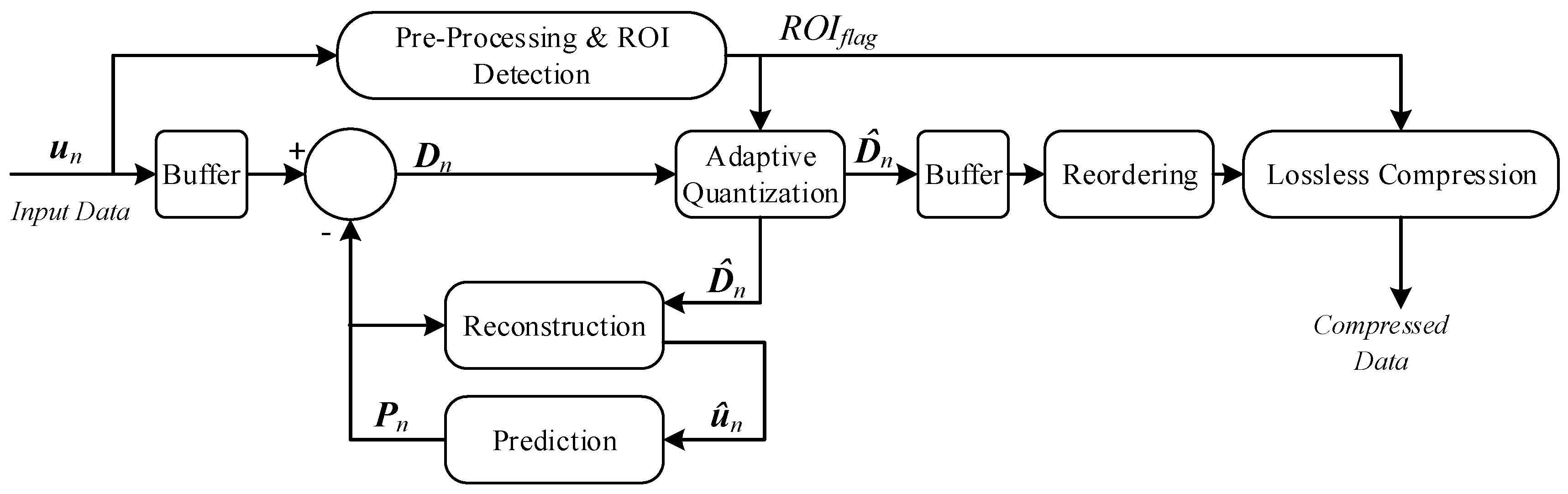
3. Data Compression Method

In order to compress the CFD data, a prediction based compression algorithm is applied [26]. The compression is performed on all conservative variables. As it is shown in Figure 1 the compression algorithm consists of four main parts, region of interest (ROI) detection, prediction module, quantization module and lossless compression algorithm module. These parts are explained in the following subsections.

3.1. Pre-Processing and ROI Detection

The main purpose of the region of interest scheme is that all the simulation data are not equally important for the post processing or visualization phase. Therefore, the goal is to detect and identify more relevant regions and compress them with a smaller quantization level to achieve higher decompressed data quality. Those regions can be identified by various criteria such as their position or by the value of specific quantities such as temperature, pressure or turbulence.

In this work, for the investigated simulation case, i.e., natural gas injector, the temperature is a suitable indicator for the ROI. Flow phenomena such as pressure shocks or strong turbulence directly influence the temperature. For instance, Figure 2a shows a snapshot of the temperature of the external flow behind an injector, more specific details about the injector is given in Section 4. Figure 2b shows the ROI that is based on the temperature value, and in this example the ROI is where the temperature value (T) is higher than 300 K. Figure 2c shows the ROI that is based on the position of the simulation elements and was defined before the simulation has started. Figure 2d is the combination of the two previous examples. Figure 2e shows the ROI that is based on the temperature value, and in this example the ROI is where the temperature value (T) is lower than 300 K. There are no implicit advantages or disadvantages between the different ROI. Rather, the ROI should match the actual use case. For instance, Figure 2e is used for sound pressure level analysis, as the observation points are in the region with almost no turbulence which are cooler than the turbulent regions. More detailed information about the ROI is given in Section 5.

For each DG-element one $RO{I}_{flag}$ is defined, where $RO{I}_{flag}$ is True if one or more nodes in the DG-element satisfy the ROI condition. Hence, only one bit per DG-element is the overhead of the ROI technique, and the process of detecting ROI DG-elements is stopped as soon as the first node in the DG-element satisfies the ROI condition.

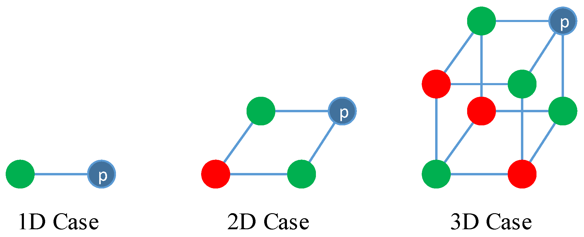
3.2. Prediction and Reconstruction

By taking advantage of the prediction based algorithm, the variance and dynamic range of the data is be reduced. The amount of the reduction depends on how well the predictor can predict the next value. In this work, a very simple but fast and effective polynomial predictor is used [27]. The prediction is defined as:

$${\mathit{P}}_{\mathit{t}}={\widehat{\mathit{u}}}_{\mathit{t}-\mathbf{1}},$$

(4)

where ${\widehat{\mathit{u}}}_{\mathit{t}-\mathbf{1}}$ is the reconstructed value of the previous simulation time step. The predictor in the compression unit should use the same data that the predictor in the decompression unit will use. Therefore, due to the quantization and lossy compression, the compressed data must be reconstructed in the compression unit. The reconstructed value is derived by:

$${\widehat{\mathit{u}}}_{\mathit{t}}={\mathit{P}}_t+{\widehat{\mathit{D}}}_{\mathit{t}}\times \mathbf{\Delta },$$

(5)

where $\mathbf{\Delta }$ is the quantization step vector, and ${\widehat{\mathit{D}}}_{\mathit{t}}$ is the quantized values of prediction residuals. These two values are explained in the following section.

3.3. Adaptive Quantization

The prediction residual of the polynomial predictor is defined as:

$${\mathit{D}}_{\mathit{t}}={\mathit{u}}_{\mathit{t}}-{\mathit{P}}_t,$$

(6)

which is a floating point variable. By this step the prediction residual, $D_t$, is converted to an integer. This conversion is done by division of the input amplitude by a quantization step size, $\Delta$, followed by rounding to the nearest integer and is expressed as follows:

$${\widehat{\mathit{D}}}_{\mathit{t}}=\mathrm{round}(\frac{{\mathit{D}}_{\mathit{t}}}{\mathbf{\Delta }}).$$

(7)

The quantization is the only source of loss of precision: a small $\mathbf{\Delta }$ will lead to a higher precision but reduces the compression ratio. Accordingly, $\mathbf{\Delta }$ has a direct relation both with the compression ratio and the loss of precision. In this work, the value of the $\mathbf{\Delta }$ is a unique value for each conservative variable in each DG-element, and depends on the requested permissible maximum relative error (PMRE) for ROI and non-ROI regions. With this approach the accuracy is guaranteed to stay within PMRE.

In order to calculate the $\Delta$ we need to define the following: Let us assume that the original value $\mathit{A}$ is a vector of size m, $\mathit{A}=\{a_0,a_1,...,a_{m-1}\}$, the reconstructed value $\widehat{\mathit{A}}$ is respectively $\widehat{\mathit{A}}=\{{\widehat{a}}_0,{\widehat{a}}_1,...,{\widehat{a}}_{m-1}\}$, and $I=\{0,1,...,m-1\}$. In this work m is the number of nodes in one DG-element. Suppose that maximum absolute error ($\mid e{\mid }_{max}$) and maximum relative error (MRE) due to the quantization are defined as following:

$$\begin{array}{cc}\hfill \mid e{\mid }_{max}& =\underset{i\in I}{max}|a_i-{\widehat{a}}_i|\hfill \\ & \le \frac{\mathbf{\Delta }}{2},\hfill \end{array}$$

(8)

and:

$$\begin{array}{cc}\hfill MRE& =\underset{i\in I}{max}\left|\frac{a_i-{\widehat{a}}_i}{a_i}\right|\hfill \\ & \le \frac{\mid e{\mid }_{max}}{\mid \mathit{A}{\mid }_{min}}\hfill \\ & \le \frac{\mathbf{\Delta }}{2\times \mid \mathit{A}{\mid }_{min}}.\hfill \end{array}$$

(9)

We have defined $PMRE$ to be an upper bound for $MRE$. Therefore, from Equation (9) and by assuming two different values for $PMRE$ at ROI and non-ROI region, namely $PMR{E}_{ROI}$ and $PMR{E}_{non-ROI}$, the quantization step size is calculated as follows:

$$\mathbf{\Delta }=\left\{\begin{array}{cc}2\times PMR{E}_{ROI}\times \mid \mathit{A}{\mid }_{min},\hfill & \mathrm{if}RO{I}_{flag}=1\hfill \\ 2\times PMR{E}_{non-ROI}\times \mid \mathit{A}{\mid }_{min},\hfill & \mathrm{if}RO{I}_{flag}=0.\hfill \end{array}\right.$$

(10)

The only unknown variable in Equation (10) is $\mid \mathit{A}{\mid }_{min}$, which must be calculated for each conservative quantity in each DG-element, and should be transferred to the output stream. Afterward, the decoder can derive the $\mathbf{\Delta }$ by extracting $\mid \mathit{A}{\mid }_{min}$, $RO{I}_{flag}$, $PMR{E}_{ROI}$, and $PMR{E}_{non-ROI}$ from the compressed stream. In case of overflow or division by zero in Equation (9), no quantization is performed on that specific DG-elements.

3.4. Reordering and Lossless Compression

The last chain of the compression algorithm is a lossless compression algorithm that exploits all repetition in the data and achieve a higher compression ratio by representing frequently occurring patterns with few bits and rarely occurring patterns with many bits [28,29,30]. Additionally, in order to gain a higher compression ratio, the residual of the conservative variables are reordered. It means that the residuals of each conservative quantity are grouped together and then are passed to the lossless compression module.

4. Adaptive Compression Framework

In the context of scientific simulation data compression, traditionally, a single compression algorithm is used, which is selected independently from the environment parameters. However, a fixed compression algorithm prevents dynamic adjustments to changes in the data distribution, data properties or external factors. Therefore, an adaptive compression framework is introduced, which utilizes different compression algorithms, in order to dynamically adjust the compression process to specific conditions. The main task is the adaption to the availability of computing resources, particular the network environments. If the current bandwidth in the network drops, it may be beneficial to change the current compression to an algorithm which achieves better compression ratios at a lower throughput, in order to reduce the overall transmission time of the data in the network.

In order to allow for adaptive compression, the data is divided into multiple windows and each window is divided further into multiple frames. In this work, one frame consists of 100 DG elements. As it is shown in Figure 3, the functionality of the framework can be divided into the three following parts. First, the so called modules, which represents a single algorithm in the compression framework and provide an encoding and decoding function for that algorithm. These modules can be chained together and behave like a pipeline, which allows an implementation of different compression pipelines or even the implementation of an adaptive compression scheme, in which the individual modules are selected at run time. In this work, there are five main modules. Module A (prediction and quantization module) and Module B (reordering module) are fixed for all frames in the compression pipeline and won’t change during runtime. However, Modules C, D and E, which are the lossless compression algorithms , may be alternate during runtime. This means that frames can be compressed with different lossless compression algorithms. For instance, by considering that each window has 20 frames, the first 10 frames can be encoded by Module C, while the next nine consecutive frames are encoded by Module D and the last frame is encoded by Module E. The second part is a central monitoring component, which is used to store performance records for every compressed frame, and make these records accessible to the framework. The stored records contain aggregated information over the whole compression, as well as detailed information about the achieved compression ratio and run time duration of each individual module, which was used to compress the corresponding data. The last part of the framework is the central decision unit, which selects the modules, used for the current window. Its strategy is implemented by the user and can range from a simple selection of the same compression modules for each frame in the window, to complex strategies based on information provided by the monitoring component and external information.

In the next section we describe how to choose the most suitable configuration of different encoding algorithms during run time.

Optimization

The objective of the optimization is to find a proper decision policy with respect to the optimization goals. A goal can be to maximize the total compression ratio ($C_{total}$) given restrictions on computing time and network bandwidth. Thus, the total output rate ($R_{total}$) should be slightly higher than the available network throughput ($T{R}_{av}$). This goal can be formulated as:

$$max\left\{C_{total}\right|R_{total}>T{R}_{av}\}.$$

(11)

The optimization process is done only once at the beginning, and the decision unit will use the results of the optimization process during run time. To achieve a more adaptive behavior the optimization process can of course be repeated during run time at the cost of computation time.

In order to adjust the output rate, the decision unit changes the ratio between the amount of lossless compression algorithms invocations during run time. Therefore, we define a window size, which represents the number of subsequent frames, for which the output rate of the compression is adjusted. A fraction of those frames in the window is then compressed with different lossless compression algorithms. Therefore window size can be defined as

$$\begin{array}{c}\hfill WindowSize=\sum _{i=1}^n{x}_i,\end{array}$$

(12)

where $x_i$ is the number of invocations of the i-th lossless compression algorithm, and n is the number of the lossless compression algorithms. For every lossless compression algorithm we have defined the output rate as:

$$R_i=\frac{C{S}_i}{t_i},$$

(13)

and the compression ratio obtained by the i-th lossless compression algorithm as:

$$C_i=\frac{DS}{C{S}_i},$$

(14)

where $C{S}_i$ is the size of the compressed data obtained by the i-th lossless compression algorithm, $DS$ is the size of one frame, and $t_i$ is the required time to compress one frame. Since the data that are in subsequent frames are very similar, it is assumed that every lossless compression algorithms achieves an almost identical compression ratio and output rate for subsequent frames. The validity of this assumption is proven experimentally in Section 5.4. By considering this assumption the total compression ratio in a window is given by:

$$\begin{array}{cc}\hfill C_{total}& =\frac{WindowSize\times DS}{{\displaystyle \sum _{i=1}^n}{x}_i\times C{S}_i}\hfill \\ & =\frac{WindowSize}{{\displaystyle \sum _{i=1}^n}{x}_i/C_i},\hfill \end{array}$$

(15)

and the total output rate of a window can be calculated from:

$$\begin{array}{cc}\hfill R_{total}& =\frac{x_1\times C{S}_1+x_2\times C{S}_2+...+x_n\times C{S}_n}{x_1\times t_1+x_2\times t_2+...+x_n\times t_n}\hfill \\ & =\frac{{\displaystyle \sum _{i=1}^n}(x_i\times C{S}_i)}{{\displaystyle \sum _{i=1}^n}(x_i\times t_i)}.\hfill \end{array}$$

(16)

From Equations (13), (14) and (16), we have:

$$\begin{array}{cc}\hfill R_{total}& =\frac{{\displaystyle \sum _{i=1}^n}(x_i\times DS/C_i)}{{\displaystyle \sum _{i=1}^n}(x_i\times (DS/(C_i\times R_i))}\hfill \\ & =\frac{{\displaystyle \sum _{i=1}^n}(x_i/C_i)}{{\displaystyle \sum _{i=1}^n}(x_i/(C_i\times R_i))}.\hfill \end{array}$$

(17)

According to the Equation (11), the optimization constraint is $R_{total}>R_{av}$. From Equation (17), we have:

$$\frac{{\displaystyle \sum _{i=1}^n}(x_i/C_i)}{{\displaystyle \sum _{i=1}^n}(x_i/(C_i\times R_i))}>T{R}_{av},$$

(18)

and this can be written as:

$$\sum _{i=1}^n\frac{x_i}{C_i}(1-T{R}_{av}/R_i)>0.$$

(19)

By considering the Equations (11), (12), (15), and (19), the optimization problem is to find a n-vector, $X={\left(x_1,\cdots ,x_n\right)}^T$, to maximize $C_{total}$, subject to the following constraints:

$$\begin{array}{c}\hfill X\in {\mathbb{Z}}^n,X\ge 0,\\ \hfill \sum _{i=1}^n{x}_i=WindowSize,\\ \hfill AX>b,\end{array}$$

(20)

where $A=\left((1/C_1-T{R}_{av}/(C_1\times R_1)),\cdots ,(1/C_n-T{R}_{av}/(C_n\times R_n))\right)$, and $b=0$. This problem is solved with the simplex method, which is a method for solving systems of linear inequalities [31].

5. Results and Discussion

In this section, the proposed compression algorithm and adaptive compression framework is evaluated.

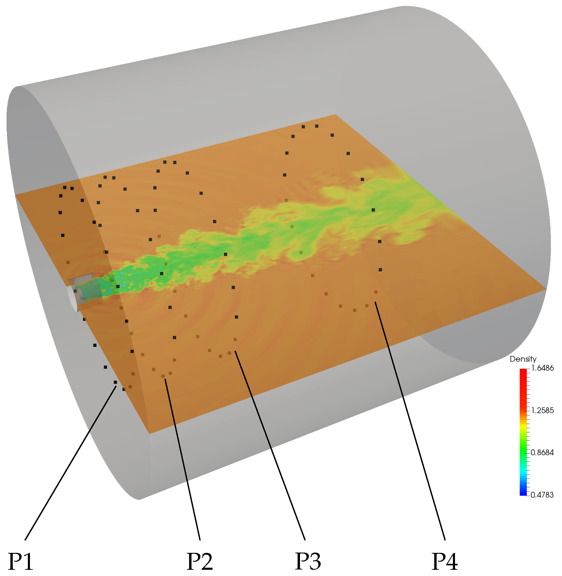
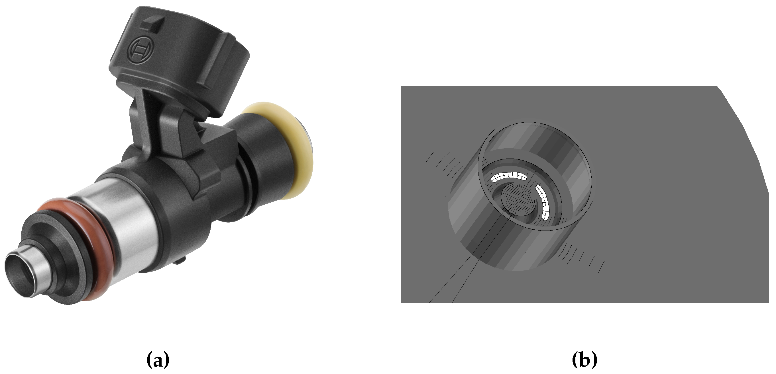
5.1. Simulation Case

We have evaluated our compression algorithm and adaptive compression framework based on a use case: simulation of the flow behavior of gas injection. For our simulation we use the original geometry of a natural gas injector (NGI) as shown in Figure 4a. This injector is used in a number of compressed natural gas powered vehicles. For this paper, we focus on the external flow behind the injector. Within this flow, shocks and turbulent shear layers are present, which emit pressure waves. From these pressure signals we can derive sound pressure levels (SPLs) directly from the simulation. The injector has four kidney shaped exits. We apply a direct aeroacoustic simulation, which allows us to calculate the sound pressure level directly from the simulation data. The compressed natural gas exits the four kidney shaped orifices at supersonic conditions and under expanded supersonic jets form. The normal velocity, pressure, density and Mach number are $w=505$ ms${}^{-1}$, $p=244$ kPa, $\rho =1.97$ kg m${}^{-3}$ and $Ma=1.21$. The simulations are performed on 163,691 DG-elements with an order of $N=4$.

Each element has ${(N+1)}^3=125$ degrees of freedom which leads to 20,461,375 degrees of freedom. For each DOF the conservative variables $\mathit{u}={(\rho ,\rho {\upsilon }_1,\rho {\upsilon }_2,\rho {\upsilon }_3,\rho e)}^T$ are stored. The surface mesh of the external injector is shown in Figure 4b. For a more detailed description of the geometry and the boundaries we refer to Kraus et al. [33]. The simulation is in excellent agreement with experiential data from [34]. The data compression used here are performed on all conservative variables, which are double precision floating point.

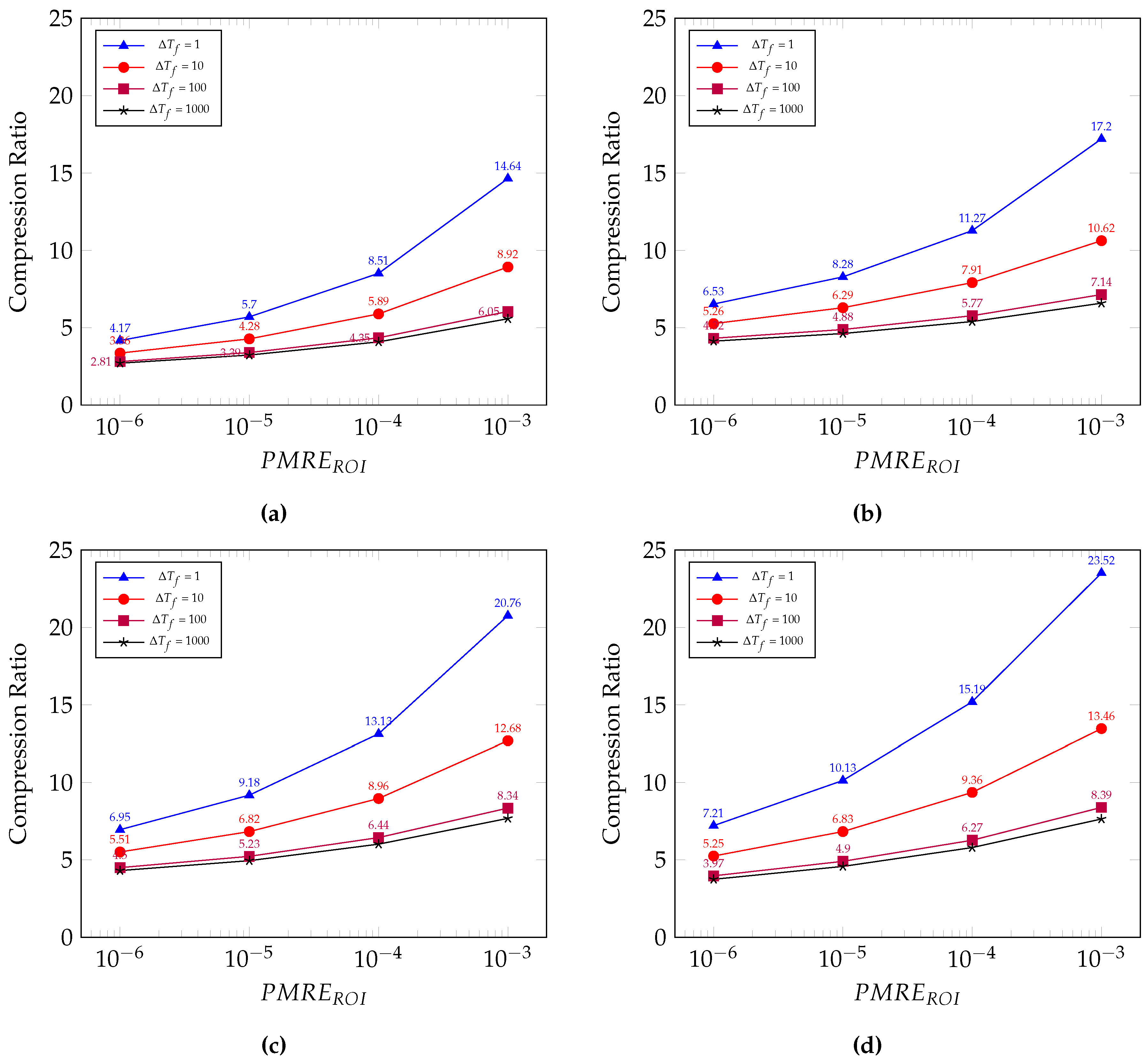
5.2. Compression Ratio

Figure 5 shows the compression ratio comparison at different permissible maximum relative errors and for four different $\Delta T_f$ and different framework configurations. $\Delta T_f$ indicates the lapsed simulation time between subsequent simulation frames that are stored (measured in number of time steps). In our simulation, a time step corresponds to ≈5 ns, and the compression ratio is defined as the ratio of the uncompressed data size to the compressed data size.

Figure 5a shows the compression ratio comparison without considering ROIs. It can be observed that the smaller $\Delta T_f$ the higher the compression ratio. The reason is that by having a smaller $\Delta T_f$ the prediction module predicts better, which leads to smaller residuals. For instance, when $\Delta T_f=1$, the compression ratio range from $4.17$ to $14.64$. For $\Delta T_f=1000$, the compression ratio decreases significantly, ranging between 2.8 and 6. From the result it can also be observed that after increasing $\Delta T_f$ above a certain value, the compression ratios remain almost constant. For instance the compression ratios for $\Delta T_f=100$ and $\Delta T_f=1000$ are almost identical. This indicates that, for large gaps between two time steps the predictor module no longer brings any advantages, and the remaining compression ratio is mainly due to the quantization module and the lossless compression algorithm. This is expected and in such cases, the algorithms that exploit spatial correlation or higher degrees predictors are recommended.

Figure 5b shows the compression ratio comparison considering ROIs. In this evaluation, the ROI is defined based on the temperature range. The temperature of all the nodes in one DG-element is measured, and if one of them has a temperature over 300 K, that DG-element is considered within the ROI. The $PMR{E}_{non-ROI}$ is equal to ${10}^{-2}$, and the $PMR{E}_{ROI}$ varies from ${10}^{-3}$ to ${10}^{-6}$. In this evaluation almost 50% of the DG-elements are in the region of interest, and the comparison with the previous configuration shows an average improvement of 30%. Figure 5c shows the compression ratio comparison considering ROIs and activating the reordering module. It can be seen that by reordering the nodes of each DG-elements and grouping the prediction residual of each parameter together, leads to an average improvement of 10% compared to the previous configuration. Figure 5d shows the compression ratio comparison considering ROIs with the condition being a temperature of less than 300 K. In this case, the ROI data values have much smaller variance and are more predictable than the previous ROI, which has more turbulences, leading to higher compression ratios.

5.3. Compression Performance

Figure 6 shows the relation between compression throughputs and compression ratio by applying different lossless compression algorithms. For this evaluation the throughput is defined as the original size divided by the required time to compress the data. Three different lossless compression algorithms namely, Bzip2 [28], Zlib [29] and FSE [30] are used in the compression framework. The Zlib library uses the LZ77 algorithm followed by a Huffman coding, whereas the Bzip2 algorithm first applies a Burrows–Wheeler transform on the data, followed by a run length encoding and also a Huffman coding. Finite state entropy (FSE) is a fast entropy encoder that has the same level of performance as Arithmetic coder, but only requires additions, masks, and shifts. Therefore, it is much faster than the other lossless compression algorithms. Our results show that it is almost 10 times faster than Bzip2 and six-times faster than Zlib. This benchmark is highly dependent on the data sets and requires online monitoring of the performance and compression ratio which is done by the proposed adaptive compression framework.

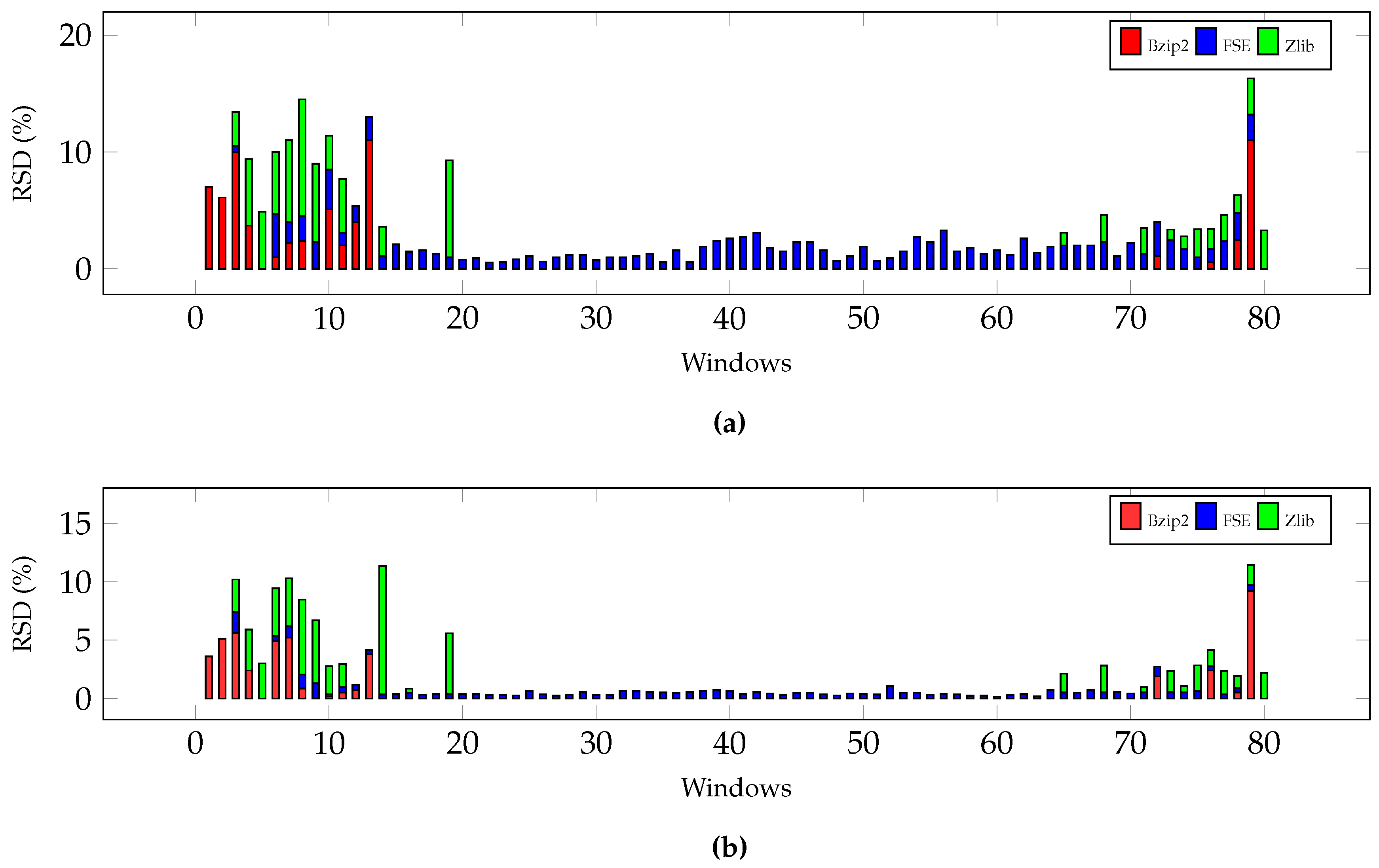
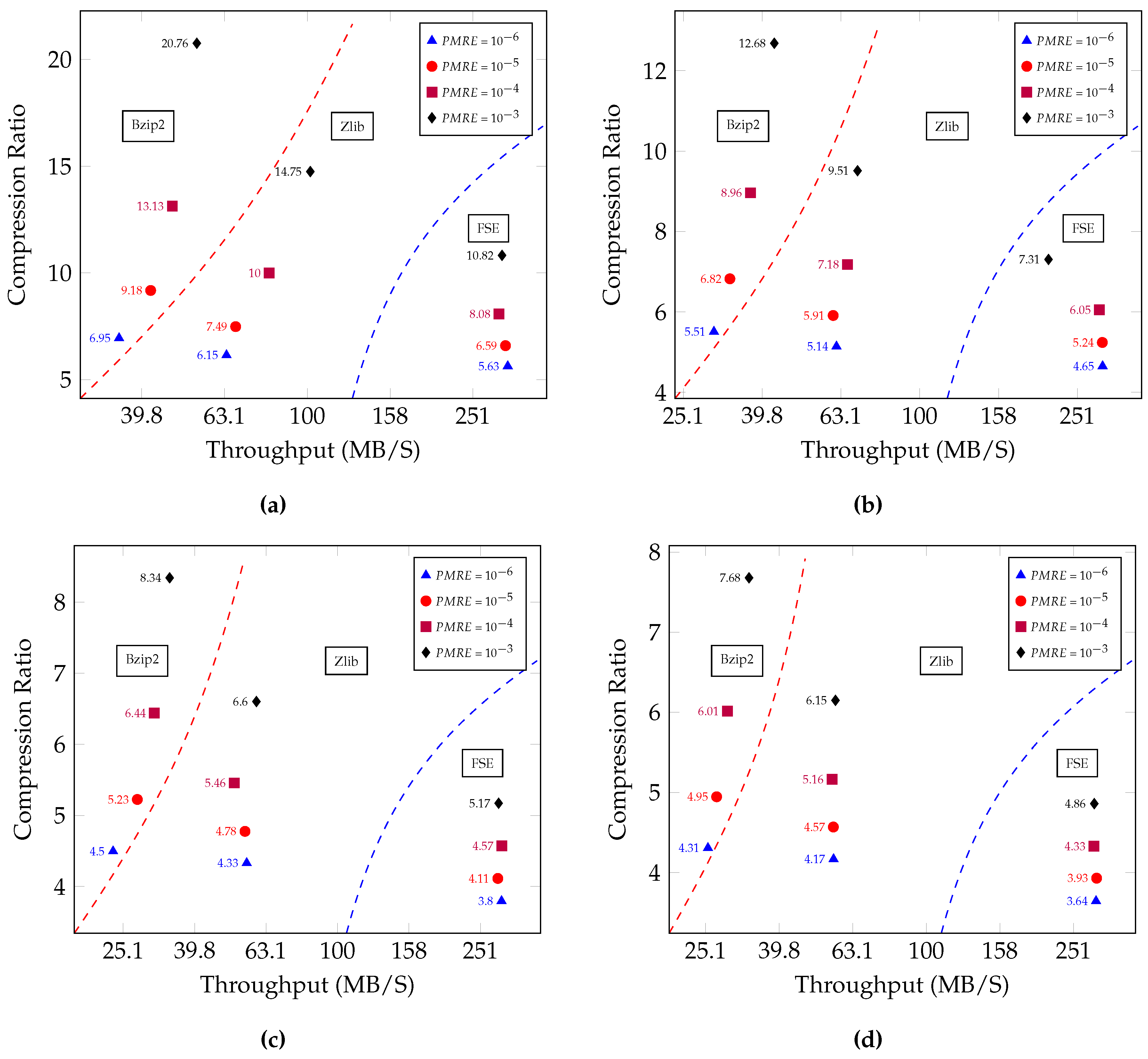
5.4. Compression Algorithm Comparison

In order to evaluate the compression efficiency of this work, we have made comparisons with five lossy compression algorithms, which are applicable to floating point simulation data. The following tests were conducted on a Core i7-3520M CPU @ 2.9GHz. For these comparisons, the throughput is defined as the amount of original size divided by the required time to compress the data.

Table 1. The comparison of the compression ratio for three different PMRE.

PMRE	${10}^{-3}$	${10}^{-4}$	${10}^{-5}$
Proposed Algorithm $\Delta T_f$ = 1000, 100, 10, 1	6.4, 7, 10.7, 17.8	4.6, 4.8, 6.7, 10.3	3.4, 3.6, 4.7, 6.4
Lorenzo Predictor-1D	8.1	5.4	3.9
Lorenzo Predictor-2D	9	5.9	4.2
Lorenzo Predictor-3D	9.48	6.28	4.5
FPZIP	6.7	5.4	4
ZFP *	7.9	4.1	2.6
ISABELA	3.9	2.9	2.4

* mean relative error is considered instead of PMRE.

and

Table 2. The throughput comparison for three different PMRE. Throughput unit is MB/s.

PMRE	${10}^{-3}$	${10}^{-4}$	${10}^{-5}$
Proposed Algorithm $\Delta T_f$ = 1000, 100, 10, 1	30.9, 33.1, 37.2, 47.1	24.2, 25.4, 32.7, 36.2	22.3, 22.9, 25.3, 31.8
Lorenzo Predictor-1D	32.3	28.8	23.1
Lorenzo Predictor-2D	36.2	30.4	23.6
Lorenzo Predictor-3D	36.9	30.3	25.6
FPZIP	89.1	73.1	63.5
ZFP *	63.97	54.21	40.1
ISABELA	3.7	4.4	5.1

* mean relative error is considered instead of PMRE.

list the compression ratio and the throughput comparison between the proposed algorithm and seven other lossy compression algorithms. In order to have a fair comparison, no ROI was considered for these comparisons. This means that $PMR{E}_{ROI}$ is equal to $PMR{E}_{non-ROI}$. All algorithms exploit the correlations of nearby values either spatial or temporal, and all of them are performed on structured $5\times 5\times 5$ DG-element.

The first three comparisons involved changing the temporal predictor with three types of Lorenzo predictor while keeping all the other aspects of the algorithm unchanged for fair comparison. Three categories of Lorenzo predictors are shown in Figure 7. The value of the corner “p” should be predicted by adding the value of the green corners and subtracting to the value of the red corners. In case of 1D Lorenzo only a neighboring value is considered as the predicted value, in this case $p(x,y,z,t)=a(x-1,y,z,t)$ and if $x=0$ then $p(0,y,z,t)=0$. The variable $a(x,y,z,t)$ indicates the value of the point $(x,y,z)$ at the time t. The proposed method is also in one dimension but in time, i.e., $p(x,z,y,t)=a(x,z,y,t-1)$. The 2D Lorenzo is applied in xy plane, where $p(x,y,z,t)=a(x-1,y,z,t)+a(x,y-1,z,t)-a(x-1,y-1,z,t)$. Similarly, the 3D Lorenzo predictor uses full 3D spatial prediction. For the boundary samples to be predicted, one layer of zero is padded in each dimension as proposed by [20]. Due to the lossy compression, all predicted values are updated by reconstructed values since these values are only ones available to the decompressor [20]. In this evaluation, Bzip2 [28] is used as a lossless compression algorithm for all compression algorithm. By comparing the compression ratios it can be observed that the three dimensional Lorenzo predictor has the highest compression ratio among the other algorithms. The proposed algorithm can only outperforms it when $\Delta T_f$ is less than 100.

FPZIP is the next algorithm which is considered in our benchmarking list [20,23]. FPZIP also applies the three dimensional Lorenzo predictor, however the compression is less than three dimensional Lorenzo that is discussed earlier. In the previous case we used the adaptive quantization method that is explained in Section 3.3 followed by Bzip2 which is a complex and slow lossless compression algorithm, while FPZIP performs different residual computation. However, due to the fast and optimized entropy encoder, FPZIP has the highest throughput among the other compression algorithms which are listed in Table 2.

ZFP is another compression algorithm that is considered for comparison [24]. ZFP handles three dimensional structure, therefore no dimension conversion is required. However, ZFP cannot bound the maximum relative error, therefore mean relative error instead of PMRE were ensured experimentally by varying the precision. The results shows that ZFP is among the fastest compression algorithms and has the second rank after FPZIP, and it is almost two times faster than the proposed compression algorithm in combination with Bzip2.

The last algorithm which is used for comparison is ISABELA, in which the relative error can be bounded [18]. In the first step each three dimensional DG-element is converted to a single dimension. Therefore, the ISABELA window size has 125 double precision floating point data. These data are sorted before performing the compression by B-spline interpolation. We have considered 10 points for B-spline curve fitting algorithm. In order to gain more compression ratio, Bzip2 is performed in the last step. The results shows that neither compression ratio nor throughput are comparable with other compression techniques. The main reason is that the ISABELA is originally designed for the data set which are random and noisy, which is not the case for the considered simulation data. Furthermore, sorting algorithm and B-splines curve fitting significantly degrade the throughout.

The combined information of Table 1 and Table 2 gives a holistic view on the interplay between compression ratio, throughput and quality (PMRE) and equips simulation experts with a greater degree of freedom. In case of the proposed algorithm, the compression ratio and the throughput is dependent on $\Delta T_f$ as evident from both Table 1 and Table 2. It can be observed that the proposed algorithm performs better than the other algorithms when the $\Delta T_f<100$. As $\Delta T_f$ increases the performance of the proposed algorithm drops in comparison to most other compression algorithms discussed in this work, however, even at $\Delta T_f=1000$ the proposed algorithm is still able to outperform state of the art compressor like ZFP for $PMRE\le {10}^{-4}$.

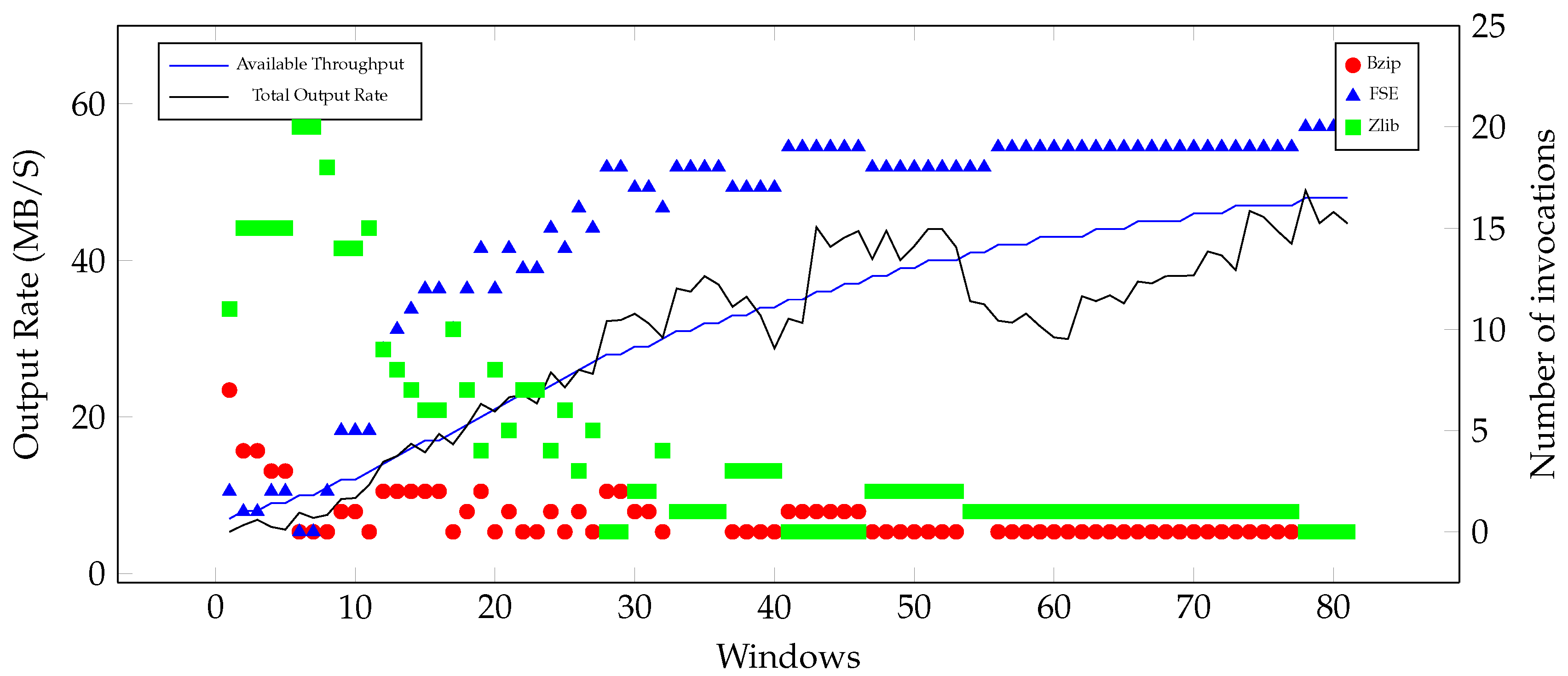
5.5. Adaptive Compression

The ability of the framework to optimize the dynamic selection of the lossless compression algorithm during run time is shown in Figure 8. In this example three lossless compression algorithms are considered. $WindowSize$ is equal to 20, which represents the number of subsequent frames in each windows, and $DS=$ 50,000 bytes. A fraction of the frames in each window is then compressed with Zlib, a fraction of them is compressed with Bzip2 and the rest with FSE encoder. In this evaluation the optimization algorithm was performed only once at the very beginning. The available throughput increases up to 50 MB/s. It can be seen that by invoking different lossless compression algorithms the total output rate follows the available throughput. If the total output rate is greater than the available throughput, the compressed data will be buffered.

In order to derive Equations (15) and (16) we assumed that each lossless compression algorithm has almost identical output rate and compression ratio in one window. To prove these assumption we calculated the relative standard deviation (RSD) of the compression ratio and output rate of each lossless compression algorithm in each window. Let $C_{ij}$ be the compression ratio of the i-th algorithm at the j-th frame of a window, and $s_i$ the frame position that the i-th algorithm start compressing the data . Then the relative standard deviation of the compression ratio of the i-th compression algorithm is given by:

$$RS{D}_{C,i}=100\%\times \frac{\sqrt{\frac{1}{x_i}{\displaystyle \sum _{j=s_i}^{x_i}}{(C_{ij}-\overline{C_i})}^2}}{\overline{C_i}},$$

(21)

where $\overline{C_i}$ denotes the average compression ratio of all the frames in a window that are compressed with i-th compression algorithm. The same equation also holds for output rate, the relative standard deviation of the output rate of the i-th compression algorithm is given by:

$$RS{D}_{R,i}=100\%\times \frac{\sqrt{\frac{1}{x_i}{\displaystyle \sum _{j=s_i}^{x_i}}{(R_{ij}-\overline{R_i})}^2}}{\overline{R_i}},$$

(22)

where $\overline{R_i}$ denotes the average output rate of all the frames in a window that are compressed with i-th compression algorithm. $RS{D}_{C,i}$ and $RS{D}_{T,i}$ are calculated for 80 windows, where each window contains 20 frames. The results are shown in Figure 9a for compression ratio and Figure 9b for output rate respectively. It can be observed that the maximum deviation from the average value in the worst case is around 15% for the compression ratios and almost 10% for the output rates. This is an indication that we can assume that each lossless compression algorithm provides almost identical compression ratio and output rate in one window.

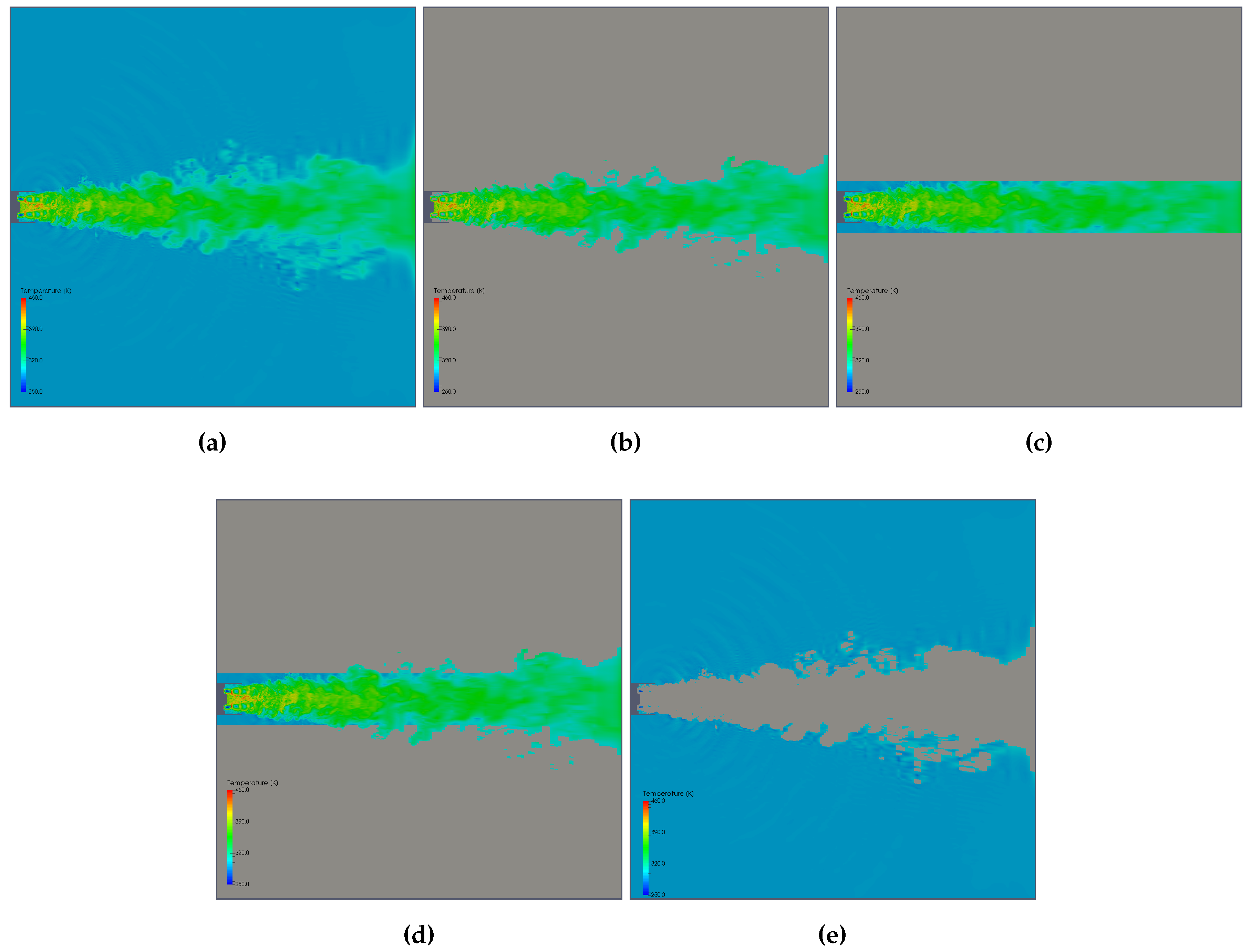
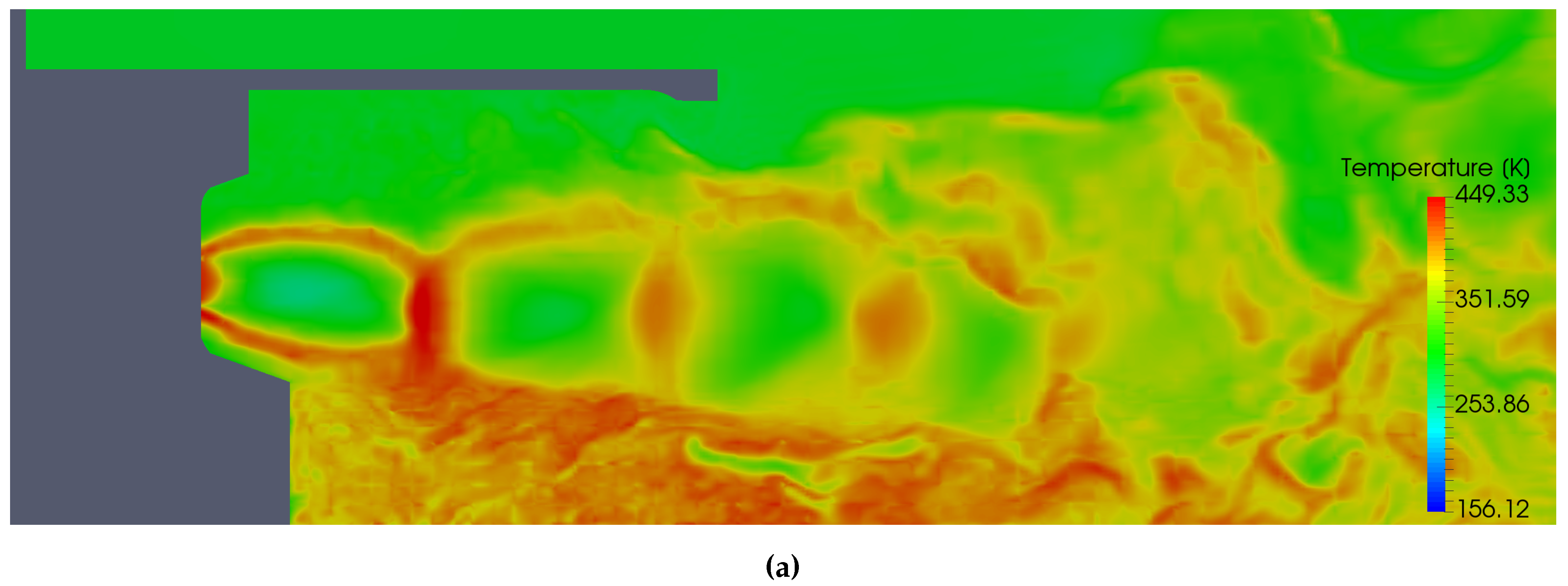
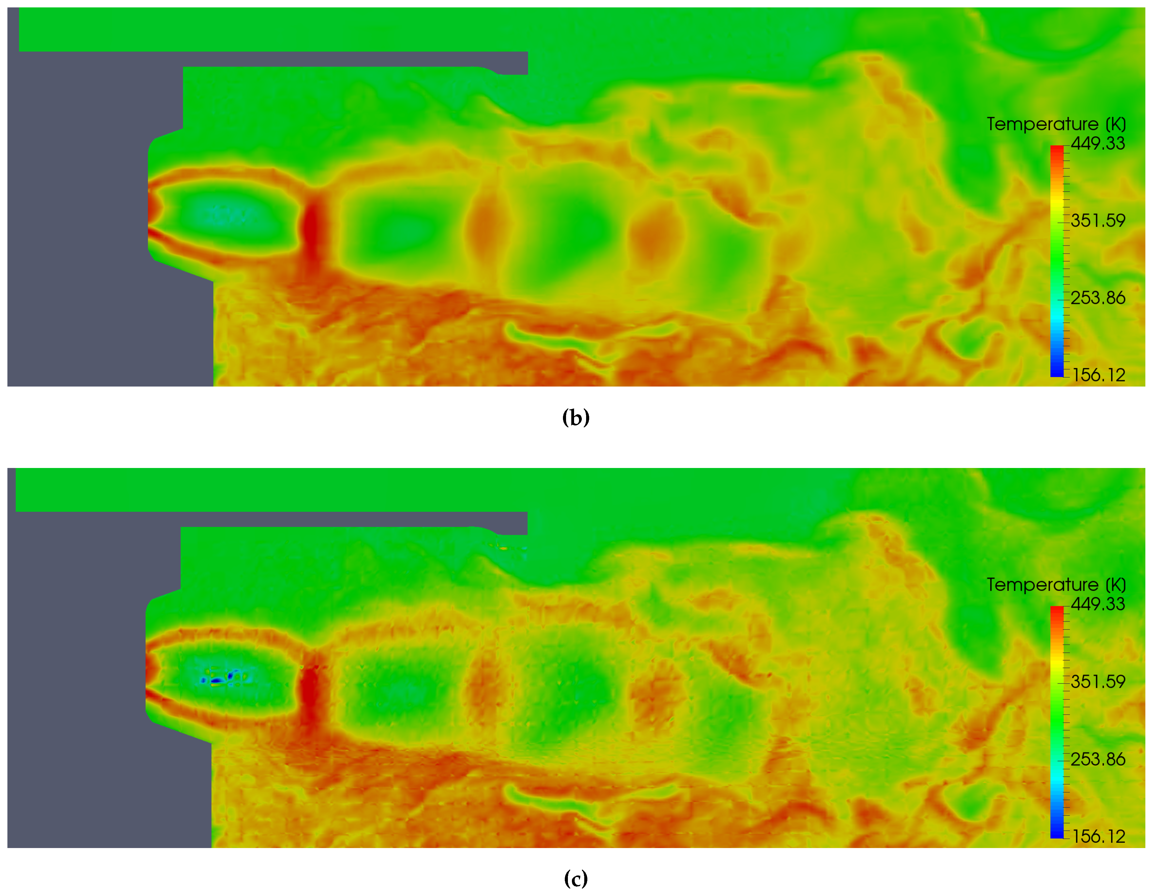
5.6. Temperature Analysis

In this section, the effect of lossy compression on the temperature (T) is investigated. The Temperature unit is Kelvin and is computed as:

$$T=\frac{p}{\rho R_s},$$

(23)

where the $R_s$ is the specific gas constant, $\rho$ is the density, and pressure (p) is given by:

$$p=(\kappa -1)(\rho e_{tot}-\frac{1}{2}\rho {\upsilon }^2),$$

(24)

where $\kappa$ is the heat capacity ratio and the velocity is computed as:

$$\upsilon =\sqrt{{\upsilon }_1^2+{\upsilon }_2^2+{\upsilon }_3^2}.$$

(25)

In order to assess the quality of the decompressed data, three quality measures are considered: maximum relative error (MRE), maximum absolute error ($\mid e{\mid }_{max}$) and root mean square error (RMSE); where,

$$MRE=max(\frac{\mid T_i-{\widehat{T}}_i\mid }{T_i}),$$

(26)

$$\mid e\mid {}_{max}=max(\mid T_i-{\widehat{T}}_i\mid ),$$

(27)

and:

$$RMSE=\sqrt{\frac{1}{i-n}{\displaystyle \sum _{i=1}^n}{(\mid T_i-{\widehat{T}}_i\mid )}^2},$$

(28)

where $T_i$ refers to the temperature of each point with the scale of Kelvin and, ${\widehat{T}}_i$ is the corresponding reconstructed value.

Table 3. Comparison of the decompressed data quality for ROI and non-ROI, as well as corresponding compression ratios.

Cons. Var.		Temperature						Compression Ratio
PMRE		MRE		$\mid \mathit{e}\mid {}_{\mathit{max}}$		RMSE
ROI	non-ROI	ROI	non-ROI	ROI	non-ROI	ROI	non-ROI	$\Delta T_f=1$
${10}^{-2}$	${10}^{-1}$	0.0397	0.34	14.60	149.4	2.7	2.07	38.77
${10}^{-3}$	${10}^{-2}$	0.0043	0.032	1.43	14.57	0.28	1.42	20.76
${10}^{-4}$	${10}^{-3}$	0.00042	0.0030	0.13	1.4	0.0277	0.22	11.88
${10}^{-5}$	${10}^{-4}$	0.00004	0.0003	0.014	0.14	0.0027	0.023	7.54

lists the MRE, $\mid e{\mid }_{max}$, RMSE and compression ratio (C) for ROI and non-ROI with respect to the various $PMR{E}_{ROI}$ and $PMR{E}_{non-ROI}$ of the conservative variables. In this evaluation, a DG-element is considered in the ROI if it has a temperature above 300 K. The $PMR{E}_{non-ROI}$ is taken to be one order of magnitude larger than $PMR{E}_{ROI}$. It can be seen that in the first evaluation where $PMR{E}_{ROI}={10}^{-2}$, the achieved compression ratio is very high. However, the quality of the decompressed data is low. In this case the maximum absolute error of almost 10 degrees for the ROI should be expected. It can be observed that the accuracy of the temperature improves by the same factor as the conservative PMRE improvement. A decent trade off between compression ratio and decompressed data quality can be seen in the third evaluation, where $PMR{E}_{ROI}={10}^{-4}$ and the maximum absolute error is almost 0.1 K. In this case a compression ratio of around 11 is achievable. Another fact is that the relative error of the temperature value is increased by four times compared to the relative error of the conservative values. The reason is that the relative error will be increased by arithmetic operations that are required to calculate the temperature value. For a more detailed description of error propagation we refer to [35].

Figure 10 shows the influence of the lossy data compression for the visualization of the temperature distribution. Figure 10b illustrates that by setting $PMR{E}_{ROI}$ to ${10}^{-3}$ and $PMR{E}_{non-ROI}$ to ${10}^{-2}$, a compression ratio of up to 20.76 can be achieved and the decompressed data are visually identical to the original data. However, by introducing more loss, as it it can be observed in Figure 10c, the data can be compressed almost two times more than the previous case, but an absolute error of up to 14.6 K in region of interest can occur.

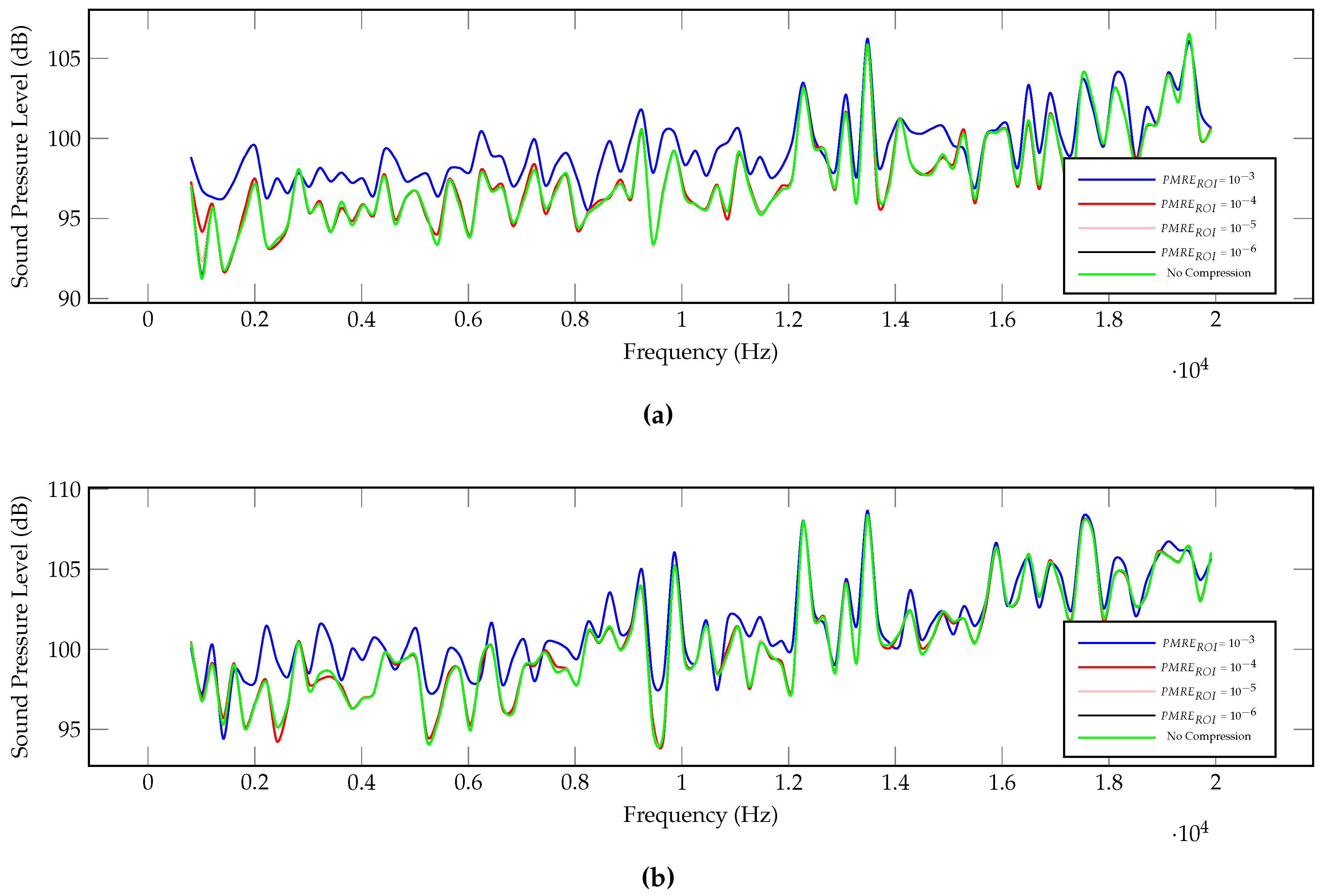
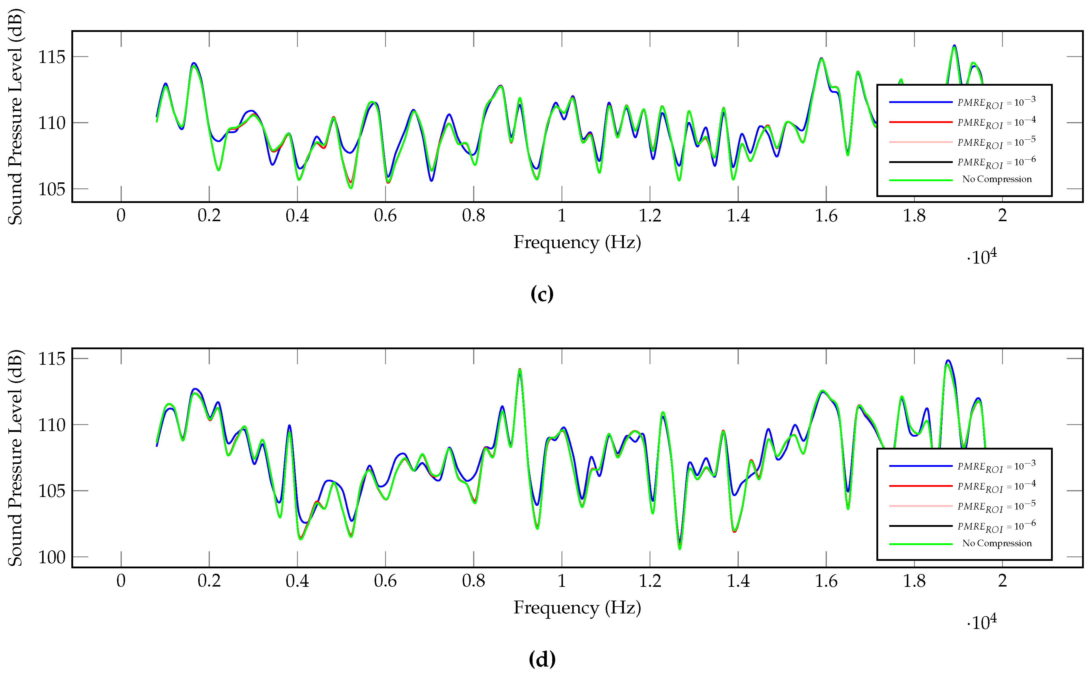
5.7. Sound Pressure Level Analysis

The sound pressure level (SPL) is used for measuring the magnitude of sound. SPL is the ratio between the actual sound pressure and a fixed reference pressure. The reference pressure is usually taken to be 20 micro pascals. For analyzing the effect of lossy compression on SPLs we have followed the simulation set–up proposed by [33,34], which has been shown to reproduce experimental data very accurately.

As is depicted in Figure 11, four observation areas, P1-P4, are considered for calculating the SPL, each consisting of 20 points. The pressure signals for each point are recorded at every time step and are averaged over 20 evenly distributed points around the center line axis. Afterwards, a transformation from the pressure signals to a SPL spectra is performed.

For this evaluation the regions which have the temperature less than 300 K are considered as ROIs, and compression ratio of up to 23.5 is achieved. Figure 5d shows the obtained compression ratios under different configurations.

Figure 12 shows the reconstructed and the original SPL spectra for P1-P4. As can be seen for $PMRE\le {10}^{-4}$, the reconstructed SPL are almost identical to the original SPL. In case of $PMRE={10}^{-3}$, the reconstructed SPL follows the trend of the original SPL but has a maximum absolute deviation of 5 db. However, if the peak value of the SPL spectrum is the value of interest, which is the case for some applications [36], the reconstructed SPL shows nearly the same peak values as the original SPL. This is an indication that even highly compressed data can be used effectively for SPL analysis. It is worth to mention that averaging over 20 points reduces the inaccuracy which may be caused by the quantization.

6. Conclusions

In this work, an adaptive prediction-based lossy compression scheme for compressing CFD simulation data is introduced to overcome storage requirements and I/O bandwidth limitation. In the proposed method, the inaccuracy caused by the lossy compression is adjustable and depends on the post processing requirements and ROI. In this work, the ROIs are indicated by a specified temperature range and are detected at run time. Additionally, by introducing an adaptive compression framework, the compression modules can adapt to the available network throughput. The proposed compression algorithm and adaptive compression framework are evaluated by the investigation of the flow behavior of gas injection. For our simulation, we use the original geometry of a natural gas injector, which is used in a number of compressed natural gas-powered vehicles. The compression ratios depend on the requested accuracy and the time interval between the stored simulation frames. The experimental results have shown that the compression ratio can easily vary from 2.8 to 23.5, and an average of 90% reduction in the data size is achievable. As a primary contribution of this work, we have shown that with reasonable choices for the permissible maximum relative error due to compression, the accuracy of post processing analysis such as sound pressure level and temperature measurements remain reliable. The lossless compression algorithms that are used in this paper are general purpose; more advanced and suitable lossless compression algorithms are considered as a future work.

References

1. Strohmaier, E.; Dongarra, J.; Simon, H.; Meuer, M. Top500 List—June 2016. Available online: https://www.top500.org/list/2016/06/ (accessed on 5 June 2016).
2. Hindenlang, F.; Gassner, G.J.; Altmann, C.; Beck, A.; Staudenmaier, M.; Munz, C.D. Explicit discontinuous Galerkin methods for unsteady problems. Comput. Fluids 2012, 61, 86–93. [Google Scholar] [CrossRef]
3. Atak, M.; Beck, A.; Bolemann, T.; Flad, D.; Frank, H.; Munz, C.D. High Fidelity Scale-Resolving Computational Fluid Dynamics Using the High Order Discontinuous Galerkin Spectral Element Method. In High Performance Computing in Science and Engineering, Transactions of the High Performance Computing Center, Stuttgart (HLRS) 2015; Nagel, E.W., Kröner, H.D., Resch, M.M., Eds.; Springer: Cham, Switzerland, 2016; pp. 511–530. [Google Scholar]
4. Cetin, M.O.; Pogorelov, A.; Lintermann, A.; Cheng, H.J.; Meinke, M.; Schröder, W. Large-Scale Simulations of a Non-Generic Helicopter Engine Nozzle and a Ducted Axial Fan. In High Performance Computing in Science and Engineering, Transactions of the High Performance Computing Center, Stuttgart (HLRS) 2015; Nagel, E.W., Kröner, H.D., Resch, M.M., Eds.; Springer: Cham, Switzerland, 2016; pp. 389–405. [Google Scholar]
5. Burtscher, M.; Mukka, H.; Yang, A.; Hesaaraki, F. Real-Time Synthesis of Compression Algorithms for Scientific Data. In Proceedings of the International Conference for High Performance Computing, Networking, Storage and Analysis, SC ’16, Salt Lake City, UT, USA, 13–18 November 2016; IEEE Press: Piscataway, NJ, USA, 2016; pp. 23:1–23:12. [Google Scholar]
6. Treib, M.; Bürger, K.; Wu, J.; Westermann, R. Analyzing the Effect of Lossy Compression on Particle Traces in Turbulent Vector Fields. In Proceedings of the 6th International Conference on Information Visualization Theory and Applications, Berlin, Germany, 11–14 March 2015; pp. 279–288. [Google Scholar]
7. Laney, D.; Langer, S.; Weber, C.; Lindstrom, P.; Wegener, A. Assessing the Effects of Data Compression in Simulations Using Physically Motivated Metrics. In Proceedings of the International Conference on High Performance Computing, Networking, Storage and Analysis, SC ’13, Denver, CO, USA, 17–22 November 2013; ACM: New York, NY, USA, 2013; pp. 76:1–76:12. [Google Scholar]
8. Baker, A.H.; Hammerling, D.M.; Mickelson, S.A.; Xu, H.; Stolpe, M.B.; Naveau, P.; Sanderson, B.; Ebert-Uphoff, I.; Samarasinghe, S.; de Simone, F.; et al. Evaluating lossy data compression on climate simulation data within a large ensemble. Geosci. Model Dev. 2016, 9, 4381–4403. [Google Scholar] [CrossRef]
9. Toro, E.F. Riemann Solvers and Numerical Methods for Fluid Dynamics—A Practical Introduction, 3rd ed.; Springer: Berlin/Heidelberg, Germany, 2009. [Google Scholar]
10. Schmalzl, J. Using standard image compression algorithms to store data from computational fluid dynamics. Comput. Geosci. 2003, 29, 1021–1031. [Google Scholar] [CrossRef]
11. Kang, H.; Lee, D.; Lee, D. A study on CFD data compression using hybrid supercompact wavelets. KSME Int. J. 2003, 17, 1784–1792. [Google Scholar] [CrossRef]
12. Sakai, R.; Sasaki, D.; Nakahashi, K. Parallel implementation of large-scale CFD data compression toward aeroacoustic analysis. Comput. Fluids 2013, 80, 116–127. [Google Scholar] [CrossRef]
13. Sakai, R.; Sasaki, D.; Obayashi, S.; Nakahashi, K. Wavelet-based data compression for flow simulation on block-structured Cartesian mesh. Int. J. Numer. Methods Fluids 2013, 73, 462–476. [Google Scholar] [CrossRef]
14. Sakai, R.; Sasaki, D.; Nakahashi, K. Data Compression of Large-Scale Flow Computation Using Discrete Wavelet Transform. In Proceedings of the 48th AIAA Aerospace Sciences Meeting Including the New Horizons Forum and Aerospace Exposition, Orlando, FL, USA, 4–7 January 2010; Volume 1325. [Google Scholar]
15. Sakai, R.; Onda, H.; Sasaki, D.; Nakahashi, K. Data Compression of Large-Scale Flow Computation for Aerodynamic/Aeroacoustic Analysis. In Proceedings of the 49th AIAA Aerospace Sciences Meeting Including the New Horizons Forum and Aerospace Exposition, Orlando, FL, USA, 4–7 January 2011. [Google Scholar]
16. Ballester-Ripoll, R.; Pajarola, R. Lossy volume compression using Tucker truncation and thresholding. Vis. Comput. 2016, 32, 1433–1446. [Google Scholar] [CrossRef]
17. Austin, W.; Ballard, G.; Kolda, T.G. Parallel Tensor Compression for Large-Scale Scientific Data. In Proceedings of the 2016 IEEE International Parallel and Distributed Processing Symposium (IPDPS), Chicago, IL, USA, 23–27 May 2016; pp. 912–922. [Google Scholar]
18. Lakshminarasimhan, S.; Shah, N.; Ethier, S.; Ku, S.H.; Chang, C.S.; Klasky, S.; Latham, R.; Ross, R.B.; Samatova, N.F. ISABELA for effective in situ compression of scientific data. Concurr. Comput. Pract. Exp. 2013, 25, 524–540. [Google Scholar] [CrossRef]
19. Iverson, J.; Kamath, C.; Karypis, G. Fast and Effective Lossy Compression Algorithms for Scientific Datasets. In Lecture Notes in Computer Science, Processings of the Euro-Par 2012: Parallel Processing Workshops, Rhodes Island, Greece, 27–31 August 2012; Kaklamanis, C., Papatheodorou, T., Spirakis, P.G., Eds.; Springer: Berlin/Heidelberg, Germany, 2012; pp. 843–856. [Google Scholar]
20. Lindstrom, P.; Isenburg, M. Fast and Efficient Compression of Floating-Point Data. IEEE Trans. Vis. Comput. Graph. 2006, 12, 1245–1250. [Google Scholar] [CrossRef] [PubMed]
21. Chen, Z.; Son, S.W.; Hendrix, W.; Agrawal, A.; Liao, W.K.; Choudhary, A. NUMARCK: Machine Learning Algorithm for Resiliency and Checkpointing. In Proceedings of the International Conference for High Performance Computing, Networking, Storage and Analysis, SC ’14, New Orleans, LA, USA, 16–21 November 2014; IEEE Press: Piscataway, NJ, USA, 2014; pp. 733–744. [Google Scholar]
22. Lakshminarasimhan, S.; Shah, N.; Ethier, S.; Klasky, S.; Latham, R.; Ross, R.; Samatova, N.F. Compressing the Incompressible with ISABELA: In-Situ Reduction of Spatio-Temporal Data. In Lecture Notes in Computer Science, Processings of the 17th International European Conference on Parallel and Distributed Computing Euro-Par 2011, Bordeaux, France, 29 August–2 September 2011; Jeannot, E., Namyst, R., Roman, J., Eds.; Springer: Berlin/Heidelberg, Germany, 2011; pp. 366–379. [Google Scholar]
23. Lindstrom, P. FPZIP Version 1.1.0. Available online: https://computation.llnl.gov/casc/fpzip (accessed on 10 March 2017).
24. Lindstrom, P. Fixed-Rate Compressed Floating-Point Arrays. IEEE Trans. Vis. Comput. Graph. 2014, 20, 2674–2683. [Google Scholar] [CrossRef] [PubMed]
25. Ibarria, L.; Lindstrom, P.; Rossignac, J.; Szymczak, A. Out-of-core compression and decompression of large n-dimensional scalar fields. Comput. Graph. Forum 2003. [Google Scholar] [CrossRef]
26. Sayood, K. Introduction to Data Compression, 2nd ed.; Morgan Kaufmann Publishers: San Francisco, CA, USA, 2000. [Google Scholar]
27. Fout, N.; Ma, K.L. An Adaptive Prediction-Based Approach to Lossless Compression of Floating-Point Volume Data. IEEE Trans. Vis. Comput. Graph. 2012, 18, 2295–2304. [Google Scholar] [CrossRef] [PubMed]
28. Seward, J. bzip2. Available online: http://www.bzip.org/ (accessed on 20 October 2016).
29. Gailly, J.; Adler, M. zlib. Available online: http://www.zlib.net/ (accessed on 20 October 2016).
30. Collet, Y. New Generation Entropy Codecs: Finite State Entropy. Available online: https://github.com/Cyan4973/FiniteStateEntropy (accessed on 20 October 2016).
31. Schrijver, A. Theory of Linear and Integer Programming; John Wiley & Sons, Inc.: New York, NY, USA, 1986. [Google Scholar]
32. Boblest, S.; Hempert, F.; Hoffmann, M.; Offenhäuser, P.; Sonntag, M.; Sadlo, F.; Glass, C.W.; Munz, C.D.; Ertl, T.; Iben, U. Toward a Discontinuous Galerkin Fluid Dynamics Framework for Industrial Applications. In High Performance Computing in Science and Engineering’ 15; Heidelberg, S.B., Ed.; Springer: Heidelberg, Geramny, 2015; pp. 531–545. [Google Scholar]
33. Kraus, T.; Hindenlang, F.; Harlacher, D.; Munz, C.D.; Roller, S. Direct Noise Simulation of Near Field Noise during a Gas Injection Process with a Discontinuous Galerkin Approach. In Proceedings of the 33rd AIAA Aeroacoustics Conference, Colorado Springs, CO, USA, 4–6 June 2012. [Google Scholar]
34. Hempert, F.; Hoffmann, M.; Iben, U.; Munz, C.D. On the simulation of industrial gas dynamic applications with the discontinuous Galerkin spectral element method. J. Therm. Sci. 2016, 25, 250–257. [Google Scholar] [CrossRef]
35. Ku, H.H. Notes on the use of propagation of error formulas. J. Res. Natl. Bur. Stand. C Eng. Instrum. 1966, 70, 263–273. [Google Scholar] [CrossRef]
36. Robinson, M.; Hopkins, C. Effects of signal processing on the measurement of maximum sound pressure levels. Appl. Acoust. 2014, 77, 11–19. [Google Scholar] [CrossRef]
Figure 1. A block diagram of the proposed compression algorithm.
Computation 05 00024 g001
Figure 2. A snapshot of the temperature of the external flow flow behind a gas injector: (a) without ROI; (b) ROI is defined based on the temperature range, ROI condition: T > 300 K; (c) ROI is defined based on the position of DG-elements; (d) ROI is a combination of (b) and (c); (e) ROI is defined based on the temperature range, ROI condition: T < 300 K.
Computation 05 00024 g002
Figure 3. A block diagram of the individual components of the compression framework, and their interaction with each other.
Computation 05 00024 g003
Figure 4. The real world use case behind the CFD simulations considered here: (a) natural gas injector with the injector outlet at the bottom left and (b) the surface mesh of the computational model for the injector outlet [32].
Computation 05 00024 g004
Figure 5. Each sub-figure shows the compression ratio comparison for different P M R E R O I and for various Δ T f . The configuration of the: (a) ROI and Reordering modules are not enabled; (b) only ROI module is enabled, ROI condition: T > 300 K , P M R E n o n R O I = 10 2 ; (c) both ROI module and Reordering modules are enabled, ROI condition: T > 300 K , P M R E n o n R O I = 10 2 ; (d) both ROI module and Reordering modules are enabled, ROI condition: T < 300 K , P M R E n o n R O I = 10 2 .
Computation 05 00024 g005
Figure 6. Relation between compression throughputs and compression ratios for different configurations while considering three different lossless compression algorithms. ROI condition: T > 300 K , P M R E n o n R O I = 10 2 . (a) Δ T f = 1 ; (b) Δ T f = 10 ; (c) Δ T f = 100 ; (d) Δ T f = 1000 .
Computation 05 00024 g006
Figure 7. Three different types of Lorenzo predictor [25] that are applied for comparison.
Computation 05 00024 g007
Figure 8. Dynamic adaptation of the compression algorithm to available throughput by varying the number of the lossless compression algorithm invocations for each window.
Computation 05 00024 g008
Figure 9. (a) The relative standard deviation of the compression ratio of each lossless compression algorithm in each window; (b) the relative standard deviation of the output rate of each lossless compression algorithm in each window.
Computation 05 00024 g009
Figure 10. Influence of the data compression on the visualization of the temperature distribution, ROI condition: T > 300 . (a) Original data; (b) decompressed data, P M R E R O I = 10 3 , P M R E n o n R O I = 10 2 , C = 20.76; (c) decompressed data, P M R E R O I = 10 2 , P M R E n o n R O I = 10 1 , C = 38.77.
Computation 05 00024 g010aComputation 05 00024 g010b
Figure 11. The kidney-shaped orifices and the simulation domain behind the injector with a cutting surface. The cutting surface shows a snapshot of the density. Four sets of observation points (P1 to P4) with different distances to the orifice are defined.
Computation 05 00024 g011
Figure 12. Shows sound pressure level spectrum with various P M R E R O I at four different areas: (a) P1; (b) P2; (c) P3; (d) P4.
Computation 05 00024 g012aComputation 05 00024 g012b