
Numerical Modelling of Double-Steel Plate Composite Shear Walls


School of Civil Engineering, Aristotle University, GR-541 24 Thessaloniki, Greece
*
Author to whom correspondence should be addressed.
Computation 2017, 5(1), 12; https://doi.org/10.3390/computation5010012
Submission received: 22 December 2016
/
Revised: 9 February 2017
/
Accepted: 13 February 2017
/
Published: 22 February 2017
(This article belongs to the Special Issue Selected Papers from the 7th International Conference from Scientific Computing to Computational Engineering (IC-SCCE 2016))
Abstract
:Double-steel plate concrete composite shear walls are being used for nuclear plants and high-rise buildings. They consist of thick concrete walls, exterior steel faceplates serving as reinforcement and shear connectors, which guarantee the composite action between the two different materials. Several researchers have used the Finite Element Method to investigate the behaviour of double-steel plate concrete walls. The majority of them model every element explicitly leading to a rather time-consuming solution, which cannot be easily used for design purposes. In the present paper, the main objective is the introduction of a three-dimensional finite element model, which can efficiently predict the overall performance of a double-steel plate concrete wall in terms of accuracy and time saving. At first, empirical formulations and design relations established in current design codes for shear connectors are evaluated. Then, a simplified finite element model is used to investigate the nonlinear response of composite walls. The developed model is validated using results from tests reported in the literature in terms of axial compression and monotonic, cyclic in-plane shear loading. Several finite element modelling issues related to potential convergence problems, loading strategies and computer efficiency are also discussed. The accuracy and simplicity of the proposed model make it suitable for further numerical studies on the shear connection behaviour at the steel-concrete interface.
1. Introduction
Composite construction is more and more frequently implemented in building structures and especially in shear walls, which are undoubtedly one of the most critical elements in a high-rise structural system. Double-steel plate concrete composite walls are composed of steel plates anchored to the infill concrete using welded stud shear connectors. Although steel plate and reinforced concrete shear walls are traditionally used as axial and seismic load-resisting systems, composite wall construction can offer a wide range of benefits. Double-steel plate concrete walls allow for modular construction leading to important cost and time saving. Steel faceplates can be fabricated offsite and then assembled and filled with concrete onsite. Steel faceplates serve both as concrete formwork and as primary reinforcement. In addition, this system has superior blast and impact resistance.
The two major fields on which this system can be widely used are multi-storey buildings and nuclear facilities. Design requirements differ for each case. Applications of double-steel plate concrete walls to the containment of internal structures (enclosures around a nuclear reactor to confine fission products that might be released to the atmosphere if an accident occurred) and shield building in nuclear facilities have begun in the United States and China, based on the work of Varma and his partners at Purdue University [1,2,3,4]. Additionally, based on the experimental and numerical work of Varma, Appendix 9, which refers to composite construction, has been added to the existing US standards (ANSI/AISC N690) [5,6]. In contrast, as refers to the design of building structures, a double-steel plate concrete wall should not only be designed to work over the elastic limit, but also to obtain a significant amount of ductility during the post-elastic stage. Consequently, it is evident that the focus of the accomplished research was the elastic response and further investigation is needed regarding nonlinear response and seismic behaviour of double-steel plate concrete walls.
1.1. Numerical Literature Overview
Vecchio and McQuade [7] adapted the Distributed Stress Field Model, a smeared rotating crack model for reinforced concrete based on the Modified Compression Field Theory, to the analysis of steel and concrete wall elements under axial and shear loads. The computational model was then incorporated into a two-dimensional nonlinear finite element analysis algorithm using the two-dimensional nonlinear finite element analysis program Vector2 [8]. A perfect bond was assumed between the steel faceplates and infill concrete. The critical buckling stress proposed by Usami et al. [9] has been adopted. The accuracy of the model was proved using experimental results reported in the literature [9,10,11]. In all cases, the analysis model was found to provide accurate calculations of shearing strength, but the stiffness at displacements lower than those associated with peak strength was significantly overestimated [7]. Additionally, deficiencies were found in terms of faceplate buckling and interfacial slip between steel and concrete.
Zhou et al. [12] developed a 2D finite element model to simulate the cyclic response of double-steel plate concrete walls. They used membrane elements with plane stress behaviour to model the infill concrete and the steel faceplates. The finite element model did not include the connectors and the steel faceplates were tied to the infill concrete. The Cyclic-Softened-Membrane-Model developed by Mansour et al. [13,14] has been validated using experimental data of a reinforced concrete (RC) shear wall [15] and then it was used to model the infill concrete in combination with a plasticity model for steel faceplates. The numerical model was not validated. The parameters considered in the investigation were wall thickness and faceplate slenderness ratio.
Ma et al. [16] conducted a numerical study on double-steel plate concrete walls under axial compressive and cyclic lateral loadings to investigate the effects of the axial force and steel faceplate thickness on the response of double-steel plate concrete walls. Concrete was modelled with smeared-crack solid elements, whereas steel faceplates were simulated with piece-wise-linear plastic shell elements with isotropic hardening. Hard interfacial contact was assumed to avoid penetration of the steel faceplates into the infill concrete. The skeleton curve obtained from the predicted hysteretic curve was divided into three stages, namely elastic, elastic-plastic (cracking of the concrete core and yielding of steel faceplates) and hardening (buckling of steel faceplates). Post-peak strength response has not been considered. The proposed model successfully predicted the shear strength of the walls but underestimated the displacement at peak force.
Rafiei et al. [17] used ABAQUS [18] to simulate the behaviour of a composite shear wall system consisting of profiled steel sheeting and a concrete core under in-plane monotonic loading. They conducted a parametric study to investigate the effects of the configuration of the intermediate fasteners along the height and width of the wall, the steel yield and the concrete compressive strength. They developed a detailed and a simplified numerical model and proved that the simplified numerical model was more efficient in terms of computation time and accuracy.
Ali et al. [19] developed an ABAQUS model [18] to simulate the response of four I-shaped (walls with flanges) double-steel plate concrete walls with varying steel plate thickness in the web and flanges. In order to model the infill concrete and the steel faceplates, concrete damage plasticity (CDP) and bilinear kinematic hardening models were used respectively. The concrete core and the steel plates were modelled using solid elements. The nodes of the flange wall were tied to the nodes of the web. The numerical results matched the experimental behaviour with reasonable accuracy in the pre-peak stage of response.
Varma et al. [3] developed a simple mechanistic representation of the in-plane shear behaviour of double-steel plate concrete walls and a design equation for calculating their in-plane stiffness and strength. The model was verified using experimental results reported in the literature [11] and a large-scale in-plane shear test conducted by Varma et al. [3]. Nevertheless, the numerical model had important limitations. It did not include concrete cracking and post-cracking behaviour in tension. In addition, it did not directly account for concrete inelasticity in compression and the analysis was terminated if the minimum principal concrete compressive stress exceeded 70% of the compressive strength. Finally, a fully bonded interaction between steel and concrete was assumed. To overcome these limitations, Varma et al. [4] developed a layered composite shell finite element model using ABAQUS [18]. However, the numerical peak shear strength predicted by both models was less than the experimental peak shear strength of the composite walls. Analytical and numerical models have been used to generate in-plane force and out-of-plane moment interaction curves. However, in order to use this approach, the wall cross-section should be detailed with adequate shear connectors and transverse tie bars so as to prevent brittle failure modes like local buckling of the faceplates before yielding, out-of-plane shear failure and interfacial shear failure.
Kurt et al. [20] developed a finite element model using explicit analysis [21] to study the monotonic in-plane shear behaviour of double-steel plate concrete walls. Afterwards, they conducted a parametric study to study the influence of wall thickness and aspect ratio on the response of composite walls. Epackachi et al. [22] also used LS-DYNA [21] to develop a numerical model and simulate the nonlinear cyclic response of composite shear walls. They used 2-node beam elements to model each shear connector and coupled one of the nodes to concrete elements. The assumption of a perfect bond between the faceplates and infill concrete resulted in a conservative prediction of the post-peak resistance of the composite walls. However, it may also affect the pre-peak response for different faceplate slenderness ratios, defined as the spacing of the connectors to the thickness of the faceplates.
Vazouras and Avdelas [23] studied the behaviour of double-steel plate concrete walls under monotonic and cyclic horizontal loading using the ANSYS Mechanical finite element package [24]. The objective of the research was to evaluate the influence of fundamental parameters of its response, such as aspect ratio and thickness of steel plates and to study the behavioural curve, the capacity under both compressive and bending conditions, the ductility and the failure process. Shear connectors have not been modelled. Therefore, the numerical model assumed a perfect bond between the faceplates and infill concrete using tie constraints. Since the focus of the investigation was not the behaviour of shear connectors, the model provided reasonable results for composite walls designed using a dense spacing of shear connectors.
In conclusion, the majority of the aforementioned numerical studies focused on the behaviour of composite walls before achieving the peak load. Furthermore, the majority of them assumed the steel nodes tied to the concrete nodes and did not address the effects of steel faceplate buckling and spacing of connectors on the in-plane response.
1.2. Objectives and Scope of Work
This paper proposes a new three-dimensional finite element model, developed using the software ANSYS 15.0 [24], incorporating a detailed description of the modelling process, material properties, element types, boundary conditions and application of loads. The most important aspect of this model is that although it uses low order elements, it can result in an accurate prediction of the structural elastic and post-elastic response of a double-steel plate concrete wall.
Two cases have been identified in terms of loading types imposed on composite walls, namely axial compression loading and monotonic, cyclic in-plane shear loading. The first loading case is critical for the relative motion between faceplates and infill concrete, whereas the second one is significant to investigate the seismic behaviour of double-steel plate concrete walls. Different modelling assumptions are adopted in each case in order to maintain reasonable accuracy in predicting the response of double-steel plate concrete walls. This approach resulted in a numerical model that can effectively describe the major loading conditions on composite walls in a reasonable time and with significant accuracy.
The numerical model generally accounted for the nonlinear monotonic and cyclic responses of the steel faceplates and the infill concrete, friction between the two materials and presence of connectors (studs and possible steel side plates). The inclusion of shear connectors, contact elements and friction in the steel-concrete interface was necessary to accurately simulate the behaviour of double-steel plate concrete walls. Furthermore, the numerical model addressed the effect of modelling the foundation of a composite wall, since its flexibility could considerably influence global response.
The accuracy of the numerical model was verified using data from tests of six experimental programs reported in the literature [9,11,22,25,26,27]. The cases listed above were selected because they not only describe comprehensively geometric, material and structural response details, but also four of them examined compression loading, whereas the rest accounted for in-plane shear loading. Considering the analysis results, the developed finite element model is proposed as being suitable for design purposes and further parametric studies.
Finally, it should be noted that the focus of this research is the description of a structural system for building construction which consists of prefabricated steel plates serving as permanent concrete formwork and filled with concrete. Other possible configurations such as two thin steel faceplates connected through the concrete infill (which are impractical for building construction due to the need for thermal insulation etc.) are out of the scope of this research. Furthermore, the effect of concrete reinforcement may be beneficial, but it provokes other construction problems, which can be easily solved with the use of shear connectors. Additionally, steel plates serve as reinforcement. Positioning the faceplates at the extreme fibre of the cross-section not only maximises their influence on flexural resistance but also provides tension reinforcement in all directions. This cannot be achieved in reinforced concrete walls due to clear cover requirements. Thus, for the same section depth, the moment capacity and flexural rigidity are inherently larger and simultaneously the resulting deflections are smaller for a composite wall than in a reinforced concrete one of the same thickness. Alternatively, it is evident that the required capacities for building construction are easily achieved with this wall type without adopting large section thickness. Even in the case of double-steel plate concrete walls used in nuclear facilities [1,2,3,4,20,27], where a larger wall thickness is needed due to the need for radiation shielding and where transverse tie bars instead of reinforcing bars are being used to join the steel plates, their role is to enhance the structural integrity of the cross-section and not the capacity. As a result, providing further reinforcement in a concrete core to enhance the capacity of a double-steel plate concrete wall is out of the scope of this research.
2. Numerical Model Formulation
The numerical study was undertaken using the ANSYS 15 finite element analysis program [24]. The following sections briefly describe the modelling properties and assumptions. The finite element model accounted for the nonlinear behaviour of materials, the nonlinear interfacial shear force-slip behaviour of shear studs, the local buckling of the steel plates associated with geometrical nonlinearity and was capable of nonlinear static and dynamic analysis so as to capture the effects of concrete cracking and crushing.
2.1. Analysis Method
Overall, two major analysis finite element analysis methods can be used: implicit or explicit. The majority of the researchers used explicit analysis to model the behaviour of composite walls, due to the difficulty in modelling the nonlinear behaviour of concrete. Bruhl et al. [1], Sener et al. [2] and Varma et al. [3,4] used explicit analyses for the analysis of double-steel plate concrete walls used in nuclear facilities. Epackachi et al. [22] also used explicit analyses for the analysis of composite walls used in multi-storey buildings. In contrast, Vazouras and Avdelas [23] used implicit analyses to analyse the behaviour of composite walls, assuming tied connection between steel and concrete nodes.
In the case of an implicit analysis, the calculation of current quantities in one time-step is based on the quantities calculated during the previous time step. This procedure is called Euler Time Integration Scheme. In this scheme even if large time steps are chosen, the solution remains stable. In contrast, an explicit solution is unstable as it does not utilise the Euler Time Integration Scheme. The use of very small time steps is needed to overpass this problem. Another difference is that the implicit algorithm requires the calculation of the inverse of the stiffness matrix, whereas the explicit algorithm requires the inversion of the mass matrix, which can be diagonal if lower order elements are used. As a result, in a static loading case, it is preferable to use implicit analysis, in which big time steps can be used and the solution can be obtained in a few iterations. For these reasons, implicit analysis has been used in this research for the investigation of the performance of double-steel plate concrete walls.
Additionally, it should be noted that in an implicit analysis nonlinearities can be modelled even better than in explicit analysis because every parameter of the material behaviour and every property of the contact model can be controlled. As a result, the nonlinear behaviour of concrete has been represented accordingly. Furthermore, convergence in an implicit analysis is rather difficult (this is one of the reasons why many researchers choose explicit analysis), but when it is achieved the accuracy of the results is better. In general, this analysis method was considered ideal to study the general behaviour of a composite wall. On the other hand, explicit analysis can be used to focus on the behaviour of shear connectors. The results of this research will be presented in the future.
2.2. Element Types and Material Properties
2.2.1. Concrete Infill
Two concrete types were used in this research depending on the configuration of the cross-section: fully confined and partially confined. In the case of the composite wall, concrete has been considered as properly confined when steel side plates were welded to the faceplates to form a closed-formed rectangular steel section infilled with concrete as shown in Figure 1. Overall, the configuration of a composite wall depends on the existence or absence of boundary elements or the type of the building’s structural system. Consequently, although the existence of steel side plates may be beneficial to the performance of double-steel plate concrete, placing concrete in a triaxial stress state and providing structural integrity, their application may not be always feasible. As a result, concrete behaviour has been categorised into two groups namely confined (Figure 1) and partially confined (Figure 2). Different modelling strategies have been used for each case.
This approach came up during the validation procedure due to the different behaviour of concrete in the composite wall configurations exhibited in Figure 1 and Figure 2. This modelling approach has been validated using experimental results reported in the literature. To be more specific, wall specimens tested by Epackachi et al. [22], Ozaki et al. [11], Choi et al. [26] and Zhang [27] did not include side plates resulting in a partially confined concrete model, whereas specimens tested by Akiyama et al. [25] and Usami et al. [9] included side plates resulting in a fully confined concrete model. Additionally, it has been assumed that the confinement provided by the steel plates exceeds by far the confinement provided by the shear connectors and as a result, the latter has been neglected. This assumption has been proved during the validation procedure.
In general, modelling concrete behaviour was of great concern not only due to its different behaviour in tension and compression but also due to convergence difficulties in an implicit analysis procedure caused when concrete is not properly confined.
An eight-node 3D solid element (SOLID65) was used to properly model concrete behaviour. This element has three degrees of freedom at each node (translations in the nodal x, y and z directions) [28]. It is capable of plastic deformation, creep, cracking in the three orthogonal directions and crushing. The William-Warnke criterion [29] has been used as failure criterion due to multiaxial stress state. When concrete fails, the software sets the stiffness of the failed element to zero and proceeds to the next sub-step. This would eventually result in a non-convergence state meaning that the concrete has completely failed. Several trials have been made and it has been concluded that crushing of concrete in the first configuration provided accurate results, while it may lead to premature failure in the second configuration. Barbosa et al. [30] also reported premature indications of failure due to crushing, when the Solid65 crushing capability was turned on. They reported that the failure occurred due to concrete crushing, before reaching the experimental ultimate load. In this research, the same behaviour was observed for unconfined concrete.
As refers to confined concrete, the presence, at an integration point, of a crack has been represented through modification of the stress-strain relations. This has been done by the introduction of a weakness plane in a direction normal to the crack face [24]. Further, a shear transfer coefficient was introduced representing a reduction factor of shear strength that accounts for sliding (shear) across the crack face induced by subsequent loading. If the crack closes, then all compressive stresses normal to the crack plane are transmitted across the crack and only a shear transfer coefficient for a closed crack is introduced. If the material at an integration point fails in uniaxial, biaxial, or triaxial compression, then it is assumed that the material crushes at that point, with crushing defined as the case in which the structural integrity of the material deteriorates completely. Finally, the failure surface of the concrete has been defined by five strength input parameters. The shear transfer coefficients for an open and closed crack were 0.3 and 0.7, respectively. The stress relaxation coefficient was equal to the default value of 0.6. The characteristic yield stress in compression was determined based on either experimental data for the validation studies or on nominal material properties [31]. The ultimate tensile stress was determined based on Eurocode 2 (EC2) provisions [31].
Considering partially confined concrete, the crushing capability of element Solid65 has been turned off. Two alternative methods have been developed to define the concrete crushing failure using strains developed in concrete. The first method uses the maximum strain as an indication of failure. In general, the maximum strain is not a reliable measure for assessing the concrete crushing mode of failure since, although the capacity of the section is large enough to carry loads till crushing, strains propagate completely in the wall section. This causes certain points to experience high strains under the concentrated pressures, even when the wall is still in its elastic state limit. To eliminate this effect, the top endplates of each specimen need to be modelled in order to transfer the load to the composite section progressively, instead of omitting their existence and apply the pressure directly to the concrete elements. According to the second method, the concrete crushing is considered when the first contour line of a strain equal or larger than 0.0035 (value proposed by EC2 [31] and achieving the best correlation with experimental results) is formed all through the concrete width. Although both methods ended up to similar results regarding failure due to the crushing of the concrete infill, the first method has been adopted in order to explore the effects of modelling endplates on the general structural behaviour.
In all specimens, concrete reached its ultimate strength after 28 days. However, curves derived from compression tests were not available for these cases. As a result, each stress-strain curve was calculated separately for the ultimate compressive strength of every specimen. The nonlinear behaviour of concrete depicted in Figure 3 by an equivalent uniaxial stress-strain curve developed according to EC2 [31] has been adopted. This figure indicates the behaviour of concrete in tension and compression. As regards concrete in compression, the first part of the curve and until the proportional limit stress, was initially assumed to be in the elastic range. The proportional limit stress value was taken as equal to , where is the ultimate compressive cylinder strength of concrete. The strain associated with was equal to 0.0022. The Poisson ratio of the concrete was taken as equal to 0.2.
The second part of the curve is a nonlinear parabolic curve starting from and reaching to the concrete compressive strength . This part of the curve can be determined from Equation (1) given by EC2 [31], where is the stress at any strain , is the characteristic cylinder compressive strength of concrete, is the ratio of the strain at stress to the strain . At the peak compressive stress is equal to 0.0022 and is a parameter equal to
The third part of the stress-strain curve is a descending part from to a value of lower than or equal to , where is a reduction factor referred from the study of Ellobody et al. [32]. This factor varies from 1 to 0.5 corresponding to concrete cube strength from 30 to 100 MPa. In this study, was taken as equal to a constant value of 0.85. The ultimate strain of concrete at failure was equal to . According to EC2 [31], is equal to 0.0035 (). Ellobody et al. [32] considered equal to 11 in a confined concrete model. In the present study, an ultimate strain of 0.0035 () has been considered. As regards specimens with side plates, a higher value of has been assumed since concrete was under a triaxial state of stresses and its performance was enhanced.
2.2.2. Steel Plates
Due to the fact that steel plate thickness is rather small compared to its other dimensions, they have been considered as thin-walled elements [24,33]. This was a decisive fact for the selection of the appropriate finite element. A four node structural shell element (SHELL181) was used to represent the steel faceplates and possible side plates. Side plates are used only in specimens fabricated by Akiyama et al. [25] and Usami et al. [9] and this is another reason why these specimens were selected for this validation study. SHELL181 is suitable for analysing thin to moderately thick shell structures. It has six degrees of freedom at each node: translations in the x, y, z directions and rotations about the x, y, z-axes [28]. Additionally, it is well-suited for linear, large rotation and large strain nonlinear applications. Although the default option for this element is reduced integration with hourglass control, full integration with incompatible modes has been used in this study so as to achieve the best simulation of the deformed shape of a double-steel plate concrete wall due to buckling.
The constitutive material law selected to represent monotonic steel behaviour used the von Mises yield criterion with kinematic hardening rule. The Poisson ratio of steel was taken as equal to 0.3. The stress-strain relationship is shown in Figure 4, where is the yield stress, is the ultimate tensile strength, is the strain at the yield stress , is the strain at the beginning of strain hardening branch, is the strain at the ultimate strength . The first part of the curve is linear elastic up to yielding and the second part between the elastic limit () and the beginning of strain hardening () is perfectly plastic. The last part of the curve represents the strain-hardening branch and it was calculated according to the constitutive law used by Gattesco [34], given in Equation (2), where is the strain hardening modulus of steel
Under load reversals, the load-bearing capacity of a steel member generally decreases as the number of load cycles increases [34]. A large literature for steel constitutive models [35,36,37,38,39] has been studied to end up with the adopted cyclic response of steel shown in Figure 5. To account for progressive hardening and softening effects [40], steel was assumed to have a multilinear kinematic hardening behaviour as described above. Additionally, some isotropic effects have also been considered so as to account for the Bauschinger effect. This effect, upon load reversal in the direction of plastic deformation, shows a reduction in the yield stress.
2.2.3. Steel Endplates
As it has been discussed before, modelling of endplates was necessary in order to transfer the axial compressive loading to the composite section and obtain smooth strain contour results. Two alternatives have been studied, regarding the selection of the appropriate element type. At first, endplates were modelled using the same element with steel faceplates (SHELL181). As a result, concrete elements located near the contact surface of the endplate and the concrete infill deformed locally. As this behaviour did not come up during the experiment, it was concluded that SHELL181 does not properly model endplate behaviour. This fact can be justified since endplates used in experiments are relatively thicker than side plates so as to safely impose the compressive loads and they cannot be properly modelled using a shell element. Finally, a solid element (SOLID185) in the form of a homogenous structural solid has been used for modelling the endplates.
SOLID185 is defined by eight nodes having three degrees of freedom at each node: translations in the nodal x, y, and z directions [28]. Further, the element has plasticity, hyperelasticity, stress stiffening, creep, large deflection, and large strain capabilities. The Von Mises yield criterion with isotropic hardening rule was also used for the modelling of steel endplates.
2.2.4. Shear Connectors
There are many alternatives considering modelling of shear connectors. In this research headed studs have been used to guarantee composite action between steel and concrete. The case of overlapping shear connectors has been considered and it has been concluded that in the case of overlapping headed shear studs there is an interaction resulting in an augmented pull-out resistance. The beneficial effect of this interaction was neglected in this research and will be investigated in a future study.
In order to make the most efficient choice in terms of analysis time and modelling behaviour, the slenderness of a typical composite double-steel plate shear wall should be considered. Slenderness is defined as the ratio of the overall thickness of the wall to the height of each shear connector after the welding procedure. This ratio is calculated for every case considered in this research. It was concluded that the slenderness ratio is high enough to assume that each shear connector is exclusively defined by axial internal forces. As a result, nonlinear springs (COMBIN39) were used to represent the headed studs.
The element COMBIN39 has no mass and it is defined by two (preferably coincident) node points and a generalised force-deflection curve [28]. The need for coincident nodes demands the use of a common meshing for steel and concrete. Moreover, it has a longitudinal or torsional capability. The adopted longitudinal option is a uniaxial tension-compression element with, at each node, up to three degrees of freedom (translations).
Many researchers have selected nonlinear springs to model the shear connection between steel and concrete in composite beams [41,42]. Queiroz et al. [43] proposed a three-dimensional model, in which each shear connector has been modelled using a nonlinear spring (COMBIN39) parallel to the direction of the relative movement between the composite slab and the steel beam. On the vertical to the relative movement direction, nodes have been coupled. However, this assumption is not valid for double-steel plate concrete walls, since if the nodes are coupled, pry-out failure of headed studs will not be included as a possible failure mode of the specimen and as a consequence, the entire model will assume a full shear connection between faceplates and the infill concrete. In general, shear connectors used in composite walls not only offer shear but also tensile resistance.
In this paper, a simplified modelling approach for the shear connection behaviour in composite walls is proposed. Further, in previous studies, each shear connector has been modelled using one spring. In this research, every shear connector has been modelled using two springs: one parallel and one normal to the direction of the relative movement between faceplates and the infill concrete so as to simulate their shear and tension capacity. The inclusion of these springs requires as input data a load-slip curve. Either empirical formulations or curves obtained directly from available push-out tests [40] can be utilised. In this study, as there were no push-out test results available, the majority of the empirical formulations available in the literature have been studied in order to end up to a load-slip curve that fits better to the experimental behaviour of each specimen. Finally, the following load ()-slip () model proposed by Ollgaard et al. [44] has been adopted, Equation (3), where is the ultimate load capacity of a steel shear stud and the units are kilo-pound (kip) for load and inch (in.) for slip
The ultimate shear capacity of a shear stud is an indispensable parameter in load-slip models. The failure mode of the steel-concrete interface is quite complicated. Failure may occur in the concrete or in the shear connector. Typical concrete failures are breakout, pry out or localised crushing. On the other hand, the stud shank may fail in shear or the weld may fracture as well. Sometimes the failure can be mixed, including two or more of the failure modes mentioned above. Therefore, researchers proposed relations to calculate the load bearing capacity considering both concrete and steel properties. In this study, the following EC4 [40] provisions have been adopted.
The design shear resistance of a headed stud automatically welded should be determined from the minimum value derived from Equations (4) and (5), where is the partial factor (the recommended value is 1.25 for design, but in this study it is taken equal to 1 for comparison purposes), and are the shank diameter and the overall nominal height of the stud respectively, is the specified ultimate tensile strength of the material of the stud (its value cannot be greater than 500 MPa), is the characteristic cylinder compressive strength of the concrete (its density should not be less than 1750 kg/m3) and is a parameter calculated from Figure 6
The procedure listed above results to a multilinear load-slip curve for the first spring, which was placed parallel to the relative motion of steel plates and infill concrete. The second spring is characterised by the tensile strength of each headed stud, which is known either from preliminary tensile tests or the specifications of the manufacturer. In this study, the tensile capacity of headed studs has been calculated based on relations existing in the literature [45,46] and finally a multilinear load()-slip() curve has been used to model the behaviour of the second spring. The representation of the proposed model for shear connectors and details about their connection with steel and concrete at the interface are shown in Figure 7.
2.2.5. Contact Elements
The specimens used in this study achieve the mechanical interlock and the shear bond between steel and concrete with the use of shear studs. Friction forces are also developed at the interface. Regarding boundary contact conditions, contact and non-contact regions are not a priori known. This contact problem is called a unilateral problem with friction. This highly nonlinear problem has to be modelled in order to simulate the actual behaviour of a double-steel plate composite shear wall.
ANSYS software program [24] uses the Coulomb friction model for the formulation of this kind of contact problems as shown in Equation (6), where is the coefficient of friction, is the equivalent Coulomb friction shear stress and is the contact pressure at the steel-concrete interface. As soon as the shear stress at the steel-concrete interface exceeds the term , relative slip between steel plates and concrete occurs
Three-dimensional nonlinear surface-surface “contact pair” elements (CONTA173 & TARGE170) [28] have been used to model the nonlinear behaviour of the interfacial surface between infill concrete and steel plates in order to achieve composite action. The concrete and steel surfaces were assumed to be deformable. Contact elements overlay the elements used for modelling steel plates and infill concrete. Each contact pair has been constructed by using area to area contact element types. During the analysis, contact is detected at the Gauss points. However, due to the fact that contact boundary conditions differ across the model, different contact surface properties should be considered.
Concrete Infill—Steel Plates
Elements generated for this contact were able to simulate the existence or absence of pressure when there is contact or separation between them respectively. Regarding the friction coefficient, Rabbat et al. [47] concluded that the average coefficient of static friction should be taken between 0.57 and 0.7. In the present work it was not deemed negligible; instead, trials have been done using three different friction coefficients: 0.3, 0.5 and 0.7. It has been concluded that in the case of in-plane lateral loading, interfacial friction can be neglected since the variation of the friction coefficient did not affect the load-displacement curve of the analysed specimens. As a result, the comparison between friction coefficients has been conducted for compression loading.
Concrete Infill—Endplates
For this contact interaction, the same contact elements have been used. However, this contact is considered as continuously bonded. During the experimental procedure, this behaviour is ensured by welding the endplates to the faceplates and the possible side plates and by welding strong shear connectors to transfer gradually the applied load to the concrete infill.
2.2.6. Foundation
Experimental results reported by Epackachi et al. [22] indicated that the initial stiffness of composite walls constructed with a baseplate connected to a RC foundation may be substantially affected by the flexibility of the connection with a potentially significant impact on the dynamic response of the supported structure. In order to address this issue two different numerical models, namely detailed and simplified, as shown in Figure 8, have been developed to identify the importance of modelling the foundation for the seismic performance of the composite walls. The detailed models explicitly accounted for every construction detail of the foundation. However, foundations may differ in practice based on soil properties. Therefore, simplified models were also developed, where the base of the wall was assumed fixed using rigid zones on the base nodes of steel faceplates and concrete respectively. Beam elements were used to represent transverse tie bars. Specifically, the main objective of the comparison between detailed and simplified numerical models was to investigate the efficiency of simplified models to predict the in-plane shear strength of double-steel plate concrete walls with the understanding that ignoring the flexibility of the foundation may lead to an overestimation of the stiffness.
2.3. Meshing
ANSYS software [24] includes two different methods for mesh generation, the solid modelling method and the direct generation method. The solid modelling method requires from the user to describe the size, shape and boundaries of the whole object and to induce controls on the element types and mesh sizes. Then the software generates the elements, meshes and nodes automatically. On the other hand, in the direct generation method all the geometries, elements, meshes and nodes are to be defined by the user. Although the latter method is more time consuming, it has been adopted for this study since, regarding the multi-material problem (double-steel plate composite shear walls) which has to be solved, it was more beneficial and powerful in terms of control over the model and geometries.
Moreover, meshing the relatively thin steel plates is a quite challenging procedure. ANSYS [24] requires the size of an element to be within standard ratios in order to derive its three-dimensional stress distributions. If the dimension size ratio of an element is equal or less than 1/20, the program will generate shape ratio warnings. As a result, this stage demands a great attention and control of the shape warnings, which is granted by using the direct generation method.
A mesh refinement analysis has been conducted in order to obtain the best results regarding the analysis time (number of elements) and the realistic simulation of a composite wall. Three different mesh densities A, B and C have been examined as shown in Figure 9. The calculated discrepancies were 5.3%, 1.4% and 7.2% for Mesh A, Mesh B and Mesh C, respectively. Although all three simulations predicted similar results, it was noted that excellent results were obtained when the medium coarse Mesh B has been used. This may be attributed to the fact that several damage processes result in concrete damage and headed stud steel anchors deformation. As a result, Mesh B has been adopted for the finite element analysis. Finally, it should be noted that the results of the mesh refinement analysis were in complete agreement with the basic concepts of the finite element method. In the finite element modelling, as the number of elements increases, the stiffness of the system decreases since it gains higher indeterminacy and extra degrees of freedom. In other words, a higher number of elements provide the system with the ability to deform in a less rigid shape. As a result, a classic finite element composite wall model should demonstrate higher deformation as the number of element increases and this was the key parameter for choosing the appropriate mesh.
2.4. Loading
Compression loading has been applied at the top side of the endplate with the form of pressure as it is shown in Figure 9, whereas in-plane monotonic and cyclic lateral loading has been applied by imposing displacements at the top concrete and steel nodes as shown in Figure 8. As a result, shear has been applied in the form of uniform displacements. Displacement values were not divided, every steel and concrete node at the top side of the specimen had the same displacement.
Two load steps have been defined to distinguish the elastic and the plastic stage for each specimen. The first load-step was defined to go from the zero stress state up to the approximate yielding point of the wall. The second point can be determined from the experimental results, but it is better to choose this point conservatively. This load-step was given through a small number of sub-steps, as the software did converge easily because of the linear behaviour of the wall during this stage. After running the model, the exact yield point was determined and in the case that the actual yielding point was smaller than the assumed one, a small part of the nonlinear behaviour was already derived with less accuracy than the one required for the nonlinear part. Therefore, the model has been adjusted and run again. The second load step was assumed to go from yielding to failure. It is crucial as it indicates the nonlinear behaviour and ductility of the composite wall. In this study, the applied load was chosen to be 110% of the expected ultimate load. In this way, the model would continue to deform after failure and exactly record the failure mode and its initiation. As a result, the failure mode of each specimen has been accurately defined.
2.5. Nonlinear Solution and Convergence Criteria
The analysis performed accounted for geometrical and contact nonlinearities, stress stiffening and large deflections. The adopted Newton-Raphson [48] solution method implied incremental loading and solved the model for unknown displacements. According to this method, the incremental loading has been applied to the system and then a nonlinear system of equations was solved to derive the incremental displacements. The tangential stiffness matrix was updated after each iteration. The convergence procedure was force-based and thus considered absolute.
More specifically, this method solved a series of successive linear approximations. The finite element discretisation procedure resulted in three main matrices of coefficients, unknowns (degree of freedom displacements-DOFs) and loads. The problem is generally considered as nonlinear when the coefficient matrix itself is a function of unknown DOFs. Equations (7–10) exhibit the Newton-Raphson adopted procedure, where is the coefficient matrix, is the vector of unknown DOF values, is the vector of applied loads, is the Jacobian matrix of coefficients (tangent matrix), is the vector of restoring loads corresponding to the element internal loads, is the incremental displacements in the current iteration, is the subscript representing the current iteration and is the residual load vector. Specifically, Equation (7) is the original form and Equation (8) is the modified form proposed by Bathe et al. [49]
The solution of the problem derives from the following numerical procedure:
- (a)
- The first load step is considered as the load target that the model has to converge on .
- (b)
- The first incremental load vector is applied . It is a vector of restoring loads that corresponds to the internal loads of elements.
- (c)
- DOF values are assumed from the restoring displacements , which derive from the result of the previously convergence attempt or they are equal to zero at the first substep.
- (d)
- The software computes the Jacobean of the coefficient matrix based on the assumed DOFs .
- (e)
- Having obtained the incremental loads , the incremental displacement can now be calculated using Equation (8).
- (f)
- The incremental displacements will be added to the assumed values of displacements and form the second iteration shown in Equation (9). This creates a new vector of restoring loads based on the assumed values of displacements.
This iterative process ends when both the incremental displacement and the residual load vector lie in the convergence criteria. Then, the new target will be set on the next substep. In this study, 200 iterations are considered in each sub-step to achieve convergence. For example, a single iteration is depicted graphically in Figure 10a. Figure 10b shows the next iteration of this example.
3. Validation Results
3.1. In-Plane Shear Loading
3.1.1. Validation with First Set of Specimens
The accuracy of the developed finite element models was first verified using the experimental results reported by Epackachi et al. [22] because they comprehensively describe foundation detailing making the comparison of detailed and simplified models feasible. They tested four double-steel plate concrete walls under displacement-controlled cyclic loading. The dimensions and material properties of the specimens are summarised in Table 1, where is the height of the wall, is the length of the wall, is the thickness of the wall, is the thickness of steel plates, is the spacing of the headed studs, is the spacing of tie bars, is the measured yield stress of steel plates and is the concrete compressive strength. In specimens with headed studs and tie bars, the slenderness ratio of the faceplates is equal to the minimum value of and . The design variables considered in the testing program included spacing of the connectors and a reinforcement ratio equal to for the tested specimens, which included only two steel faceplates. Two of the specimens had only headed studs, whereas the rest had also transverse tie bars, which have been modelled using beam elements.
The validation procedure has been conducted for all the specimens, but since the general trend is the same, for brevity, only the load-displacement curves obtained from the FEM analysis of two specimens are plotted with respect to the test results, in Figure 11 and Figure 12. These figures include comparisons of the lateral force-lateral displacement curves predicted by the simplified and detailed numerical models with the corresponding experimental curves for specimens SC1 and SC4, respectively. As shown, the detailed models accounted for the foundation flexibility and successfully predicted the experimentally measured stiffness of the test specimens. On the other hand, the simplified models overestimated the stiffness but predicted the shear capacity and failure mechanism of the specimens with acceptable accuracy as shown in Figure 13. However, the simulation of a foundation is not always feasible since it depends on the overall design of the composite wall and the soil properties. For this reason, the simplified models with a fixed base could be used to preliminarily estimate their lateral load capacity using finite element analysis and as soon as detailing information is provided; the detailed models can be used for the calculation of the composite wall stiffness.
3.1.2. Validation with Second Set of Specimens
Ozaki et al. [11] tested nine double-steel plate concrete panels under cyclic in-plane shear, but two of them had additional stiffeners such as partitioning webs. As a result, only seven test specimens have been used for the validation studies listed in Table 1. There were three groups of specimens S2, S3 and S4 with reinforcement ratios of 2.3%, 3.4% and 4.5%, respectively. Specimens S2-00-NN, S3-00-NN and S2-00-NN were subjected to pure in-plane shear with no axial compression. They are included in Table 1 for comparison with specimens S2-15-NN and S3-15-NN that were subjected to 353 kN of axial compression producing an average compressive stress of 1.47 MPa and specimens S2-30-NN and S3-30-NN that were subjected to 706 kN of axial compression producing an average compressive stress of 2.94 MPa.
The in-plane shear force and shear strain response results from the finite element analysis have been compared with the experimental results as shown in Figure 14, Figure 15, Figure 16 and Figure 17. As shown, there is an excellent agreement between experimental and numerical results. Therefore, it has been concluded that the simplified finite element model can predict the behaviour of all the composite walls with or without axial forces with reasonable accuracy.
3.2. Compression Loading
The finite element models were validated using the experimental results reported by Akiyama et al. [25], Usami et al. [9], Choi et al. [26] and Zhang [27]. The dimensions and material properties of the specimens are summarised in Table 1. The comparison of experimental and numerical results including yield and ultimate strength and critical displacements are summarised in Table 2 for the first seven specimens listed in Table 1. Additionally, experimental and numerical load-deflection curves are compared in Figure 18, Figure 19, Figure 20, Figure 21, Figure 22 and Figure 23 for the remaining specimens. More specifically, the comparison between the three different mesh densities is presented in Figure 18, Figure 19, Figure 20, Figure 21, Figure 22 and Figure 23 and the comparison between the three different friction coefficients is presented in Figure 24, Figure 25, Figure 26 and Figure 27.
The validation of the numerical model has been conducted using all the developed meshing configurations A, B and C as shown in Figure 18, Figure 19, Figure 20, Figure 21, Figure 22 and Figure 23. All three simulations predicted almost identical results. Noticeable differences have been observed in the ultimate loads and slips, which are within the margin of error expected for a numerical simulation. Nevertheless, it was noted that excellent results were obtained when the medium coarse Mesh B has been used. This may be attributed to the fact that several damage processes result in concrete damage and deformation of headed stud steel anchors. As a result, Mesh B has been adopted for the finite element analysis.
The comparison between the three different friction coefficients is presented in Figure 24, Figure 25, Figure 26 and Figure 27. It is evident that the differences in the elastic range are negligible. Considering the post-elastic stage of the specimens, it is evident that a friction coefficient equal to 0.3 resulted in less capacity and ductility than the experimental one. In contrast, the capacity and the corresponding displacement declined as the friction coefficient augmented. Finally, a constant friction coefficient of 0.5 was considered as ideal for the simulation of the steel-concrete interface.
The results from these comparisons clearly prove that the numerical model perfectly predicts the elastic response of each specimen. However, after yielding the numerical results show a slightly different behaviour in the nonlinear part. It is observable that after yielding, the experimental load-deflection behaviour is slightly stiffer than the numerical results. This behaviour is attributed to the simplified strain hardening behaviour of steel that was considered in the finite element modelling.
Furthermore, the numerical results of this research have been compared with analysis results reported by Vazouras and Avdelas [23] in order to identify the importance of modelling the slenderness of the wall with the use of shear connectors and the unilateral contact between the steel plates and concrete with the use of contact elements on the seismic performance of double-steel plate concrete walls. In general, the assumption of a perfect bond between the steel plates and the infill concrete did not significantly affect the pre-peak strength response of the composite walls in the range of steel plate slenderness studied in this research [23]. However, the numerical post-peak resistance was less than the experimental value when a perfect bond was assumed. This fact is mainly attributed to premature fracture of the faceplates caused by the assumption of a perfect bond.
4. Parametric Analysis
4.1. Design Procedure
The objective of the parametric analysis was to investigate the influence of important parameters on the seismic behaviour of composite walls. This section summarises the results of a parametric study on the monotonic and cyclic lateral response of sixteen composite walls used to investigate the effects of the aspect ratio , reinforcement ratio , the yield strength of the faceplates and the uniaxial compressive strength of concrete on the in-plane response of SC walls. The geometric reinforcement ratio is defined as the steel area to the concrete area .
The dimensions and material properties of specimens in the parametric analysis are described analytically in Table 3. Two aspect ratios 0.75 and 2.0 have been considered to study the behaviour of low and high aspect ratio walls by setting the length of the specimens equal to 2000 mm and varying the height . Steel plates of S235 ( 235 MPa) and S355 ( 355 MPa) were selected to represent low and high values of yield strength, respectively. The ultimate steel tensile strength was calculated based on EC3 provisions [50] as 360 MPa and 510 MPa. The elastic modulus of steel was taken as equal to 210,000 MPa. The uniaxial concrete compressive strength was considered equal to 30 MPa and 40 MPa to represent low and high strength concrete, respectively.
In order to generate the cyclic behaviour of the composite shear wall, loading was simulated by applying the displacement control scheme rather than direct loading. A displacement-controlled, reversed cyclic loading protocol was used according to the recommendations of ACI 374.1-05 [51]. This loading protocol is based on imposing displacements proportional to the yield displacement of each specimen. For this reason, a monotonic analysis was conducted first up to the failure of each specimen and then the specimens were subjected to a cyclic alternating lateral force. Two additional loading steps at displacements equal to 10% and 75% of the reference displacement were added to the proposed deformation history to capture the wall response before and after cracking of the infill concrete. Additionally, the loading procedure was extended for each specimen by two more load steps after the failure load. Figure 28 presents the loading protocol used to test the first specimen. The loading protocol consisted of nineteen load steps with two cycles in each step. In each loading cycle, a push was imposed first, followed by a pull, where “push” was defined as the loading in the positive direction and “pull” was defined as the loading in the negative direction.
Key analysis results, in terms of monotonic and cyclic loading, are summarised in Table 4 and Table 5, respectively. The total shear force of the wall at yield , the maximum shear force and the failure lateral load are included in the analysis results. Additionally, the yield displacement , the displacement at the ultimate shear force , the displacement at failure and the corresponding drift ratios are listed in Table 4 and Table 5. The criteria used for the definition of the ultimate state and failure mode of each specimen were based on the degradation of the in-plane shear capacity. Specifically, failure was defined at 80% of the peak load [52], since it provided an excellent indication of the excessive deformation, mainly out-of-plane, at the bottom of the wall and excessive concrete cracking (especially during cyclic loading) and crushing.
4.2. Analysis Results
The first parameter evaluated was the effect of the aspect ratio on composite walls. It has been concluded that as the aspect ratio increased, the lateral load capacity and stiffness of double-steel plate concrete walls declined. Additionally, analysis results listed in Table 4 and Table 5 indicate that as the aspect ratio increased, the displacement corresponding to the peak shear force and the ductility augmented. Furthermore, buckling of the steel plates in high aspect ratio walls was not detrimental to performance and had a minimal effect on the ultimate shear strength and overall performance of the specimens. Similar results were obtained for the other values of concrete strength investigated in this research.
Additionally, the effect of reinforcement ratio on the in-plane response of the double-steel plate concrete walls has been investigated. Although the reinforcement ratio had a negligible effect on the initial stiffness and ductility, it significantly affected the lateral strength, namely lower reinforcement ratios led to less lateral capacity. Furthermore, it can be seen that an increase in the aspect ratio substantially reduced the effect of other design variables on the response of SC walls. However, the displacement at the peak shear force was not substantially affected by the reinforcement ratio.
Furthermore, the effects of concrete compressive strength and steel yield strength on the in-plane response of the composite walls have been evaluated. As refers to the first parameter, the yield and ultimate strength augmented as the concrete strength increased. In fact, the aspect ratio played a critical role, since the influence of the concrete compressive strength on the peak lateral load increased as the aspect ratio decreased. Considering the second parameter, the shear load capacity soared with the increase of steel yield strength. It can be noticed that the increase of steel yield strength had a more pronounced impact on specimens with aspect ratios lower than 2.0.
Finally, the comparison of cyclic and monotonic analysis results presented in Table 4 and Table 5 indicated that the difference between the capacities predicted through monotonic and cyclic analysis was negligible. This fact is mainly attributed to the exceptional post-elastic behaviour of steel. Specifically, its high tensile strength and ductility prevented the abrupt deterioration of the composite wall capacity due to the brittle behaviour of the concrete material characterised by crushing at the toes of the wall. In general, it can be concluded that a monotonic analysis can provide a good estimation of the general behaviour of composite walls. However, this conclusion should be further investigated with extensive parametric analysis.
5. Conclusions
The objective of this study was to develop a reliable three-dimensional finite element model for the nonlinear analysis of double-steel composite shear walls, focusing on the shear connection behaviour. For this purpose, the commercial finite element software ANSYS 15.0 [24] was used. Validation studies have been undertaken using the results of four axial compression and two in-plane shear experimental programs. Measured global and local responses have been used to validate the proposed model. Additionally, the importance of including foundation flexibility in the numerical model has been addressed. Furthermore, it has been shown that the introduction of interface contact friction elements between the infill concrete and the steel plates leads to a significant changing of the results especially for the post-peak range of response.
As a result, the nonlinear behaviour of a double-steel plate concrete wall can be predicted using:
- A multilinear stress-strain curve for concrete, using user-specified material properties. In the absence of experimental data, the curve can be estimated from relations proposed by EC2 [31]. In the case of partially confined concrete, the best way for indicating the concrete crushing failure mode is by evaluating the concrete strain contour results. Considering fully confined infill concrete, the William-Warnke criterion [29] can be used as failure criterion due to multiaxial stress state.
- A multilinear stress-strain curve for steel based on the von Mises yield criterion with isotropic hardening rule. The strain-hardening branch can be efficiently calculated using the constitutive law proposed by Gattesco [34]. The shortfall in the load-bearing capacity of steel due to cyclic loading should also be accounted for.
- Two load-slip curves for modelling the behaviour of the two nonlinear springs used to model the behaviour of a single shear connector.
- Shell and solid elements to model steel faceplates, infill concrete and steel endplates, respectively.
- Contact elements to simulate the behaviour of the steel-concrete interface.
As a conclusion, using the assumptions listed above, a robust finite element model can be constructed, which has been proved to be effective in terms of predicting yield, ultimate loads, displacements and final failure modes. Finally, the developed numerical model has been used to perform a parametric analysis. The objective of the parametric analysis was to investigate the influence of important parameters on the seismic behaviour of composite walls. It has been concluded that the shear strength and lateral stiffness of double-steel composite shear walls were governed by the aspect ratio and the reinforcement ratio. Specifically, the shear strength of an SC wall augmented, as the aspect ratio decreased or as the reinforcement ratio increased.
Author Contributions
Michaela Elmatzoglou and Aris Avdelasanalysed the data; Michaela Elmatzoglou and Aris Avdelasanalysed wrote the paper.
Conflicts of Interest
The authors declare no conflict of interest.
References
- Bruhl, J.C.; Varma, A.H.; Johnson, W.H. Design of composite SC walls to prevent perforation from missile impact. Int. J. Impact Eng. 2014, 75, 75–87. [Google Scholar] [CrossRef]
- Sener, K.C.; Varma, A.H. Steel-plate composite walls: Experimental database and design for out-of-plane shear. J. Constr. Steel Res. 2014, 100, 197–210. [Google Scholar] [CrossRef]
- Varma, A.H.; Zhang, K.; Chi, H.; Booth, P.N.; Baker, T. In-plane shear behaviour of SC composite walls: theory vs. experiment. In Proceedings of the 21th International Conference on Structural Mechanics in Reactor Technology (SMiRT21), International Association for Structural Mechanics in Reactor Technology (IASMiRT), New Delhi, India, 6–11 November 2011.
- Varma, A.H.; Malushte, S.R.; Sener, K.C.; Lai, Z. Steel-plate composite (SC) walls for safety related nuclear facilities: Design for in-plane forces and out-of-plane moments. Nucl. Eng. Des. 2014, 269, 240–249. [Google Scholar] [CrossRef]
- American Institute of Steel Construction. Specification for safety-related steel structures for nuclear facilities/Supplement No. 1; AISC N690-12s1. Available online: https://www.aisc.org/globalassets/aisc/publications/standards/specification-for-safety-related-steel-structures-for-nuclear-facilities-in-cluding-supplement-no.-1-ansiaisc-n690-12-anisaisc-n690s1015.pdf (accessed on 21 February 2017).
- American Institute of Steel Construction. Seismic provisions for structural steel buildings, Public ballot No. 2; AISC 341-16. Available online: http://www.alacero.org/sites/default/files/u16/bc_11-15_3.2_aisc_341-16_ draft_1_marzo_2015.pdf (accessed on 21 February 2017).
- Vecchio, F.J.; McQuade, I. Towards improved modeling of steel-concrete composite wall elements. Nucl. Eng. Des. 2011, 241, 2629–2642. [Google Scholar] [CrossRef]
- Wong, P.S.; Vecchio, F.J.; Trommels, H. VecTor2 and Formworks User’s Manual, 2nd ed.; University of Toronto: Toronto, ON, Canada, 2013. [Google Scholar]
- Usami, S.; Akiyama, H.; Narikawa, M.; Hara, K.; Takeuchi, M.; Sasaki, N. Study on a concrete filled structure for nuclear power plants (Part 2): Compressive loading tests on wall members. In Proceedings of the 13th International Conference on Structural Mechanics in Reactor Technology (SMiRT13), International Association for Structural Mechanics in Reactor Technology (IASMiRT), Porto Alegre, Brazil, 13–18 August 1995.
- Sasaki, N.; Akiyama, H.; Narikawa, M.; Hara, K.; Takeuchi, M.; Usami, S. Study on a concrete filled steel structure for nuclear power plants (Part 2): Shear and bending loading tests on wall member. In Proceedings of the 13th International Conference on Structural Mechanics in Reactor Technology (SMiRT13), International Association for Structural Mechanics in Reactor Technology (IASMiRT), Porto Alegre, Brazil, 13–18 August 1995.
- Ozaki, M.; Akita, S.; Niwa, N.; Matsuo, I.; Usami, S. Study on steel-plate reinforced concrete bearing wall for nuclear power plants part 1: shear and bending loading tests of SC walls. In Proceedings of the 16th International Conference on Structural Mechanics in Reactor Technology (SMiRT16), International Association for Structural Mechanics in Reactor Technology (IASMiRT), Washington, DC, USA, 12 August 2001.
- Zhou, J.; Mo, Y.L.; Sun, X.; Li, J. Seismic performance of composite steel plate reinforced concrete shear wall. In Proceedings of the 12th International Conference on Engineering, Science, Construction, and Operations in Challenging Environments-Earth and Space, Honolulu, Hawaii, USA, 14–17 March 2010.
- Mansour, M.; Hsu, T. Behaviour of Reinforced Concrete Elements under Cyclic Shear I: Experiments. J. Struct. Eng. 2005, 131, 44–53. [Google Scholar] [CrossRef]
- Mansour, M.; Hsu, T. Behaviour of Reinforced Concrete Elements under Cyclic Shear II: Theoretical Model. J. Struct. Eng. 2005, 131, 54–65. [Google Scholar] [CrossRef]
- Zhong, J.X. Model-Based Simulation of Reinforced Concrete Plane Stress Structures; University of Houston: Houston, TX, USA, 2005. [Google Scholar]
- Ma, X.; Nie, J.; Tao, M. Nonlinear finite-element analysis of double-skin steel-concrete composite shear wall structures. IACSIT J. Eng. Technol. 2013, 5, 648–652. [Google Scholar]
- Rafiei, S.; Hossain, K.M.A.; Lachemi, M.; Behdinan, K. Profiled sandwich composite wall with high performance concrete subjected to monotonic shear. J. Constr. Steel Res. 2015, 107, 124–136. [Google Scholar] [CrossRef]
- SIMULIA. ABAQUS Analysis User’s Manual; Version 6.12; Dassault Systèmes Simulia Corp.: Providence, RI, USA, 2012. [Google Scholar]
- Ali, A.; Kim, D.; Cho, S.G. Modeling of nonlinear cyclic load behaviour of I-shaped composite steel-concrete shear walls of nuclear power plants. Nucl. Eng. Technol. 2013, 45, 89–98. [Google Scholar] [CrossRef]
- Kurt, E.G.; Varma, A.H.; Booth, P.; Whittaker, A.S. SC wall piers and basemat connections: Numerical investigation of behaviour and design. In Proceedings of the 22nd International Conference on Structural Mechanics in Reactor Technology (SMiRT22), International Association for Structural Mechanics in Reactor Technology (IASMiRT), San Francisco, CA, USA, 18–23 August 2013.
- Livermore Software Technology Corporation (LSTC). LS-DYNA. Keyword User’s Manual, Version 971 R6.0.0; Available online: http://lstc.com/pdf/ls-dyna_971_manual_k.pdf (accessed on 21 February 2017).
- Epackachi, S.; Nguyen, N.H.; Kurt, E.G.; Whittaker, A.S.; Varma, A.H. In-Plane Seismic Behaviour of Rectangular Steel-Plate Composite Wall Piers. J. Struct. Eng. 2014, 1, 1–9. [Google Scholar]
- Vazouras, K.; Avdelas, A. Behaviour of composite steel walls-Numerical Analysis & Preliminary Findings. In Proceedings of the 7th European Conference on Steel and Composite Structures (EUROSTEEL), Naples, Italy, 10–12 September 2014.
- ANSYS Inc. ANSYS Mechanical User’s Guide; Version 15.0; ANSYS Inc, Southpointe: Canonsburg, PA, USA, 2013. [Google Scholar]
- Akiyama, H.; Sekimoto, H.; Fukihara, M.; Nakanishi, K.; Hara, K. A Compression and Shear Loading Tests of Concrete Filled Steel Bearing Wall. In Proceedings of the Transactions of the 11th International Conference on Structural Mechanics in Reactor Technology (SMiRT-11), Tokyo, Japan, 18–23 August 1991.
- Choi, B.J.; Kang, C.K.; Park, H.Y. Strength and behaviour of steel plate–concrete wall structures using ordinary and eco-oriented cement concrete under axial compression. Thin-Walled Struct. 2014, 84, 313–324. [Google Scholar] [CrossRef]
- Zhang, K. Axial Compression Behaviour and Partial Composite Action of SC Walls in Safety-Related Nuclear Facilities. Ph.D. Dissertation, Purdue University, West Lafayette, IN, USA, 2014. [Google Scholar]
- ANSYS Inc. ANSYS Mechanical APDL Element Reference, Version 15.0; ANSYS Inc, Southpointe: Canonsburg, PA, USA, 2013.
- William, K.J.; Warnke, E.D. Constitutive model for the triaxial behaviour of concrete. In Proceedings of the International Association for Bridge and Structural Engineering, ISMES-Bergamo, Italy, 17–19 May 1974.
- Barbosa, A.F.; Ribeiro, G.O. Analysis of Reinforced Concrete Structures Using Ansys Nonlinear Concrete Model. Comput. Mech. New Trends Appl. 1998, 1998, 1–7. [Google Scholar]
- European Committee for Standardization. Eurocode 2—Design of Concrete Structures, Part 1-1: General Rules and Rules for Buildings; European Committee for Standardization (CEN): Brussels, Belgium, 2004. [Google Scholar]
- Ellobody, E.; Young, B.; Lam, D. Behaviour of normal and high strength concrete-filled compact steel tube circular stub columns. J. Constr. Steel Res. 2006, 62, 706–715. [Google Scholar] [CrossRef]
- Lee, P.S.; Noh, H.C. Inelastic buckling behaviour of steel members under reversed cyclic loading. Eng. Struct. 2010, 32, 2579–2595. [Google Scholar] [CrossRef]
- Gattesco, N. Analytical modeling of nonlinear behaviour of composite beams with deformable connection. J. Constr. Steel Res. 1999, 52, 195–218. [Google Scholar] [CrossRef]
- Tsavdaridis, K.D. Seismic Analysis of Steel-Concrete Composite Buildings: Numerical Modeling. Encycl. Earthq. Eng. 2014. [Google Scholar] [CrossRef]
- Wan, S.; Loh, C.H.; Peng, S.Y. Experimental and theoretical study on softening and pinching effects of bridge columns. Soil Dyn. Earthq. Eng. 2001, 21, 75–81. [Google Scholar] [CrossRef]
- White, C.S.; Bronkhorst, C.A.; Anand, L. An improved isotropic-kinematic hardening model for moderate deformation metal plasticity. Mech. Mater. 1990, 10, 127–147. [Google Scholar] [CrossRef]
- Kojic, M.; Bathe, K.J. Inelastic Analysis of Solids and Structures; Springer: New York, NY, USA, 2005. [Google Scholar]
- Ucak, A.; Tsopelas, P. Constitutive model for cyclic response of structural steels with yield plateau. J. Struct. Eng. 2011, 137, 195–206. [Google Scholar] [CrossRef]
- European Committee for Standardization. Eurocode 4—Design of Composite Steel and Concrete Structures, Part 1-1: General Rules and Rules for Buildings; European Committee for Standardization (CEN): Brussels, Belgium, 2004. [Google Scholar]
- Mistakidis, E.S.; Thomopoulos, K.; Avdelas, A.; Panagiotopoulos, P.D. Shear connectors in composite beams: A new accurate algorithm. Thin-Walled Struct. 1994, 18, 191–207. [Google Scholar] [CrossRef]
- Panagiotopoulos, P.D.; Avdelas, A.V. A Hemivariatiοnal Inequality Approach to the Unilateral Contact Problem and Substationarity Principles. Ing. Arch. 1984, 54, 401–412. [Google Scholar] [CrossRef]
- Queiroz, F.D.; Vellasco, P.C.G.S.; Nethercot, D.A. Finite element modelling of composite beams with full and partial shear connection. J. Constr. Steel Res. 2007, 63, 505–521. [Google Scholar] [CrossRef]
- Ollgaard, J.G.; Slutter, R.G.; Fisher, J.W. Shear Strength of Stud Connectors in Lightweight and Normal-Weight Concrete. AISC Eng. J. 1971, 10, 55–64. [Google Scholar]
- American Concrete Institute Committee 318 (ACI). Building Code Requirements for Structural Concrete (ACI 318-08) and Commentary (ACI 318R-08); American Concrete: Farmington Hills, MI, USA, 2008. [Google Scholar]
- Precast/Prestressed Concrete Institute (PCI). PCI Design Handbook: Precast and Prestressed Concrete, 7th ed.; Precast/Prestressed Concrete Institute: Chicago, IL, USA, 2010. [Google Scholar]
- Rabbat, B.G.; Russell, H.G. Friction Coefficient of Steel on Concrete or Grout. J. Struct. Eng. 1985, 111, 505–515. [Google Scholar] [CrossRef]
- Tsavdaridis, K.D.; Mello, C.D. Vierendeel bending study of perforated steel beams with various novel web opening shapes through nonlinear finite-element analyses. J. Struct. Eng. 2012, 138, 1214–1230. [Google Scholar] [CrossRef]
- Bathe, K.J. Finite Element Procedures; Prentice-Hall: Englewood Cliffs, NJ, USA, 1996. [Google Scholar]
- European Committee for Standardization. Eurocode 3—Design of Steel Structures, Part 1-1: General Rules and Rules for Buildings; European Committee for Standardization (CEN): Brussels, Belgium, 2005. [Google Scholar]
- ACI 374 Committee. Acceptance Criteria for Moment Frames Based on Structural Testing and Commentary; American Concrete Institute: Farmington Hills, MI, USA, 2005. [Google Scholar]
- Park, R. Ductility evaluation from laboratory and analytical testing. In Proceedings of the 9th World Conference on Earthquake Engineering, Tokyo-Kyoto, Japan, 2–9 August 1998.
Figure 1.
Cross-section of a double-steel plate concrete wall with confined concrete.

Figure 2.
Cross-section of a double-steel plate concrete wall with partially confined concrete.
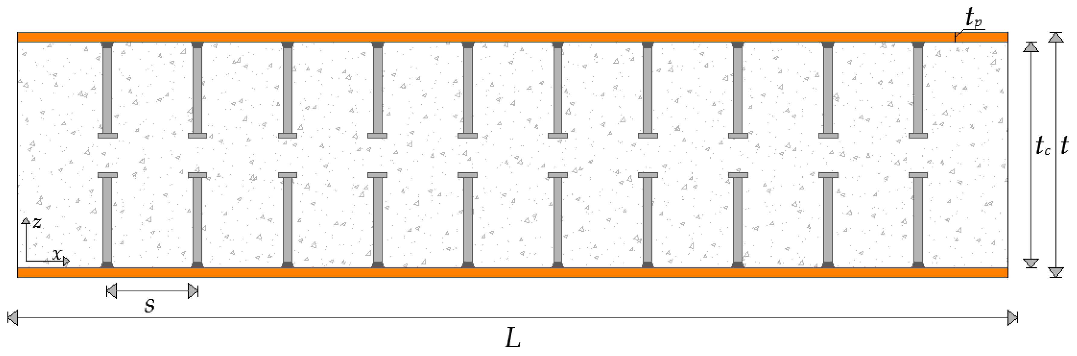
Figure 3.
The concrete stress-strain model.
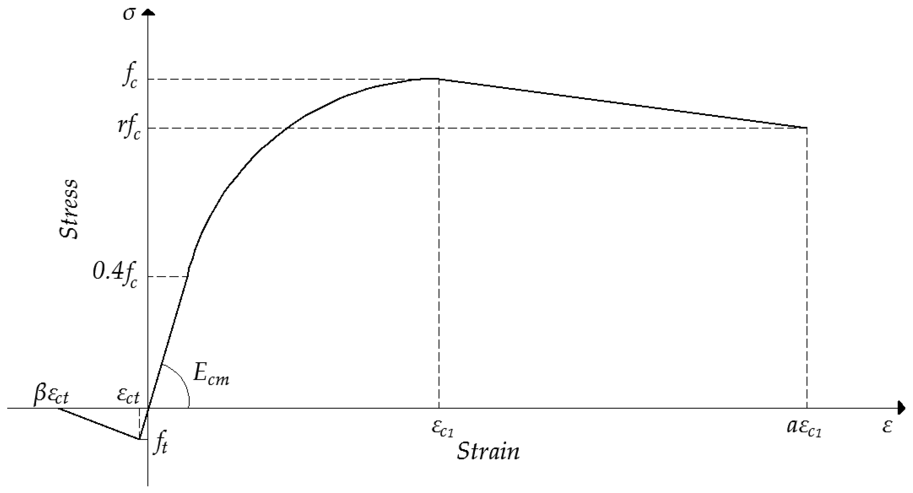
Figure 4.
The steel stress-strain model.
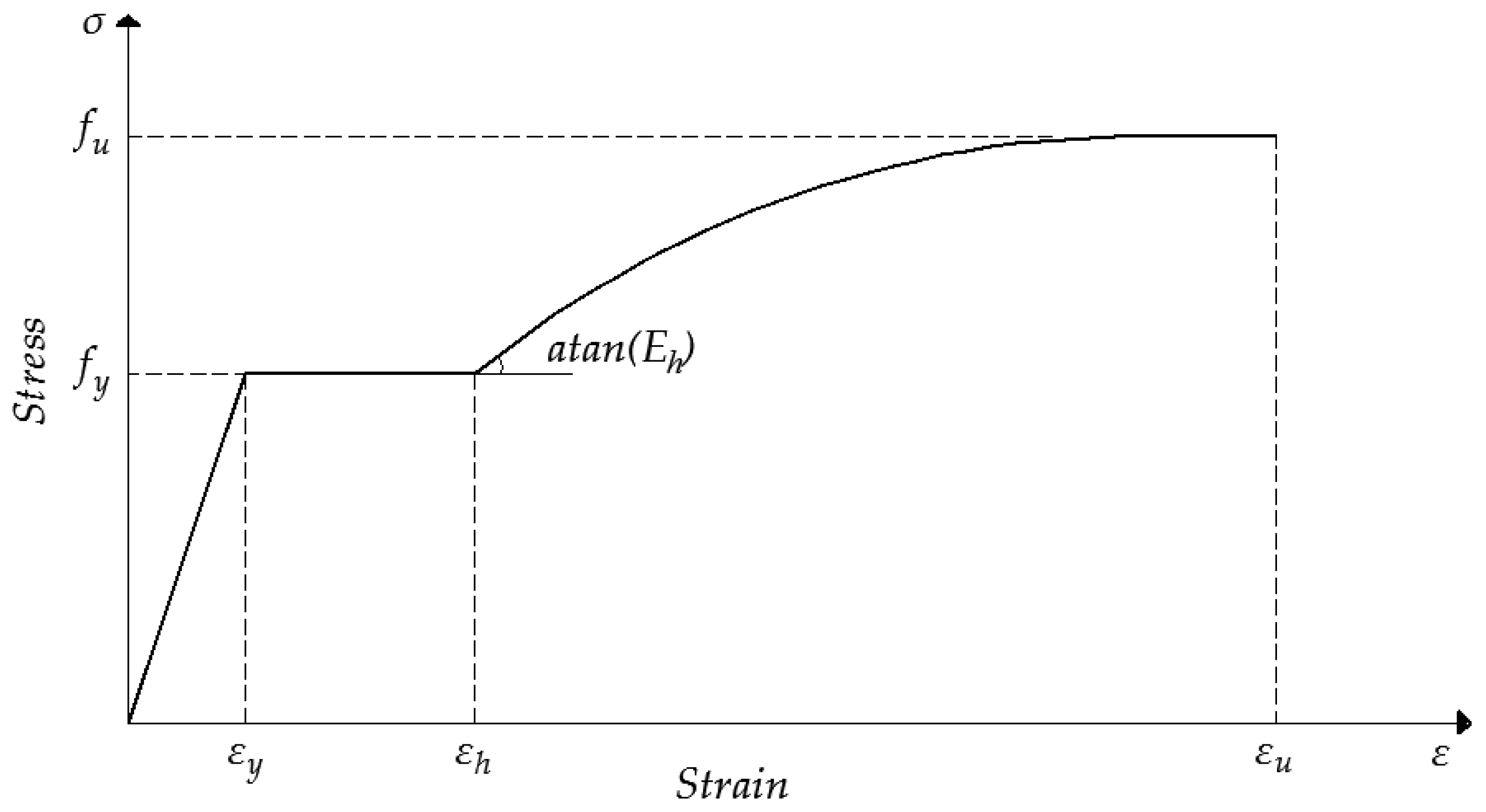
Figure 5.
Cyclic behaviour of steel.

Figure 6.
Calculation of the parameter .

Figure 7.
Finite element modelling of shear connectors.

Figure 8.
Computational model finite element grid, loading and support conditions (a) Detailed model; (b) Simplified model.
Figure 8.
Computational model finite element grid, loading and support conditions (a) Detailed model; (b) Simplified model.

Figure 9.
Computational model finite element grid, loading and support conditions (a) Mesh A (b) Mesh B (c) Mesh C.
Figure 9.
Computational model finite element grid, loading and support conditions (a) Mesh A (b) Mesh B (c) Mesh C.

Figure 10.
Example of Newton-Raphson Solution (a) First Iteration (b) Next Iteration.
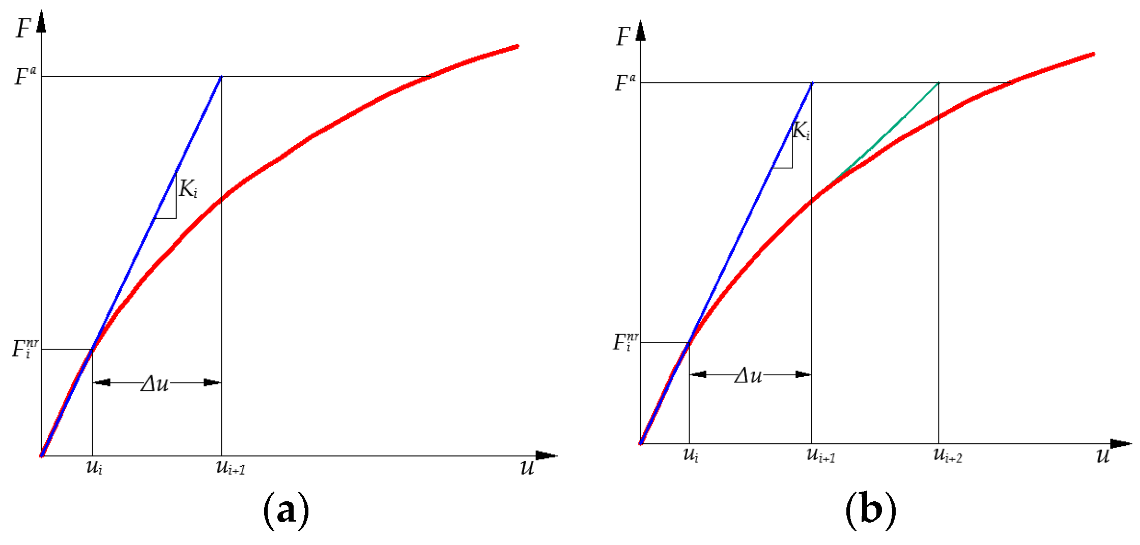
Figure 11.
In-plane shear force—Lateral displacement Curves of SC1.
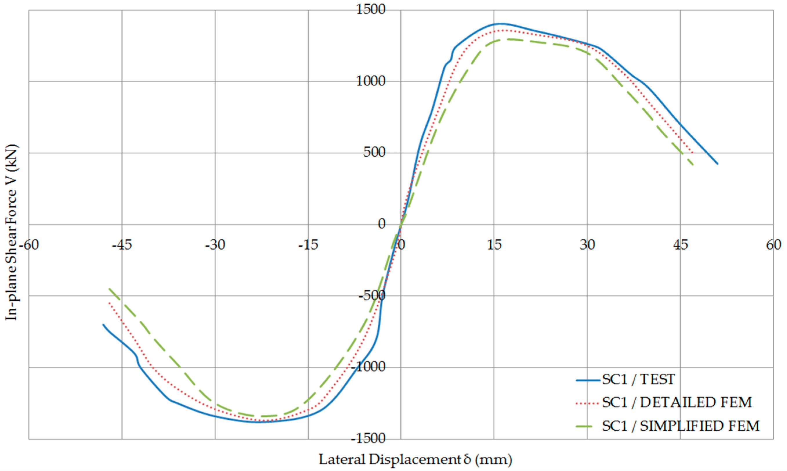
Figure 12.
In-plane shear force—Lateral displacement Curves of SC4.
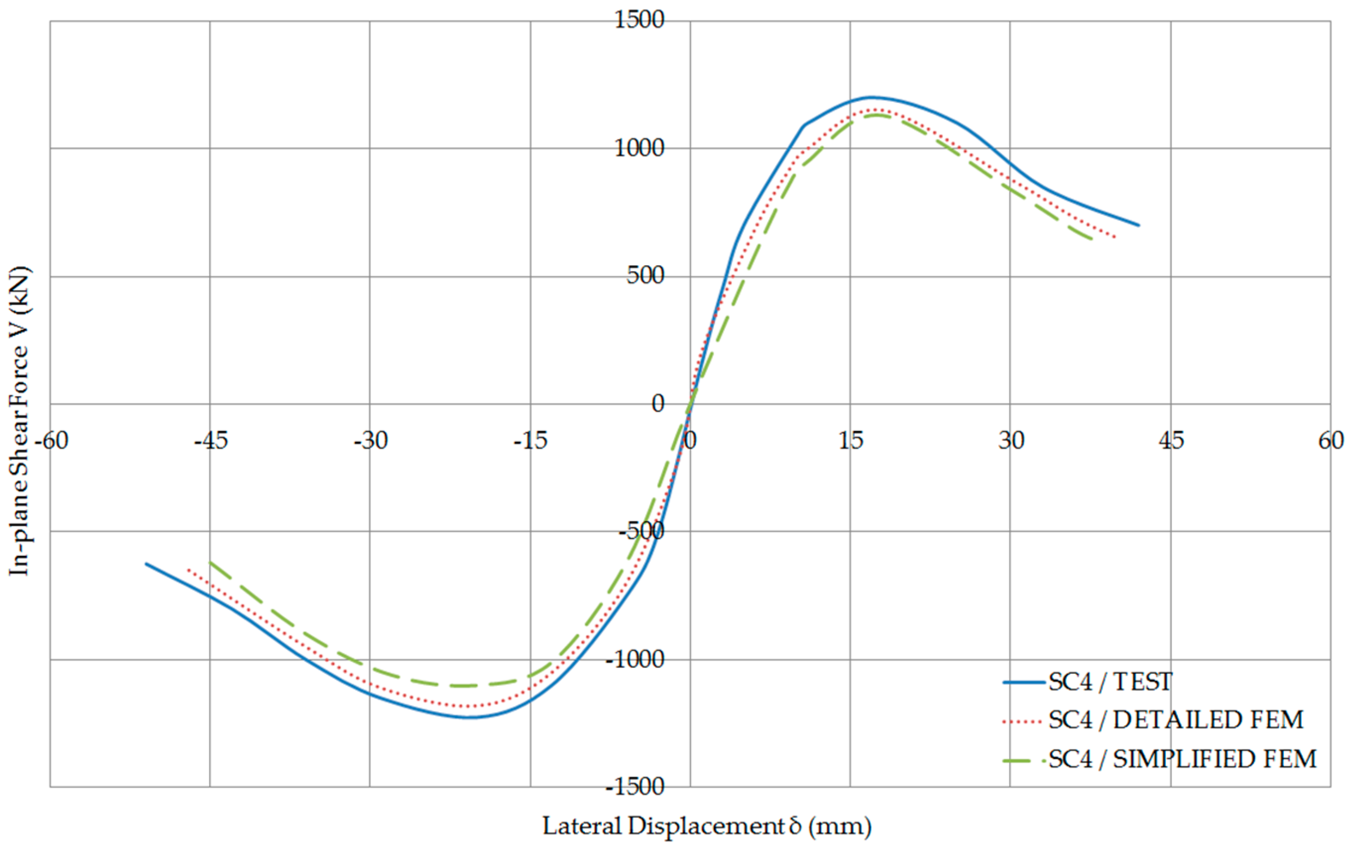
Figure 13.
(a) Out-of-plane displacement (mm) of the analysed specimen SC4; (b) Failure mode of analysed specimen SC4—Distribution of Von Mises stresses (MPa) at the right toe of the wall.
Figure 13.
(a) Out-of-plane displacement (mm) of the analysed specimen SC4; (b) Failure mode of analysed specimen SC4—Distribution of Von Mises stresses (MPa) at the right toe of the wall.

Figure 14.
In-plane shear force—Shear strain Curves of S2-00-NN.

Figure 15.
In-plane shear force—Shear strain Curves of S3-00-NN.

Figure 16.
In-plane shear force—Shear strain Curves of S2-15-NN.

Figure 17.
In-plane shear force—Shear strain Curves of S2-30-NN.

Figure 18.
Axial force—Shortening Curves of C24/490-T6B20 (Comparison of mesh densities).

Figure 19.
Axial force—Shortening Curves of H16/490-T6B30 (Comparison of mesh densities).

Figure 20.
Axial force—Slip Curves of TS1-0.6 (Comparison of mesh densities).
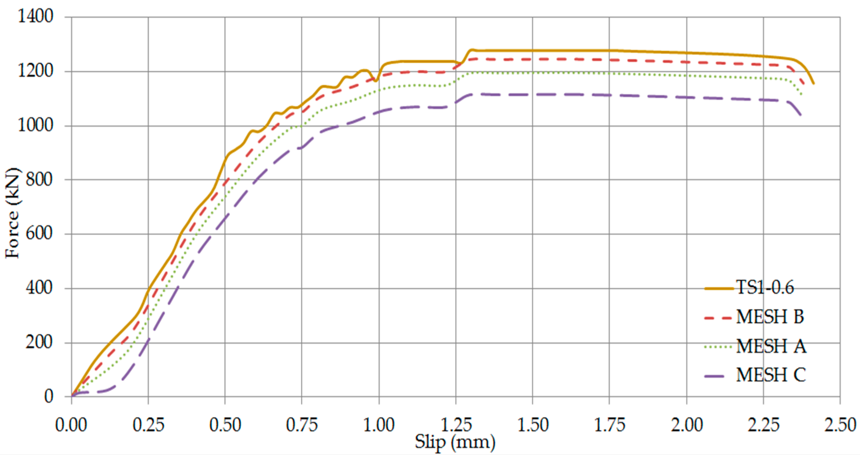
Figure 21.
Axial force—Slip Curves of TS1-1.2 (Comparison of mesh densities).

Figure 22.
Axial force—Slip Curves of TS2-0.6 (Comparison of mesh densities).
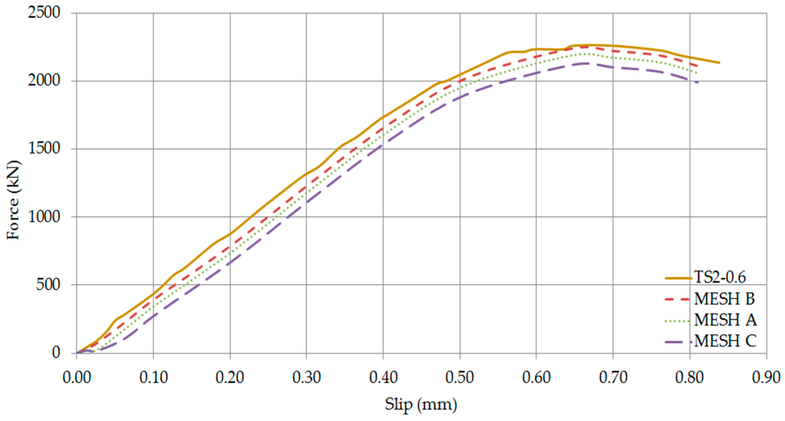
Figure 23.
Axial force—Slip Curves of TS2-1.0 (Comparison of mesh densities).

Figure 24.
Axial force—Slip Curves of TS1-0.6 (Comparison of friction coefficients).
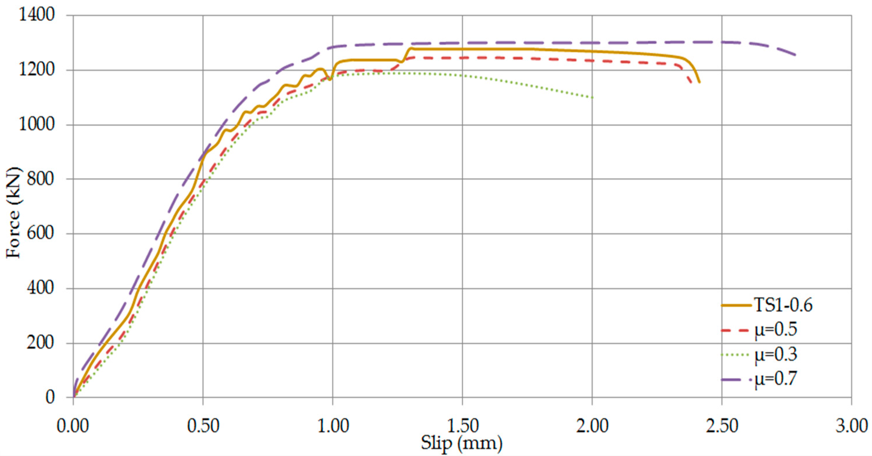
Figure 25.
Axial force—Slip Curves of TS1-1.2 (Comparison of friction coefficients).
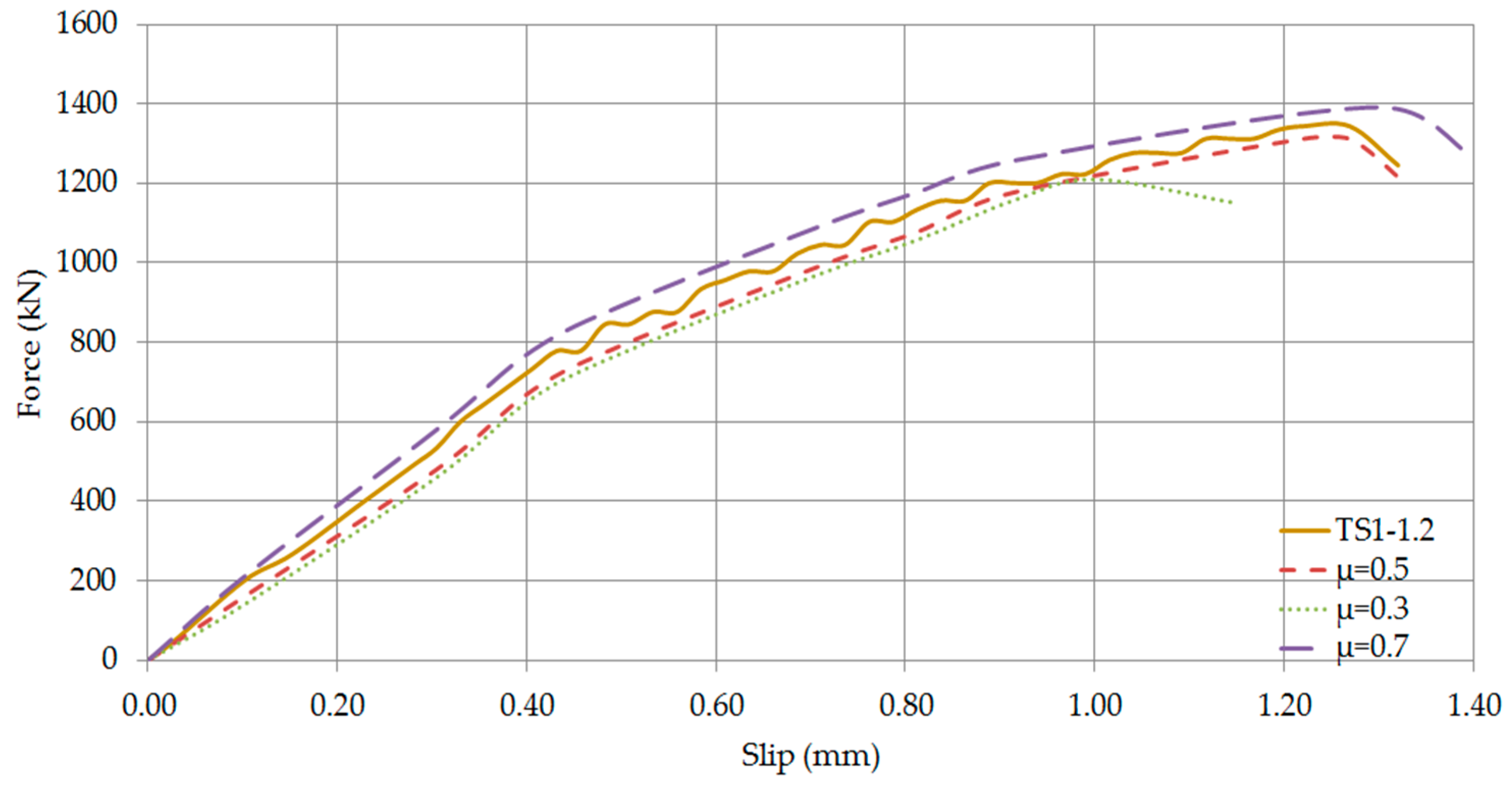
Figure 26.
Axial force—Slip Curves of TS2-0.6 (Comparison of friction coefficients).

Figure 27.
Axial force—Slip Curves of TS2-1.0 (Comparison of friction coefficients).

Figure 28.
Cyclic loading protocol of specimen AE1.


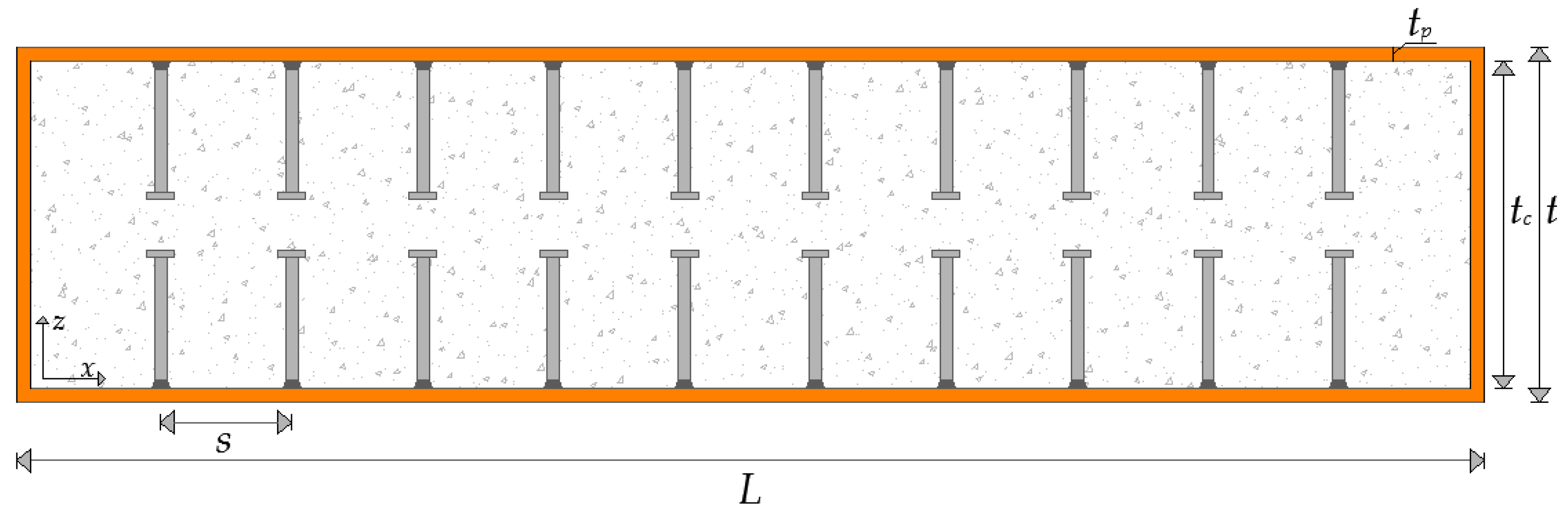
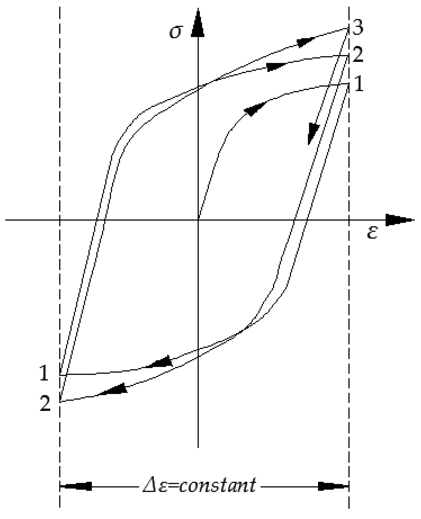
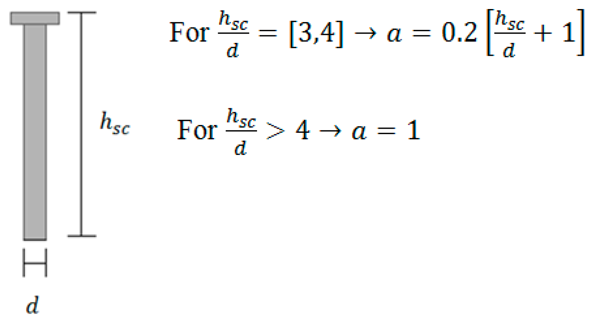
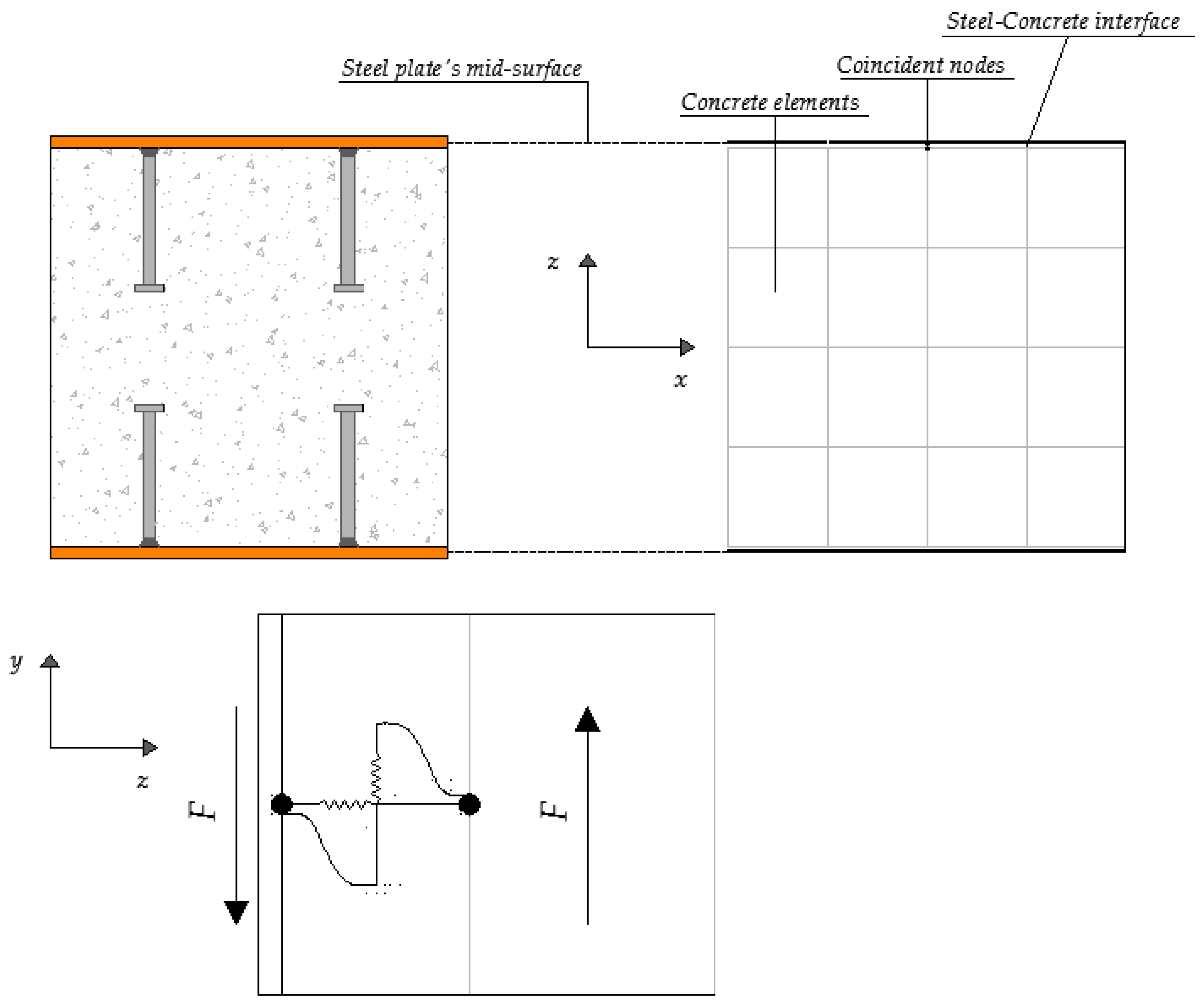
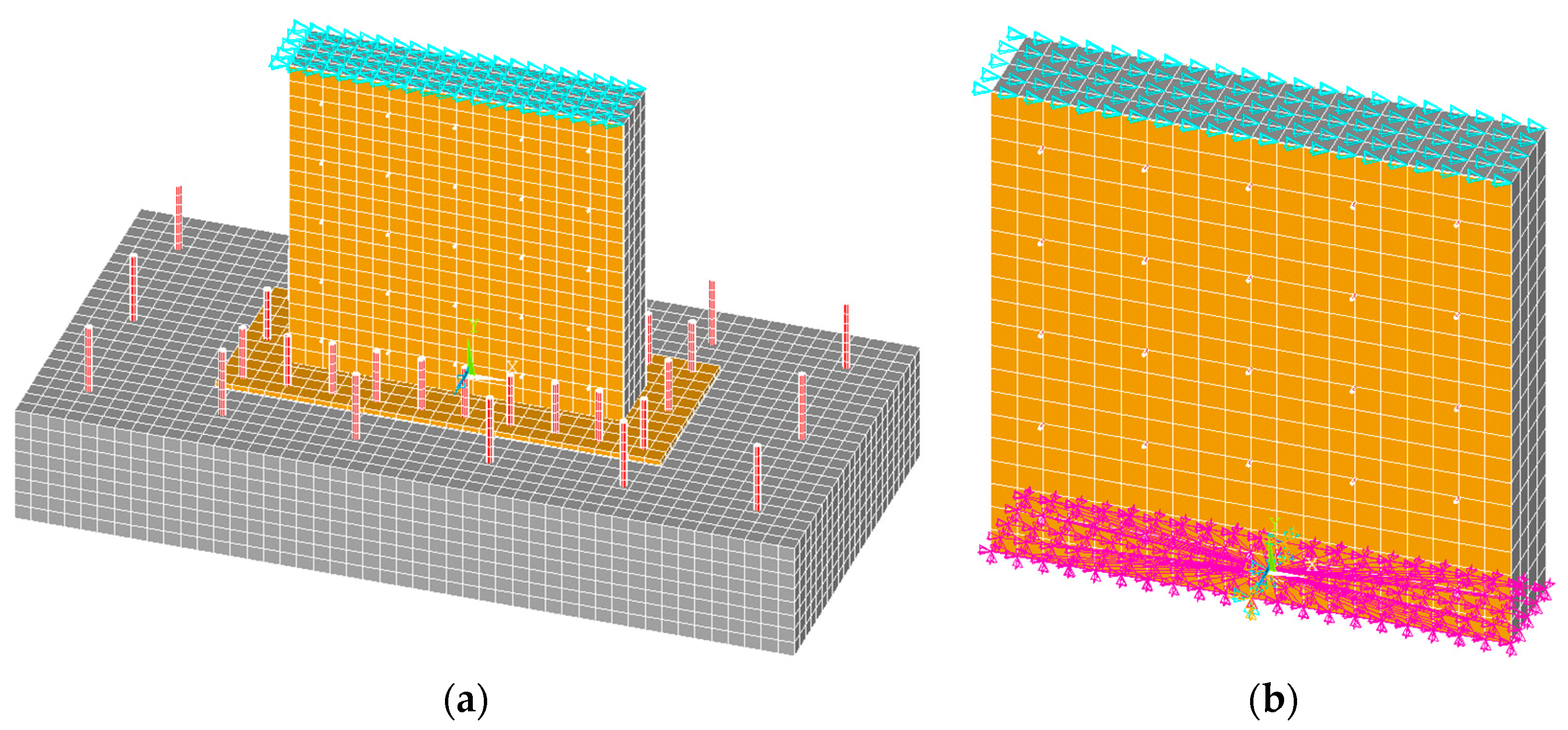
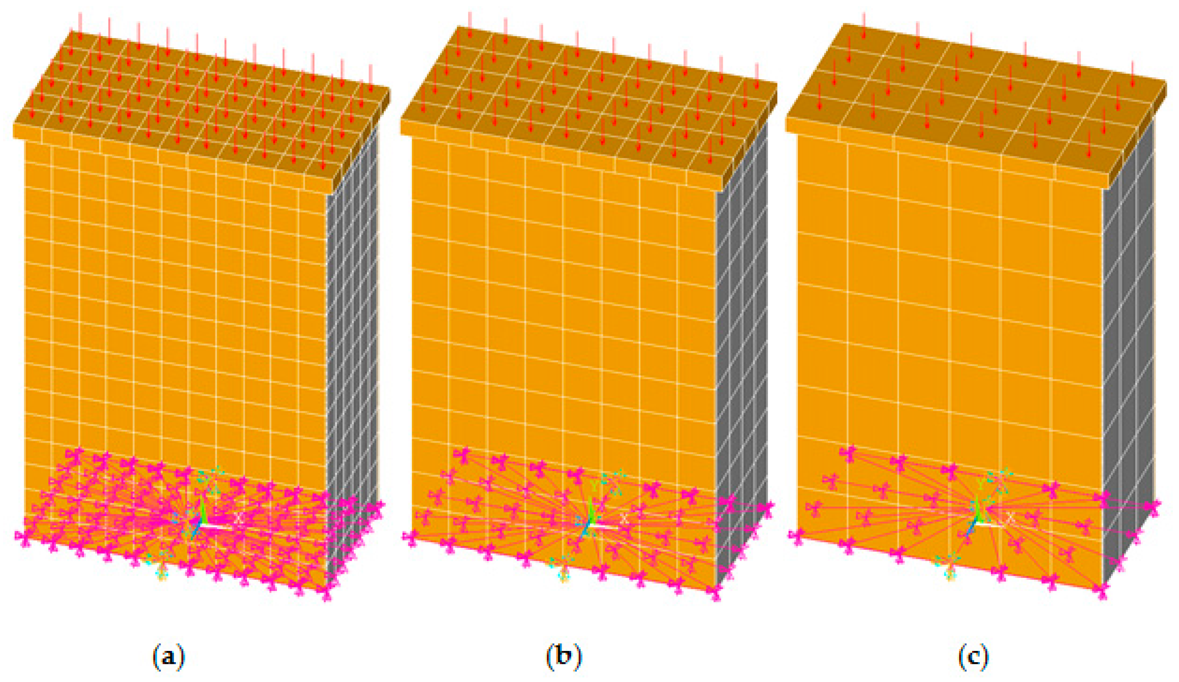
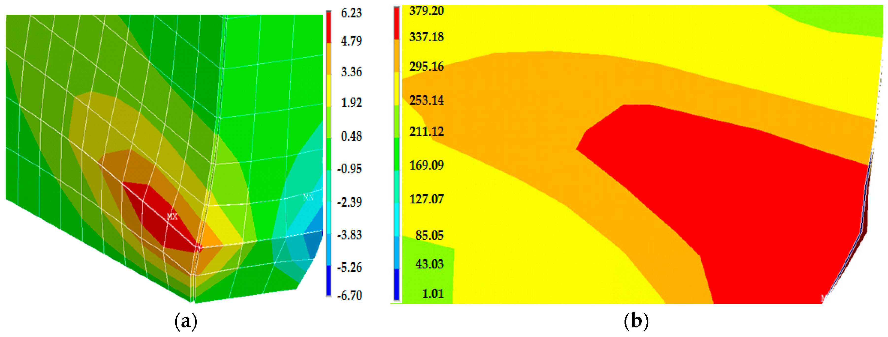
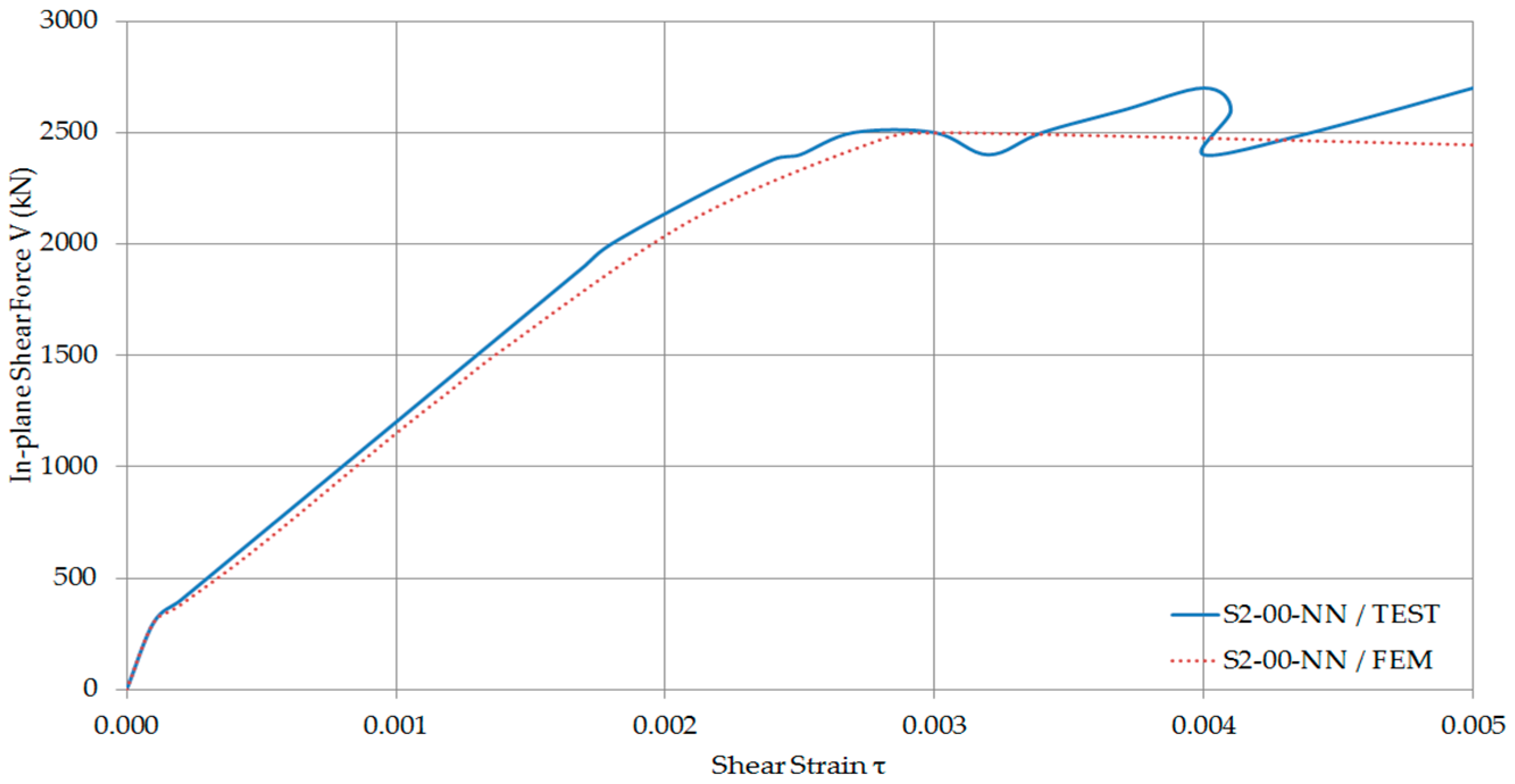
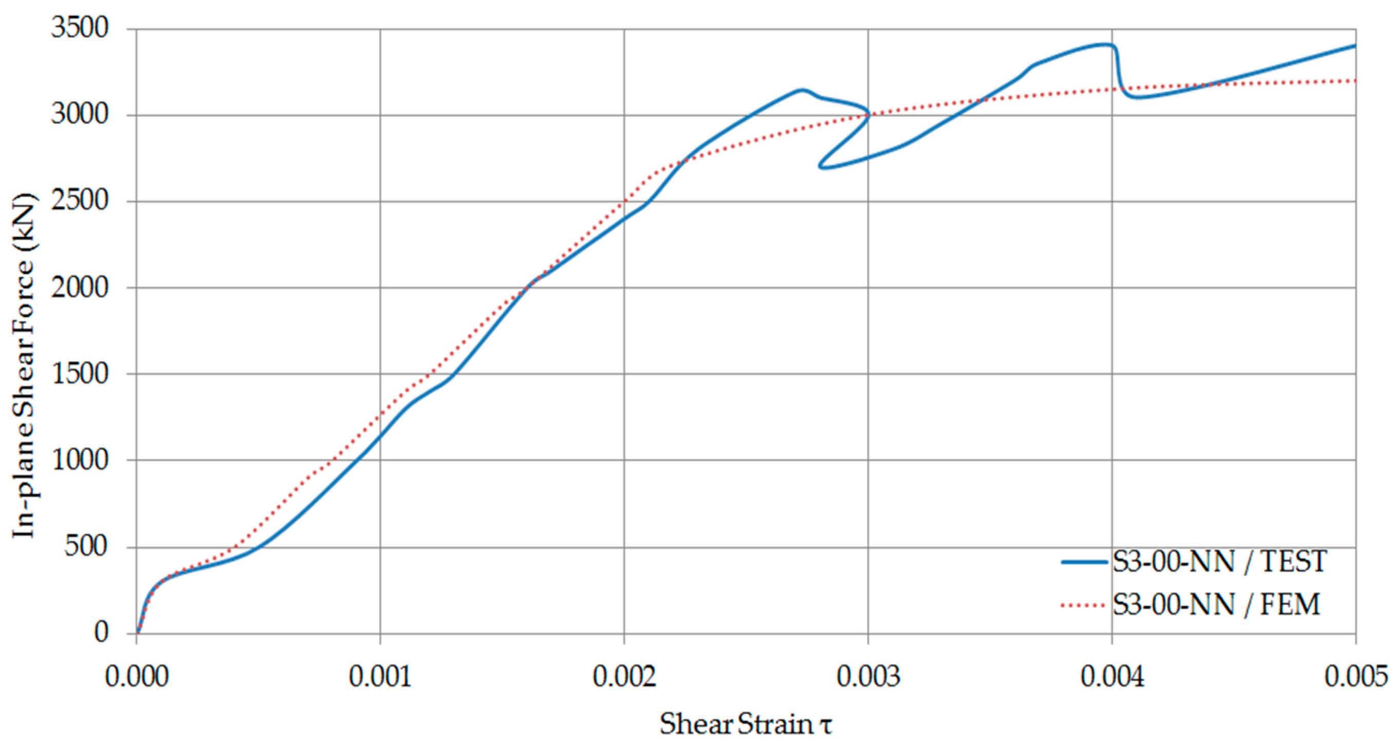
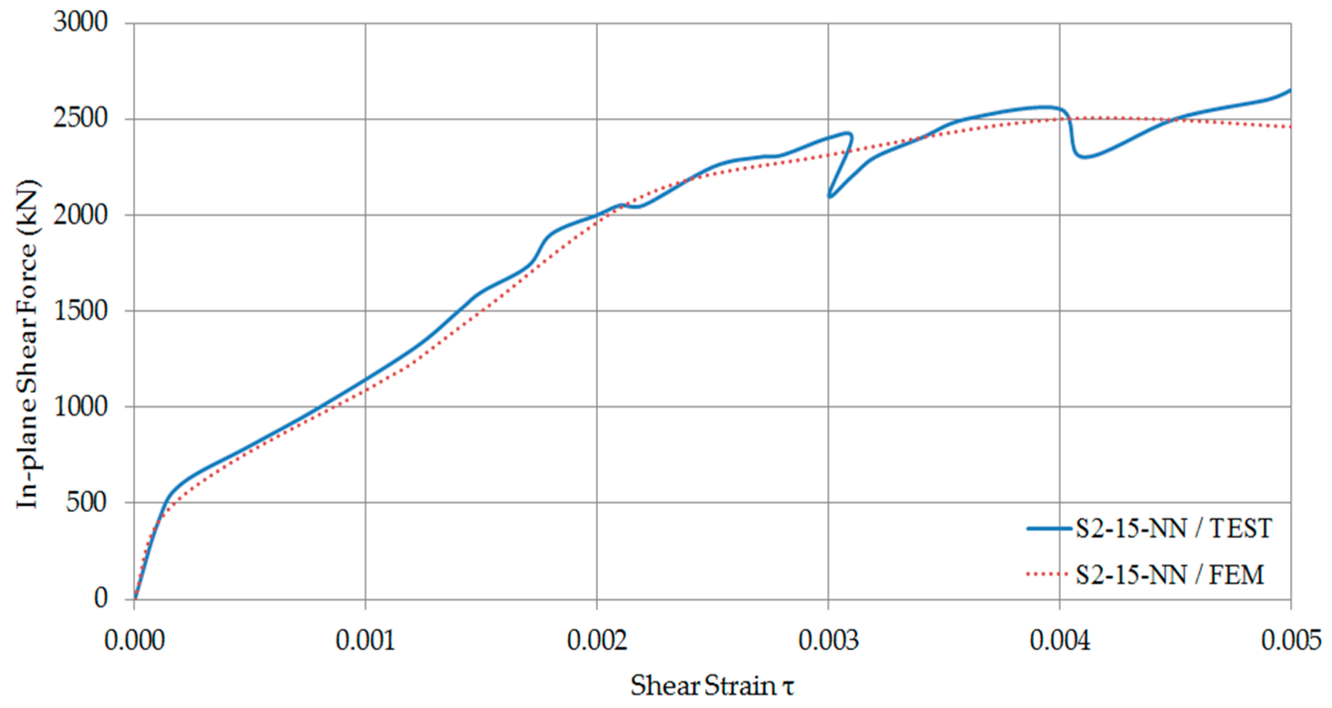
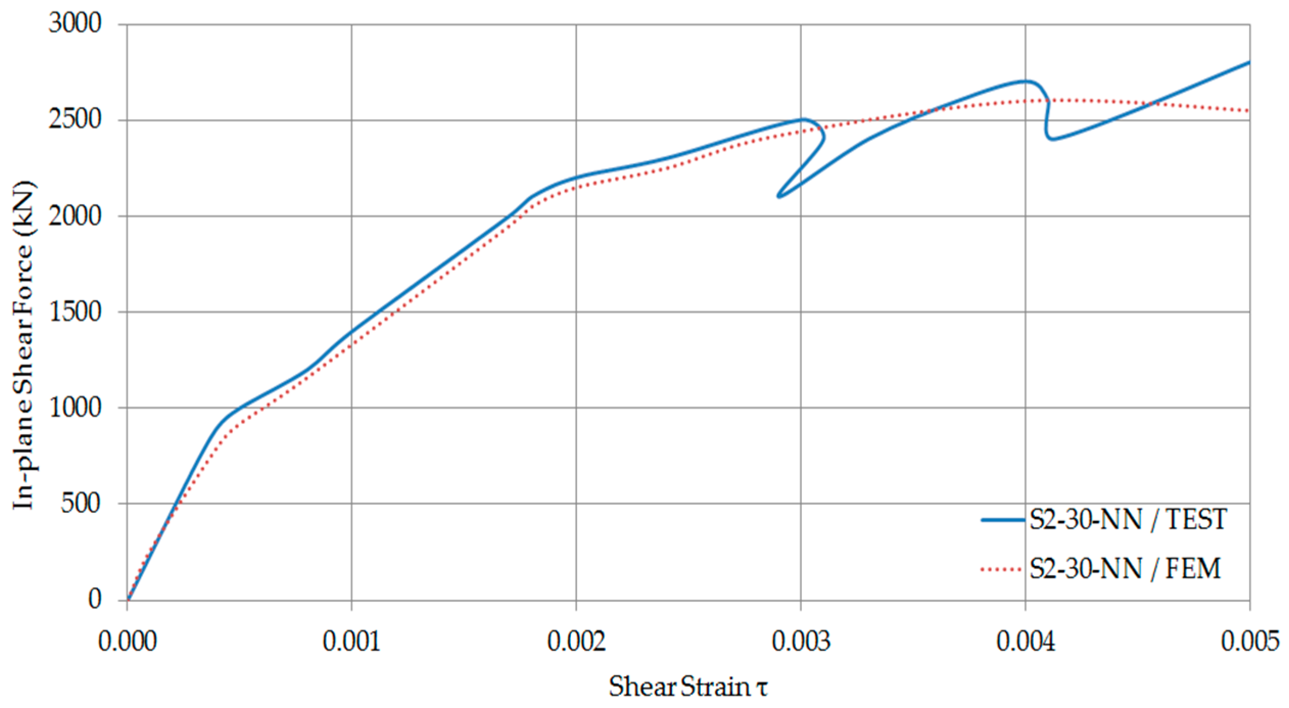
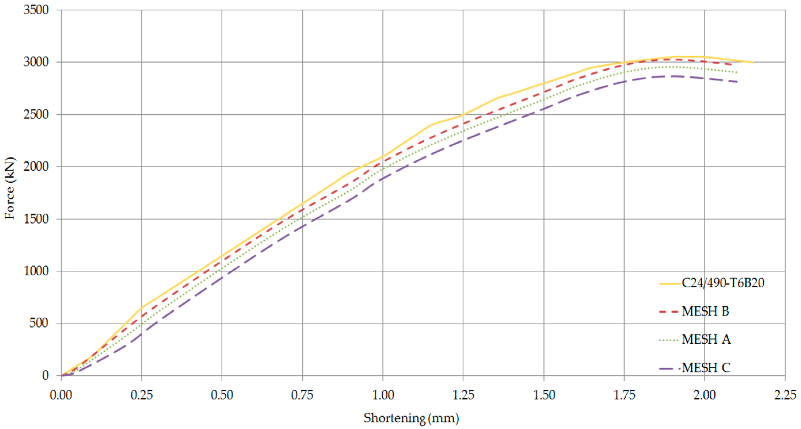
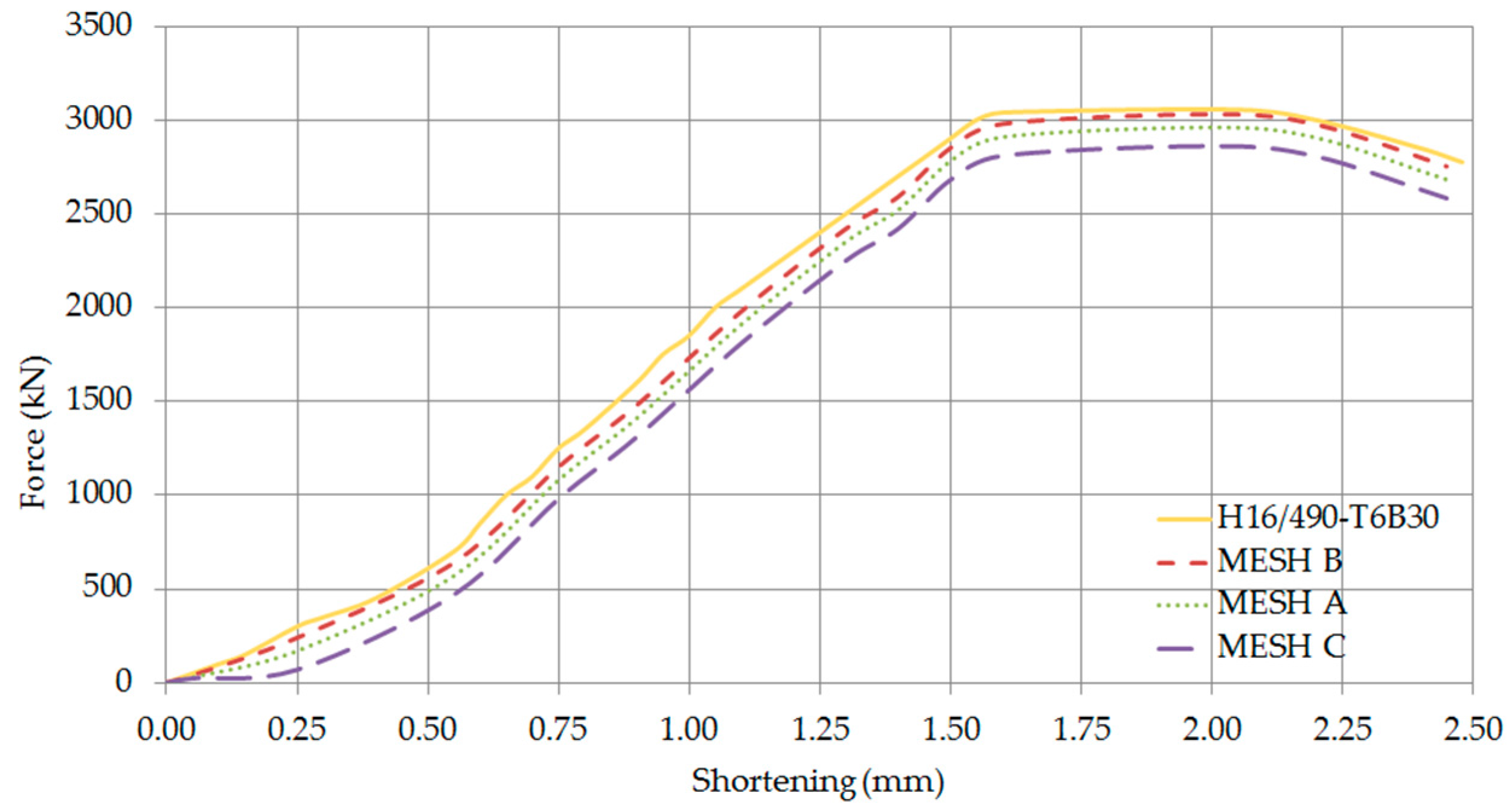
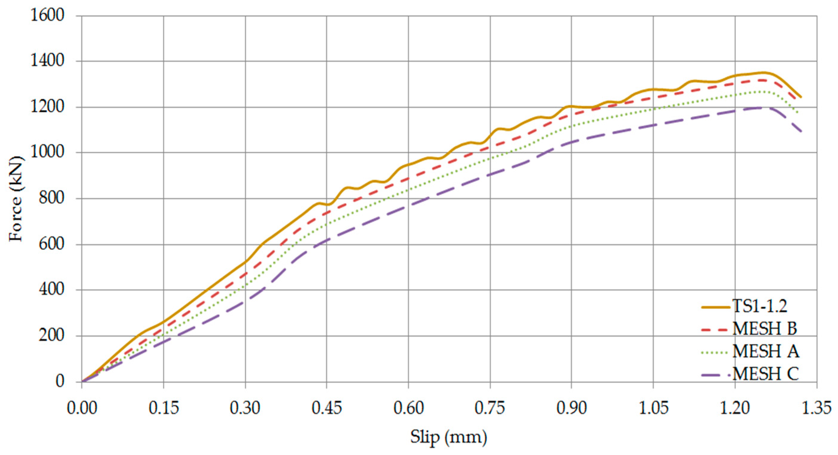
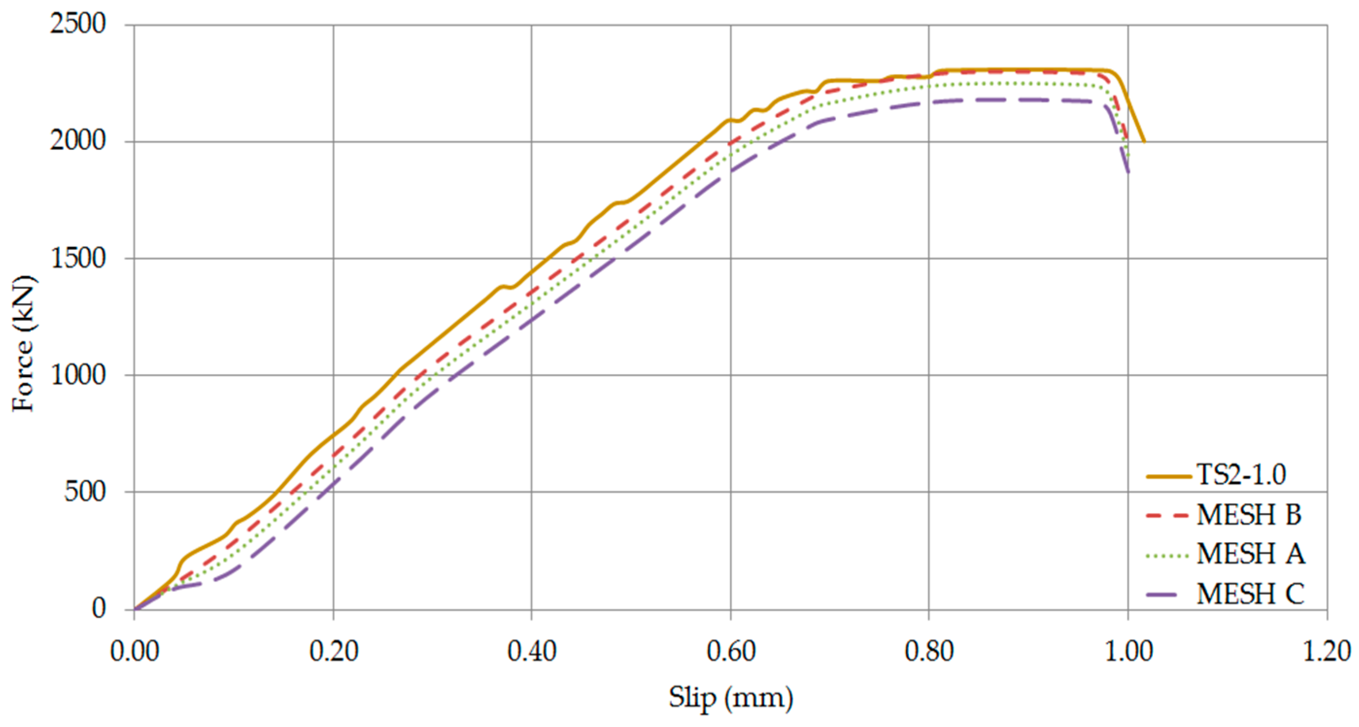
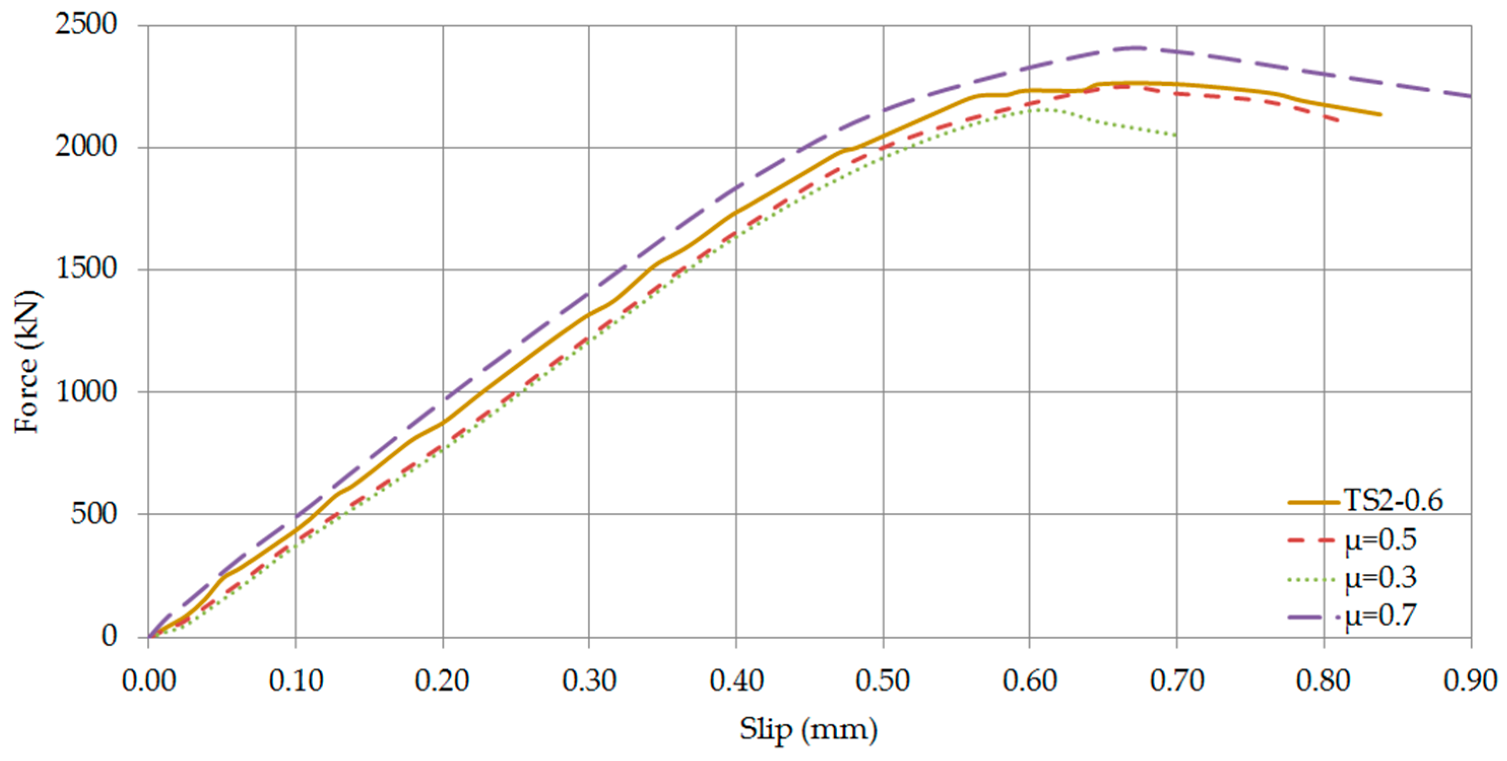
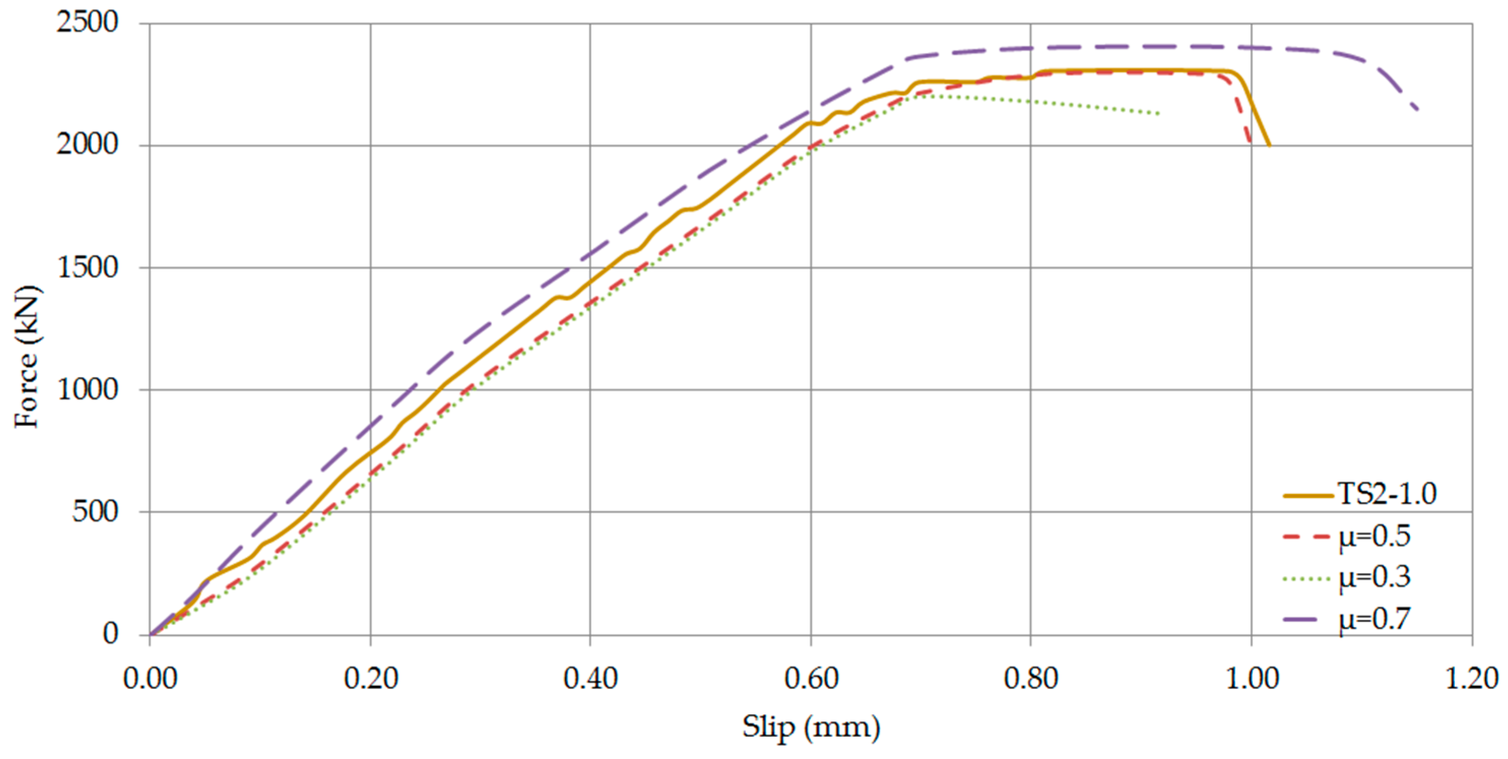
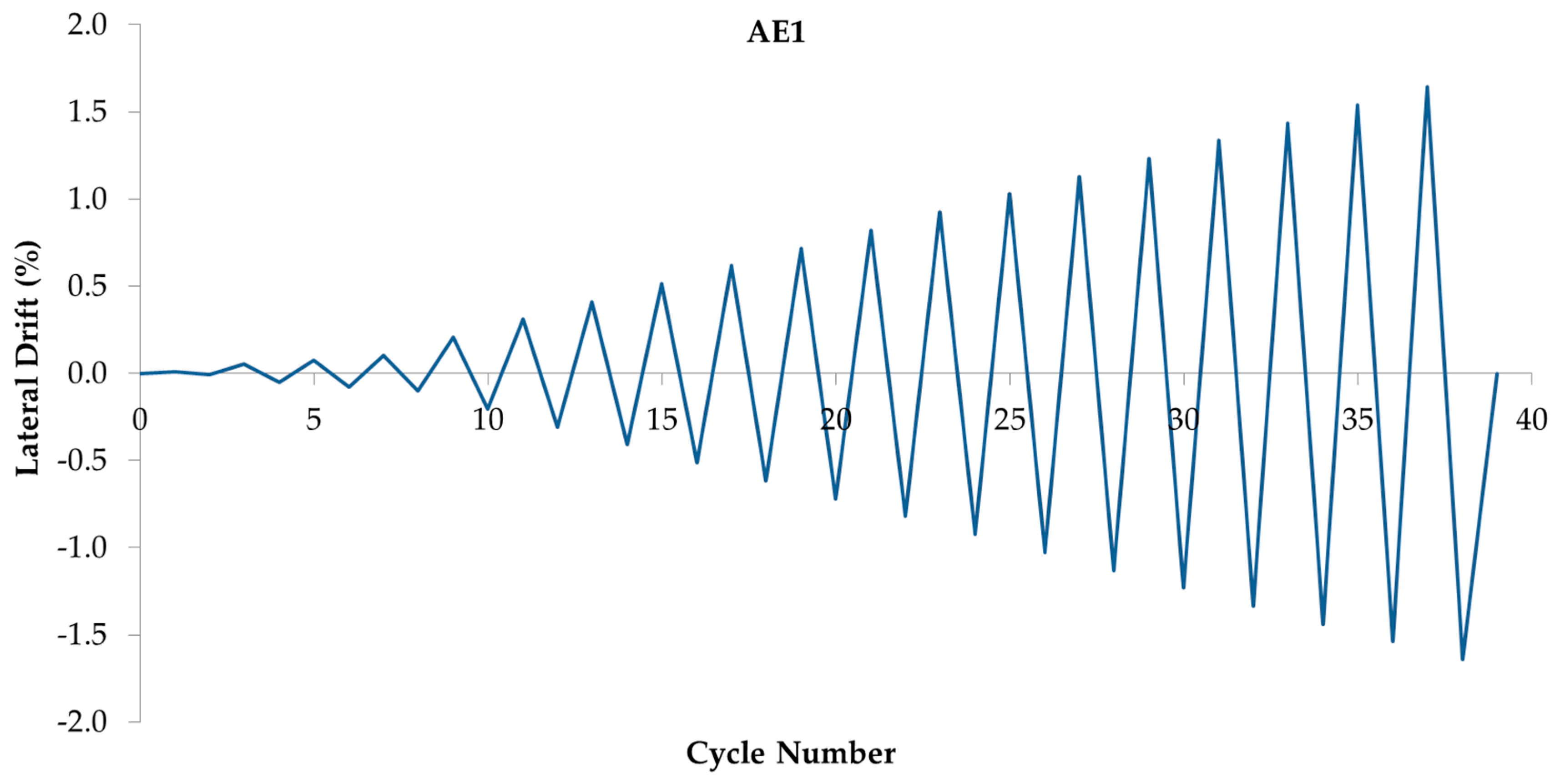
| Loading | Specimen | H | L | t | tp | sx | sy | b | Slenderness | fy | fc |
|---|---|---|---|---|---|---|---|---|---|---|---|
| mm | mm | mm | mm | mm | mm | mm | MPa | MPa | |||
| Axial Compression | NS50 | 960 | 960 | 246.4 | 3.2 | 160.0 | 160.0 | - | 50.0 | 299.1 | 23.5 |
| NS75 | 960 | 960 | 246.4 | 3.2 | 240.0 | 240.0 | - | 75.0 | 299.1 | 23.5 | |
| NS100 | 1280 | 960 | 246.4 | 3.2 | 320.0 | 320.0 | - | 100.0 | 299.1 | 23.5 | |
| NS20 | 640 | 640 | 200.0 | 3.2 | 65.0 | 65.0 | - | 20.0 | 287.0 | 31.2 | |
| NS30 | 640 | 640 | 200.0 | 3.2 | 97.0 | 97.0 | - | 30.0 | 287.0 | 31.2 | |
| NS40 | 640 | 640 | 200.0 | 3.2 | 130.0 | 130.0 | - | 40.0 | 287.0 | 31.2 | |
| NS50 | 640 | 640 | 200.0 | 3.2 | 162.0 | 162.0 | - | 50.0 | 287.0 | 31.2 | |
| C24/490-T6B20 | 380 | 280 | 250.0 | 6.0 | 90.0 | 120.0 | - | 20.0 | 428.5 | 24.0 | |
| C24/490-T6B30 | 500 | 370 | 250.0 | 6.0 | 135.0 | 180.0 | - | 30.0 | 428.5 | 24.0 | |
| C24/490-T6B40 | 620 | 460 | 250.0 | 6.0 | 180.0 | 240.0 | - | 40.0 | 428.5 | 24.0 | |
| H16/490-T6B20 | 380 | 280 | 250.0 | 6.0 | 90.0 | 120.0 | - | 20.0 | 428.5 | 16.0 | |
| H16/490-T6B30 | 500 | 370 | 250.0 | 6.0 | 135.0 | 180.0 | - | 30.0 | 428.5 | 16.0 | |
| H16/490-T6B40 | 620 | 460 | 250.0 | 6.0 | 180.0 | 240.0 | - | 40.0 | 428.5 | 16.0 | |
| TS1-0.6 | 490 | 280 | 139.7 | 4.7 | 70.0 | 70.0 | - | 15.0 | 275.0 | 16.0 | |
| TS1-0.8 | 552 | 276 | 137.2 | 4.7 | 92.0 | 92.0 | - | 19.7 | 275.0 | 16.0 | |
| TS1-1.2 | 560 | 280 | 152.4 | 4.7 | 140.0 | 140.0 | - | 30.0 | 275.0 | 16.0 | |
| TS1-1.4 | 486 | 324 | 146.1 | 4.7 | 162.0 | 162.0 | - | 34.7 | 275.0 | 16.0 | |
| TS1-1.6 | 552 | 368 | 146.1 | 4.7 | 184.0 | 184.0 | - | 39.4 | 275.0 | 16.0 | |
| TS2-0.6 | 495 | 330 | 174.9 | 4.9 | 82.6 | 82.6 | - | 16.9 | 259.2 | 30.3 | |
| TS2-0.8 | 495 | 330 | 174.9 | 4.9 | 111.1 | 111.1 | - | 22.7 | 259.2 | 30.3 | |
| TS2-1.0 | 495 | 330 | 174.9 | 4.9 | 136.5 | 136.5 | - | 27.9 | 259.2 | 32.2 | |
| TS2-1.2 | 495 | 330 | 174.9 | 4.9 | 165.1 | 165.1 | - | 33.7 | 259.2 | 32.2 | |
| Shear& Axial | S2-15-NN | 1200 | 1200 | 200.0 | 2.3 | 70.0 | 70.0 | - | 30.4 | 340.0 | 41.6 |
| S2-30-NN | 1200 | 1200 | 200.0 | 2.3 | 70.0 | 70.0 | - | 30.4 | 340.0 | 42.0 | |
| S3-15-NN | 1200 | 1200 | 200.0 | 3.2 | 100.0 | 100.0 | - | 31.3 | 351.0 | 41.6 | |
| S3-30-NN | 1200 | 1200 | 200.0 | 3.2 | 100.0 | 100.0 | - | 31.3 | 351.0 | 40.1 | |
| In-plane Shear | S2-00-NN | 1200 | 1200 | 200.0 | 2.3 | 70.0 | 70.0 | - | 30.4 | 340.0 | 42.2 |
| S3-00-NN | 1200 | 1200 | 200.0 | 3.2 | 100.0 | 100.0 | - | 31.3 | 351.0 | 41.9 | |
| S4-00-NN | 1200 | 1200 | 200.0 | 4.5 | 135.0 | 135.0 | - | 30.0 | 346.0 | 42.8 | |
| SC1 | 1524 | 1524 | 305.0 | 4.8 | 102.0 | 102.0 | 305.0 | 21.3 | 262.0 | 30.3 | |
| SC2 | 1524 | 1524 | 305.0 | 4.8 | - | - | 152.0 | 31.7 | 262.0 | 30.3 | |
| SC3 | 1524 | 1524 | 229.0 | 4.8 | 114.0 | 114.0 | 229.0 | 23.8 | 262.0 | 36.5 | |
| SC4 | 1524 | 1524 | 229.0 | 4.8 | - | - | 114.0 | 23.8 | 262.0 | 36.5 |
| Specimen | Results | Py | Pu | δy | δu | Failure Mode |
|---|---|---|---|---|---|---|
| (kN) | (kN) | (mm) | (mm) | |||
| NS50 | Test | 5884.0 | 7256.9 | 1.88 | 4.25 | (a) buckling of surface plates (b) yielding of side plates (c) ultimate strength (d) rapid loss of load carrying capacity |
| ANSYS | 5852.2 | 7132.1 | 1.85 | 4.08 | ||
| Error% | 0.54 | 1.72 | 1.60 | 4.00 | ||
| NS75 | Test | 5001.4 | 7011.8 | 1.5 | 3.5 | |
| ANSYS | 4976.5 | 6915.3 | 1.48 | 3.43 | ||
| Error% | 0.50 | 1.38 | 1.33 | 2.00 | ||
| NS100 | Test | 5393.7 | 7364.8 | 2.38 | 4.63 | |
| ANSYS | 5371.2 | 7245.1 | 2.35 | 4.59 | ||
| Error% | 0.42 | 1.63 | 1.26 | 0.86 | ||
| NS20 | Test | 3210.0 | 5730.2 | 0.7 | 2.58 | extensive local buckling & concrete crushing |
| ANSYS | 3189.3 | 5620.1 | 0.66 | 2.41 | ||
| Error% | 0.64 | 1.92 | 5.71 | 6.59 | ||
| NS30 | Test | 4710.0 | 5470.0 | 2.17 | 3.28 | |
| ANSYS | 4683.3 | 5392.1 | 2.14 | 3.16 | ||
| Error% | 0.57 | 1.42 | 1.38 | 3.66 | ||
| NS40 | Test | 4940.0 | 4999.8 | 3.3 | 3.65 | |
| ANSYS | 4916.3 | 4879.9 | 3.26 | 3.58 | ||
| Error% | 0.48 | 2.40 | 1.21 | 1.92 | ||
| NS50 | Test | 4120.0 | 5050.0 | 3.2 | 4.18 | |
| ANSYS | 4101.1 | 4945.9 | 3.19 | 4.11 | ||
| Error% | 0.46 | 2.06 | 0.31 | 1.67 |
| Specimen | Variables | ||||||
|---|---|---|---|---|---|---|---|
| H (mm) | t (mm) | tp (mm) | fy (MPa) | fc (MPa) | Aspect Ratio (H/L) | Reinf. Ratio (%) | |
| AE1 | 1500 | 200 | 4 | 235 | 30 | 0.75 | 4.6 |
| AE2 | 1500 | 200 | 4 | 235 | 40 | 0.75 | 4.6 |
| AE3 | 1500 | 200 | 4 | 355 | 30 | 0.75 | 4.6 |
| AE4 | 1500 | 200 | 4 | 355 | 40 | 0.75 | 4.6 |
| AE5 | 1500 | 200 | 8 | 235 | 30 | 0.75 | 9.6 |
| AE6 | 1500 | 200 | 8 | 235 | 40 | 0.75 | 9.6 |
| AE7 | 1500 | 200 | 8 | 355 | 30 | 0.75 | 9.6 |
| AE8 | 1500 | 200 | 8 | 355 | 40 | 0.75 | 9.6 |
| AE9 | 4000 | 200 | 4 | 235 | 30 | 2.0 | 4.6 |
| AE10 | 4000 | 200 | 4 | 235 | 40 | 2.0 | 4.6 |
| AE11 | 4000 | 200 | 4 | 355 | 30 | 2.0 | 4.6 |
| AE12 | 4000 | 200 | 4 | 355 | 40 | 2.0 | 4.6 |
| AE13 | 4000 | 200 | 8 | 235 | 30 | 2.0 | 9.6 |
| AE14 | 4000 | 200 | 8 | 235 | 40 | 2.0 | 9.6 |
| AE15 | 4000 | 200 | 8 | 355 | 30 | 2.0 | 9.6 |
| AE16 | 4000 | 200 | 8 | 355 | 40 | 2.0 | 9.6 |
| Specimen | Yielding Point | Ultimate Point | Failure Point | ||||||
|---|---|---|---|---|---|---|---|---|---|
| Vy (kN) | δy (mm) | dy (%) | Vu (kN) | δu (mm) | du (%) | Vuf (kN) | δf (mm) | df (%) | |
| AE1 | 1192.1 | 1.54 | 0.103 | 2286.4 | 4.68 | 0.31 | 1829.1 | 21.60 | 1.44 |
| AE2 | 1659.2 | 1.02 | 0.068 | 2851.3 | 5.04 | 0.34 | 2281.0 | 21.90 | 1.46 |
| AE3 | 2197.4 | 2.24 | 0.149 | 3305.0 | 6.30 | 0.42 | 2644.0 | 20.55 | 1.37 |
| AE4 | 2717.9 | 2.05 | 0.136 | 4261.4 | 6.66 | 0.44 | 3409.1 | 21.15 | 1.41 |
| AE5 | 2023.9 | 1.03 | 0.069 | 4225.8 | 4.91 | 0.33 | 3380.6 | 20.40 | 1.36 |
| AE6 | 2571.1 | 1.38 | 0.092 | 5386.8 | 6.35 | 0.42 | 4309.4 | 20.70 | 1.38 |
| AE7 | 3345.0 | 2.70 | 0.180 | 7219.4 | 7.86 | 0.52 | 5775.5 | 19.35 | 1.29 |
| AE8 | 3727.6 | 2.40 | 0.160 | 8233.6 | 7.77 | 0.52 | 6586.9 | 19.95 | 1.33 |
| AE9 | 306.9 | 3.07 | 0.077 | 507.1 | 35.17 | 0.88 | 405.7 | 73.20 | 1.83 |
| AE10 | 385.8 | 2.99 | 0.075 | 564.9 | 39.99 | 1.00 | 451.9 | 76.80 | 1.92 |
| AE11 | 431.5 | 9.13 | 0.228 | 965.3 | 51.19 | 1.28 | 772.2 | 70.40 | 1.76 |
| AE12 | 507.1 | 7.12 | 0.178 | 1045.3 | 52.06 | 1.30 | 836.3 | 75.20 | 1.88 |
| AE13 | 533.8 | 6.00 | 0.150 | 1174.3 | 40.86 | 1.02 | 939.5 | 70.00 | 1.75 |
| AE14 | 649.4 | 5.74 | 0.143 | 1290.0 | 49.00 | 1.22 | 1032.0 | 73.60 | 1.84 |
| AE15 | 840.7 | 11.62 | 0.290 | 2157.4 | 71.65 | 1.79 | 1725.9 | 67.20 | 1.68 |
| AE16 | 916.3 | 10.54 | 0.264 | 2410.9 | 71.38 | 1.78 | 1928.7 | 72.00 | 1.80 |
| Specimen | Yielding Point | Ultimate Point | Failure Point | ||||||||
|---|---|---|---|---|---|---|---|---|---|---|---|
| Vy (kN) | δy (mm) | Vu (kN) | δu (mm) | Vuf (kN) | δf (mm) | ||||||
| + | - | + | - | + | - | + | - | + | - | ||
| AE1 | 1222.3 | 1185.6 | 1.54 | 2289.6 | 2175.1 | 4.62 | 4.62 | 1831.7 | 1740.1 | 21.56 | 21.56 |
| AE2 | 1692.9 | 1642.5 | 1.02 | 2854.4 | 2739.4 | 5.10 | 5.10 | 2283.5 | 2191.6 | 21.42 | 21.42 |
| AE3 | 2255.2 | 2188.2 | 2.24 | 3309.7 | 3144.2 | 6.50 | 6.50 | 2647.8 | 2515.4 | 20.10 | 20.10 |
| AE4 | 2775.7 | 2693.2 | 2.05 | 4266.3 | 4095.7 | 6.88 | 6.88 | 3413.1 | 3276.6 | 20.66 | 20.66 |
| AE5 | 2054.9 | 1993.8 | 1.03 | 4231.7 | 4062.4 | 5.03 | 5.01 | 3385.4 | 3250.0 | 20.07 | 20.07 |
| AE6 | 2597.5 | 2520.3 | 1.38 | 5394.3 | 5178.5 | 6.53 | 6.52 | 4315.4 | 4142.8 | 20.34 | 20.34 |
| AE7 | 3399.6 | 3298.5 | 2.70 | 7229.5 | 6940.4 | 8.07 | 8.06 | 5783.6 | 5552.3 | 19.04 | 19.04 |
| AE8 | 3769.7 | 3657.6 | 2.40 | 8245.1 | 7915.3 | 7.98 | 7.98 | 6596.1 | 6332.3 | 19.60 | 19.60 |
| AE9 | 290.0 | 303.8 | 3.07 | 489.9 | 470.3 | 33.77 | 37.15 | 392.9 | 376.2 | 70.61 | 77.67 |
| AE10 | 365.7 | 379.9 | 2.99 | 547.4 | 525.5 | 38.87 | 42.76 | 440.6 | 420.4 | 74.75 | 78.5 |
| AE11 | 407.2 | 426.2 | 9.13 | 934.9 | 897.5 | 50.06 | 55.07 | 748.9 | 718.0 | 68.43 | 70.5 |
| AE12 | 481.1 | 498.9 | 7.12 | 1012.8 | 972.2 | 50.86 | 55.94 | 818.3 | 777.8 | 73.32 | 77.7 |
| AE13 | 511.6 | 529.4 | 6.00 | 1149.2 | 1103.2 | 39.97 | 43.97 | 922.0 | 882.6 | 67.20 | 69.2 |
| AE14 | 622.8 | 643.0 | 5.74 | 1253.3 | 1203.2 | 47.91 | 52.71 | 1005.9 | 962.6 | 70.58 | 76.2 |
| AE15 | 805.7 | 832.2 | 11.62 | 2100.6 | 2016.6 | 70.07 | 77.07 | 1699.6 | 1613.3 | 64.38 | 66.3 |
| AE16 | 876.9 | 906.2 | 10.54 | 2343.2 | 2249.5 | 69.74 | 76.71 | 1890.9 | 1799.6 | 69.12 | 74.6 |
© 2017 by the authors. Licensee MDPI, Basel, Switzerland. This article is an open access article distributed under the terms and conditions of the Creative Commons Attribution (CC BY) license ( http://creativecommons.org/licenses/by/4.0/).
Share and Cite
MDPI and ACS Style
Elmatzoglou, M.; Avdelas, A. Numerical Modelling of Double-Steel Plate Composite Shear Walls. Computation 2017, 5, 12. https://doi.org/10.3390/computation5010012
AMA Style
Elmatzoglou M, Avdelas A. Numerical Modelling of Double-Steel Plate Composite Shear Walls. Computation. 2017; 5(1):12. https://doi.org/10.3390/computation5010012
Chicago/Turabian StyleElmatzoglou, Michaela, and Aris Avdelas. 2017. "Numerical Modelling of Double-Steel Plate Composite Shear Walls" Computation 5, no. 1: 12. https://doi.org/10.3390/computation5010012
Note that from the first issue of 2016, this journal uses article numbers instead of page numbers. See further details here.