Online Adaptive Local-Global Model Reduction for Flows in Heterogeneous Porous Media

Abstract

We propose an online adaptive local-global POD-DEIM model reduction method for flows in heterogeneous porous media. The main idea of the proposed method is to use local online indicators to decide on the global update, which is performed via reduced cost local multiscale basis functions. This unique local-global online combination allows (1) developing local indicators that are used for both local and global updates (2) computing global online modes via local multiscale basis functions. The multiscale basis functions consist of offline and some online local basis functions. The approach used for constructing a global reduced system is based on Proper Orthogonal Decomposition (POD) Galerkin projection. The nonlinearities are approximated by the Discrete Empirical Interpolation Method (DEIM). The online adaption is performed by incorporating new data, which become available at the online stage. Once the criterion for updates is satisfied, we adapt the reduced system online by changing the POD subspace and the DEIM approximation of the nonlinear functions. The main contribution of the paper is that the criterion for adaption and the construction of the global online modes are based on local error indicators and local multiscale basis function which can be cheaply computed. Since the adaption is performed infrequently, the new methodology does not add significant computational overhead associated with when and how to adapt the reduced basis. Our approach is particularly useful for situations where it is desired to solve the reduced system for inputs or controls that result in a solution outside the span of the snapshots generated in the offline stage. Our method also offers an alternative of constructing a robust reduced system even if a potential initial poor choice of snapshots is used. Applications to single-phase and two-phase flow problems demonstrate the efficiency of our method.

1. Introduction

Reduced order models (ROM) aims at reducing the computational complexity and, in turn, the simulation time of large-scale dynamical systems by approximating the state-space to much lower dimensions. This yields reduced models that can produce nearly the same input/output response characteristics as the original ones. Approaches to construct ROMs by projection include the Proper Orthogonal Decomposition (POD) method [1], the balanced truncation (BT) [2], the Krylov subspace projection methods, the trajectory-piecewise linear (TPWL) techniques [3] and variants of them. Among these approaches, the POD method is perhaps the most popular one. For example, the POD was successfully applied to a number of areas [4,5,6,7,8,9,10,11].

For POD projection type model reduction, the process typically consists of an offline stage followed by an online stage. In the offline stage, the low dimension solution space, also called as the POD subspace, is generated and a reduced system for the problem at hand is constructed by projecting onto the low dimension solution space; in the online stage, on the other hand, an approximated solution is obtained by integrating the reduced dynamical system. The online solution relies only on the pre-computed quantities from the offline stage. Therefore, a good approximation from the reduced model can be expected only if the offline information is a good representation of the problem with initial input parameters.

Much progress on adaptivity has been made in the context of model reduction. Offline adaptive methods [12] seek to provide a better reduce solution space while the reduced system is constructed in the offline stage. However, once the reduced system is derived, it stays fixed and is kept unchanged in the online stage. Therefore, the online solution relies only on the pre-computed information from the offline stage which is not incorporated at the online phase. Unlike the offline adaptation, online adaptive methods modify the reduced system during the computations in the integration stage. Most of the existing global online adaptive methods [13,14,15] rely only on precomputed quantities from the offline stage. We consider here a different approach whereby online adaptivity is performed by incorporating new data that becomes available in the online stage.

We use the POD Galerkin method for global model reduction. However, for a nonlinear system, projection alone is not sufficient to deliver a computationally efficient model, since the nonlinear terms require computations that often render solving the reduced system almost as expensive as solving the full order system. To deal with nonlinearities, we apply the Discrete Empirical Interpolation Method (DEIM) proposed in [16]. The DEIM samples the nonlinear terms at selected interpolation points and then combines interpolation and projection to obtain an approximation in a low-dimensional DEIM space.

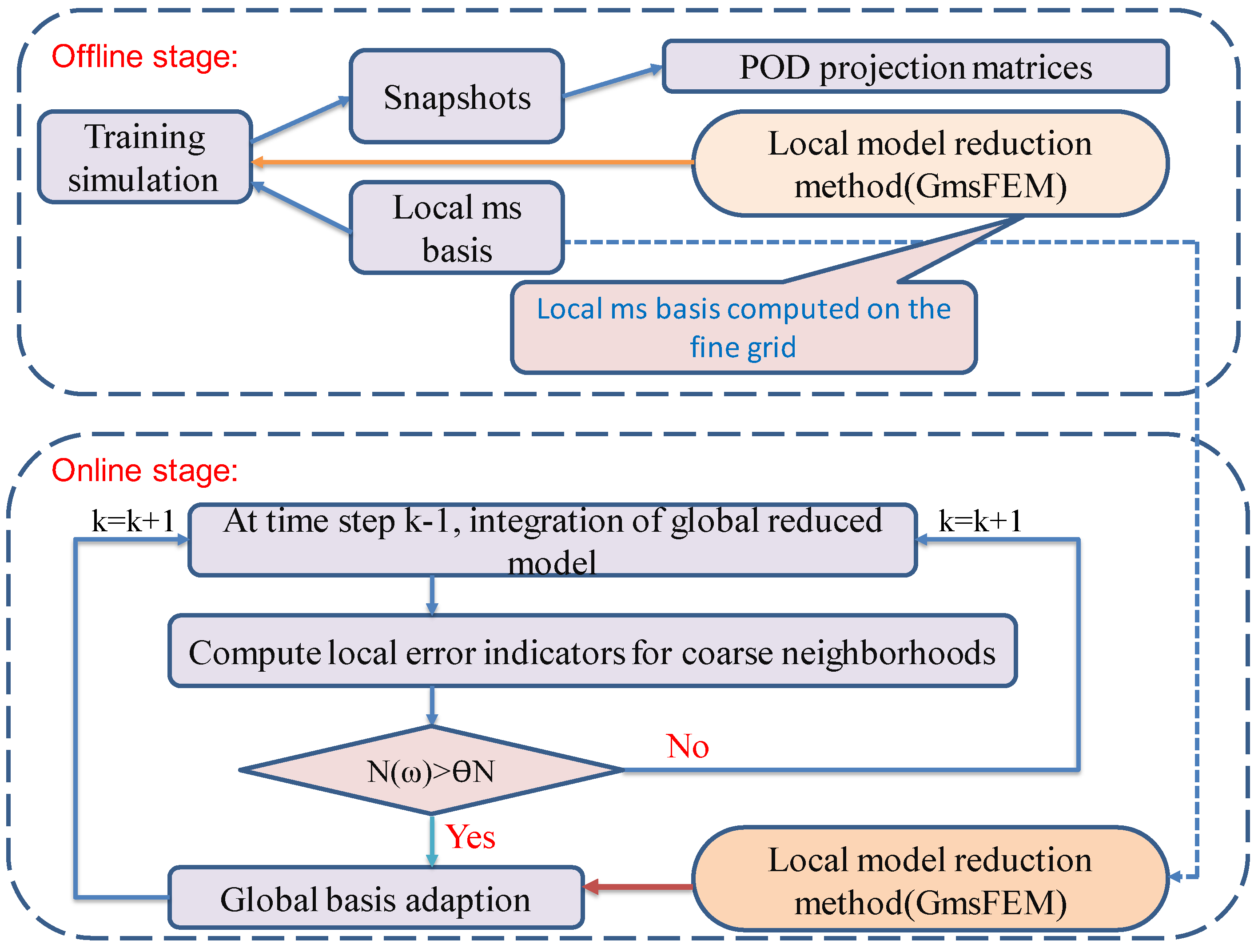
In the linear system setting, one can compute the projection matrices based on the fixed operators offline, that is, outside of the time dependent loop, and perform the reduction by projecting directly onto a much smaller subspace as in Equation (2). However, for nonlinear systems, as in the case of flow in heterogeneous porous media, one cannot perform such projection without having to recompute the operators for every time step. In this case, the best choice is to compute the projection matrices offline and perform the projection and integration of the reduced model online. This setting is particularly useful for the POD-DEIM-based model reduction, whereby the projection matrices are computed offline and are based solely on runs of the fine scale model. In summary, in the offline stage, we construct the reduced order model; in the online stage, given particular parameters or inputs, the reduced model can be approximated efficiently and integrated in time. Online computations have costs that may not depend on the size of the fine scale model. For this reason, we perform the online adaptivity infrequently.

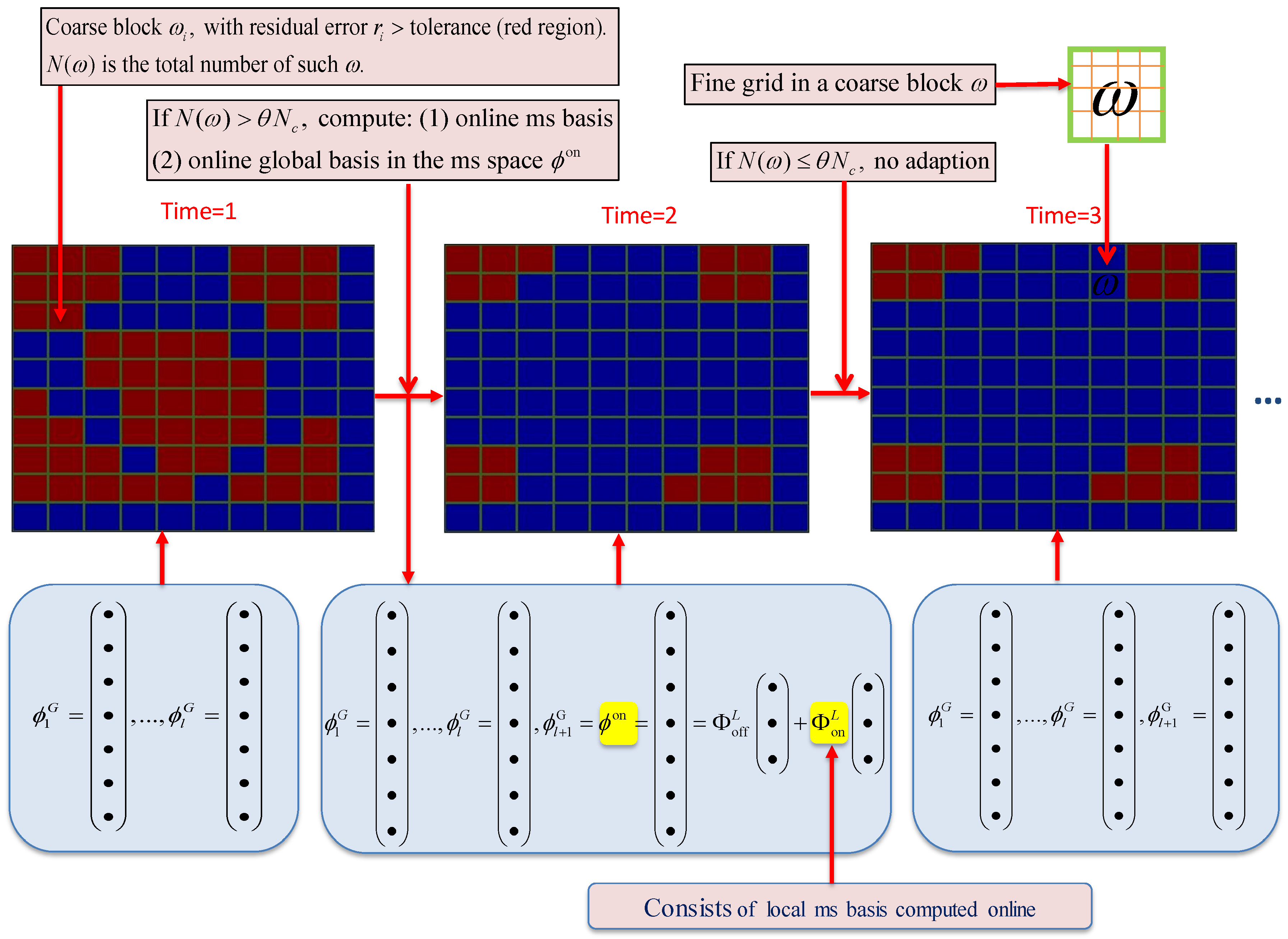
In the online stage, we propose a criterion to decide when updates are required. Once the criterion is satisfied, we adapt the POD subspaces, the DEIM space and the DEIM interpolation points for the nonlinear functions by incorporating new data that becomes available online. For the adaption of the POD subspace, we propose a local-global strategy. First, instead of global error indicators based on the residual which are expensive to compute, we use local error indicators to monitor when global POD basis adaption is needed. By using local error indicators, the computational time can be reduced as one avoids computing global error indicators. Secondly, we employ a local model order reduction method, i.e., the generalized multiscale finite element method (GMsFEM) [17,18,19,20], to solve the global residual problem to get the new POD basis function. Based on local error indicators (see [21,22,23,24] for local error indicators for GMsFEM), some local multiscale basis functions are updated and used to compute the online global modes inexpensively. For the adaption of DEIM, we employ a modified low rank updates method investigated in [25], which introduces computational costs that scale linearly in the number of unknowns of the full-order system. We remark that the offline local-global approaches have been studied in the literature [26,27,28,29]. In the proposed method, we develop online multiscale basis functions for both local and global updates.

Our particular interest here is subsurface flow problems. POD techniques were first used by Vermeulen et al. [30] in the context of subsurface flow problems, e.g., that was a groundwater flow problem with a single water component. Jansen et al. [9,31] applied POD to a two-phase oil-water flow. In [32] TPWL was introduced to solve an oil-water flow system. A local-global multi-scale model reduction was proposed in [33]. A constraint reduction based on POD-TPWL was present in [34]. 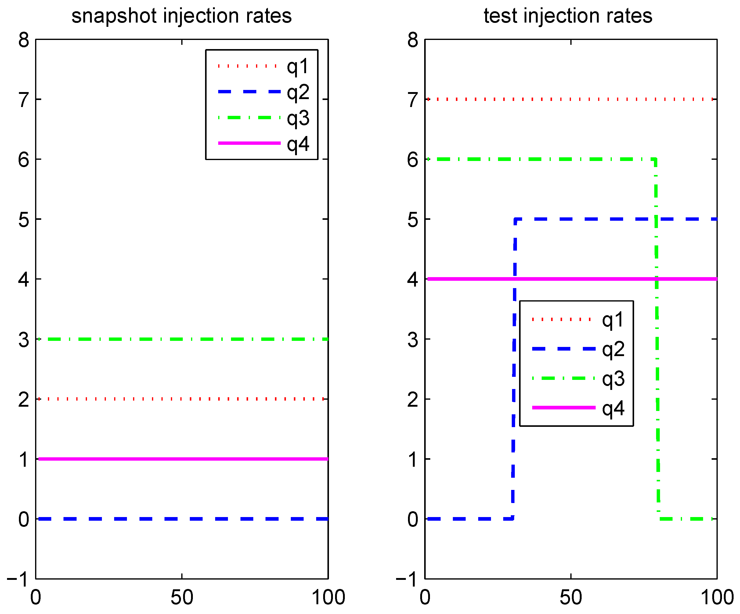In [11,35], POD-DEIM model reduction was used to solve a two-phase flow problem with gravity. 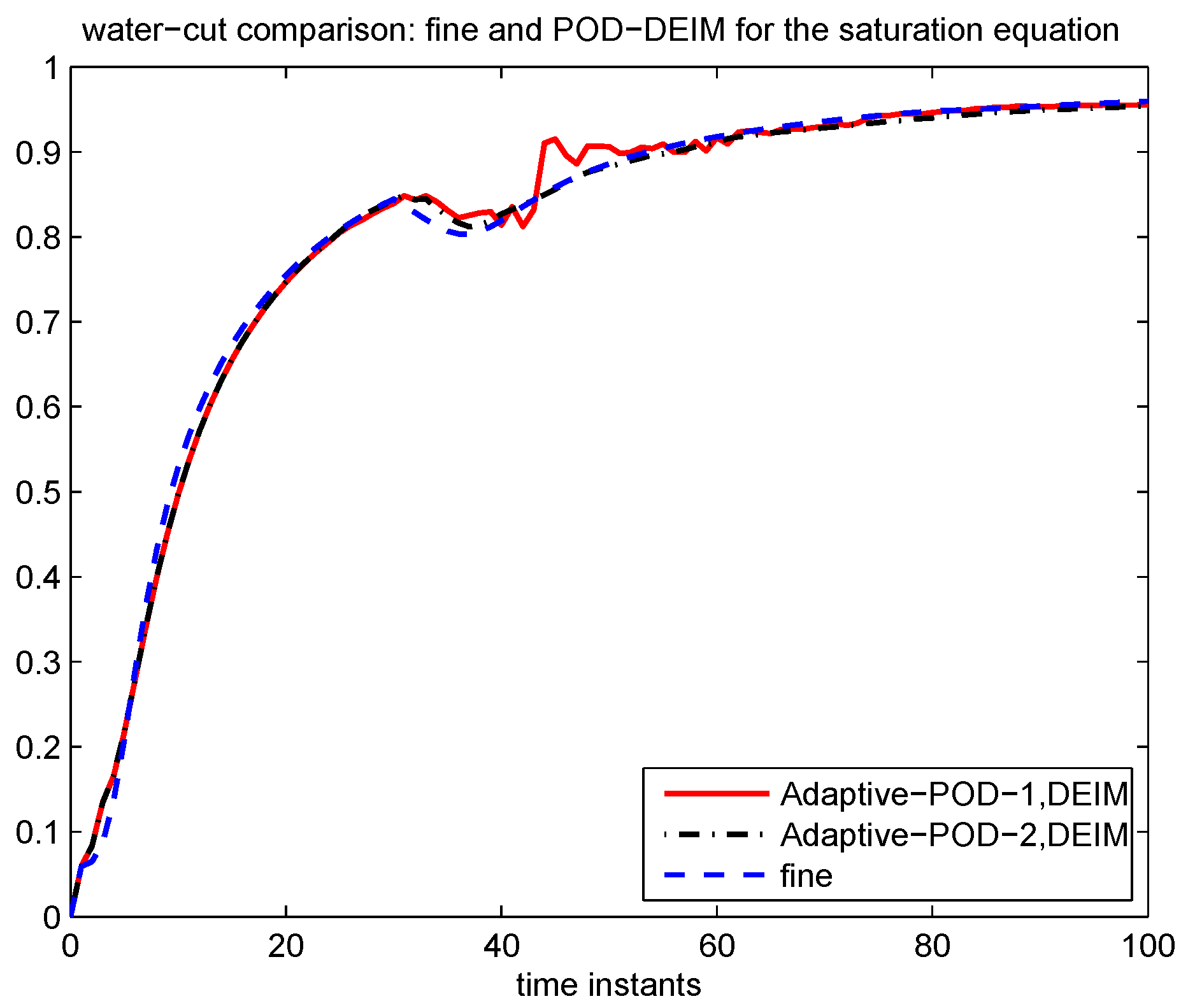However, these methods can only deal with cases that the variation in inputs is within a certain range, i.e., the offline procedure should be able to anticipate almost all the the dynamics of the online system. In many applications, such as optimization and history matching, the final solution trajectory may be hard to predict before the problem is solved. Therefore, a good POD subspace just from using the offline information may not yield robust approximation solutions. Here, we propose to adapt the reduced system by using online data in the online stage. Our numerical results show that one can achieve a good approximation of the solution at a reduced cost.

This paper is organized as follows. In Section 2, the concept of model reduction based on POD-DEIM is given; a short review of POD and DEIM is presented. In Section 3, online adaptive POD is described in Section 3.1, and a discussion of online adaptive DEIM approximation is described in Section 3.2. Applications to single-phase flow and two-phase flow problems are given in Section 4.1 and Section 4.2 respectively. The paper ends with our conclusion in Section 5.

2. Preliminaries

In this section, we will first review the concept of POD-DEIM based model reduction method, which can reduce the dimension of large-scale ODE systems regardless of their origin. A large source of such systems is the semidiscretization of time dependent PDEs. After spatial discretization for a nonlinear PDE, we get a system of nonlinear ODEs of the form

$$\frac{d}{dt}\mathbf{y}(t)=\mathbf{B}\mathbf{y}(t)+\mathbf{f}(\mathbf{y}(t))$$

(1)

where $\mathbf{y}(t)\in {\mathbb{R}}^n,\mathbf{B}\in {\mathbb{R}}^{n\times n}$ is a constant matrix, and $\mathbf{f}(\mathbf{y}(t))$ is a nonlinear function.

We start our exposition by briefly reviewing the global model reduction framework. Let ${\mathbf{V}}_k\in {\mathbb{R}}^{n\times k}(k\ll n)$ be an orthonormal matrix consisting of reduced basis. Replacing $\mathbf{y}(t)$ in Equation (1) by ${\mathbf{V}}_k\tilde{\mathbf{y}}(t)(\tilde{\mathbf{y}}\in {\mathbb{R}}^k)$, and by Galerkin projection of the system (1) onto ${\mathbf{V}}_k$, we get the reduced system of (1) (the super index T means the transpose of a matrix):

$$\frac{d}{dt}\tilde{\mathbf{y}}(t)={\mathbf{V}}_k^T\mathbf{B}{\mathbf{V}}_k\tilde{\mathbf{y}}(t)+{\mathbf{V}}_k^T{\mathbf{f}(\mathbf{V}}_k\tilde{\mathbf{y}}(t)).$$

(2)

The quality of the above POD Galerkin approximation depends on the choice of reduced basis. Snapshot based POD constructs a set of global basis functions from a singular value decomposition (SVD) of snapshots, which are discrete samples of trajectories associated with a particular set of boundary conditions and inputs. It is expected that the samples will be representative of the solution manifold of the problem of interest. Among the various techniques for obtaining a reduced basis, POD constructs a reduced basis that is optimal in the sense that a certain approximation error concerning the snapshots is minimized. The details of POD are presented in Section 2.1.

To evaluate the nonlinear term ${\mathbf{V}}_k^T{\mathbf{f}(\mathbf{V}}_k\tilde{\mathbf{y}}(t))$ in Equation (2), we first need to project the solution from the reduced space to the fine solution space, then evaluate the nonlinear function $\mathbf{f}$ at all the n fine components, finally we project the n fine components back onto ${\mathbf{V}}_k$. The process results in a cost that is as expensive as solving the original system. To handle this inefficiency, we use DEIM [16], which is reviewed in Section 2.2.

The POD-DEIM model reduction method consists of two stages. In the offline stage, given some inputs, which can be boundary conditions, or control parameters, we run several simulations for the system described by Equation (1) to produce snapshots for the solution states (pressure, saturation or concentration in subsurface flow simulation context) and nonlinear functions. POD is performed to construct the reduced subspaces for the states, and interpolants for the nonlinear functions. In the online stage, the approximate solution of the problem is obtained by writing the solution as a linear combination of the reduced basis, which was fixed at the offline phase. Next, we describe in more details the aforementioned process.

2.1. Proper Orthogonal Decomposition

The POD basis in Euclidean space is specified formally in this section. We refer to [36] for more details on the POD basis in general Hilbert space.

Given a set of snapshots $\{{\mathbf{y}}_1,{\mathbf{y}}_2,\cdots ,{\mathbf{y}}_{n_s}\}\in {\mathbb{R}}^n$, let $\mathbb{Y}=\text{span}\{{\mathbf{y}}_1,{\mathbf{y}}_2,\cdots ,$ ${\mathbf{y}}_{n_s}\}$ and $r=\dim (\mathbb{Y})$. A POD basis of dimension $k<r$ is a set of orthonormal vectors ${\{{\mathit{\varphi }}_i\}}_{i=1}^k\in {\mathbb{R}}^n$ whose linear span best approximates the space $\mathbb{Y}$. The basis set ${\{{\mathit{\varphi }}_i\}}_{i=1}^k\in {\mathbb{R}}^n$ solves the minimization problem

$$\underset{{\{{\mathit{\varphi }}_i\}}_{i=1}^k}{min}\sum _j^{n_s}{∥{\mathbf{y}}_j-\sum _{i=1}^k({\mathbf{y}}_j^T{\mathit{\varphi }}_i){\mathit{\varphi }}_i∥}_2^2$$

(3)

with ${\mathit{\varphi }}_i^T{\mathit{\varphi }}_j={\delta }_{ij}$.

It is well known that the solution to Equation (3) is provided by the set of the left singular vectors of the snapshot matrix ${\mathbb{S}}_y=[{\mathbf{y}}_1,{\mathbf{y}}_2,\cdots ,{\mathbf{y}}_{n_s}]\in {\mathbb{R}}^{n\times n_s}$. Applying SVD to ${\mathbb{S}}_y$, we get

$${\mathbb{S}}_y=\mathbf{V}\mathbf{\Lambda }{\mathbf{W}}^T$$

(4)

where $\mathbf{V}=[{\mathbf{v}}_1,\cdots ,{\mathbf{v}}_r]\in {\mathbb{R}}^{n\times r}$, $\mathbf{W}=[{\mathbf{w}}_1,\dots ,{\mathbf{w}}_r]\in {\mathbb{R}}^{n_s\times r}$ are the left and right projection matrices respectively, and $\mathbf{\Lambda }=\text{diag}({\sigma }_1,\cdots ,{\sigma }_r)\in {\mathbb{R}}^{r\times r}$ with ${\sigma }_1\ge {\sigma }_2\ge \cdots {\sigma }_r>0$. The rank of ${\mathbb{S}}_y$ is $r\le \text{min}(n,n_s)$. The first k column vectors ${\{{\mathbf{v}}_i\}}_{i=1}^k$ of $\mathbf{V}$ are selected as the POD basis (the criterion to decide k is explained later ). The minimum $l^2$-norm error from approximating the snapshots using the POD basis is then given by

$$\sum _j^{n_s}{∥{\mathbf{y}}_j-\sum _{i=1}^k({\mathbf{y}}_j^T{\mathbf{v}}_i){\mathbf{v}}_{\mathbf{i}}∥}_2^2=\sum _{i=k+1}^r{\sigma }_i^2.$$

(5)

The appropriate number of POD basis to be retained for a prescribed accuracy can be determined, for example, by means of the fractional energy (see discussions in [37] for selecting modes):

$$E=\frac{\sqrt{{\sum }_{i=1}^k{\sigma }_i^2}}{\sqrt{{\sum }_{i=1}^{n_s}{\sigma }_i^2}}.$$

(6)

A small number of POD basis is retained if the singular values decay fast. This decay depends on the intrinsic dynamics of the system and the selection of the snapshots. In the next section, we review DEIM, which is applied to reduce the nonlinear terms.

2.2. Discrete Empirical Interpolation Method (DEIM)

In the offline stage, we get the snapshots of the nonlinear function $\mathbf{f}(\mathbf{y}(t))$ as:

$$\{\mathbf{f}(\mathbf{y}(t_1)),\cdots ,\mathbf{f}(\mathbf{y}(t_M))\}\in {\mathbb{R}}^n.$$

By applying POD to the above snapshot matrix and selecting the first m eigen-vectors corresponding to the dominant eigen-values, we obtain the DEIM basis $\mathbf{U}\in {\mathbb{R}}^{n\times m}$. DEIM [16] selects m distinct interpolation points $\{p_1,\cdots ,p_m\}\in \{1,\cdots ,n\}$ and assemble the DEIM interpolation points matrix $\mathbf{P}=[e_{p_1},\cdots ,e_{p_m}]\in {\mathbb{R}}^{n\times m},$ where $e_i\in {\{0,1\}}^n$ is the i-th canonical unit vector. The DEIM interpolant of $\mathbf{f}$ is defined by $(\mathbf{U},\mathbf{P})$. The DEIM approximation of $\mathbf{f}$ is derived, based on $(\mathbf{U},\mathbf{P})$, as

$$\mathbf{f}(\mathbf{y}(t))\approx \mathbf{U}{({\mathbf{P}}^T\mathbf{U})}^{-1}{\mathbf{P}}^T\mathbf{f}(\mathbf{y}(t))$$

where ${\mathbf{P}}^T\mathbf{f}(\mathbf{y}(t))$ samples $\mathbf{f}$ at m components only. In what follows, local model reduction will be reviewed.

2.3. Local Model Order Reduction via GMsFEM

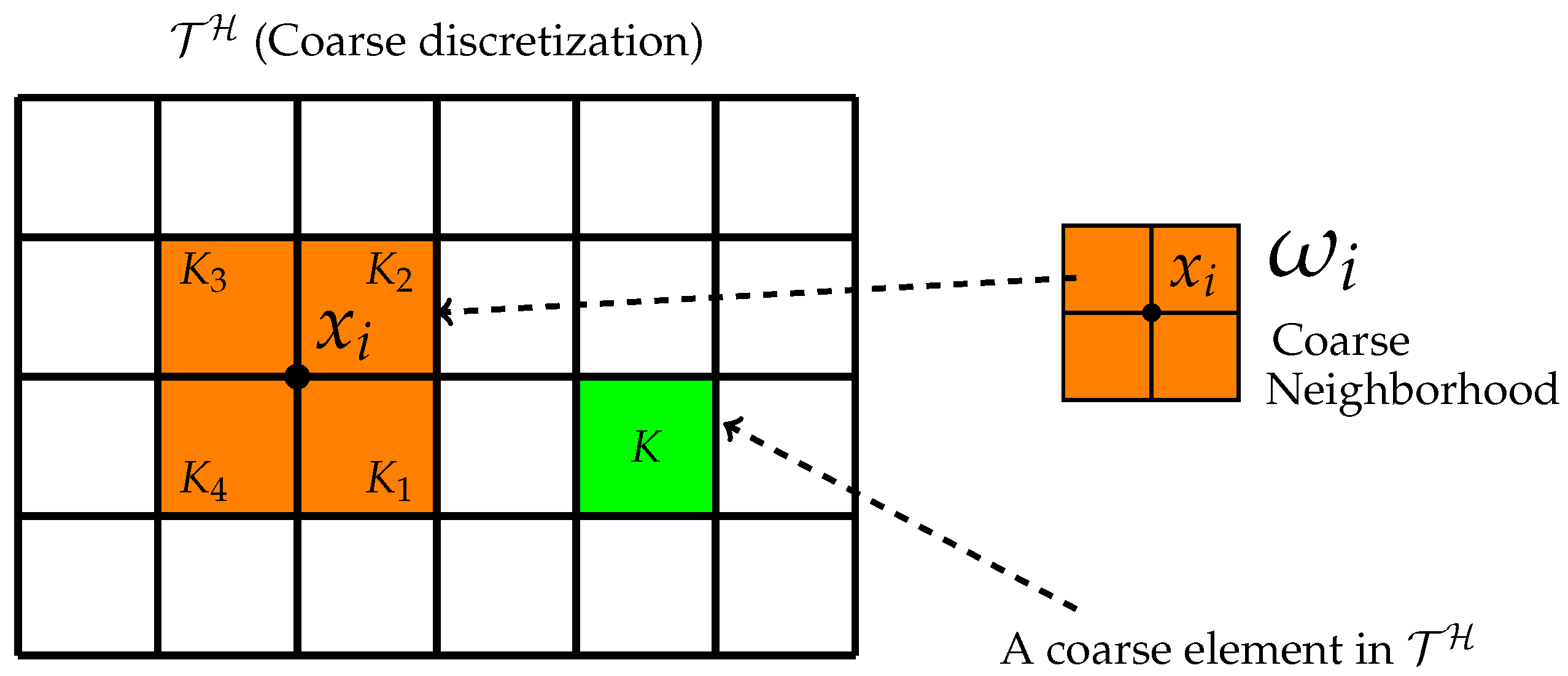
We will give a brief overview of the local model reduction using the GMsFEM [17,18,19,20]. Let ${\mathcal{T}}^{\mathcal{H}}$ be a usual conforming partition of the domain Ω into finite elements called coarse elements, and H is the coarse mesh size. Then, each coarse element is divided into a connected union of fine elements, which are conforming across coarse element faces. 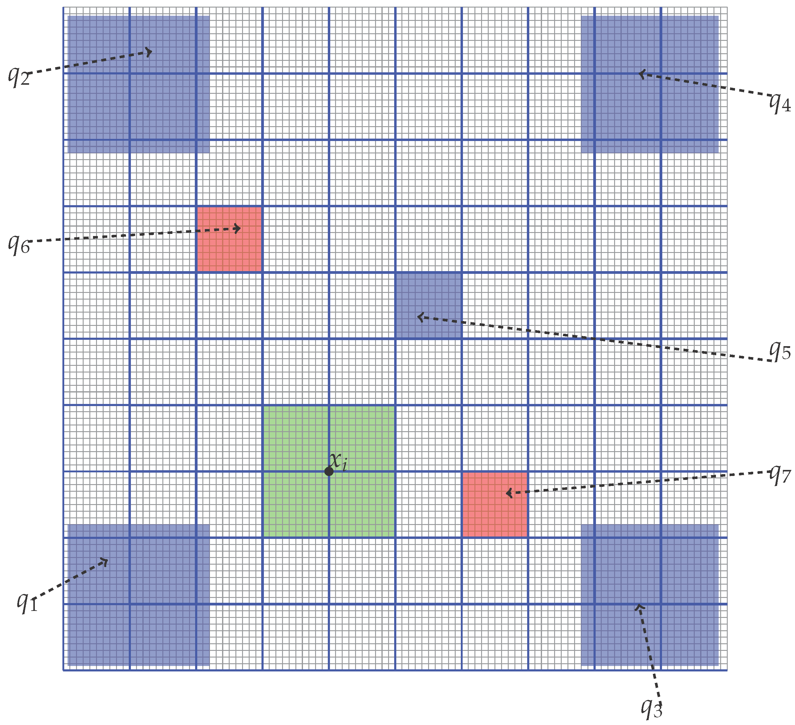This fine grid partition is denoted by ${\mathcal{T}}^h,$ with h as fine mesh size . The fine grid is used to construct the locally supported multiscale basis functions, and compute the reference (fine) solution in the numerical examples. The reference solution is computed on the fine grid. Let $\{x_i|1\le i\le N_c\}$ be the set of nodes on the coarse grid with $N_c$ being the number of nodes in ${\mathcal{T}}^{\mathcal{H}}$. For each coarse node $x_i$, a coarse neighborhood is defined as ${\omega }_i=\bigcup \{K_j\in {\mathcal{T}}^{\mathcal{H}};x_i\in \overline{K_j}\}$. An illustration of the definitions is given in Figure 1. The multiscale basis functions are nodal based and supported on coarse neighborhoods. Specifically, for each coarse node $x_i,$ we construct a set of basis functions $\{{\mathit{\psi }}_k^{{\omega }_i}|k=1,2,\cdots ,L_i\}$ such that each ${\mathit{\psi }}_k^{{\omega }_i}$ is supported on the coarse neighborhood ${\omega }_i$. Note that $L_i$ can be different for different nodes.

Let ω be a given coarse neighborhood, to construct the multiscale basis functions supported on ω, first we construct a snapshot space $V_{\text{snap}}^{\omega }$. $V_{\text{snap}}^{\omega }$ is a set of functions defined on ω and contains all or most necessary information of the fine scale solution restricted to $\omega$. A typical choice of $V_{\text{snap}}^{\omega }$ is local flow solutions, which are constructed by solving local problems with all possible boundary conditions. This can be expensive and for this reason, one can use randomized boundary conditions (see [38,39]) and construct only a few more snapshots than the number of desired local basis functions. Next, we construct the offline space $V_{\text{off}}^{\omega }$ for ω by performing a spectral decomposition of $V_{\text{snap}}^{\omega }$, and choosing the eigenvectors corresponding to the largest eigenvalues. The offline space is defined as ${\Phi }_{\text{off}}^L=\text{span}\{{\mathit{\psi }}_k^i:1\le k\le L_i,1\le i\le N_c\}$. We refer to [17,40] for details. The above computations are performed in the offline stage. For time dependent problems, as time advancing, ${\Phi }_{\text{off}}^L$ may not be good enough to represent the behavior of the full resolved solution at some time instants. We use an adaptive enrichment algorithm which allows one to use more basis functions in regions with large errors. We refer to [40] for details.

3. Online Adaptive POD-DEIM Model Reduction

In this section, we discuss the construction of the online adaptive POD-DEIM model reduction framework. We start with the online adaptive POD and later introduce the adaptive POD-DEIM algorithm.

3.1. Online Adaptive Local-Global Proper Orthogonal Decomposition

We adapt the POD subspaces at some particular instants as time proceeds. Two issues are addressed here: at which instants to adapt, and how to adapt the POD subspaces. The updates are performed online, therefore the goal is to keep the computational cost as low as possible.

The main idea of adaptive local-global POD model order reduction method is summarized in Algorithm 1. The superindex G stands for global, superindex L stands for local, and superindex T means transpose of a matrix. ${\Phi }_{k-1}^G$ is the initial global POD matrix for time step $k-1$. Similarly, ${\Phi }_{k-1}^L$ is the initial local multiscale basis matrix for time step $k-1$. In Figure 2, a flow chat corresponding to Algorithm 1 is given. In Figure 3, we present an schematic description of Adaptive-POD-1. We note that there is no global fine problem computation in the method.

Algorithm 1 Adaptive Local-Global POD Model Order Reduction Method
	OFFLINE STAGE:
1:	Construction of snapshots for states, local off-line space (consists of local ms basis) by GMsFEM
2:	Construction of POD subspaces (POD projection matrices)
	ONLINE STAGE : for step k adaption
3:	INPUT : Global POD basis matrix ${\Phi }_{k-1}^G$, local off-line space ${\Phi }_{k-1}^L$
4:	Solve the reduced system: ${({\Phi }_{k-1}^G)}^T\mathbf{A}{\Phi }_{k-1}^G{\mathbf{X}}_r^{k-1}={({\Phi }_{k-1}^G)}^T{\mathbf{F}}_k$ (Global reduced-order model)
5:	Compute local error indicators, and decide if adaption is needed. If yes, go to 6. Otherwise, go to next time step $k+1$
6:	Solve the global residual problem $\mathbf{A}{\mathit{\varphi }}^{k,\text{online}}={\mathbf{F}}_k-\mathbf{A}{\Phi }_{k-1}^G{\mathbf{X}}_r^{k-1}$ for ${\mathit{\varphi }}^{k,\text{online}}$ by adaptive local method with initial local off-line space ${\Phi }_{k-1}^L$
7:	Update the POD subspace by Adaptive-POD-1 or Adaptive-POD-2
8:	OUTPUT : Global POD basis matrix ${\Phi }_k^G$, local offline space ${\Phi }_k^L$

In the offline stage, a training simulation is run by the GMsFEM. Local multiscale bases are constructed, and snapshots for states at some time steps are saved. Next, POD is performed on the snapshots to construct the POD projection matrices. In the online stage, at every time step we solve a global reduced system, which is usually very small, for example, in Section 4.1, the largest dimension is 8. Next we use our criterion to decide if global basis adaption is necessary. The criterion is specified in the next paragraph. If adaption is needed, a new global basis is obtained by solving a residual problem with GMsFEM. Again, in Section 4.1, a residual problem is of size about ${10}^4$; in

Table 1. Adaptive-POD-1 with 5 initial global POD basis.

Time Instant to Add	$G^{\text{off}}$	$L^{\text{off}}$	$L^{\text{add}}$
1	5	484	119
2	6	484	116
35	7	484	126
Average error	$L^2$	$H^1$
	0.0135	0.0027

, the size of the reduced problem of the residual problem by GMsFEM is about 600.

It is important to monitor when the approximation from the reduced system is no longer sufficiently accurate according to a particular criterion, leading to adaptation of the POD subspaces. This adaption must be performed when the system dynamics has deviated from the current POD subspace as reflected by the residual evaluation. In [41], some residual based POD modes were added to the old POD subspace for Navier-Stokes equations. In [42], a second error estimate based on a second Galerkin system to account for situations in which qualitative changes in the dynamics occur was introduced. In this case, two reduced systems must be solved at a time, thus incurring higher computational cost. In [43], a residual based indicator was used in nonlinear dissipative systems. Here, we propose to use local error indicators based on the multiscale basis, which is cheaper to be computed. The main idea is as follows:

• For coarse blocks ${\omega }_1,{\omega }_2,\cdots ,{\omega }_N$, compute their corresponding $H^{-1}$ norm of the residual, and denote as $r_1,r_2,\cdots ,r_{N_c}$.
• Count the total number $N(\omega )$ of coarse blocks with $r_i>$ a certain error tolerance. Here a large error means the current POD modes cannot give a good representation of the features in that coarse block.
• If $N(\omega )>\theta N_c$, then adaption is needed, θ is a fraction of the total number of coarse blocks.

In general, one can use a threshold for the sum of the local indicators. The choice of the threshold is typically based on experimental results and analysis. The larger the threshold is, more updates are performed. Next, we describe how to update the POD subspace.

For the POD subspace adaption at step k, suppose $N_{k-1}$ number of initial POD modes $\{{\mathit{\varphi }}_1^G,\cdots ,{\mathit{\varphi }}_{N_{k-1}}^G\}$ are given. ${\Phi }^G$ is the POD matrix with $\{{\mathit{\varphi }}_1^G,\cdots ,{\mathit{\varphi }}_{N_{k-1}}^G\}$ as column vectors. We obtain the online snapshot vector ${\mathit{\varphi }}^{k,\text{online}}$ by solving a residual problem (for linear system), or the high fidelity system (for nonlinear system). We illustrate how to get the new online global basis for the linear case. Suppose we are solving Equation (1). At every time step, we need to solve a linear system of the form

$$\mathbf{AX}={\mathbf{F}}_k.$$

(7)

The POD reduced order system for Equation (7) is

$${({\Phi }^G)}^T\mathbf{A}{\Phi }^G{\mathbf{X}}_r={({\Phi }^G)}^T{\mathbf{F}}_k.$$

(8)

The residual is $\mathbf{res}={\mathbf{F}}_k-\mathbf{A}{\Phi }^G{\mathbf{X}}_r$. If update is needed, then we solve the residual problem

$$\mathbf{A}{\mathit{\varphi }}^{k,\text{online}}=\mathbf{\text{res}}$$

(9)

to obtain the online basis ${\mathit{\varphi }}^{k,\text{online}}$.

Note that Equation (9) is expensive to solve because it is a fine-grid problem. We propose to use the local model reduction method as described in Section 2.3 to solve it. In the following, we introduce two methods to adapt the POD subspace after ${\mathit{\varphi }}^{k,\text{online}}$ is obtained. One way is to add ${\mathit{\varphi }}^{k,\text{online}}$ directly to $\{{\mathit{\varphi }}_1^G,\cdots ,{\mathit{\varphi }}_{N_{k-1}}^G\}$, therefore the new POD subspace is the span of $\{{\mathit{\varphi }}_1^G,\cdots ,{\mathit{\varphi }}_{N_{k-1}}^G,{\mathit{\varphi }}^{k,\text{online}}\}$. In this way, the number of POD modes increases by one after every adaption. We denote this method as Adaptive-POD-1.

It is possible that as time proceeds, some modes in the POD subspace become negligible (redundant) in representing the near future dynamics, therefore it can be removed from the POD subspace. This can be achieved in various ways. In our simulations. we follow the following procedure. Apply POD to the set of vectors, see [43]

$$\{w_1{\mathit{\varphi }}_1^G,\cdots ,w_{N_{k-1}}{\mathit{\varphi }}_{N_{k-1}}^G,{\mathit{\varphi }}^{k,\text{online}}\}$$

where the weights $w_i$ are defined as

$$w_i=\text{min}\left\{\frac{{\sigma }_i}{\sqrt{{\sum }_{j=1}^{N_{k-1}}{\sigma }_j^2}},\frac{〈|C_i|〉}{\sqrt{{\sum }_{j=1}^{N_{k-1}}{〈|C_j|〉}^2}}\right\}$$

where ${\sigma }_i$ are singular values associated with ${\mathit{\varphi }}_i,$ $C_i$ is the amplitude of ${\mathit{\varphi }}_i^G,$ i.e., the coefficient of mode ${\mathit{\varphi }}_i^G$, and $〈|C_i|〉$ is the temporal mean value of $|C_i|$ obtained from the reduced system starting from the first instant since the last update until $k-1$. In this way, the weights $w_i$ eliminate those modes whose average energy decreased considerably since the last update. Therefore only a small number of POD modes is retained through the whole simulation. We denote this method as Adaptive-POD-2.

3.2. Online Adaptive DEIM

In this section, we summarize the idea of online adaptive DEIM as in [25]. First, we adapt the DEIM space by rank one updates. Secondly, we adapt the DEIM interpolation points. Its algorithm is given in Algorithm 2. It is shown in [25] that the run time cost of the adaption scales linearly with the number of degrees of freedom of the full-order system.

Algorithm 2 Online Adaptive DEIM [25]

1: INPUT : $({\mathbf{U}}_{k-1},{\mathbf{P}}_{k-1})$, number of sampling points $m_s$, window size w 2: Select $m_s$ points from $\{1,2,\cdots ,n\}$ that are not points in ${\mathbf{P}}_{k-1}$. 3: Assemble sampling points matrix ${\mathbf{S}}_k$ by combining ${\mathbf{P}}_{k-1}$ and the selected points. 4: Compute the coefficient matrix ${\mathbf{C}}_k$ for $[\widehat{\mathbf{y}}(t_k),\widehat{\mathbf{y}}(t_{k-1}),\cdots ,\widehat{\mathbf{y}}(t_{k-w+1})]$ with interpolant $({\mathbf{U}}_{k-1},{\mathbf{S}}_k)$ 5: Solve the minimization problem (10) for ${\mathit{\alpha }}_k,{\mathit{\beta }}_k$ 6: Update basis ${\mathbf{U}}_k={\mathbf{U}}_{k-1}+{\mathit{\alpha }}_k{\mathit{\beta }}_k^T$ 7: Compute $\text{diag}({\mathbf{U}}_k^T{\mathbf{U}}_{k-1})$ 8: Find the index i of the pair of basis vectors which are nearest to orthogonal 9: Let ${\mathbf{u}}_k$ be the $i-\mathrm{th}$ column of the adapted basis ${\mathbf{U}}_k$ 10: Store all other $m-1$ columns of ${\mathbf{U}}_k$ in ${\widehat{\mathbf{U}}}_k\in {\mathbb{R}}^{n\times (m-1)}$ 11: Store all other $m-1$ columns of ${\mathbf{P}}_{k-1}$ in ${\widehat{\mathbf{P}}}_k\in {\mathbb{R}}^{n\times (m-1)}$ 12: Approximate ${\mathbf{u}}_k$ with the DEIM interpolant $({\widehat{\mathbf{U}}}_k,{\widehat{\mathbf{P}}}_k)$ as ${\widehat{\mathbf{u}}}_k={\widehat{\mathbf{U}}}_k{({\widehat{\mathbf{P}}}_k^T{\widehat{\mathbf{U}}}_k)}^{-1}{\widehat{\mathbf{P}}}_k^T{\mathbf{u}}_k$ 13: Find the index $p_k^i$ that corresponds to largest residual of $|{\widehat{\mathbf{u}}}_k-{\mathbf{u}}_k|$ 14: Update interpolation matrix ${\mathbf{P}}_k$: if ${\mathbf{e}}_{p_k^i}$ is not a column of ${\mathbf{P}}_{k-1}$, then for the $i-$ th column of ${\mathbf{P}}_{k-1}$, replace interpolation point ${\mathbf{e}}_{p_{k-1}^i}$ with ${\mathbf{e}}_{p_k^i}$ 15: OUTPUT : $({\mathbf{U}}_k,{\mathbf{P}}_k)$

For the basis adaption for $\mathbf{f}(\mathbf{y}(t))$ at step k, suppose an initial DEIM interpolant $({\mathbf{U}}_{k-1},{\mathbf{P}}_{k-1})$ is given. We extend the interpolation points matrix ${\mathbf{P}}_{k-1}$ as

$${\mathbf{S}}_k=[{\mathbf{e}}_{p_1},\cdots ,{\mathbf{e}}_{p_m},{\mathbf{e}}_{p_{m+1}},\cdots ,{\mathbf{e}}_{p_{m+m_s}}].$$

The extra $m_s$ points are chosen from $\{1,\cdots ,n\}\backslash \{p_1,\cdots ,p_m\}$ randomly. Therefore, we get a new DEIM interpolant $({\mathbf{U}}_{k-1},{\mathbf{S}}_k)$. Note that ${\mathbf{U}}_{k-1}$ is still the same. Next we define a window of size w that contains the vectors of $\widehat{\mathbf{y}}(t_k),\widehat{\mathbf{y}}(t_{k-1}),\cdots ,\widehat{\mathbf{y}}(t_{k-w+1})$ obtained in the previous online computations; an alternative is to also include intermediate states from the Newton-Raphson iterations of the previous online computations. We then construct DEIM approximations of the nonlinear function $\mathbf{f}$ at the vectors $\widehat{\mathbf{y}}(t_k),\widehat{\mathbf{y}}(t_{k-1}),\cdots ,\widehat{\mathbf{y}}(t_{k-w+1})$ with the DEIM interpolant $({\mathbf{U}}_{k-1},{\mathbf{S}}_k)$. For each $\widehat{\mathbf{y}}(t_{k_i})$, the coefficient is derived as

$${\mathbf{c}}_k(\mathbf{y}(t_{k_i}))={({\mathbf{S}}_k^T{\mathbf{U}}_{k-1})}^{+}{\mathbf{S}}_k^T\mathbf{f}(\widehat{\mathbf{y}}(t_{k_i}))$$

which are put as columns in the coefficient matrix ${\mathbf{C}}_k\in {\mathbb{R}}^{m\times w}$. ${({\mathbf{S}}_k^T{\mathbf{U}}_{k-1})}^{+}\in {\mathbb{R}}^{m\times (m+m_s)}$ is the Moore-Penrose pseudo-inverse.

We then derive two vectors ${\mathit{\alpha }}_k\in {\mathbb{R}}^n$ and ${\mathit{\beta }}_k\in {\mathbb{R}}^m$ such that the adapted DEIM basis ${\mathbf{U}}_k={\mathbf{U}}_{k-1}+{\mathit{\alpha }}_k{\mathit{\beta }}_k^T$ minimizes the Frobenius norm of the residual at the sampling points given by ${\mathbf{S}}_k$

$$\parallel {\mathbf{S}}_k^T({\mathbf{U}}_k{\mathbf{C}}_k-{\mathbf{F}}_k){\parallel }_F^2$$

(10)

where ${\mathbf{F}}_k=[\mathbf{f}(\widehat{\mathbf{y}}(t_k)),\cdots ,\mathbf{f}(\widehat{\mathbf{y}}(t_{k-w+1}))]$. The vectors ${\mathit{\alpha }}_k,{\mathit{\beta }}_k$ are obtained by solving a generalized eigenvalue problem, we refer to [25] for details.

Note that the sampling points are only used for the DEIM basis adaptation whereas ultimately the DEIM interpolation points are used for the DEIM approximation.

With the adapted DEIM basis ${\mathbf{U}}_k$ at step k, we also adapt the DEIM interpolation points. The standard DEIM greedy algorithm is computationally expensive to apply in the online stage, since it recomputes all m interpolation points. It is unnecessary to change all interpolation points after a rank-one update to the DEIM basis. Therefore, we adapt the DEIM interpolation points as follows. First, we compute the dot product between the old and the adapted DEIM basis

$$\text{diag}({\mathbf{U}}_k^T{\mathbf{U}}_{k-1}).$$

(11)

If the dot product of two normalized vectors is one, then they are colinear and the adapted basis vector has not been rotated with respect to the previous vector at step $k-1$. If it is zero, they are orthogonal. We select the basis vector ${\mathbf{u}}_k$ of ${\mathbf{U}}_k$ that corresponds to the component of Equation (11) with the lowest absolute value. The new interpolation point $p_k^i$ is derived from ${\mathbf{u}}_k$ following the standard DEIM algorithm. It then replaces the interpolation point $p_{k-1}^i$. Other interpolation points are unchanged.

4. Applications

We present numerical examples to demonstrate the efficiency of the online adaptive POD-DEIM model reduction method. In Section 4.1, we will apply the approach to a time-dependent linear single-phase problem, therefore only adaptive POD is needed. In Section 4.2, we consider a two-phase flow model driven by viscosity. In all examples, we use time step units.

4.1. Single-Phase Flow

In this section, we consider the single-phase flow problem:

$$\begin{array}{ccc}\hfill \frac{\partial \tilde{h}}{\partial t}+\nabla ·a\nabla \tilde{h}& =& q\text{in}\Omega \hfill \end{array}$$

(12)

$$\begin{array}{ccc}\hfill \tilde{h}& =& 0\text{on}\partial \Omega (\text{boundary condition})\hfill \end{array}$$

(13)

$$\begin{array}{ccc}\hfill \tilde{h}(t=0)& =& {\tilde{h}}_0\text{in}\Omega (\text{initial condition}).\hfill \end{array}$$

(14)

Discretizing in a finite element space, for example $Q_1$ which consists of piecewise linear functions on Ω, for space and using backward Euler method for time discretization, we obtain the following algebraic system:

$$(\mathbf{M}+\Delta t\mathbf{S}){\tilde{\mathbf{h}}}^n=\mathbf{M}{\tilde{\mathbf{h}}}^{n-1}+\Delta t{\mathbf{Q}}^n,\text{in}\Omega$$

(15)

where ${\mathbf{M}}_{ij}={\int }_{\Omega }{\psi }_i{\psi }_{j}dx$ is the mass matrix, ${\mathbf{S}}_{ij}={\int }_{\Omega }a\nabla {\psi }_i·\nabla {\psi }_{j}dx$ is the stiffness matrix, ${\psi }_i,{\psi }_j\in {\mathbf{Q}}_1$, $\Delta t$ is the time step size.

In this example, the computational domain is $\Omega ={(0,1)}^2$, a uniform fine mesh with $n=100$ is used. Our proposed approach can also be used for solving problems on unstructured grids. The size of the full-order system at every time step is $10,000$. For the coarse mesh, we use the mesh size $1/10$. The final simulation time is 10, time-stepping size is $\Delta t=0.1$, therefore there are 100 snapshots in total. The logarithm of the permeability field is shown in Figure 4. In the offline stage, the right-side hand function q for the training simulation is only nonzero on the five blue regions in Figure 5. The values of q with respect to time is given in the left figure of Figure 6. In the test simulation, q is given in the right figure of Figure 6, two nonzero regions are added, one is nonzero through 60–80, the other is nonzero through 90–100, which are the red ones in Figure 5. There is a large decrease in the value $q1$ at time instant 35. In

Table 2. Average POD errors.

Number of POD Basis	${\mathit{L}}^{\mathbf{2}}$	${\mathit{H}}^{\mathbf{1}}$
2	0.6114	0.3254
5	0.3470	0.1676
8	0.2956	0.1378
100	0.1830	0.0796

, the average $L^2,H^1$ errors with different number of POD basis are presented. We can see that even if we use all the 100 POD basis, the average $L^2$ error is still about $18\%$. In Table 1, we start with 5 initial global POD basis. The column $G^{\text{off}}$ means the number of initial global POD basis for each time instants, while the column $L^{\text{off}}$ means the number of initial local basis functions, and the column $L^{\text{add}}$ means the number of local basis added to solve the residual problem (9). For instance, for the third row, the first column shows that we need to update at time instant 2; the second column means for time instant 2, the number of initial global POD basis is 6; the third column means for time instant 2, the number of initial local basis functions is 484; the forth column means we add 126 local basis to the multiscale solution space, from which the global basis is obtained. For the whole test simulation, we add basis at time instants 1, 2 and 35, then we get about $1\%$ average $L^2$ error. The relative $L^2,H^1$ errors with respect to time are shown in Figure 7, which show a good agreement of our numerical solution with the reference solution. The reference solution is computed on the fine grid. Here, since the number of POD basis is already very small, we only use the Adaptive-POD-1 method.

4.2. Two-Phase Flow

4.2.1. An Incompressible Two-Phase Flow Model

In this section, we summarize the underlying partial differential equations to simulate porous media flows. In particular, we consider two-phase flow in a reservoir domain (denoted by Ω) under the assumption that the displacement is dominated by viscous effects; i.e., we neglect the effects of gravity, compressibility, and capillary pressure. This assumption is a useful simplification, but the overall methodology can be applied to more general cases. The two phases are water and oil, and they are assumed to be immiscible. We write Darcy’s law for each phase as follows:

$${\mathbf{u}}_l=-\frac{k_{rl}(s_l)}{{\mu }_l}K\nabla \tilde{p}$$

(16)

where ${\mathbf{u}}_l$ is the phase velocity, K is the permeability tensor, $k_{rl}$ is the relative permeability to phase l ($l=o,w$), $s_l$ is saturation, and $\tilde{p}$ is pressure. Throughout the paper, we use a single set of relative permeability.

The mass conservation law for the two phases is:

$$\varphi \frac{\partial s_l}{\partial t}+\nabla ·{\mathbf{u}}_l=q_l.$$

(17)

Combining Darcy’s law, mass conservation, and the property $s_w+s_o=1$, we derive the following coupled system of pressure and saturation equations (we use s instead of $s_w$ for simplicity):

$$\begin{array}{ccc}\hfill \nabla ·\mathbf{u}& =& q_w+q_o\text{in}\Omega \hfill \end{array}$$

(18)

$$\begin{array}{ccc}\hfill \varphi \frac{\partial s}{\partial t}+\nabla ·(f_w(s)\mathbf{u})& =& \frac{q_w}{{\rho }_w}\text{in}\Omega \hfill \end{array}$$

(19)

$$\begin{array}{ccc}\hfill \mathbf{u}·n& =& 0\text{on}\partial \Omega (\text{no flow at boundary})\hfill \end{array}$$

(20)

$$\begin{array}{ccc}\hfill s(t=0)& =& s_0\text{in}\Omega (\text{initial known saturation})\hfill \end{array}$$

(21)

where ϕ is the porosity, λ is the total mobility defined as

$$\lambda (s)={\lambda }_w(s)+{\lambda }_o(s)=\frac{k_{rw}(s)}{{\mu }_w}+\frac{k_{ro}(s)}{{\mu }_o}$$

(22)

$f_w(s)$ is the flux function,

$$f_w(s)=\frac{{\lambda }_w(s)}{\lambda (s)}=\frac{k_{rw}(s)}{k_{rw}(s)+\frac{{\mu }_w}{{\mu }_o}{k}_{ro}(s)}$$

(23)

and $\mathbf{u}={\mathbf{u}}_w+{\mathbf{u}}_o=-\lambda (s)K\nabla \tilde{p}$ is the total flux. Moreover, $q_w$ and $q_o$ are volumetric source terms for water and oil.

Here, we follow the sequential formulation, that is at each time step one solves for pressure first and then uses the result to solve for the saturation. The pressure equation is solved by mixed finite element method, see [35,44] which produces mass conservative velocity field, and the saturation equation is solved by finite volume method.

4.2.2. Numerical Example

We apply the online adaptive model reduction method to an oil-water flow model with the structure of a 5-spot. A 5-spot pattern is a well configuration that involves 1 producing well (or 1 injector well) in the center and 4 injecting wells (or 4 producers) in the corners of a Cartesian grid. It can be seen as a five wells (point source) in the whole domain. It is designed to maximize the reservoir sweep as water is being injected into the reservoir. Here we set four injection wells in the corners and one production well in the middle of the domain. All the wells are rate controlled. The computational domain is $\Omega ={(0,1)}^2$, a uniform fine mesh with $h=1/220$ is used. The fluid viscosity ratio is ${\mu }_w/{\mu }_o=0.2$. To get the snapshots, we simulate the flow with end of simulation time 800, time stepping size $\Delta t=4$, with well rates as shown in the left in Figure 8. From this forward (training) simulation, we save the snapshots of the states and the nonlinear functions at every 2 units in time. Therefore, 100 snapshots are saved for the states and nonlinear functions. Each snapshot is reshaped to a column vector and is stacked in a snapshot matrix. After applying POD to each matrix, we get the POD subspace. For the test simulation, total simulation time is $400,\Delta t=4$, and the well rates are given in the right of Figure 8.

From Figure 8 we see that the rates are constant for the training simulation, and well 2 is shut off all the time; while for the test simulation, well 2 is open at the time instant 31 and well 3 is closed from 80 to the end of simulation time. Large deviations in the rates of the training and test simulation start at three points: the beginning since different constants are used for rates; time instant 31; time instant 80. These deviations are expected to result in requirement of online adaption. We use the $L^2$ norm of the residual as indicators for adaption. To better understand the impact of injection rates on the whole system, we will investigate the method for the pressure and saturation equations separately first. For the adaptive DEIM application, number of sampling points is $m_s=800$, and window size is $w=25$.

In Case 1, we apply POD reduction to the pressure equation only, while solve the saturation equation on the fine grid. Note that only POD reduction is used, no DEIM is involved since the pressure equation is linearly dependent on the pressure and velocity. The selection criterion (6) for choosing the number of initial POD basis is to capture 99.99% of the energy of the snapshots. In Figure 9, relative saturation errors for 3 scenarios with 5 initial POD basis for flux are given. The red line is for static POD without updating, the errors are greater than 10% all the time, and there are jumps at time instants {31,80}. The blue line is for adaptive POD with adaption at time instants {1,31}. The dot purple line is for adaptive POD with adaption at time instants {1,31,80}, which gives a good accuracy. Figure 10 presents the comparison of water-cut (water flux fractional function $f_w(s)$) corresponding to these 3 scenarios with the fine water-cut. Both figures show that adaption is necessary in order to obtain a good accuracy.

In Case 2, we apply model reduction to the saturation equation only while solving the pressure equation on the fine grid. First, we consider POD without DEIM. As pointed out in Section 2, due to the nonlinearity of the saturation equation, no improvement in efficiency will be achieved if no DEIM is used. We only consider this case to compare with the case for POD-DEIM in the next example. We will see that the POD-DEIM needs more updates than POD. The selection criterion (6) for choosing the number of initial saturation POD basis is to capture 99% of the energy of the snapshots. 20 initial saturation POD basis is selected. Updates are needed at $\{1,4,31,32,33,35,36,38,40,42,43\}$. In

Table 3. Number of POD basis for saturation after each update of POD subspace for Equation (19).

	1	4	31	32	33	35	36	38	40	42	43
Adaptive-POD-1	21	22	23	24	25	26	27	28	29	30	31
Adaptive-POD-2	22	16	8	8	7	7	7	7	7	7	7

, the numbers of saturation POD basis after updating for Adaptive-POD-1, Adaptive-POD-2 are presented. For example, the number of basis for Adaptive-POD-1 after updating at time instant 33 is 25, the number of basis for Adaptive-POD-2 after 4 is 16. The relative saturation errors for both Adaptive-POD-1 and Adaptive-POD-2 are given in Figure 11, we can see that Adaptive-POD-2 delivers almost the same accuracy while using much less number of basis compared with Adaptive-POD-1. The comparison of water-cut between the solutions of Adaptive-POD-1, Adaptive-POD-2 and the fine solution is shown in Figure 12, which shows a good agreement. Second, we apply POD-DEIM to the saturation equation. We use the adaptive DEIM technique as described in Section 3.2 to approximate $f_w$. 15 initial DEIM basis functions are selected for $f_w$. The comparison of water-cut between the solution of Adaptive-POD-2-DEIM, Adaptive-POD-2-DEIM and the fine solution is shown in Figure 13, they are in good agreement in general. The saturation errors for both Adaptive-POD-1-DEIM and Adaptive-POD-2-DEIM are given in Figure 14. We can see that the error of Adaptive-POD-2-DEIM is less than Adaptive-POD-1-DEIM, while the number of basis for Adaptive-POD-2 is less than Adaptive-POD-1.

In Case 3, apply our model reduction method to the coupled system, i.e., POD for the pressure equation and POD-DEIM for the saturation equation. Velocity needs updates at $\{1,31,36,48,80\}$, and saturation needs 13 updates at instants as listed in the

Table 4. Number of POD basis for saturation after each update of POD subspace for the coupled system.

	1	4	31	32	34	35	36	38	39	47	53	54	60
Adaptive-POD-1	21	22	23	24	25	26	27	28	29	30	31	32	33
Adaptive-POD-2	21	16	8	8	7	7	7	7	7	7	7	7	7

. The numbers of saturation POD basis after updating for Adaptive-POD-1, Adaptive-POD-2 are shown in Table 4. The saturation error is given in Figure 15, from there we see that Adaptive-POD-2 has better performance than Adaptive-POD-1. The comparison of water-cut between the solution of Adaptive-POD-1, Adaptive-POD-2 and the fine solution is shown in Figure 16. We observe good agreement.

5. Conclusion

We presented an online adaptive local-global POD-DEIM model reduction method for nonlinear systems where both POD subspaces and DEIM interpolants are adapted during the online stage by incorporating online information locally. In the global adaptive framework, we employ local techniques to realize adaption leading to computational savings in evaluating the residual. Our approach is particularly useful for situations where it is desired to solve the reduced system for inputs or controls that result in a solution outside the span of the snapshots generated in the offline stage. This happens in many applications, such as inverse problem and optimization, where the final solution path may be difficult to predict before the problem is solved. Our method also offers an alternative to constructing a robust reduced system even if a potential initial poor choice of snapshots is used, since it can absorb representative information into the POD solution space along the online simulation process. Future work includes finding an efficient way to obtain the online basis for a nonlinear system.