
Applicability of URANS and DES Simulations of Flow Past Rectangular Cylinders and Bridge Sections

Abstract
:1. Introduction
2. Numerical Approaches
2.1. Solver
2.2. Turbulence Modeling
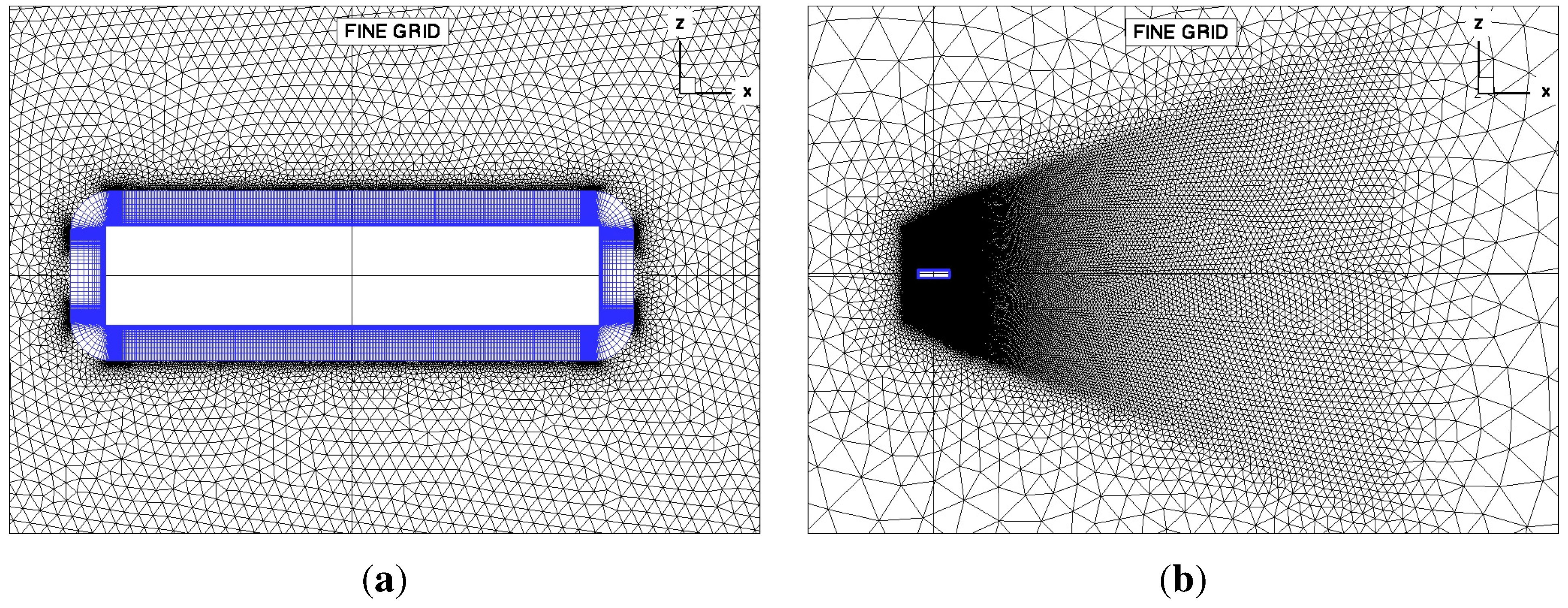
2.3. Spatial and Temporal Discretization
2.4. Boundary and Initial Conditions
3. Rectangular Cylinders
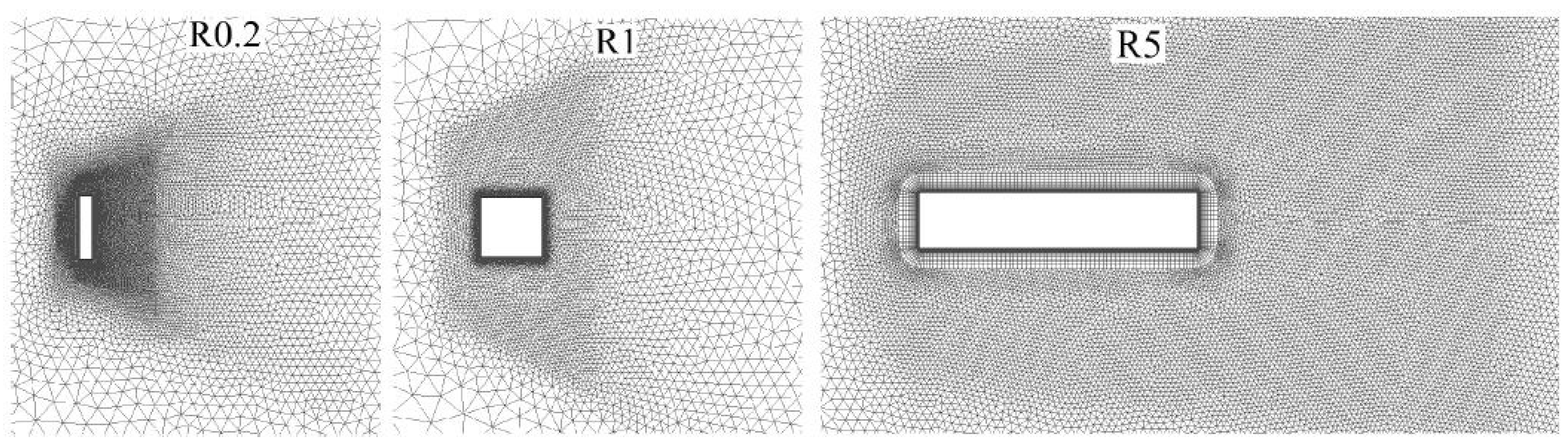
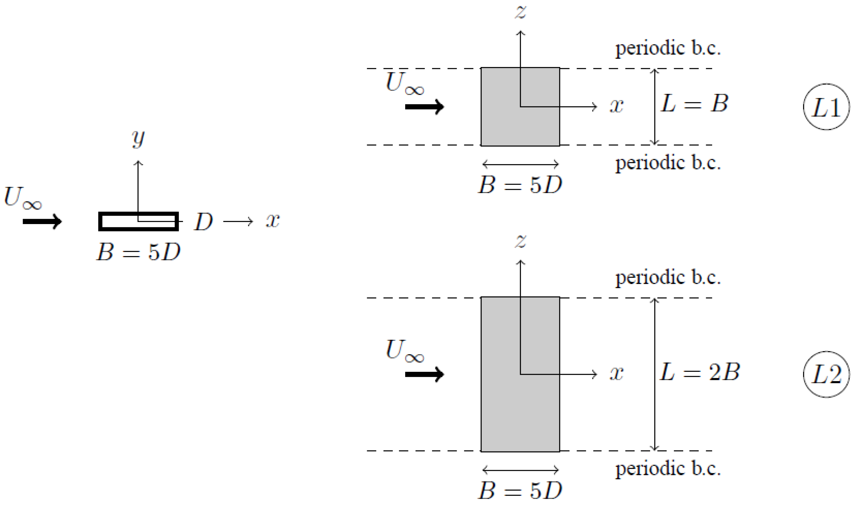
3.1. Effect of the Side Ratio


| = 0.2 | = 1 | = 5 | |||||
|---|---|---|---|---|---|---|---|
| 2D URANS | 3D URANS | Exp. [30,31] | 2D URANS | Exp. [32,33,34] | 2D URANS | Exp. [35,36,37] | |
| 3.06 | 2.0 | 1.9 to 2.0 | 1.91 | 1.9 to 2.3 | 1.06 | 1.03 | |
| 0.49 | 0.08 | 0.2 | 0.28 | 0.08 to 0.23 | 0.02 | ||
| 0.59 | 0.05 | 1.14 | 1.05 | 0.5 | |||
| 0.12 | 0.14 | 0.13 | 0.12 | 0.13 | 0.09 | 0.11 to 0.13 | |
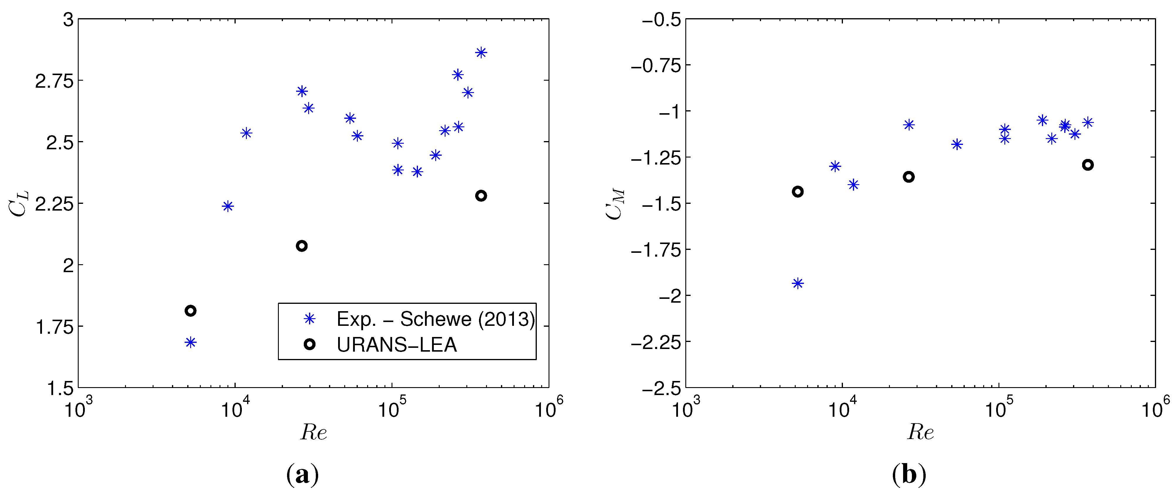
3.2. Reynolds Number Effects


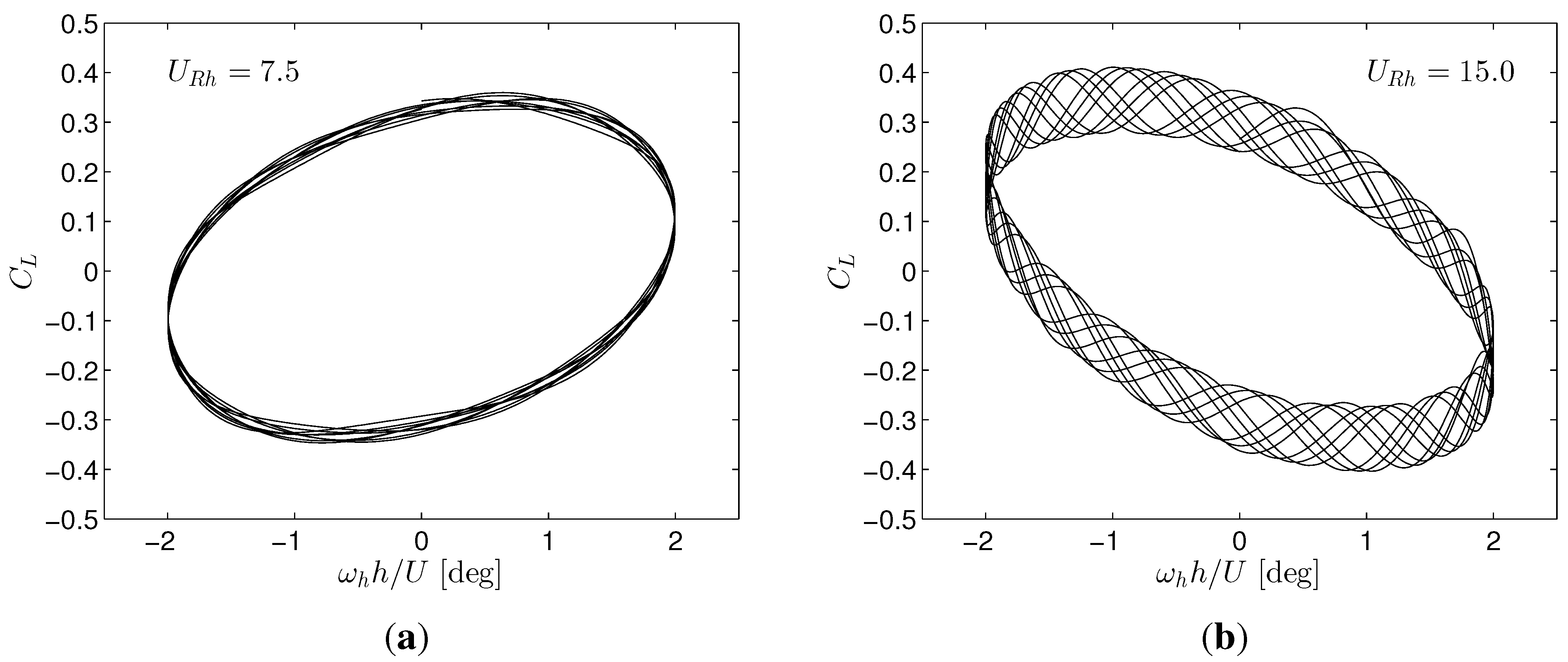
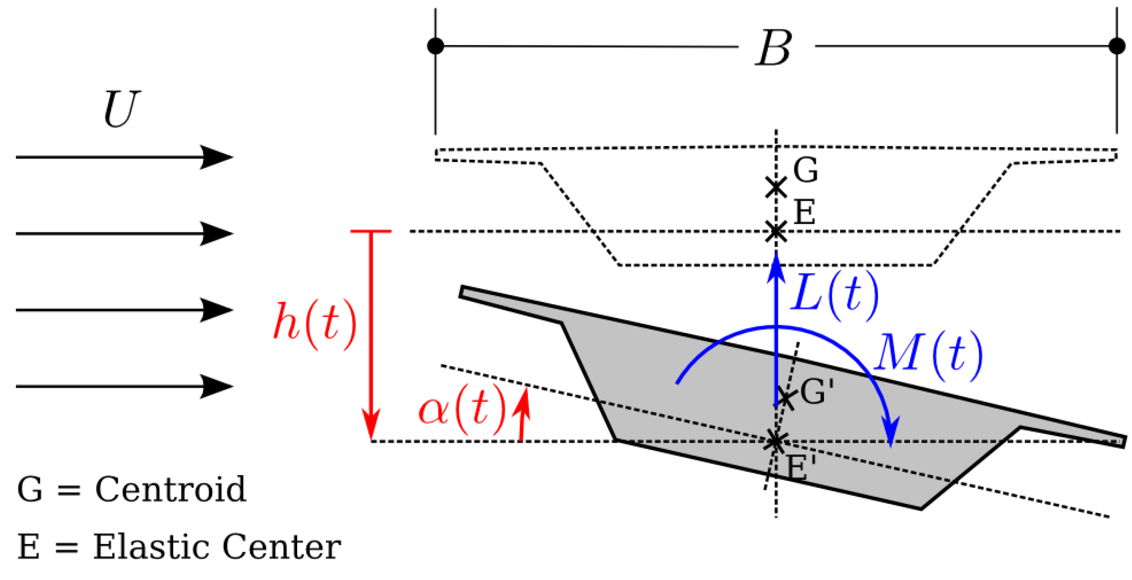
3.3. Forced Vibration Analysis


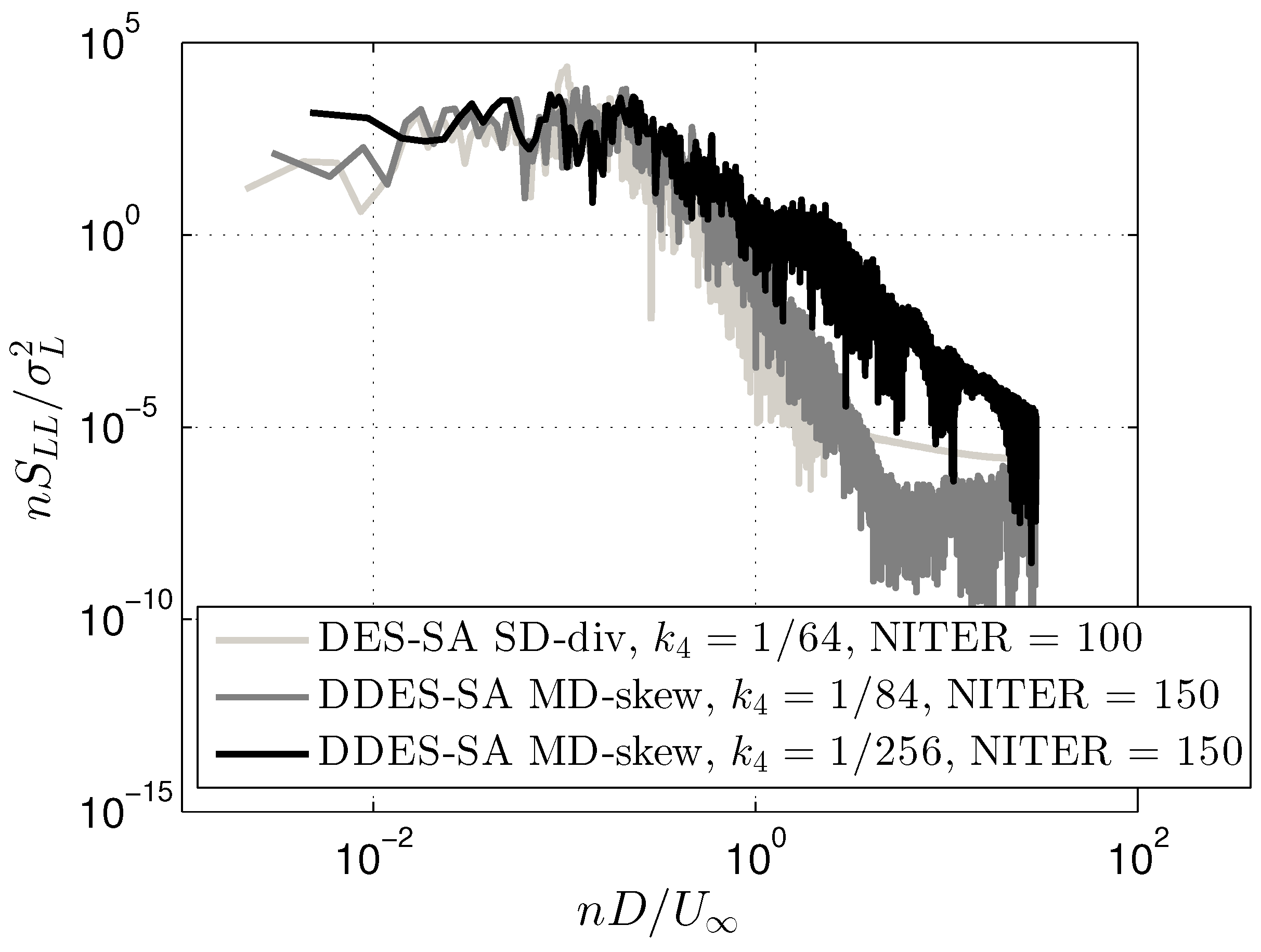
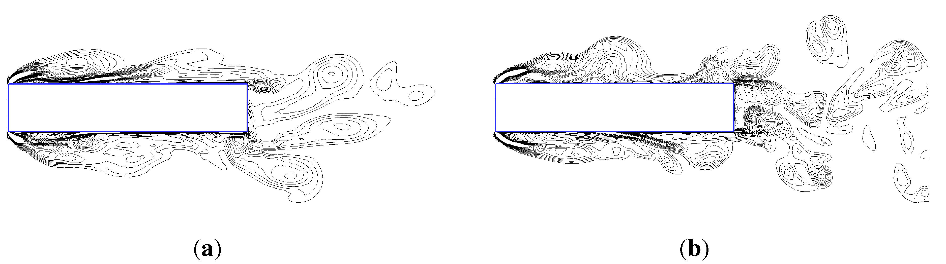
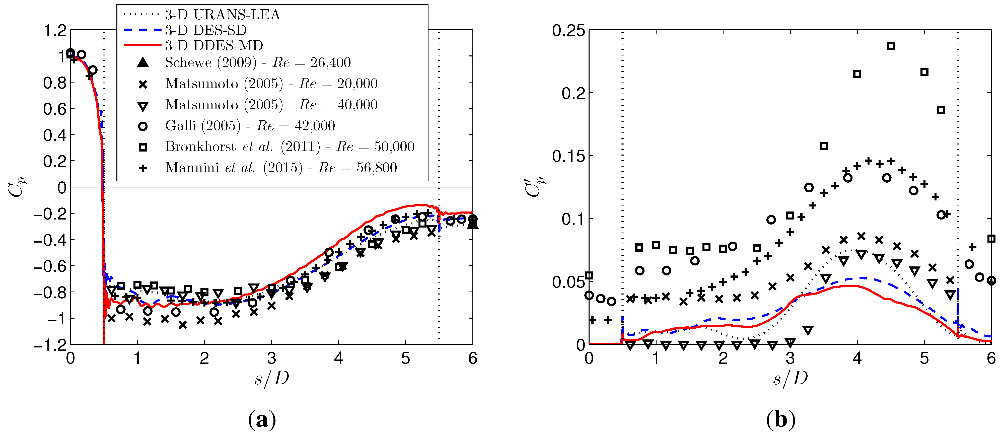
3.4. Three-Dimensional DES Simulations

| NITER | |||||||||
|---|---|---|---|---|---|---|---|---|---|
| URANS-LEA SD-div | 1.0 | - | 1/64 | 100 | 0.095 | 1.071 | 1.035 | 0.029 | 84.5 |
| DES-SA SD-div | 1.0 | 0.45 | 1/64 | 100 | 0.103 | 1.016 | 0.553 | 0.055 | 464.5 |
| DES-SA SD-div | 2.0 | 0.45 | 1/64 | 100 | 0.102 | 1.029 | 0.421 | 0.043 | 715.0 |
| DDES-SA MD-div | 1.0 | 0.65 | 1/84 | 100 | 0.118 | 0.971 | 0.356 | 0.042 | 227.9 |
| DDES-SA MD-div | 1.0 | 0.65 | 1/84 | 150 | 0.119 | 0.967 | 0.333 | 0.035 | 225.6 |
| DDES-SA MD-skew | 1.0 | 0.65 | 1/84 | 150 | 0.114 | 0.965 | 0.343 | 0.037 | 308.3 |
| DDES-SA MD-skew | 1.0 | 0.65 | 1/256 | 150 | 0.087 | 0.998 | 0.173 | 0.030 | 213.3 |
| Experiments [37] | 10.9 | 0.111 | 1.029 | ∼0.4 |


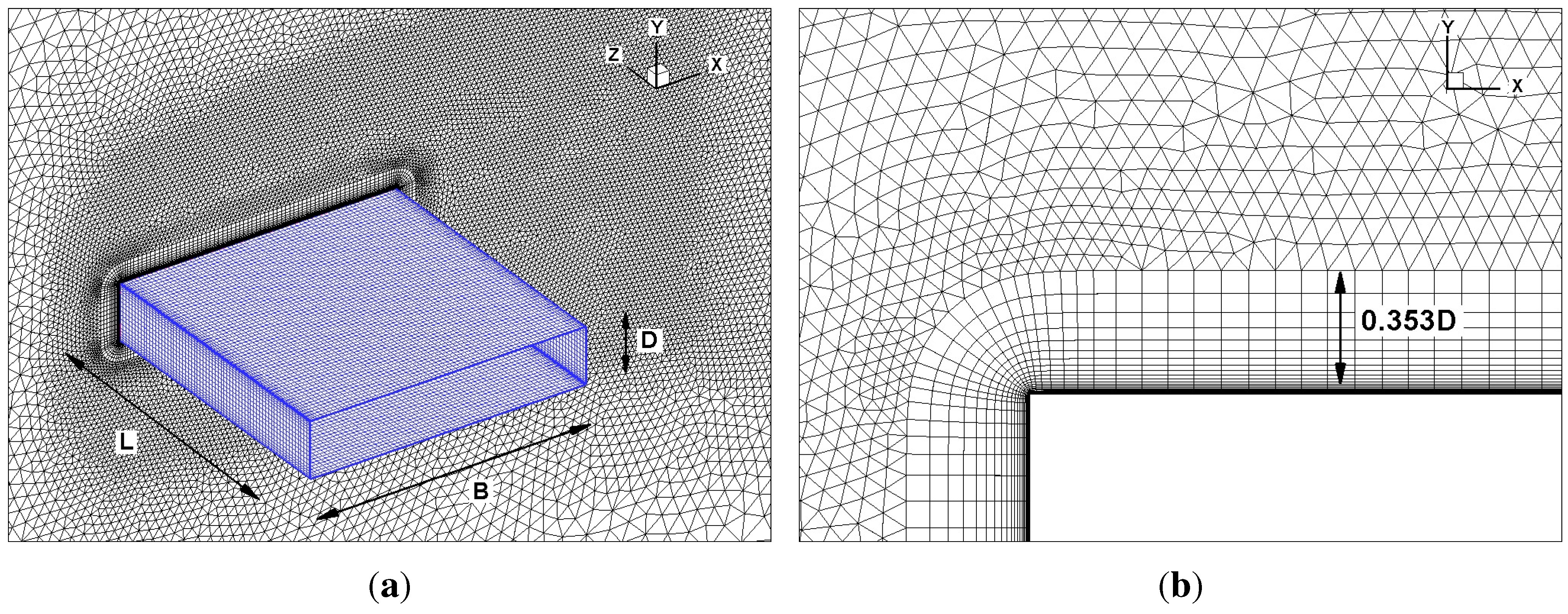
4. Bridge Section
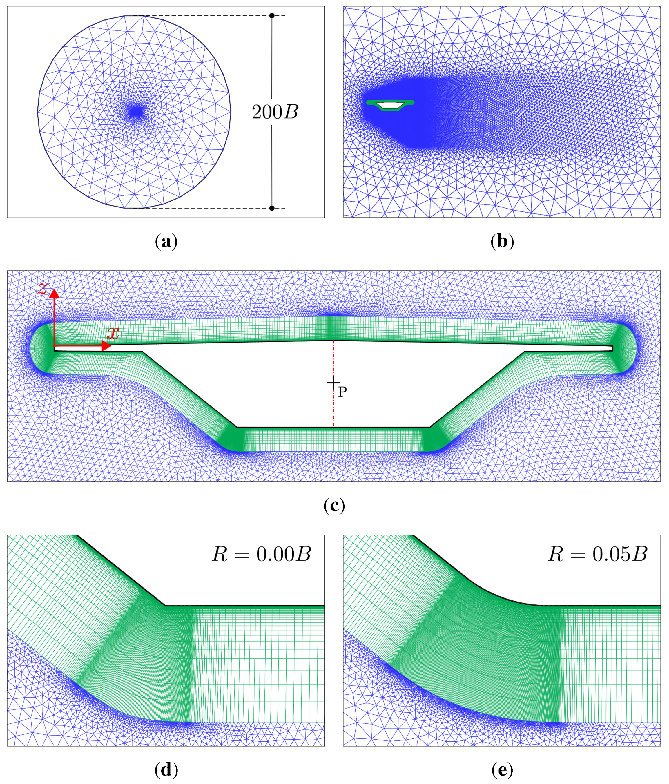
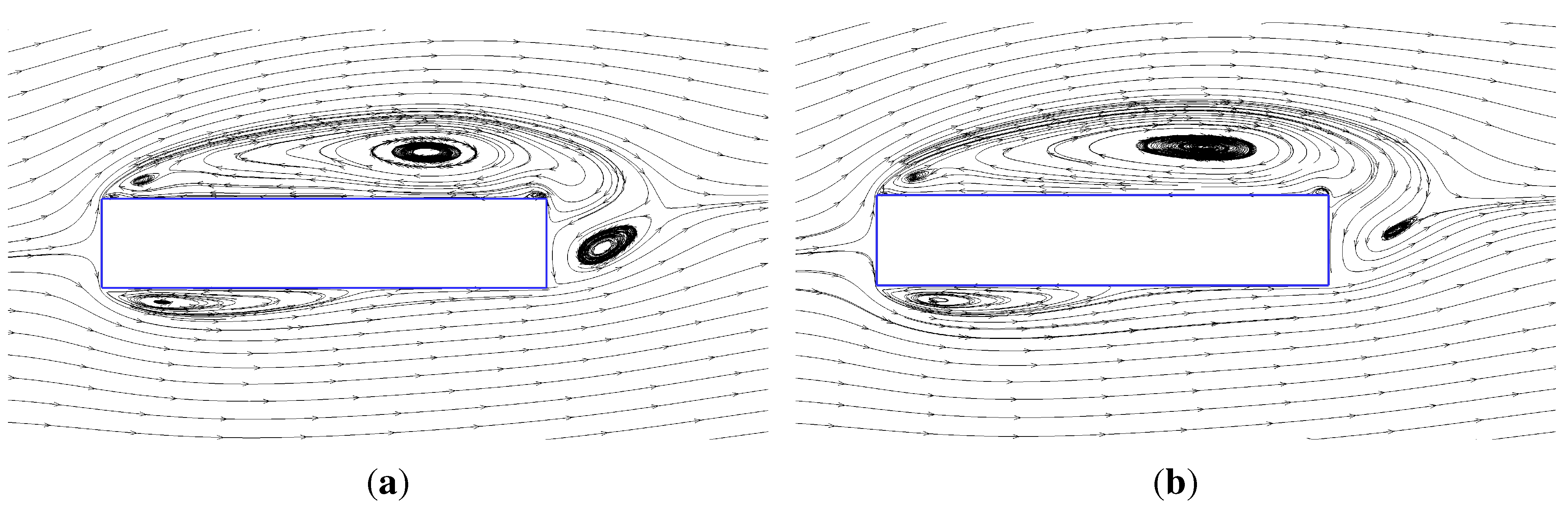
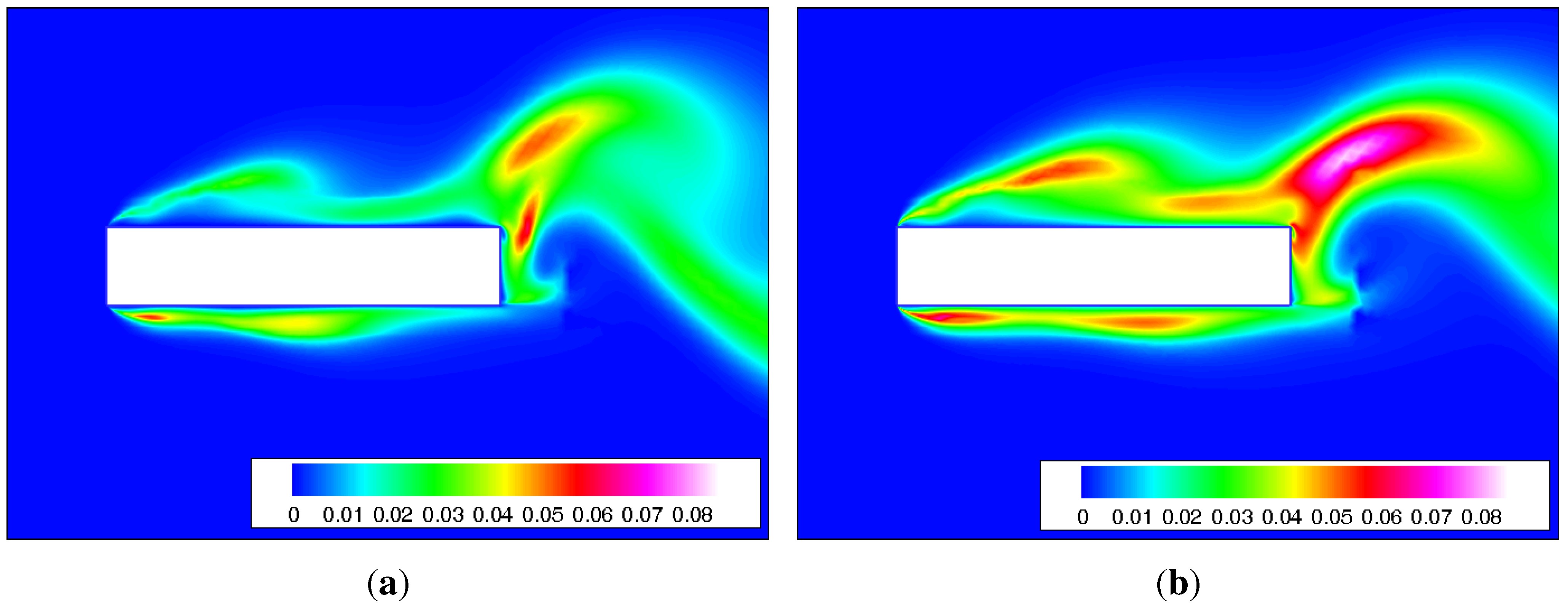
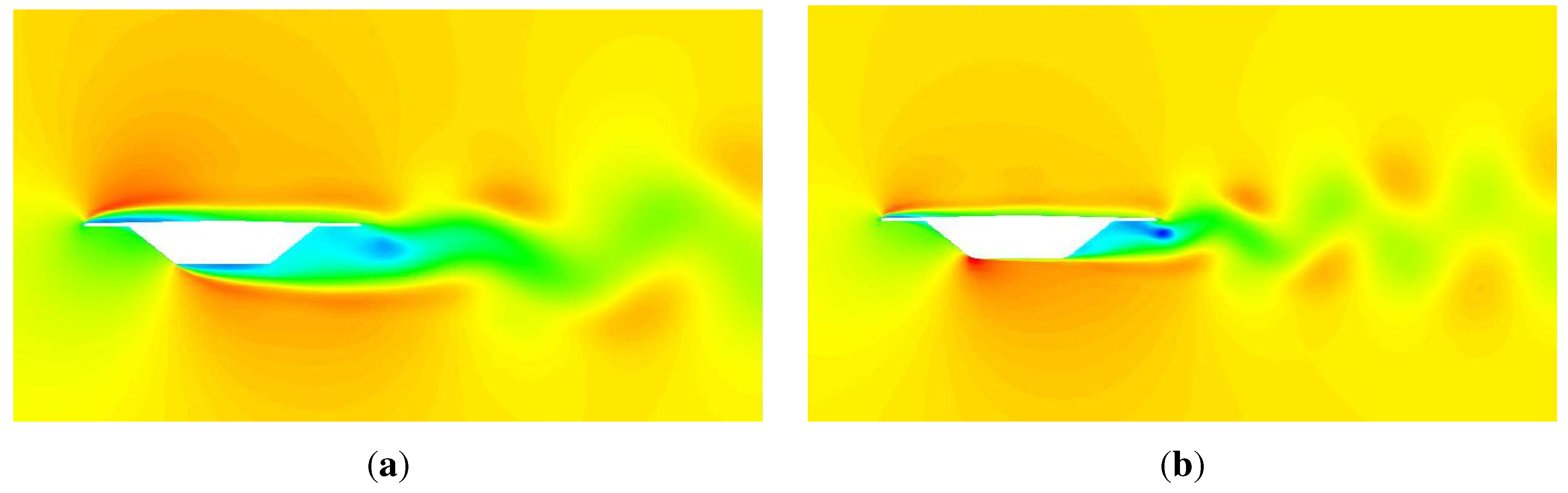
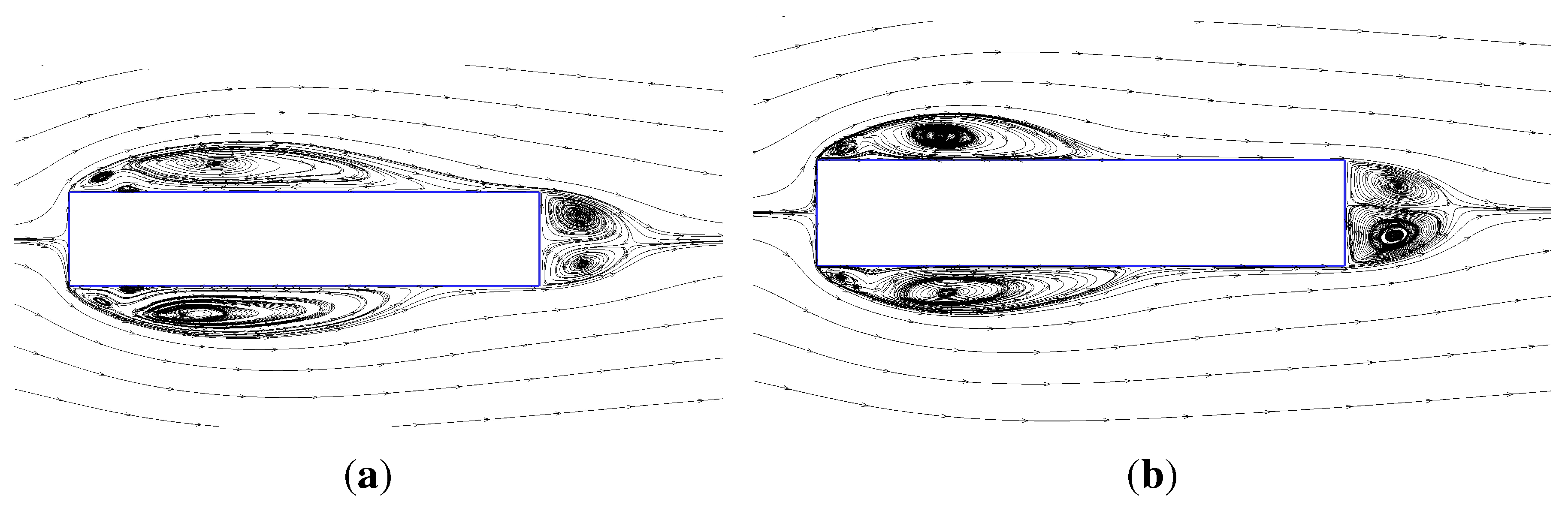
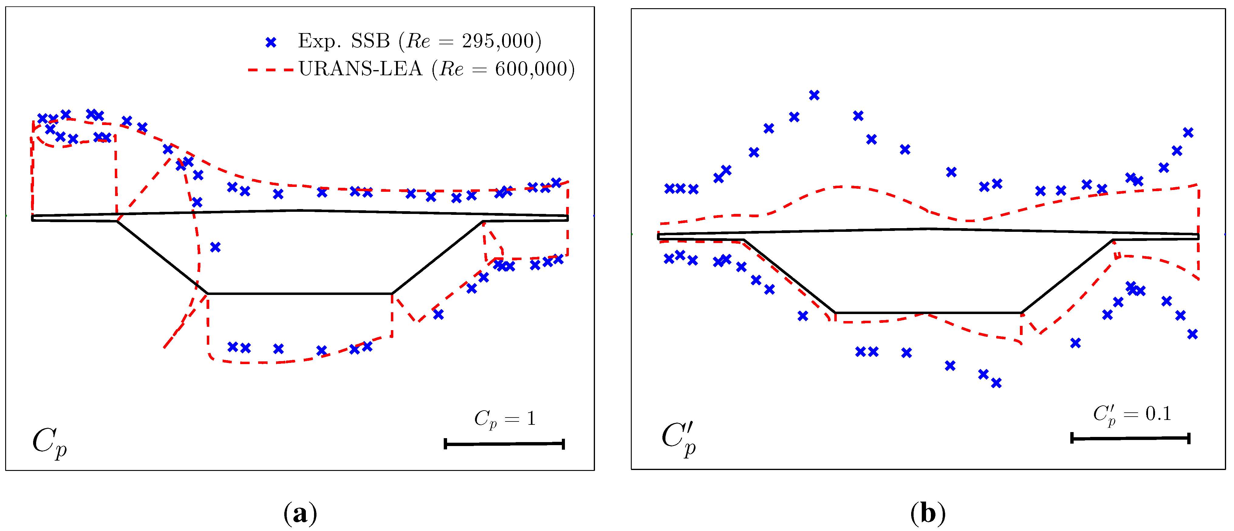
4.1. Stationary Case


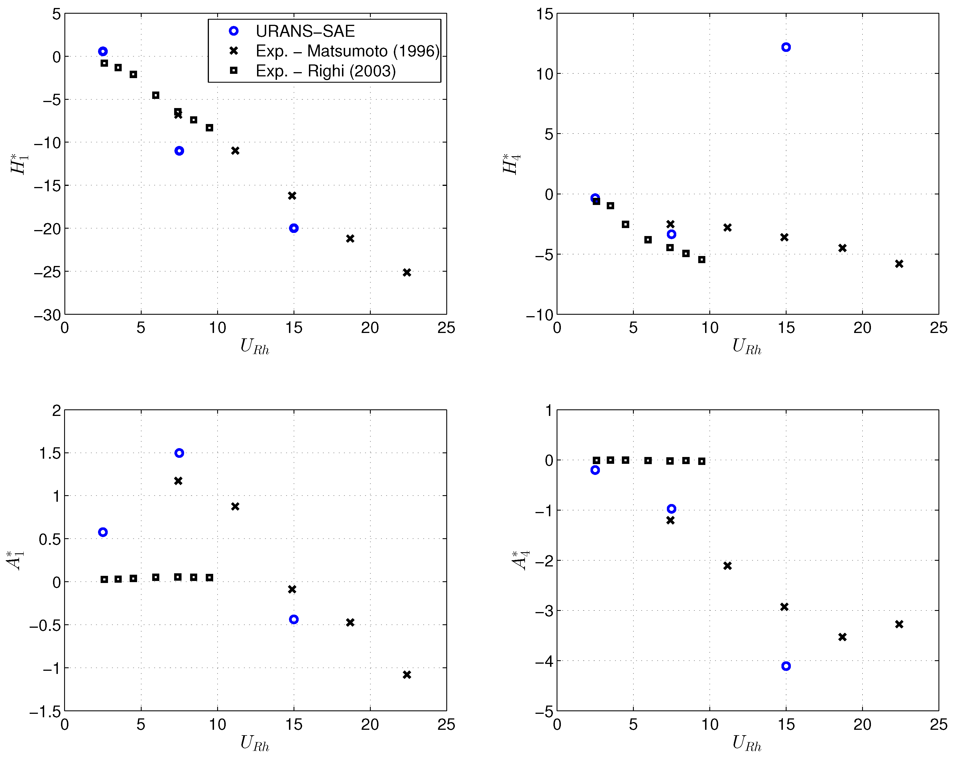
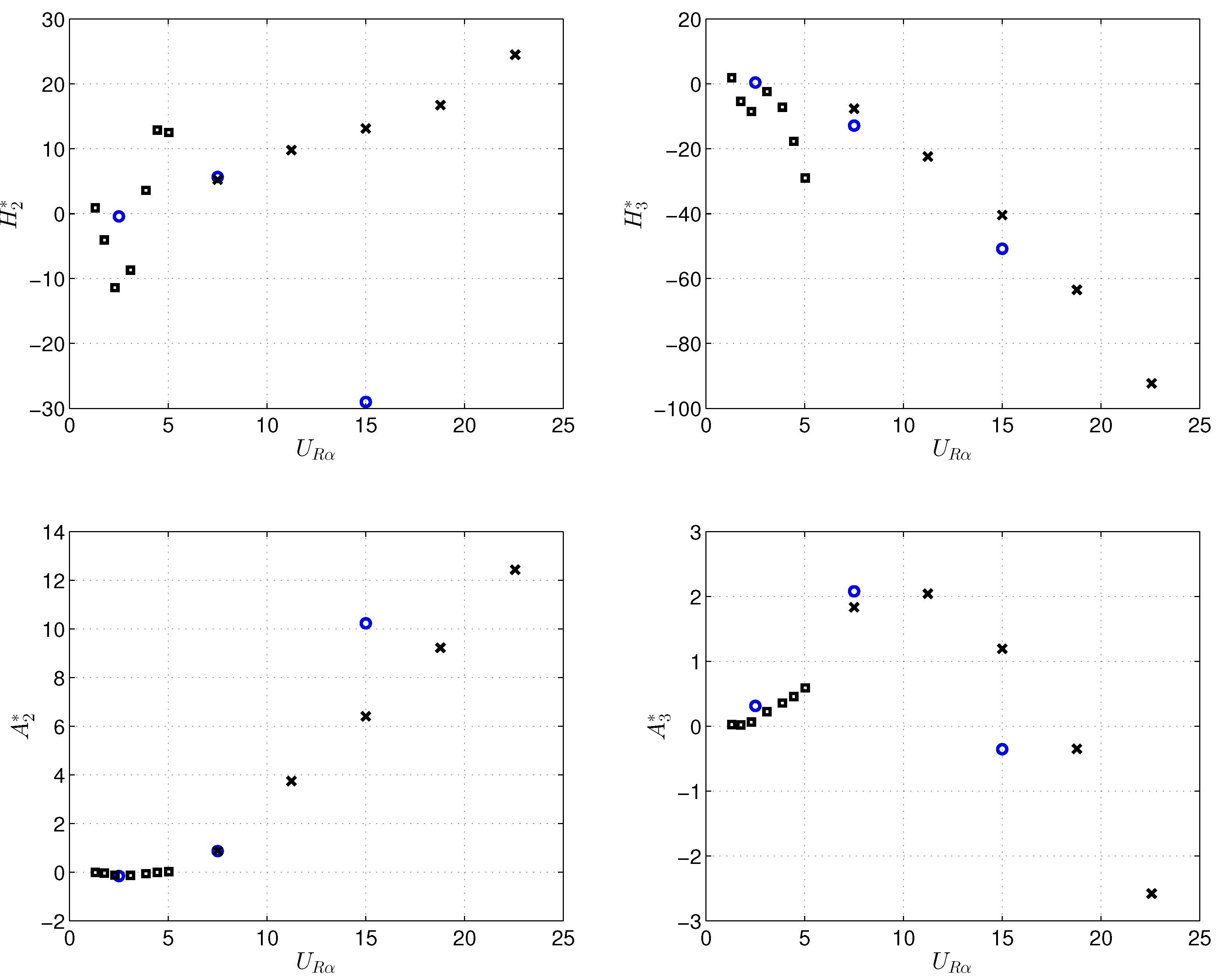
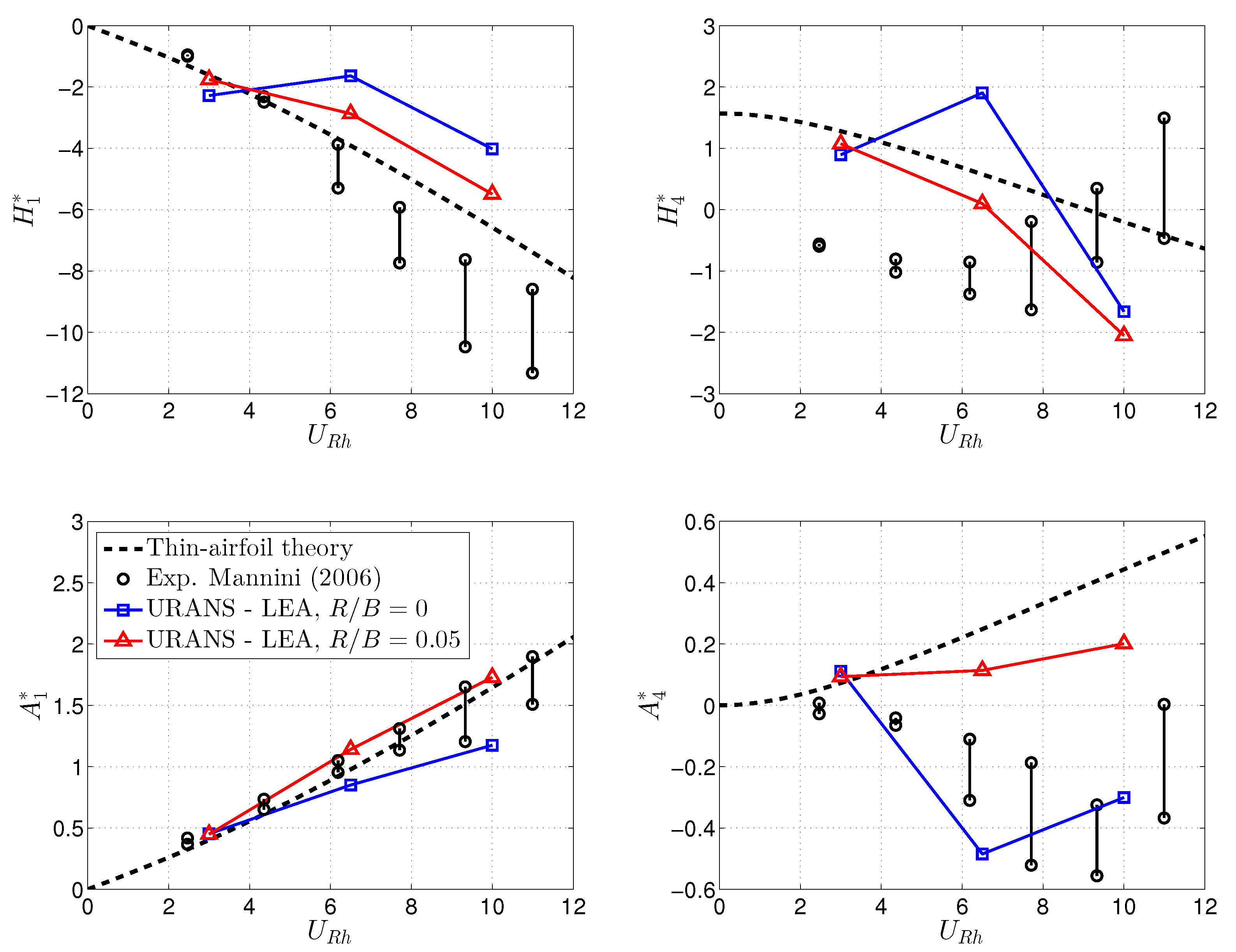
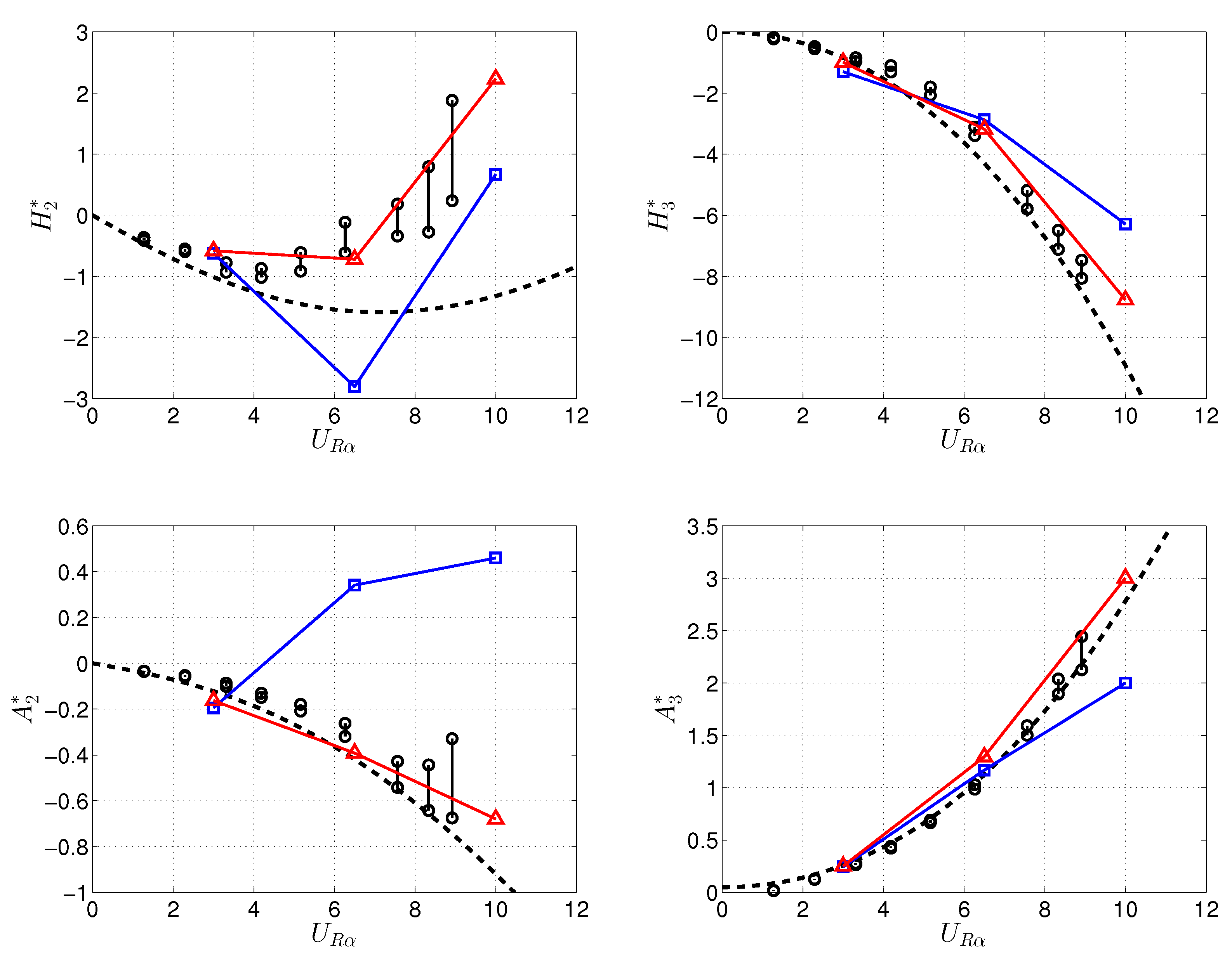
4.2. Flutter Derivatives


5. Conclusions
- The 2D URANS approach combined with the EARSM-LEA turbulence model gives results of reasonable accuracy for the rectangular cylinders and the bridge section considered. In particular, complex phenomena, such as the Reynolds number effects observed in the wind tunnel for the sharp-edged rectangular 5:1 cylinder (), are qualitatively captured, although they result in being less pronounced than in the experiments.
- In the particular case of a rectangular 1:5 cylinder (), with the long side perpendicular to the flow, 3D simulations are necessary to obtain acceptable results, even with the URANS equations.
- Forced vibration simulations were carried out for the rectangular 5:1 cylinder with 2D URANS equations in combination with the eddy viscosity model of Spalart and Allmaras (SAE). The results are in overall good agreement with experiments, but significant improvements can be expected by adopting an EARSM turbulence model. In particular, the numerical calculations correctly predict the expected threshold of torsional galloping instability.
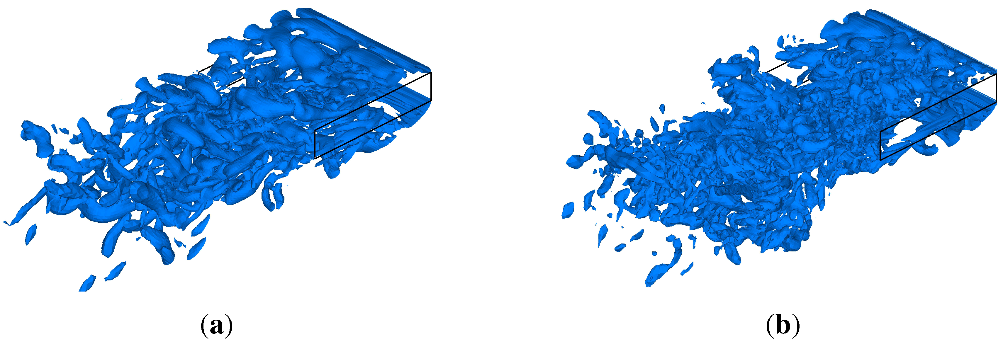
- The 3D DES-SA approach for the rectangular 5:1 cylinder delivers more accurate results than both the 2D and 3D URANS equations. Nevertheless, the study highlights that the results are sensitive to the amount of artificial dissipation introduced to stabilize the central difference discretization of the convective term in the governing equation.
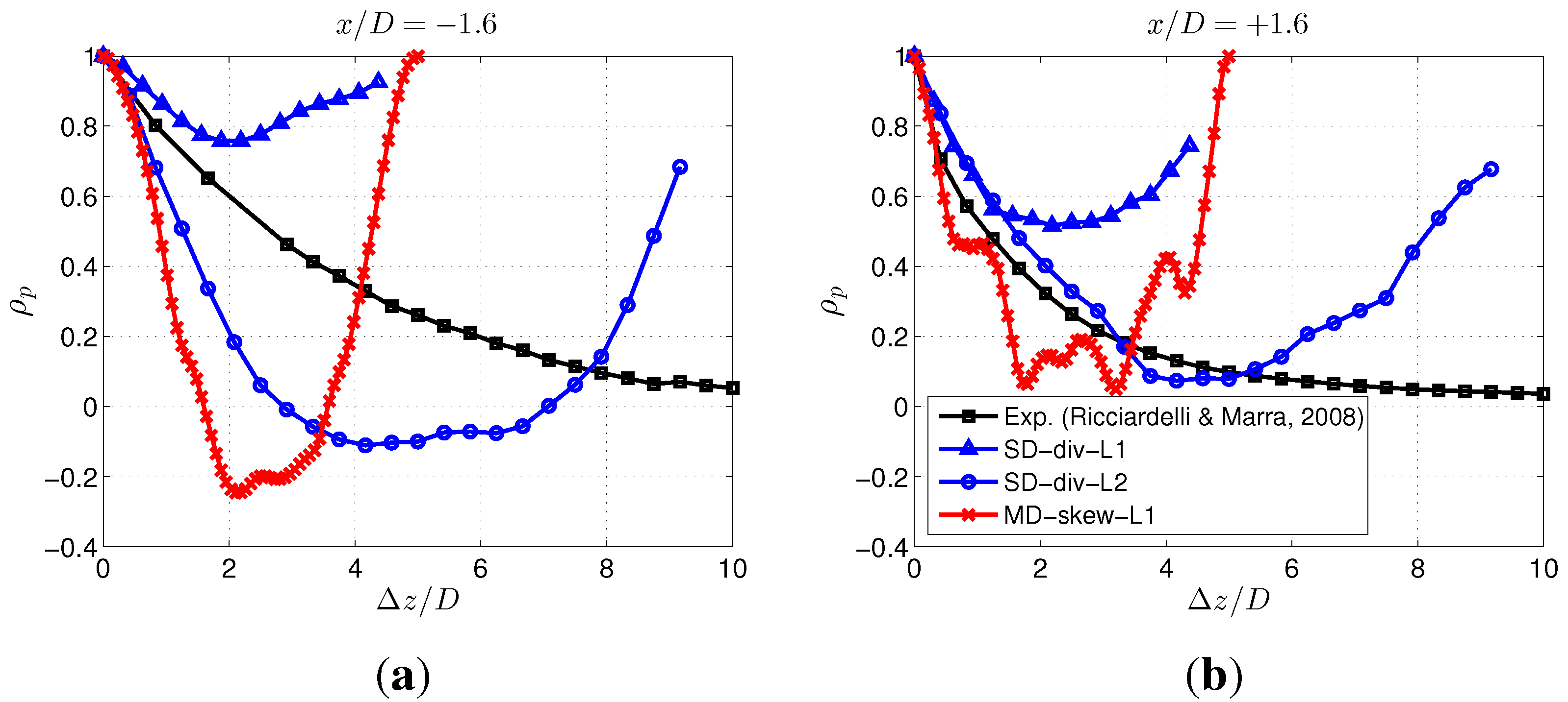
- A large spanwise extension of the computational domain is required in a 3D DES simulation to allow the natural loss of the correlation of the fluctuating pressure field.
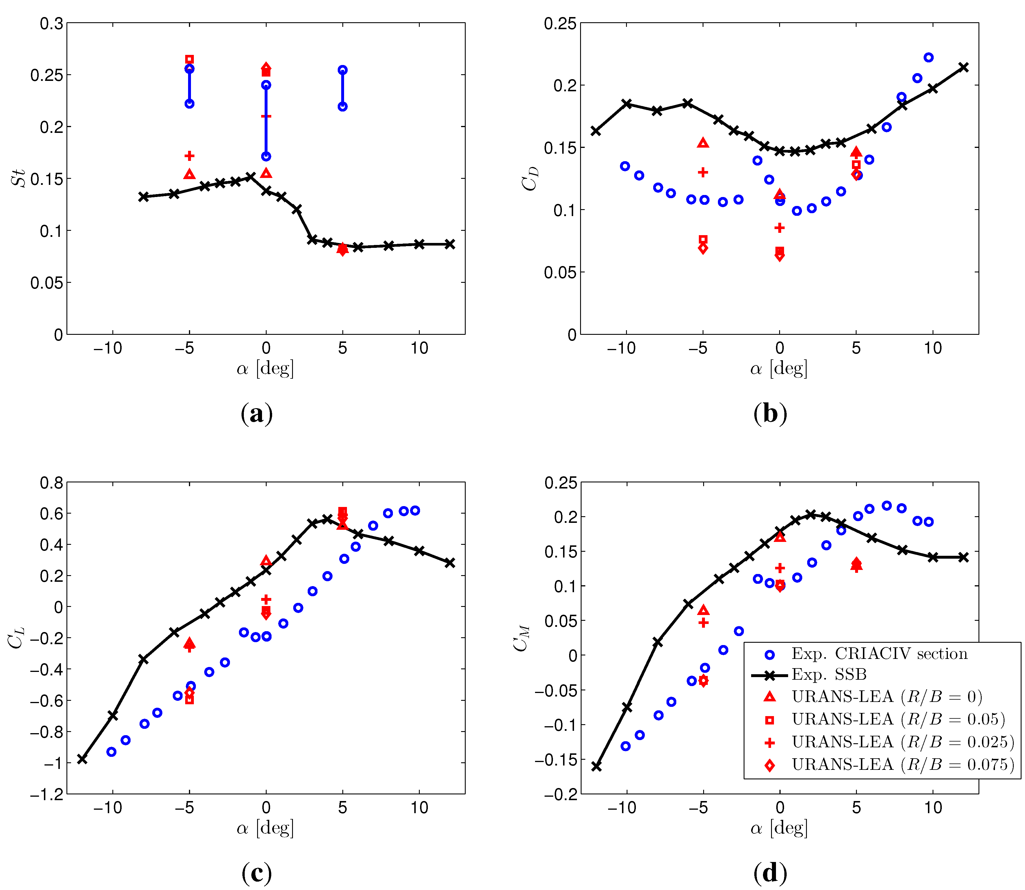
- 2D URANS-LEA numerical simulations of flow past a realistic bridge section give results in satisfactory agreement with experiments and helped to understand the discrepancy between two sets of experimental data available in the literature for two very similar geometries.
- The numerical results underscore the key role played by the degree of sharpness of the bridge section lower corners with respect to both static and aeroelastic behavior. In particular, the section is prone to low speed torsional galloping in the case of sharp edges, while higher speed coupled flutter is expected if the lower corners present a small radius of curvature.
Acknowledgments
Conflicts of Interest
References
- Schwamborn, D.; Gerhold, T.; Heinrich, R. The DLR-Tau code: Recent applications in research and industry. In Proceedings of the European Conference on Computational Fluid Dynamics, Delft, The Netherlands, 5–8 September 2006.
- Jameson, A.; Schmidt, W.; Turkel, E. Numerical solution of the Euler equations by finite volume methods using Runge Kutta time stepping schemes. In Proceedings of the AIAA 14th Fluid and Plasma Dynamics Conference, Palo Alto, CA, USA, 23–25 June 1981.
- Mavriplis, D.; Jameson, A.; Martinelli, L. Multigrid solution of the Navier-Stokes equations on triangular meshes. In Proceedings of the 27th AIAA Aerospace Sciences Meeting, Reno, NV, USA, 9–12 January 1989.
- Heinrich, R.; Dwight, R.; Widhalm, M.; Raichle, A. Algorithmic Developments in TAU. In MEGAFLOW—Numerical Flow Simulation for Aircraft Design, Notes on Numerical Fluid Mechanics and Multidisciplinary Design; Kroll, N., Fassbender, J.K., Eds.; Springer: Berlin/Heidelberg, Germany, 2005; Volume 89, pp. 93–108. [Google Scholar]
- Spalart, P.R.; Allmaras, S.R. A one-equation turbulence model for aerodynamic flows. In Proceedings of the 30th AIAA Aerospace Sciences Meeting and Exhibit, NV, USA, 6–9 January 1992.
- Edwards, J.R.; Chandra, S. Comparison of eddy viscosity-transport turbulence models for three-dimensional, shock-separated flowfields. AIAA J. 1996, 34, 756–763. [Google Scholar] [CrossRef]
- Menter, F.R. Two-equation k-ω turbulence model for aerodynamic flows. AIAA J. 1994, 32, 269–289. [Google Scholar] [CrossRef]
- Rodi, W. Turbulence modeling for boundary-layer calculations. In IUTAM Symposium on One Hundred Years of Boundary Layer Research; Meier, G.E.A., Sreenivasan, K.R., Eds.; Springer: Dordrecht, The Netherlands, 2006; pp. 247–256. [Google Scholar]
- Rung, T.; Bunge, U.; Schatz, M.; Thiele, F. Restatement of the Spalart–Allmaras eddy-viscosity model in strain-adaptive formulation. AIAA J. 2003, 41, 1396–1399. [Google Scholar] [CrossRef]
- Wilcox, D. Turbulence Modeling for CFD, 3rd ed.; DCW Industries, Inc.: La Cañada, CA, USA, 2006. [Google Scholar]
- Lübcke, H.; Schmidt, S.; Rung, T.; Thiele, F. Comparison of LES and RANS in bluff-body flows. J. Wind Eng. Ind. Aerodyn. 2001, 89, 1471–1485. [Google Scholar] [CrossRef]
- Rung, T.; Lübcke, H.; Franke, M.; Xue, L.; Thiele, F.; Fu, S. Assessment of Explicit Algebraic Stress Models in transonic flows. In Proceedings of the 4th International Symposium on Engineering Turbulence Modeling and Experiments, Ajaccio, France, 24–26 May 1999; pp. 659–668.
- Gatski, T.B.; Speziale, C.G. On explicit algebraic stress models for complex turbulent flows. J. Fluid Mech. 1993, 254, 59–78. [Google Scholar] [CrossRef]
- Wilcox, D. Reassessment of the scale-determining equation for advanced turbulence models. AIAA J. 1988, 26, 1299–1310. [Google Scholar] [CrossRef]
- Aupoix, B. Non linear eddy viscosity models and explicit algebraic Reynolds stress models. In FLOMANIA—A European Initiative on Flow Physics Modeling; Haase, W., Aupoix, B., Bunge, U., Schwamborn, D., Eds.; Springer: Berlin/Heidelberg, Germany, 2006; Volume 94, pp. 142–153. [Google Scholar]
- Spalart, P.R.; Jou, W.H.; Strelets, M.K.; Allmaras, S.R. Comments on the feasibility of LES for wings, and on a hybrid RANS/LES approach. In Advances in DNS/LES, Proceedings of the First AFOSR International Conference on DNS/LES, Louisiana Tech University, Ruston, LA, USA, 4–8 August 1997; pp. 137–147.
- Shur, M.L.; Spalart, P.R.; Strelets, M.K.; Travin, A. Detached-Eddy Simulation of an airfoil at high angle of attack. In Proceedings of the 4th International Symposium on Engineering Turbulence Modeling and Experiments, Ajaccio, France, 24–26 May 1999; pp. 669–678.
- Spalart, P.R. Young-Person’s Guide to Detached-Eddy Simulation Grids; Technical Report; CR-2001-211032; NASA Langley Research Center: Hampton, VA, USA, 2001. [Google Scholar]
- Strelets, M.K. Detached Eddy Simulation of massively separated flows. In Proceedings of the 39th AIAA Aerospace Sciences Meeting and Exhibit, Reno, NV, USA, 8–11 January 2001.
- Soda, A. Numerical Investigation of Unsteady Transonic Shock/Boundary-Layer Interaction for Aeronautical Applications. PhD Thesis, RWTH Aachen University, Aachen, Germany, 2006. [Google Scholar]
- Weinman, K.; van der Ven, H.; Mockett, C.; Knopp, T.; Kok, J.; Perrin, R.; Thiele, F. A study of grid convergence issues for the simulation of the massively separated flow around a stalled airfoil using DES and related methods. In Proceedings of the European Conference on Computational Fluid Dynamics, Delft, The Netherlands, 5–8 September 2006.
- Spalart, P.R.; Deck, S.; Shur, M.L.; Squires, K.D.; Strelets, M.K.; Travin, A.K. A new version of Detached-Eddy Simulation, resistant to ambiguous grid densities. Theor. Comput. Fluid Dyn. 2006, 20, 181–195. [Google Scholar] [CrossRef]
- Travin, A.K.; Shur, M.L.; Spalart, P.R.; Strelets, M.K. Improvement of Delayed Detached-Eddy Simulation for LES with wall modeling. In Proceedings of the European Conference on Computational Fluid Dynamics, Delft, The Netherlands, 5–8 September 2006.
- Weinman, K.; Knopp, T.; Schwamborn, D. Contributions of DLR in DESider. In DESider—A European Effort on Hybrid RANS-LES Modelling; Haase, W., Braza, M., Revell, A., Eds.; Springer: Berlin/Heidelberg, Germany, 2009; Volume 103, pp. 341–346. [Google Scholar]
- Kravchenko, A.G.; Moin, P. On the effect of numerical errors in Large Eddy Simulations of turbulent flow. J. Comput. Phys. 1997, 131, 310–322. [Google Scholar] [CrossRef]
- Whitfield, D.L.; Janus, J.M. Three-dimensional Unsteady Euler equations solution using flux vector splitting. In Proceedings of the 17th AIAA Fluid Dynamics, Plasma Dynamics, and Lasers Conference, Snowmass, CO, USA, 25–27 June 1984.
- Šoda, A.; Mannini, C.; Sjerić, M. Investigation of unsteady air flow around two-dimensional rectangular cylinders. Trans. Famena 2011, 35, 11–34. [Google Scholar]
- Najjar, F.M.; Vanka, P. Simulations of the unsteady separated flow past a normal flat plate. Int. J. Numer. Methods Fluids 1995, 21, 525–547. [Google Scholar] [CrossRef]
- Shur, M.L.; Spalart, P.R.; Squires, K.D.; Strelets, M.K.; Travin, A. Three dimensionality in Reynolds-Averaged Navier-Stokes solutions around two-dimensional geometries. AIAA J. 2005, 43, 1230–1242. [Google Scholar] [CrossRef]
- Nakamura, Y.; Ohya, Y. The effects of turbulence on the mean flow past two-dimensional rectangular cylinders. J. Fluid Mech. 1984, 149, 255–273. [Google Scholar] [CrossRef]
- Shimada, K.; Ishihara, T. Application of a modified k-ϵ model to the prediction of aerodynamic characteristics of rectangular cross-section cyliders. J. Fluids Struct. 2002, 16, 465–485. [Google Scholar] [CrossRef]
- Schewe, G. Untersuchung der aerodynamischen Kräfte, die auf stumpfe Profile bei großen Reynolds-Zahlen wirken; Technical Report; DFVLR-Mitt. 84-19; Institut für Aeroelastik: Göttingen, Germany, 1984. (In German) [Google Scholar]
- Lyn, D.A.; Einav, S.; Rodi, W.; Park, J.H. A laser Doppler velocimetry study of ensemble-averaged characteristics of the turbulent flow near wake of a square cylinder. J. Fluid Mech. 1995, 304, 285–319. [Google Scholar] [CrossRef]
- Rodi, W. Comparison of LES and RANS calculations of the flow around bluff bodies. J. Wind Eng. Ind. Aerodyn. 1997, 69–71, 55–75. [Google Scholar] [CrossRef]
- Okajima, A. Strouhal numbers of rectangular cylinders. J. Fluid Mech. 1982, 123, 379–398. [Google Scholar] [CrossRef]
- Matsumoto, M.; Shirato, H.; Araki, K.; Haramura, T.; Hashimoto, T. Spanwise coherence characteristics of surface pressure field on 2-D bluff bodies. J. Wind Eng. Ind. Aerodyn. 2003, 91, 155–163. [Google Scholar] [CrossRef]
- Schewe, G. Reynolds-number-effects in flow around a rectangular cylinder with aspect ratio 1:5. J. Fluids Struct. 2013, 39, 15–26. [Google Scholar] [CrossRef]
- Mannini, C.; Marra, A.M.; Pigolotti, L.; Bartoli, G. Unsteady pressure and wake characteristics of a benchmark rectangular section in smooth and turbulent flow. In Proceedings of the 14th International Conference on Wind Engineering, Porto Alegre, Brazil, 21–26 June 2015.
- Bartoli, G.; Bruno, L.; Buresti, G.; Ricciardelli, F.; Salvetti, M.V.; Zasso, A. BARC Overview Document. Available online: http://www.aniv-iawe.org/barc (accessed on 17 September 2015).
- Mannini, C.; Šoda, A.; Schewe, G. Unsteady RANS modeling of flow past a rectangular cylinder: Investigation of Reynolds number effects. Comput. Fluids 2010, 39, 1609–1624. [Google Scholar] [CrossRef]
- Mannini, C.; Soda, A.; Voss, R.; Schewe, G. URANS and DES simulation of flow around a rectangular cylinder. In New Results in Numerical and Experimental Fluid Mechanics VI; Tropea, C., Jakirlic, S., Heinemann, H.J., Henke, R., Hönlinger, H., Eds.; Springer: Berlin/Heidelberg, Germany, 2008; Volume 96. [Google Scholar]
- Scanlan, R. The action of flexible bridges under wind, I: Flutter theory. J. Sound Vib. 1978, 60, 187–199. [Google Scholar] [CrossRef]
- Matsumoto, M. Aerodynamic damping of prisms. J. Wind Eng. Ind. Aerodyn. 1996, 59, 159–175. [Google Scholar] [CrossRef]
- Righi, M. Aeroelastic Stability of Long Span Suspended Bridges: Flutter Mechanism on Rectangular Cylinders in Smooth and Turbulent Flow. Ph.D. Thesis, University of Florence, Florence, Italy, 1996. [Google Scholar]
- Mannini, C.; Šoda, A.; Schewe, G. Numerical investigation on the three-dimensional unsteady flow past a 5:1 rectangular cylinder. J. Wind Eng. Ind. Aerodyn. 2011, 99, 469–482. [Google Scholar] [CrossRef]
- Mannini, C.; Schewe, G. Detached-eddy simulations of a Benchmark on the Aerodynamics of a Rectangular 5:1 Cylinder. In Proceedings of the 20th Congress of the Italian Association of Theoretical and Applied Mechanics, Bologna, Italy, 12–15 September 2011.
- Camarri, S.; Salvetti, M.V.; Koobus, B.; Dervieux, A. A low-diffusion MUSCL scheme for LES on unstructured grids. Comput. Fluids 2004, 33, 1101–1129. [Google Scholar] [CrossRef]
- Bruno, L.; Fransos, D.; Coste, N.; Bosco, A. 3D flow around a rectangular cylinder: A computational study. J. Wind Eng. Ind. Aerodyn. 2010, 98, 263–276. [Google Scholar] [CrossRef]
- Matsumoto, M.; (Kyoto University, Kyoto, Japan). Personal communication, 2005.
- Galli, F. Comportamento Aerodinamico di Strutture Snelle Non Profilate: Approccio Sperimentale e Computazionale. Master’s Thesis, Politecnico di Torino, Turin, Italy, 2005. [Google Scholar]
- Bronkhorst, A.J.; Geurts, C.P.W.; van Bentum, C.A. Unsteady pressure measurements on a 5:1 rectangular cylinder. In Proceedings of the 13th International Conference on Wind Engineering, Amsterdam, The Netherlands, 10–15 July 2011.
- Lander, D.C.; Baker, J.; Letchford, C.W.; Amitay, M.; Kopp, G.A. The effect of freestream turbulence on vortex formation in the wake of a square cylinder. In Proceedings of the 14th International Conference on Wind Engineering, Porto Alegre, Brazil, 21–26 June 2015.
- Bruno, L.; Coste, N.; Fransos, D. Simulated flow around a rectangular 5:1 cylinder: Spanwise discretisation effects and emerging flow features. J. Wind Eng. Ind. Aerodyn. 2012, 104–106, 203–215. [Google Scholar] [CrossRef]
- Ricciardelli, F.; Marra, A.M. Sectional aerodynamic forces and their longitudinal correlation on a vibrating 5:1 rectangular cylinder. In Proceedings of the 6th International Colloquium on Bluff Body Aerodynamics and Applications, Milan, Italy, 20–24 July 2008.
- Mannini, C. Flutter Vulnerability Assessment of Flexible Bridge Decks. Ph.D. Thesis, University of Florence, Florence, Italy, TU Braunschweig, Braunschweig, Germany, 2006; Verlag Dr. Müller, Saarbrücken, Germany, 2008.
- Ricciardelli, F.; Hangan, H. Pressure distribution and aerodynamic forces on stationary box bridge sections. Wind Struct. 2001, 4, 399–412. [Google Scholar] [CrossRef]
- Mannini, C.; Šoda, A.; Voß, R.; Schewe, G. Unsteady RANS simulations of flow around a bridge section. J. Wind Eng. Ind. Aerodyn. 2010, 98, 742–753. [Google Scholar] [CrossRef]
- Sarwar, M.; Ishihara, T.; Shimada, K.; Yamasaki, Y.; Ikeda, T. Prediction of aerodynamic characteristics of a box girder bridge section using the LES turbulence model. J. Wind Eng. Ind. Aerodyn. 2008, 96, 1895–1911. [Google Scholar] [CrossRef]
- Bai, Y.; Sun, D.; Lin, J. Three dimensional numerical simulations of long-span bridge aerodynamics, using block-iterative coupling and DES. Comput. Fluids 2010, 39, 1549–1561. [Google Scholar] [CrossRef]
- Šarkić, A.; Fisch, R.; Höffer, R.; Bletzinger, K.U. Bridge flutter derivatives based on computed, validated pressure fields. J. Wind Eng. Ind. Aerodyn. 2012, 104–106, 141–151. [Google Scholar] [CrossRef]
- Brusiani, F.; de Miranda, S.; Patruno, L.; Ubertini, F.; Vaona, P. On the evaluation of bridge deck flutter derivatives using RANS turbulence models. J. Wind Eng. Ind. Aerodyn. 2013, 119, 39–47. [Google Scholar] [CrossRef]
- Mannini, C.; Bartoli, G. Aerodynamic uncertainty propagation in bridge flutter analysis. Struct. Saf. 2015, 52, 29–39. [Google Scholar] [CrossRef]
- Mannini, C.; Sbragi, G.; Schewe, G.; Borri, C. Determination of flutter derivatives for a box-girder bridge deck through URANS simulations. In Proceedings of the 8th International Conference on Structural Dynamics, Leuven, Belgium, 4–6 July 2011.
- Mannini, C.; Sbragi, G.; Schewe, G. Analysis of self-excited forces for a box-girder bridge deck through unsteady RANS simulations. J. Fluids Struct. 2015. submitted. [Google Scholar]
- Ricciardelli, F. On the wind loading mechanism of long-span bridge deck box sections. J. Wind Eng. Ind. Aerodyn. 2003, 91, 1411–1430. [Google Scholar] [CrossRef]
© 2015 by the authors; licensee MDPI, Basel, Switzerland. This article is an open access article distributed under the terms and conditions of the Creative Commons Attribution license (http://creativecommons.org/licenses/by/4.0/).
Share and Cite
Mannini, C. Applicability of URANS and DES Simulations of Flow Past Rectangular Cylinders and Bridge Sections. Computation 2015, 3, 479-508. https://doi.org/10.3390/computation3030479
Mannini C. Applicability of URANS and DES Simulations of Flow Past Rectangular Cylinders and Bridge Sections. Computation. 2015; 3(3):479-508. https://doi.org/10.3390/computation3030479
Chicago/Turabian StyleMannini, Claudio. 2015. "Applicability of URANS and DES Simulations of Flow Past Rectangular Cylinders and Bridge Sections" Computation 3, no. 3: 479-508. https://doi.org/10.3390/computation3030479