On Roof Geometry for Urban Wind Energy Exploitation in High-Rise Buildings

Abstract

The European program HORIZON2020 aims to have 20% of electricity produced by renewable sources. The building sector represents 40% of the European Union energy consumption. Reducing energy consumption in buildings is therefore a priority for energy efficiency. The present investigation explores the most adequate roof shapes compatible with the placement of different types of small wind energy generators on high-rise buildings for urban wind energy exploitation. The wind flow around traditional state-of-the-art roof shapes is considered. In addition, the influence of the roof edge on the wind flow on high-rise buildings is analyzed. These geometries are investigated, both qualitatively and quantitatively, and the turbulence intensity threshold for horizontal axis wind turbines is considered. The most adequate shapes for wind energy exploitation are identified, studying vertical profiles of velocity, turbulent kinetic energy and turbulence intensity. Curved shapes are the most interesting building roof shapes from the wind energy exploitation point of view, leading to the highest speed-up and the lowest turbulence intensity.

1. Introduction

It is well known that wind energy drastically reduces carbon emissions and avoids geo-political risks associated with supply and infrastructure constraints, as well as energy dependence from other regions. The HORIZON2020 Research and Innovation Programme [1] in Future Smart Cities aims to have 20% of electricity produced by renewable sources. This goal stresses the necessity to improve and optimize wind energy generation, both with large- and small-scale wind turbines.

Large-scale wind turbines are very efficient when they are placed in large wind farms. The efficient placement of smaller scale wind turbines in the urban environment is a largely unexplored area. This implies a waste of an important energy resource [2,3]. One of the potential outcomes of optimized wind farm layouts in an urban environment is distributed energy generation (generation at the consumption site), which offers significant benefits in terms of high energy efficiency, lower emissions of pollutants, reduced energy dependence and stimulation of the economy [4]. The main reasons for the waste of urban wind energy resources are the lack of studies focused on resource availability assessment and a certain lack of societal acceptance. The main objective of the COST Action TU1304 [5] study is to collect the existing expertise on building-integrated wind energy technology and to investigate effective adoption methods for enabling the concept of a smart future city. The dissemination is focused in particular on the societal acceptance. One of the most significant aspects of this lack of societal acceptance is due to customers’ disappointment regarding the difference between the expected and the real energy generated. This difference occurs because the performances of the wind turbines are calculated under ideal conditions in flat terrain, conditions very different from the real conditions in the urban environment [6]. Another important aspect for social acceptance is the visual impact [5], which can be avoided by considering the wind turbines during the architectural design process.

The building sector represents 40% of the European Union’s (EU) total energy consumption. Reducing energy consumption in this area is therefore a priority under the “20-20-20” objectives on energy efficiency [7]. The Directive 2010/31/EU of the European Parliament and of the Council of 19 May 2010 on the energy performance of buildings [8] aims to contribute to this objective by proposing guiding principles for Member States regarding the energy performance of buildings. One of these guidelines concerns the minimum requirements for energy efficiency during the design of new buildings. New buildings shall comply with these requirements and undergo a feasibility study before construction starts, looking at the installation of renewable energy supply systems and other sustainable systems [8], such as wind energy exploitation devices. New software [9] is being developed nowadays for the evaluation of wind energy resources in the urban environment.

Toja-Silva et al. [6] present a review of the opportunities and challenges of urban wind energy that stresses the necessity to perform accurate analyses of the flow behavior on building roofs, in order to get more information about possible positions of wind turbines to take advantage of the accelerating effect of the wind above the building, the adequate kind of turbine and the estimation of the power generation. Several authors [10–12] describe the influence of sharp building roof shapes on both the wind velocity and turbulence intensity from results obtained using computational fluid dynamics (CFD) simulations. These kinds of studies are essential for determining the most appropriate building shape and the optimal location and wind turbine model [13]. In these studies, four types of roof shape were analyzed: flat, shed, pitched and pyramidal. The results showed that, considering both velocity distributions and turbulence intensity, flat roofs were more attractive for installing wind turbines [10]. Shed roofs were also interesting, and a wind turbine could be installed on the top edge, because both high velocities and low turbulence intensities were present [11]. Abohela [14] demonstrated the interest in both vaulted and spherical roofs because of the lower turbulence and the speed-up factor. Although they are infrequently used, curved shapes present a clear advantage for wind energy exploitation.

The present study aims to identify the most adequate basic geometrical shapes that maximize the speed-up and minimize the turbulence intensity on high-rise (buildings higher than 23–30 m or 5–10 stories [15]) building roofs, for the purpose of urban wind energy exploitation. In the following, turbulence modeling, computational settings and validation are presented in Section 2. The state-of-the-art roof shapes are analyzed in Section 3. The influence of the roof edge shape on the wind flow is explained in Section 4, and the conclusions are in Section 5.

2. Turbulence Modeling and Computational Tools Validation

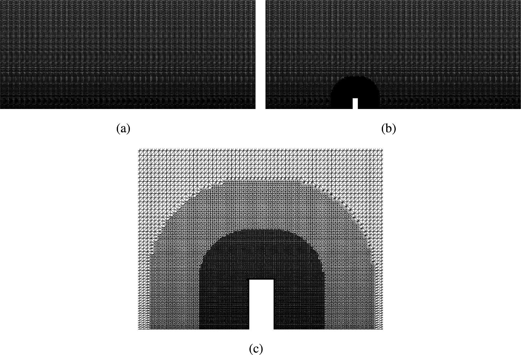
2.1. Governing Equations, Turbulence Modeling and Computational Settings

We use in the present investigation the steady-state Reynolds averaged Navier–Stokes (RANS) equations [16]. In addition, the steady-state equations for turbulent kinetic energy $(k=\frac{1}{2}\overline{{u^{\prime }}_i{u^{\prime }}_i})$ and turbulence dissipation (ε) without considering buoyancy are:

$$\frac{\partial ({\overline{u}}_{j}k)}{\partial x_j}=\frac{\partial }{\partial x_j}\left[\left(\nu +\frac{{\nu }_t}{{\sigma }_k}\right)\frac{\partial k}{\partial x_j}\right]+P_k-\epsilon$$

(1)

and:

$$\frac{\partial ({\overline{u}}_j\epsilon )}{\partial x_j}=\frac{\partial }{\partial x_j}\left[\left(\nu +\frac{{\nu }_t}{{\sigma }_{\epsilon }}\right)\frac{\partial \epsilon }{\partial x_j}\right]+C_{\epsilon 1}\frac{\epsilon }{k}{P}_k-C_{\epsilon 2}\frac{{\epsilon }^2}{k}$$

(2)

where σ_k and σ_ε (Prandtl numbers); C_ε1 and C_ε2 are closure constants; and P_k is the production of k:

$$P_k={\nu }_t{S}^2$$

(3)

where S is the modulus of the rate of strain tensor. The relationship between ν_t and the turbulence velocity time scale (T) is:

$${\nu }_t=C_{\mu }kT$$

(4)

where C_µ is a model coefficient for the turbulence model and T_SKE = k/ε is adopted for the standard k − ε (SKE) turbulence model. With the aim of reducing the overestimation of k on the impingement wall of bluff bodies, Durbin [17] proposed a bound in this time scale,

$$T=\min (T_{SKE},T_D)$$

(5)

This bounding can be modified in order to obtain a better agreement with experimental data, and some authors have used slightly different expressions. Toja-Silva et al. [18] have empirically found the following expression to obtain the good agreement of the recirculation distance on the building roof with the experimental data of [19]:

$$T_D=\frac{32}{45C_{\mu }S}$$

(6)

This turbulence model is used in all of the simulations of the present investigation. The coefficients in the equations are those proposed by Crespo et al. [20]: C_µ = 0.0333, C_ε1 = 1.176, C_ε2 = 1.92, σ_k = 1.0, σ_ε = 1.3 and κ = 0.42. These coefficients were obtained by Crespo et al. [20] from the atmospheric measurements of Panofsky and Dutton [21].

The steady-state simpleFoam solver for incompressible turbulent flow is used to solve the RANS equations in OpenFOAM [22]. For the spatial discretization of differential operators, Gaussian integration is used with different interpolation schemes. Second order linear interpolation is used for gradient terms, second order linear upwind interpolation for divergence terms and second order linear interpolation with explicit non-orthogonal correction for the Laplacian terms. Regarding the linear system solvers, generalized geometric-algebraic multi-grid solver (GAMG) with the diagonal incomplete-Cholesky (DIC) smoother is used for the pressure, and the preconditioned bi-conjugate gradient solver for asymmetric matrices (PBiCG) with the diagonal incomplete LU (DILU) preconditioner is used for the rest of the variables. The convergence criteria is set to 10⁻⁵ for all of the variables’ residuals.

We have successfully validated the modified Durbin turbulence model used in this investigation in Toja-Silva et al. [18] by studying the benchmark Case A of the Architectural Institute of Japan [23]. This benchmark case is an isolated building of an aspect ratio of 1:1:2 placed within an atmospheric boundary layer wind tunnel, tested by Meng and Hibi [19]. The recirculation distance on the roof found in the experiment was well matched by the simulations, and hit rates of HR_U = 87.5% and HR_k = 75.0% were obtained [18]. Additionally, we carried out a careful grid convergence analysis using three different meshes: fine (9.8 M cells), medium-sized (3.1 M) and coarse (1.7 M) mesh. We have obtained a convergence rate of 2.23 and a grid convergence index of 0.0577 (5.77%). See Toja-Silva et al. [18] for more details about both validation and grid convergence analysis and for a deeper discussion about how the modified Durbin model (Equation (6)) was derived.

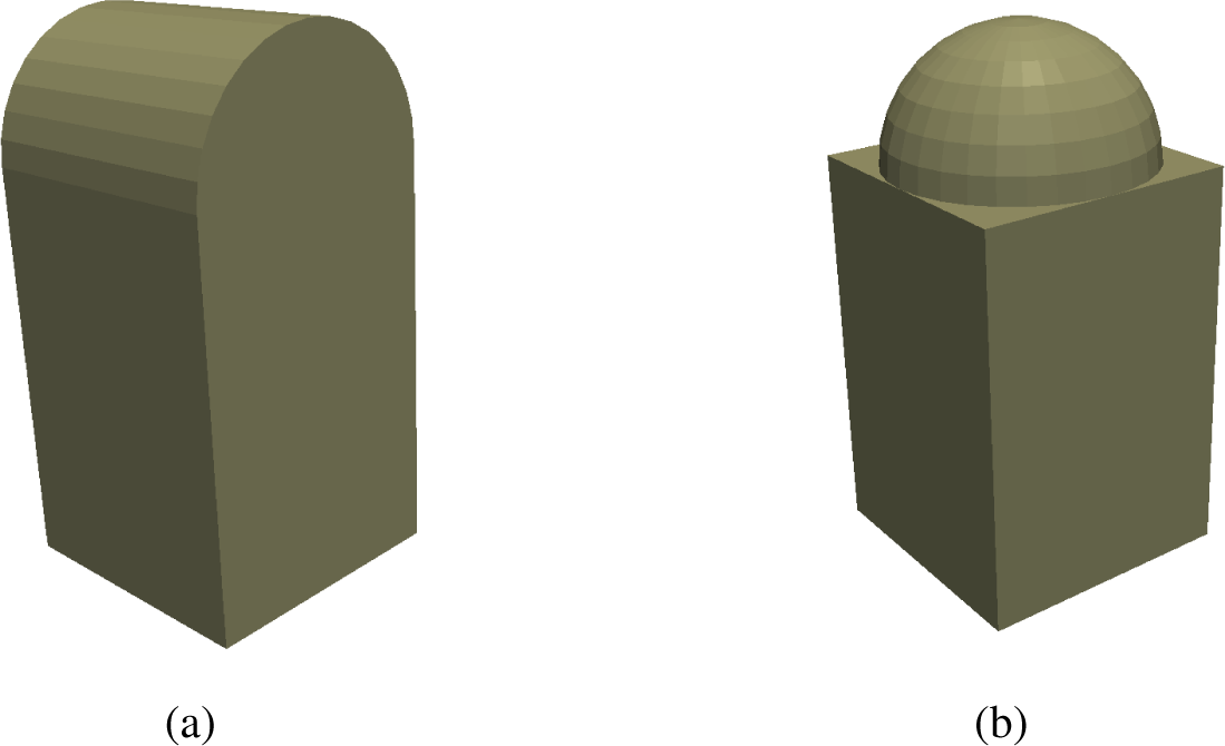
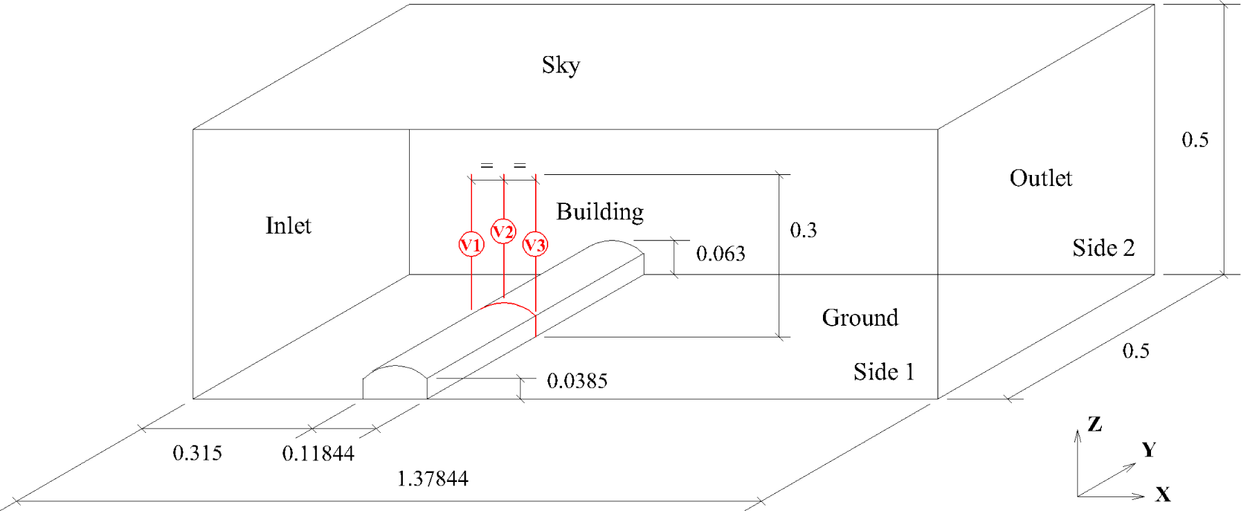
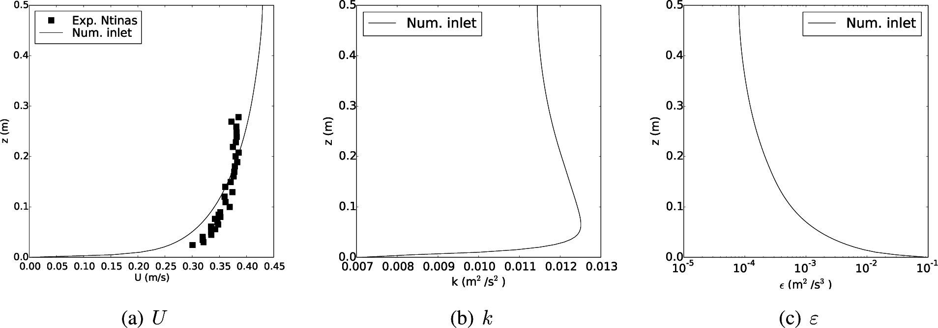
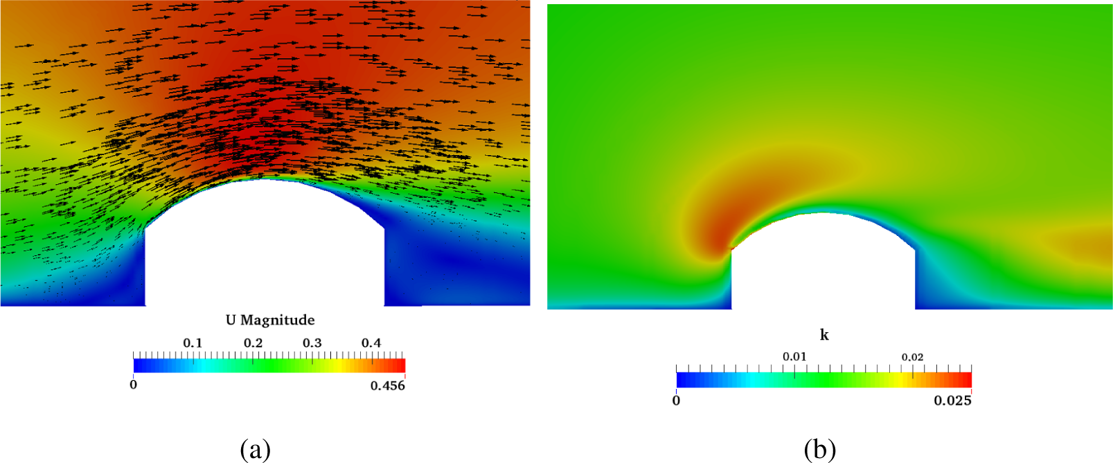
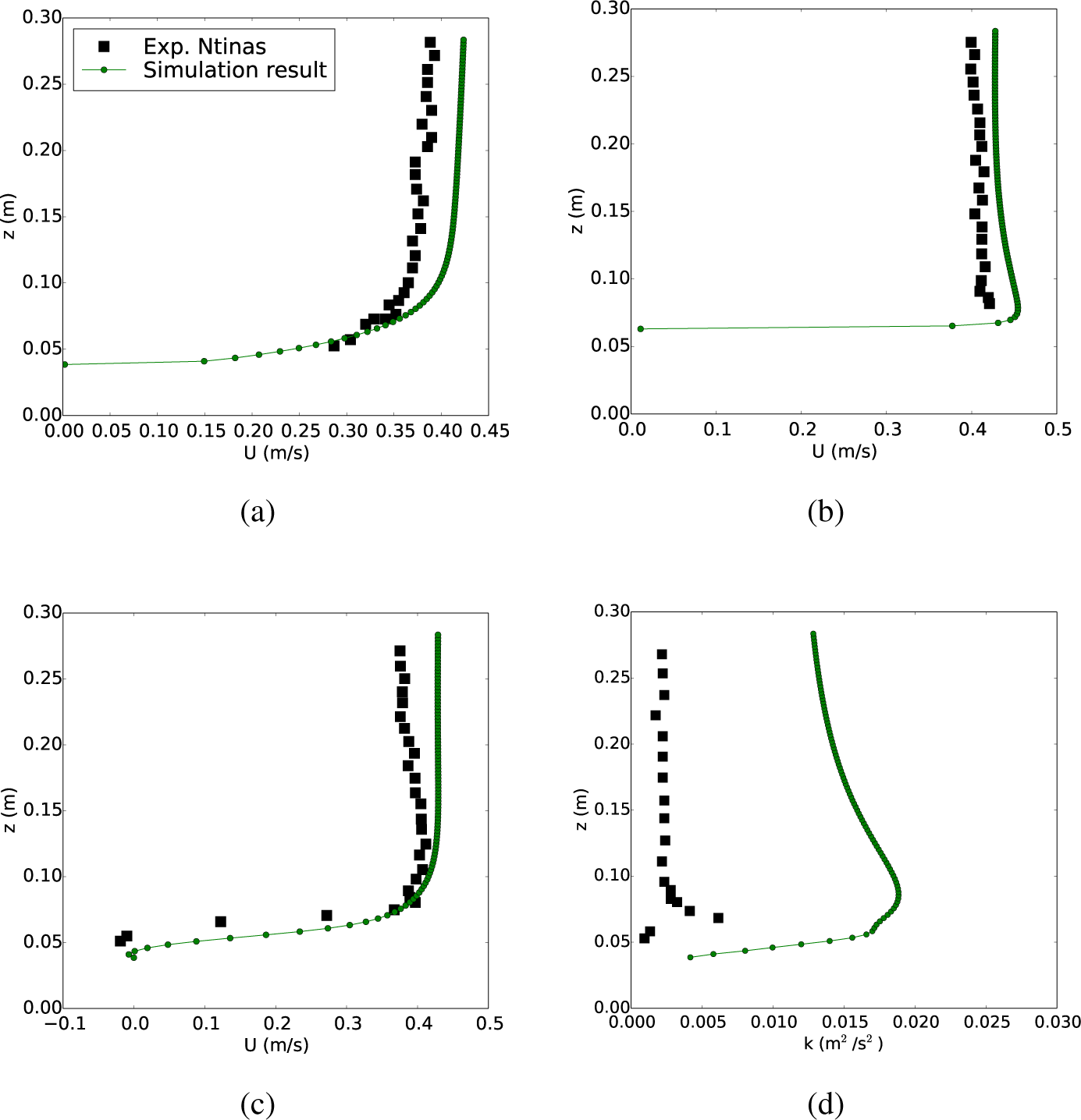
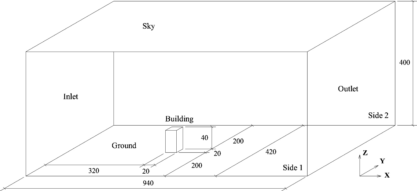
2.2. Additional Validation of Numerical Schemes Using a Curved Roof Model in Wind Tunnel

The modified Durbin k −ε turbulence model, tested on a flat roof in Toja-Silva et al. [18], is validated twice by comparing simulation results with those obtained from the wind tunnel experiment carried out by Ntinas et al. [24].

The geometry of the problem is the same as the wind-tunnel experiment of Ntinas et al. [24], and it is shown in detail in Figure 1. The building has a curved roof, and its transverse length is infinite (the whole transverse domain).

Table 1. Boundary conditions imposed at each boundary of the domain. Nomenclature: C = calculated; fV = fixed value; iP = inlet profile; sl = slip; sP = symmetry plane; wF = wall function; zG = zero gradient.

	U	k	ε	νt	p
Inlet	iP	iP	iP	C	zG
Outlet	zG	zG	zG	C	fV zero
Ground	fV zero	kqRwF	epsilon wF	nutkrough wF	zG
Building	fV zero	kqR wF	epsilon wF	nutk wF	zG
Sky	sl	sl	sl	C	zG
Sides	sP	sP	sP	sP	sP

presents the boundary conditions imposed for all of the variables at each boundary of the simulation domain.

The physical properties of the air used in the present case are ρ = 1.2 kg·m⁻³ and ν = 1.57 × 10⁻⁵ m²·s⁻¹.

The developed inlet wind profiles used for U, k and ε are shown in Figure 2. Since we calculate the inlet wind profiles of the full-scale simulations according to Richards and Hoxey [25], we use also this methodology in order to validate it by comparing the simulation results with the experimental data obtained by Ntinas et al. [24]. We consider the reference values used in the experiment: averaged wind velocity (U) inlet and the turbulent kinetic energy reference value of k = 0.011264 m²·s⁻². Notice that we use the logarithmic inlet wind profile for U (according to Richards and Hoxey [25]) instead of the exponential profile reported from the experiment (see Figure 2a). Since values of ε are not reported from the experiment, the entire inlet wind profile (Figure 2c) is defined according to Richards and Hoxey [25]. As is shown below, the validation is successful, and the agreement between the simulation results and the experimental values is reasonably good.

A background mesh is constructed with a grading of four in the vertical direction, and the building geometry is embedded into the background mesh. The refinement distance around the building surfaces is 0.1 m. Figure 3 shows the final mesh obtained.

Figure 4 shows U and k fields around the building roof. A small recirculation vortex appears at the down corner (between the wall and the ground) of the impingement wall, and a strong vortex appears downstream. This downstream vortex starts from the detached flow on the roof, which takes place at the center-downstream region. On the roof, k shows the highest values at the center-upstream region.

A quantitative analysis is carried out by comparing the numerical results for U and k with the experimental values of Ntinas et al. [24] on the vertical axes located at the central plane of the domain according to the diagram shown in Figure 1.

In order to provide a quantitative comparison of experimental and simulation results, we compute hit rates, a quantity widely used by the CFD research community, especially for atmospheric boundary layer flows [26–29]. The hit rates are calculated by using the equation:

$$HR=\frac{1}{n}{\displaystyle \sum _{i=1}^n{N}_i}$$

(7)

where n is the total number of points compared, and:

$$\begin{array}{l}{N}_i=1\text{if}\left|\frac{SI{M}_i-EX{P}_i}{EX{P}_i}\right|\le RD\text{or}|SI{M}_i-EX{P}_i|\le AD\\ N_i=0\text{else}\end{array}$$

(8)

where SIM_i and EXP_i are the simulation and experimental values and RD and AD are the relative and absolute maximum admissible deviation from the experimental data, respectively. These values are RD = 0.25 and AD = 0.05 and AD = 0.017 for U and k, respectively [18]. The values of the hit rate that allow considering the validation work as successful are HR ≥ 66%.

Figures 5a–c show a comparison of the vertical profiles of U at the roof positions V1, V2 and V3, respectively, described in Figure 1. Figure 5d shows a comparison of the vertical profiles of k at the vertical axis V3 (Figure 1), the only position with available experimental data. Since the experimental inlet profiles are not exactly reproduced and the Re number is low, both U an k are overestimated, although the turbulence model is successfully validated for both variables with hit rates of HR_U = 94.8% and HR_k = 100%. Note that the absolute difference between the values in Figure 5d is very small, although a clear overestimation is observed.

The results presented in this section show that the modified Durbin k − ε turbulence model used by Toja-Silva et al. [18], with the coefficients proposed by Crespo et al. [20], can provide a reasonable agreement with the experimental data in all cases studied. In what follows, we use this turbulence model to perform an accurate analysis of the wind flow on complex-geometry building roofs that include curved surfaces.

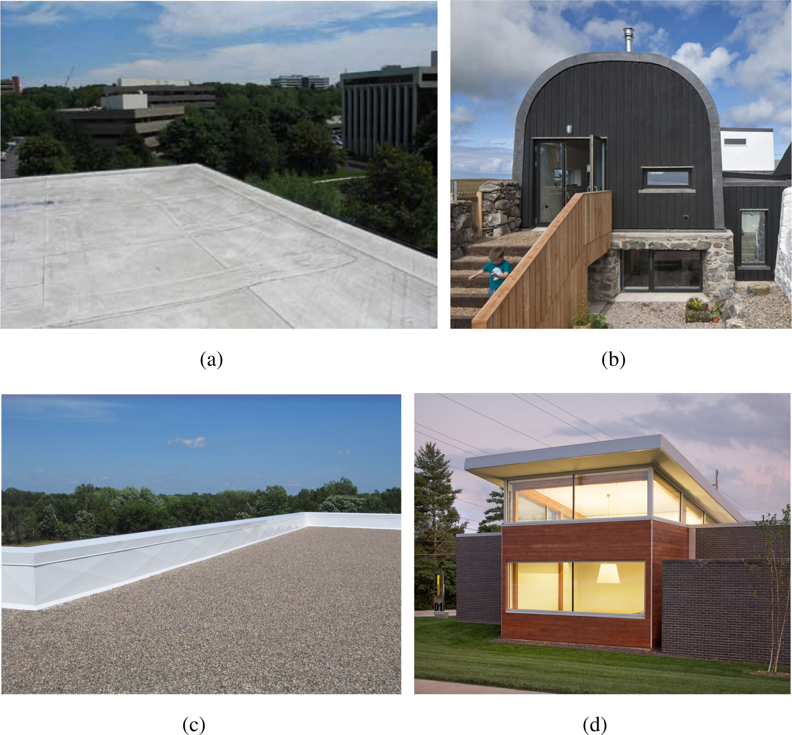
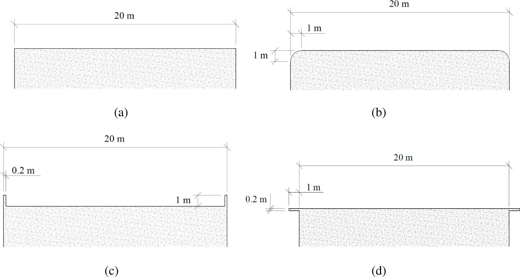
3. State-of-the-Art Roof Shapes

Five state-of-the-art roof shapes are tested in this section, specifically: flat, pitched, shed, spherical and vaulted roof shapes. The base-building is a squared-plant (20 × 20 m) building that is 40 m high. Figure 6 shows the domain and dimensions of the base building. The domain is set according to best practice guidelines [30]. According to Hall [31], Cowan et al. [32] and Scaperdas and Gilham [33], for a single building, a distance of 5H between the inflow boundary and the building is recommended if the approach flow profiles are well known. However, Bartzis et al. [34] recommends 8H if the inlet flow profiles are not available, as in the present case, in order to allow a realistic flow development.

Figure 7 shows a diagram of the different roof shapes investigated (note that the vertical section of spherical and vaulted roofs is the same). In this article, we test the spherical roof shape proposed by Abohela [14], a squared-plant building with a half sphere on the roof. Figure 8 shows the difference between the curved roofs, both vaulted and spherical.

As in the validation case, a background mesh with 3.3 M cells is constructed using the structured blockMesh application with a grading of four in the vertical direction and the building geometry, previously designed with a CAD tool and saved in stereolithography (STL) format. The geometry is embedded into this background mesh using the snappyHexMesh application of OpenFOAM [22,35,36]. The snappyHexMesh application is an adaptive refinement meshing utility of OpenFOAM that is very appropriate to mesh complex geometries, such as buildings with different shapes from STL CAD files. The mesh conforms to the building’s surface by iteratively refining (by splitting one original cell into four new ones) the background mesh and morphing the resulting split-hex mesh to the surface. The application allows one to define independent refinement boxes, but in the present case, the refinement is applied around the building surfaces. The refinement distance around the building surfaces is 80 m in this case. Figure 9 shows the background mesh used and the grid refinement set around the building in order to correctly reproduce the flow separation. These settings are used for all of the full-scale simulations performed in the present investigation.

Figure 10 shows a detailed view of the mesh, the number of mesh cells used and the averaged value of the non-dimensional wall distance (y⁺) at the roof shapes simulated (note that the vertical section of spherical and vaulted roofs is the same).

The boundary conditions imposed are shown in Table 1. The inlet profiles are calculated according to Richards and Hoxey [25], using the equations:

$$U=\frac{U_{\ast }}{\kappa }\ln \left(\frac{z+z_0}{z_0}\right)$$

(9)

$$\kappa =\frac{U_{\ast }^2}{\sqrt{C_{\mu }}}$$

(10)

and:

$$\epsilon =\frac{U_{\ast }^3}{\kappa (z+z_0)}$$

(11)

where z₀ = 0.01 m and U_ref = 4.4 m·s⁻¹ and z_ref = H = 40 m (H being the height of the building) are considered as reference values in order to calculate U_* by using Equation (9). Since 30 < y⁺ < 1000, we use standard turbulent wall laws [26,37,38] for the treatment of the near wall regions of the flow.

The quantitative results are analyzed by comparing U, k and turbulence intensity (TI) between the different cases at the vertical axis located at the most advantageous position at the central plane of the domain. This is on the upstream edge for the flat roof, on the downstream edge for the shed roof and on the center of the roof for the rest of the shapes investigated. Turbulence intensity is calculated as described in [39]:

$$TI=\frac{\sqrt{2k/3}}{U}$$

(12)

Figure 11a shows a comparison of the vertical profiles of U at the roof positions described above. The effect of the roof shape on U is appreciable at z/H < 1.50. Note that z/H is the dimensionless height from the ground, where z/H = 1.0 corresponds to the roof surface. Both shed and pitched shapes show a similar behavior: a decrease in U with a height up to z/H < 1.06. Above this height, U increases very slowly, until it reaches an almost constant value. The curved roofs cause a speed-up, with a concentration factor of the wind of around 30%. The highest value of U is observed for the vaulted roof. For the spherical roof, the maximum value of U is about 2.5% lower than the maximum value for the vaulted roof.

Figure 11b shows the comparison of vertical profiles of k at the roof positions described above. The effect of the edge shape on k is also appreciable at z/H < 1.35. All of the tested models significantly reduce the value of k with respect to the flat roof, and the peak value of k decreases by 63.8%. The spherical roof shows the lowest values in k, although the lower values at z/H < 1.05 are observed for shed and pitched roofs.

As is shown in Figure 11c, the effect of the different roof shapes on the wind flow is clearly appreciated at the height of the turbulence intensity limit for horizontal axis wind turbines (HAWT) of TI < 0.15 [18,40,41]. Compared with the flat roof, there is a moderate increase for pitched and shed roofs (15.2% and 26.6%, respectively), a moderate decrease for the vaulted roof (11.4%) and a significant decrease for the spherical roof (40.5%). The lower TI threshold is reached for the spherical roof, at z/H = 1.12. Below this TI threshold, vertical axis wind turbines (VAWT) may be considered due to their better behavior under skewed and highly turbulent flow conditions [3,6,42,43].

Figure 11d shows a comparison of the speed-up (U/U_ref) and the TI threshold height for the state-of-the-art cases at the roof positions described above. The most interesting cases from the wind energy exploitation point of view are at the low-right position in Figure 11d. They show the highest speed-up and lowest turbulence intensity. The most interesting cases are both vaulted and spherical. The vaulted shape generates a higher speed-up and the spherical a lower TI threshold height.

The results are qualitatively compared for both U and TI on the roof in Figures 12 and 13. The curved shapes (vaulted and spherical) generate a higher concentration factor that makes U even higher than the value of U several meters above the building. In the sharp cases (flat, pitched and shed), U is not horizontal at the highest speed position, an issue already highlighted in the literature [44]. This is important in order to correctly predict the potential energy yield and the fatigue loads on a machine [13,45–47]. For the flat roof, according to Toja-Silva et al. [18], the flow is skewed on the upstream roof edge around 5° at 0.19 < z/H < 0.31. Below this height, the inclination angle increases up to 40° close to the roof edge (z/H < 0.05). This value is also observed by Balduzzi et al. [12]. A flow inclination of 30° is observed for both pitched and shed roofs on the top. If HAWTs are used (above the TI threshold), the rotation axis of the wind turbine must be inclined according to the flow conditions (the power coefficient of a wind turbine with an incoming flow of 15° inclination decreases on average by 7% [48]). Additionally, VAWTs can be used with an skewed flow up to 25° [43]. The curved shapes generate an horizontal flow on the roof top, and the TI value decreases, particularly for the spherical shape.

The results show a similar behavior of the flow on the sharp (pitched and shed) and on the curved roofs (spherical and vaulted), respectively. The curved shapes (spherical and vaulted) generate a higher concentration factor of U. For the sharp cases (flat, pitched and shed), U is not horizontal at the highest speed position. Furthermore, the curved shapes significantly reduce the TI value, especially in the case of the spherical shape. The spherical roof has the additional advantage that it will generate the same flow (or very similar) for any incident wind direction. Therefore, among the simple geometric shapes tested, spherical and vaulted roofs are the best options from the wind energy exploitation point of view. An optimum building roof shape for the wind energy exploitation necessarily occurs by the use of curved shapes. A further step in this investigation must be the analysis of the wall to roof transition.

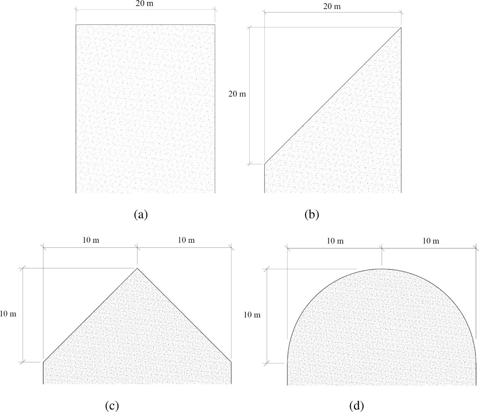
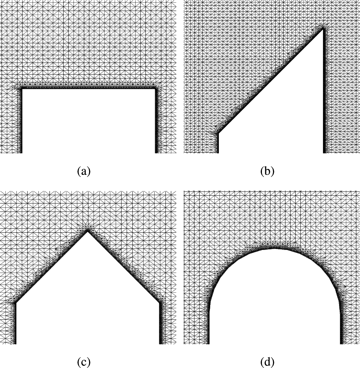
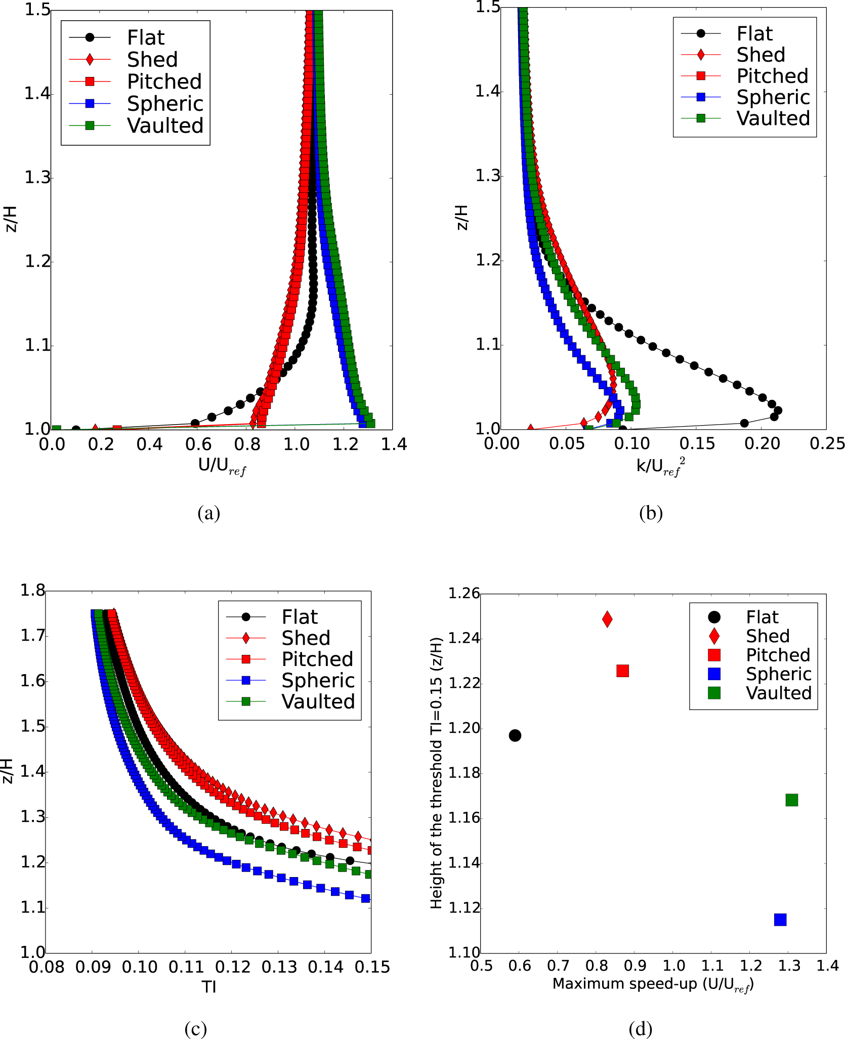
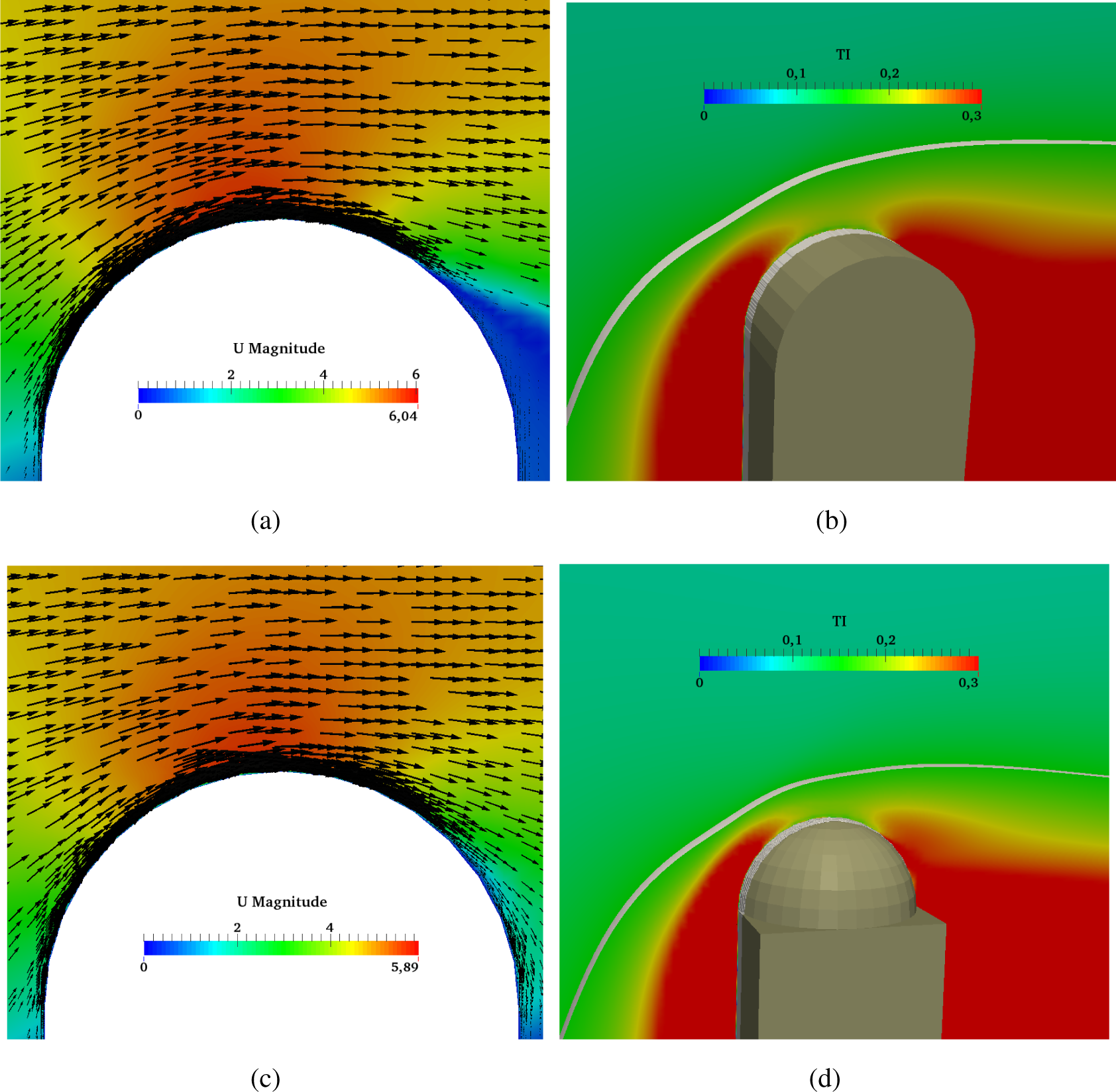
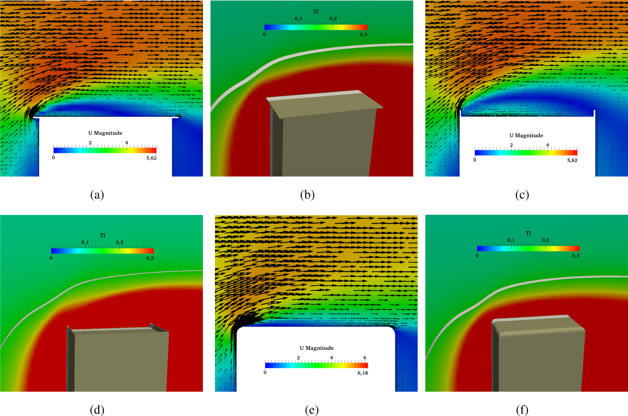
4. Influence of the Roof Edge Shape on the Wind Flow

The investigation of the influence of the roof edge shape on the wind flow is carried out by comparing the results obtained for a simple corner with a railing, a cantilever and a curved edge. Figure 14 shows examples of the roof edge types considered in this investigation.

The same base-building is used (Figure 6), squared-plant (20 × 20 m) building, 40 m high. Figure 15 shows a diagram of the different options investigated.

Figure 16 shows a detail of the final meshes obtained and the number of mesh cells used for each edge shape case.

The results are quantitatively analyzed by comparing U, k and TI between the different cases at the vertical axes located at the central plane of the domain according to the diagram shown in Figure 17.

Figure 18 shows a comparison of the vertical profiles of U at the different roof positions described in Figure 17. The effect of the edge shape on U is significant at z/H < 1.25. Additionally, the railing edge also affects U downstream at z/H < 1.33. Both the simple edge and the cantilever show a similar behavior. The railing has a very negative effect on U, reducing it considerably. A recirculation flow is produced with a very high velocity (U/U_ref = −0.4) at the central-upstream region of the roof. The curved edge has a very positive effect on U on the whole roof, reaching upstream velocities even higher than the free-stream velocity.

Figure 19 shows a comparison of vertical profiles of k at the different roof positions described in Figure 17. The effect of the edge shape on k is important at z/H < 1.35. Again, the railing affects the value of k also at z/H < 1.45, especially at the center and downstream. Both the simple edge and the cantilever show almost the same behavior on the entire roof. The k increases for the railing case at 1.06 < z/H < 1.45, especially at the center and downstream. The value of k at the curved edge significantly decreases at 1.03 < z/H < 1.35, especially at the center and downstream, reaching decrease rates close to 30%. Therefore, the curved edge has a very positive effect also on k.

The effect of the different edge types tested is clearly appreciated at the height of the turbulence intensity threshold for a HAWT of TI < 0.15 [18,40,41], which remains rather constant at the cantilever and the simple edge, significantly increases for the railing edge and decreases for the curved edge (see Figure 20). For the railing edge, the height of the TI threshold of TI = 0.15 increases up to 20% upstream, 16% at the central region and 10% downstream. For the curved edge, the TI threshold height decreases by 16% upstream and 12% at the central region and downstream.

A qualitative comparison of both U and TI on the roof is shown in Figure 21. As in the quantitative analysis, a similar flow behavior is observed in the simple edge and the cantilever edge. For the railing edge, a massive recirculation of the flow that exceeds the roof length is produced (Figure 21c), and the height of the TI threshold of TI = 0.15 raises. The curved edge shows a clearly favorable behavior. On the one hand, a very small recirculation is appreciated on the roof (X_R = 0.08), and U shows a speed-up around the upstream edge, while the TI threshold height decreases substantially (12%–16%). Regarding the flow inclination, no significant differences are found with respect to the simple edge case: the flow is skewed on the upstream roof edge around 5° at 0.19 < z/H < 0.31, and below this height, the inclination angle increases until 40° close to the roof edge (z/H < 0.05) in all cases.

The results show a similar flow behavior for the simple edge and the cantilever edge. For the railing edge, a massive flow recirculation that exceeds the roof length is appreciated, and the height of the TI threshold of TI = 0.15 increases. For the curved edge, there is a very small flow recirculation on the roof; a speed-up is observed around the upstream edge, and the TI threshold height substantially decreases. The results show that the coupling between the walls and the roof is of great importance. It is confirmed that an optimum building roof shape for the wind energy exploitation necessarily occurs by the use of curved edges and shapes. Therefore, further research must deal with the analysis of the wall to roof transition on spherical roofs, since this shape is the most promising in terms of both speed-up and TI decrease.

5. Conclusions

State-of-the-art roof shapes were tested in the present investigation, and the results were compared with those reported in the literature. Additionally, an analysis of the influence of the roof edge shape on the wind flow on a high-rise building roof was carried out. Vertical profiles of U, k and TI were compared. Turbulence intensity thresholds for HAWT were compared for the first time using state-of-the-art roof shapes. This quantity was not properly studied in previous investigations about the influence of the roof edge shape on the wind flow on building roofs.

The results of the state-of-the-art roof shapes analysis show a similar flow behavior on the sharp (pitched and shed) and on the curved roofs (spherical and vaulted), respectively. The curved shapes (spherical and vaulted) generate a higher concentration factor of U. On the sharp roofs (flat, pitched and shed), U is not horizontal at the highest speed position. Furthermore, the curved shapes significantly reduce the TI value, especially for spherical shapes. Among the state-of-the-art geometric shapes tested, spherical and vaulted roofs are the best options from the wind energy exploitation point of view.

The results of the edge roof shape analysis show a similar behavior of the flow over a simple edge and a cantilever edge. With a railing edge, a massive recirculation of the flow that exceeding the roof length is observed, and the height of the TI threshold of TI = 0.15 increases. On the curved edge, there is a very small recirculation of the flow on the roof; a speed-up is observed around the upstream edge, and the TI threshold height substantially decreases.

Spherical roof shapes reduce turbulence intensity in all cases. Additionally, the soft transition (curved edge) between wall and roof types produces an increase in speed-up. An optimum building roof shape for the wind energy exploitation necessarily occurs by the use of curved shapes. Specifically, the curved roof shapes that offer the best performance are vaulted and spherical shapes, leading to speed-up and TI decrease. The transition between walls and roof has a strong influence on the behavior of the flow. Therefore, future research must deal with the analysis of the wall to roof coupling of the spherical roof shape, since this shape is the most promising in terms of speed-up and TI decrease. An analysis of different aspect ratios for the advantageous geometries will be interesting and also to test different building heights, including the effect of surrounding buildings.

References

1. European Commission. Horizon 2020 Programme. Available online: http://ec.europa.eu/programmes/horizon2020/ accessed on 6 April 2015.
2. Walker, S.L. Building mounted wind turbines and their suitability for the urban scale—A review of methods of estimating urban wind resource. Energy Build 2011, 43, 1852–1862. [Google Scholar]
3. Banks, D.; Cochran, B.; Denoon, R.; Wood, G. Harvesting wind power from tall buildings, Proceedings of the CTBUH 8th World Congress, Dubai, United Arab Emirates, 3–5 March 2008; The Council on Tall Buildings and Urban Habitat: Chicago, IL, USA; pp. 320–327.
4. Chicco, G.; Mancarella, P. Distributed multi-generation: A comprehensive view. Renew. Sustain. Energy Rev 2009, 13, 535–551. [Google Scholar]
5. COST Action TU1304, WINd Energy Technology Reconsideration to Enhance the Concept of Smart Cities (WINERCOST). Available online: http://www.cost.eu/domains_actions/tud/Actions/TU1304 accessed on 6 April 2015.
6. Toja-Silva, F.; Colmenar-Santos, A.; Castro-Gil, M. Urban wind energy exploitation systems: Behavior under multidirectional flow conditions—Opportunities and challenges. Renew. Sustain. Energy Rev 2013, 24, 364–378. [Google Scholar]
7. European Commission. Communication from the Commission of 13 November 2008—Energy Efficiency: Delivering the 20% Target (COM/2008/0772). Available online: http://eur-lex.europa.eu/legal-content/EN/ALL/?uri=CELEX:52008DC0772 accessed on 6 April 2015.
8. European Union. Directive 2010/31/EU of the European Parliament and of the Council of 19 May 2010 on the Energy Performance of Buildings. Available online: http://eur-lex.europa.eu/legal-content/EN/ALL/;ELX_SESSIONID=pYTKJQJVCnsLtvvTQYwvq2mhVggH4bGvfhbnzbBflyJph87tlv7p!1397879892?uri=CELEX:32010L0031 accessed on 6 April 2015.
9. Cooper, R.C. Decision Support for Urban Wind Energy Extraction. Master’s Thesis, McMaster University, Hamilton, ON, Canada, 2007. [Google Scholar]
10. Ledo, L.; Kosasih, P.B.; Cooper, P. Roof mounting site analysis for micro-wind turbines. Renew. Energy 2011, 36, 1379–1391. [Google Scholar]
11. Lu, L.; Ip, K.Y. Investigation on the feasibility and enhancement methods of wind power utilization in high-rise buildings of Hong Kong. Renew. Sustain. Energy Rev 2009, 13, 450–461. [Google Scholar]
12. Balduzzi, F.; Bianchini, A.; Ferrari, L. Microeolic turbines in the built environment: Influence of the installation site on the potential energy yield. Renew. Energy 2012, 45, 163–174. [Google Scholar]
13. Tabrizi, A.B.; Whale, J.; Lyons, T.; Urmee, T. Performance and safety of rooftop wind turbines: Use of CFD to gain insight into inflow conditions. Renew. Energy 2014, 67, 242–251. [Google Scholar]
14. Abohela, I. Effect of Roof Shape, Wind Direction, Building Height and Urban Configuration on the Energy Yield and Positioning of Roof Mounted Wind Turbines. In Ph.D. Thesis; Newcastle University: Newcastle, UK, 2012. [Google Scholar]
15. Craighead, G. High-rise building definition, development, and use. In High-Rise Cecurity and Fire Life Safety, 3rd ed; Butterworth-Heinemann: Boston, MA, USA, 2009; Chapter 1. [Google Scholar]
16. Cheng, Y.; Lien, F.S.; Yee, E.; Sinclair, R. A comparison of Large Eddy Simulations with a standard kε Reynolds-Averaged Navier-Stokes model for the prediction of a fully developed turbulent flow over a matrix of cubes. J. Wind Eng. Ind. Aerodyn 2003, 91, 1301–1328. [Google Scholar]
17. Durbin, P.A. On the k − ε stagnation point anomaly. Int. J. Heat Fluid Flow 1996, 17, 89–90. [Google Scholar]
18. Toja-Silva, F.; Peralta, C.; Lopez-Garcia, O.; Navarro, J.; Cruz, I. Roof region dependent wind potential assessment with different RANS turbulence models. J. Wind Eng. Ind. Aerodyn 2015, 142, 258–271. [Google Scholar]
19. Meng, T.; Hibi, K. Turbulent measurements of the flow field around a high-rise building. J. Wind Eng 1998, 76, 55–64, In Japanese. [Google Scholar]
20. Crespo, A.; Manuel, F.; Moreno, D.; Fraga, E.; Hernandez, J. Numerical analysis of wind turbine wakes, Proceedings of Delphi Workshop on Wind Energy Applications, Delphi, Greece, 20–22 May 1985; pp. 15–25.
21. Panofsky, H.; Dutton, J. Atmospheric Turbulence; Wiley: New York, NY, USA, 1984. [Google Scholar]
22. OpenFOAM. Available online: http://www.openfoam.com accessed on 6 April 2015.
23. Architectural Institute of Japan. Guidebook for Practical Applications of CFD to Pedestrian Wind Environment around Buildings. Available online: http://www.aij.or.jp/jpn/publish/cfdguide/index_e.htm accessed on 7 April 2015.
24. Ntinas, G.K.; Zhang, G.; Fragos, V.P.; Bochtis, D.D.; Nikita-Martzopoulou, C. Airflow patterns around obstacles with arched and pitched roofs: Wind tunnel measurements and direct simulation. Eur. J. Mech. B Fluid 2014, 43, 216–229. [Google Scholar]
25. Richards, P.J.; Hoxey, R.P. Appropriate boundary conditions for computational wind engineering models using the k − ε turbulence model. J. Wind Eng. Ind. Aerodyn 1993, 46–47, 145–153. [Google Scholar]
26. Parente, A.; Gorlé, C.; van Beeck, J.; Benocci, C. A comprehensive modeling approach for the neutral atmospheric boundary layer: Consistent inflow conditions, wall function and turbulence model. Bound. Lay. Meteorol 2011, 140, 411–428. [Google Scholar]
27. Santiago, J.L.; Martilli, A.; Martín, F. CFD simulation of airflow over a regular array of cubes. Part I: Three-dimensional simulation of the flow and validation with wind-tunnel measurements. Bound. Lay. Meteorol 2007, 122, 609–634. [Google Scholar]
28. Tominaga, Y. Flow around a high-rise building using steady and unsteady RANS CFD: Effect of large-scale fluctuations on the velocity statistics. J. Wind Eng. Ind. Aerodyn 2015, 142, 93–103. [Google Scholar]
29. Gousseau, P.; Blocken, B.; van Heijst, G.J.F. Quality assessment of Large-Eddy Simulation of wind flow around a high-rise building: Validation and solution verification. Comput. Fluid 2013, 79, 120–133. [Google Scholar]
30. Franke, J.; Hellsten, A.; Schlünzen, H.; Carissimo, B. Best Practice Guideline for the CFD Simulation of Flows in the Urban Environment; COST Action 732; COST Office: Brussels, Belgium, 2007. [Google Scholar]
31. Hall, R.C. Evaluation of Modeling Uncertainty. CFD Modeling of Near-Field Atmospheric Dispersion, European Commission Directorate—General XII Science, Research and Development Contract EV5V-CT94-0531; WS Atkins Consultants Ltd: Surrey, UK, 1997.
32. Cowan, I.R.; Castro, I.P.; Robins, A.G. Numerical considerations for simulations of flow and dispersion around buildings. J. Wind Eng. Ind. Aerodyn 1997, 67–68, 535–545. [Google Scholar]
33. Scaperdas, A.; Gilham, S. Thematic Area 4: Best practice advice for civil construction and HVAC. QNET-CFD Netw. Newslett 2004, 2, 28–33. [Google Scholar]
34. Bartzis, J.G.; Vlachogiannis, D.; Sfetsos, A. Thematic area 5: Best practice advice for environmental flows. QNET-CFD Netw. Newslett 2004, 2, 34–39. [Google Scholar]
35. SnappyHexMesh, OpenFOAM Wiki. Available online: http://www.openfoamwiki.net/index.php/SnappyHexMesh accessed on 6 April 2015.
36. SnappyHexMeshDict, SnappyWiki. Available online: https://sites.google.com/site/snappywiki/snappyhexmesh/snappyhexmeshdict accessed on 6 April 2015.
37. Blocken, B.; Stathopoulos, T.; Carmeliet, J. CFD simulation of the atmospheric boundary layer: Wall function problems. Atmos. Environ 2007, 41, 238–252. [Google Scholar]
38. O’Sullivan, J.P.; Archer, R.A.; Flay, R.G.J. Consistent boundary conditions for flows within the atmospheric boundary layer. J. Wind Eng. Ind. Aerodyn 2011, 99, 65–77. [Google Scholar]
39. Van Hooff, T.; Blocken, B. On the effect of wind direction and urban surroundings on natural ventilation of a large semi-enclosed stadium. Comput. Fluid 2010, 39, 1146–1155. [Google Scholar]
40. Pierik, J.T.G.; Dekker, J.W.M.; Braam, H.; Bulder, B.H.; Winkelaar, D.; Larsen, G.C.; Morfiadakis, E.; Chaviaropoulos, P.; Derrick, A.; Molly, J.P.; et al. European wind turbine standards II (EWTS-II). In Wind Energy for the Next Millennium. Proceedings; James and James Science Publishers: London, UK, 1999. [Google Scholar]
41. Toja-Silva, F.; Peralta, C.; Lopez-Garcia, O.; Navarro, J.; Cruz, I. Effect of roof-mounted solar panels on the wind energy exploitation on high-rise buildings. J. Wind Eng. Ind. Aerodyn 2015. under review. [Google Scholar]
42. Dayan, E. Wind energy in buildings: Power generation from wind in the urban environment—Where it is needed most. Refocus 2006, 7, 33–38. [Google Scholar]
43. Balduzzi, F.; Bianchini, A.; Carnevale, E.A.; Ferrari, L.; Magnani, S. Feasibility analysis of a Darrieus vertical-axis wind turbine installation in the rooftop of a building. Appl. Energy 2012, 97, 921–929. [Google Scholar]
44. Mertens, S. Wind energy in the built environment. In Concentrator Effects of Buildings; Multi-Science: Brentwood, UK, 2006. [Google Scholar]
45. Bianchi, S.; Bianchini, A.; Ferrara, G.; Ferrari, L. Small wind turbines in the built environment: Influence of flow inclination on the potential energy yield. J. Turbomach 2014, 136, 1–9. [Google Scholar]
46. Wood, D. Small Wind Turbines: Analysis, Design, and Application; Springer: London, UK, 2011. [Google Scholar]
47. Pedersen, T.F.; Gjerding, T.; Ingham, P.; Enevoldsen, P.; Hansen, J.K.; Jørgensen, H.K. Wind Turbine Power Performance Verification in Complex Terrain and Wind Farms; Technical Report Risø-R-1330(EN); Risø Laboratory—DTU: Roskilde, Denmark, 2002. [Google Scholar]
48. Tsalicoglou, C.; Barber, S.; Chokani, N.; Abhari, R.S. Effect of flow inclination on wind turbine performance. J. Eng. Gas Turbines Power 2012, 134. [Google Scholar] [CrossRef]
Figure 1. Diagram of the wind-tunnel geometry and the axes V1–V3 for the validation of the results. All lengths are in meters.
Computation 03 00299f1
Figure 2. Inlet wind profiles for the validation case: mean streamwise velocity (U) (a), turbulent kinetic energy (k) (b) and turbulent dissipation (ε) (c). The points represent the inlet profiles used in the experiment of Ntinas et al. [24], and the solid lines are the numerical inlets of the simulations.
Computation 03 00299f2
Figure 3. Vertical section of the refined mesh obtained using snappyHexMesh for the validation case. (a) General view mesh, 6.5 M cells; (b) detail of the refinement area.
Computation 03 00299f3
Figure 4. Vertical section at the center of the domain of the U and k fields around the validation building. (a) U field in m·s−1; (b) k field in m2·s−1.
Computation 03 00299f4
Figure 5. Comparison of U and k at the vertical section at the center of the domain for the validation case. (a) UV1; (b) UV2; (c) UV3; (d) kV3.
Computation 03 00299f5
Figure 6. Diagram of the computational domain of the base-building (flat roof). All values are in meters.
Computation 03 00299f6
Figure 7. Central vertical section detail of the different roof shapes investigated. (a) Flat roof; (b) shed roof; (c) pitched roof; (d) spherical/vaulted roof.
Computation 03 00299f7
Figure 8. Diagram of the different curved roof shapes investigated. (a) Vaulted roof; (b) spherical roof.
Computation 03 00299f8
Figure 9. Vertical section of the refined mesh obtained using snappyHexMesh. (a) Vertical section of the external mesh (3.3 M cells); (b) general view of the final flat roof mesh (6.7 M cells); (c) detail of the mesh refinement around the flat roof building.
Computation 03 00299f9
Figure 10. Vertical section detail of the refined meshes obtained using snappyHexMesh for the state-of-the-art analysis. (a) Flat roof, 6.7 M cells (y+ 325); (b) shed, 6.4 M cells (y+ 355); (c) pitched, 6.5 M cells (y+ 337); (d) spherical (6.4 M cells, y+ 338)/vaulted (6.6 M cells, y+ 334).
Computation 03 00299f10
Figure 11. Comparison of U, k and TI for the state-of-the-art cases at the most advantageous vertical axis for each case: upstream edge for the flat roof, downstream edge for the shed roof and center of the roof for the rest of the shapes. (a) Comparison of U; (b) comparison of k; (c) comparison of TI below the limit of TI < 0.15; (d) comparison of the speed-up (U/Uref) and the TI threshold height.
Computation 03 00299f11
Figure 12. Comparison of U and TI fields on the roof for the state-of-the-art cases: sharp roofs. (a) U field flat roof; (b) TI field flat roof; (c) U field pitched roof; (d) TI field pitched roof; (e) U field shed roof; (f) TI field shed roof.
Computation 03 00299f12
Figure 13. Comparison of U and TI fields on the roof for the state-of-the-art cases: curved roofs. (a) U field vaulted roof; (b) TI field vaulted roof; (c) U field spherical Abohela; (d) TI field spherical Abohela.
Computation 03 00299f13
Figure 14. Examples of the different roof edges tested. (a) Simple edge; (b) curved edge; (c) railing; (d) cantilever.
Computation 03 00299f14
Figure 15. Central vertical section detail of the different roof edge shapes investigated. (a) Simple edge; (b) curved edge; (c) railing; (d) cantilever.
Computation 03 00299f15
Figure 16. Vertical section detail of the refined meshes obtained using snappyHexMesh for the different roof edge shapes investigated. (a) Simple edge, 6.7 M cells (y+ 325); (b) curved edge, 6.7 M cells (y+ 329); (c) railing, 6.9 M cells (y+ 314); (d) cantilever, 6.9 M cells (y+ 297).
Computation 03 00299f16
Figure 17. Diagram of the axes V1–V4 on the base-building at the central vertical plane of the domain, for the comparison of roof edge shapes.
Computation 03 00299f17
Figure 18. Comparison of U between the roof edge shapes investigated at the axes V1–V4.
Computation 03 00299f18
Figure 19. Comparison of k between the different roof edge shapes investigated at the vertical section at the center of the domain.
Computation 03 00299f19
Figure 20. Comparison of TI below the limit of TI < 0.15 between the different roof edge shapes investigated at the vertical section at the center of the domain.
Computation 03 00299f20
Figure 21. Comparison of U and TI fields on the roof for the different roof shapes investigated. (a) U field cantilever; (b) TI field cantilever; (c) U field railing; (d) TI field railing; (e) U field curved edge; (f) TI field curved edge.
Computation 03 00299f21