A Guide to Phylogenetic Reconstruction Using Heterogeneous Models—A Case Study from the Root of the Placental Mammal Tree

Abstract

There are numerous phylogenetic reconstruction methods and models available—but which should you use and why? Important considerations in phylogenetic analyses include data quality, structure, signal, alignment length and sampling. If poorly modelled, variation in rates of change across proteins and across lineages can lead to incorrect phylogeny reconstruction which can then lead to downstream misinterpretation of the underlying data. The risk of choosing and applying an inappropriate model can be reduced with some critical yet straightforward steps outlined in this paper. We use the question of the position of the root of placental mammals as our working example to illustrate the topological impact of model misspecification. Using this case study we focus on using models in a Bayesian framework and we outline the steps involved in identifying and assessing better fitting models for specific datasets.

1. Introduction

Phylogenetic reconstruction methods are based on a set of parameters that describe the process of evolution in molecular sequence data. These parameters can be explicitly defined as for Maximum Likelihood and Bayesian approaches or implicit as is the case for Maximum Parsimony [1]. Different regions of a protein, as well as codon positions [2], can evolve at different rates and to capture this heterogeneity the among site rate variation (ASRV) parameter was developed. One of the earliest applications of the ASRV model was to resolve the relationship between Eukaryotes, Archaea and Bacteria which had previously been attempted using homogeneous models [3,4]. From the comparison of the approaches it was evident that modeling heterogeneity across sites in the data improved the estimation of the phylogeny. This is also the case within more closely related groups where variation in body size, metabolic rate, longevity and germ-line generation time contribute to variation in rates of change and also to differences in composition biases among species. This heterogeneity in evolutionary rates and compositions is particularly evident in mammals [5,6] and it follows that the application of models that do not account for this heterogeneity between and within species (i.e., homogeneous models) may be inadequate for such data [7].

The model consists of two parts: a scheme (sometimes referred to as the model) and a tree. The scheme is the way we describe how the sequences have evolved and it is composed of two parts: (i) the composition vector and (ii) the exchange rate matrix. The composition vector describes the base frequencies in the data—an important model consideration given biased gene conversion in mammals [8,9]. The exchange rate matrix describes the probability of a character being exchanged for another character. Models of evolution have increasingly become more sophisticated and complex. However, the increased number of free parameters required for the additional complexity equates to higher sampling variance, and this in turn diminishes the power to differentiate between competing hypotheses. Over-fitting a model to the data could lead to a decrease in support values, but under-fitting a model would lead to strong support for an erroneous topology. It is the case that the application of larger/genome scale data greatly reduces the risk of over-fitting a model but the risk of under-fitting is still significant, therefore a model should be chosen based on its fit to the data. Ideally one wants to apply the least complex model that most adequately models the data [1]. To generate a heterogeneous model we begin by finding a substitution model. It is recommended to use the data itself to determine a “model of best fit” [10], which of course will vary from dataset to dataset. By testing and comparing different models with the data we can find “the best” model (that has the least number of free parameters) from the available pool of models [10,11]. There are well known methods designed for this purpose for example ProtTest [12] (for protein sequences), ModelTest [13] (for nucleotides), MrModelTest2 [14] (for nucleotides) and ModelGenerator [15] (proteins and nucleotides). This initial step provides us with a homogeneous model of best fit for the data.

In general, phylogenetic reconstruction has been performed on nucleotide or amino acid data. Alignments can also be recoded into Dayhoff categories [16], based on their physiochemical properties, thus reducing the 20 character states of amino acid (AA) data down to six states. This effectively removes a layer of composition heterogeneity in the data, which can be useful when models are not adequate for the data. Using Dayhoff categories reduces the number of character states allowing for parameters to be estimated directly from the AA data [7,17]. For nucleotide substitution models, it is possible to estimate all parameters from the data, as there are only four character states (A, G, T, C) and recoding the data as purines (R) and pyrimidines (Y), or RY-coding for short, can further reduce the character states to just two [18]. RY-coding can remove a layer of composition heterogeneity within the data, but it has also been shown to remove informative transition substitutions [19]. For nucleotides, the exchange rate matrix and composition vectors are calculated from the alignment. The first statistical model described was the Jukes and Cantor (JC) model [20]. The JC substitution model assumes all composition frequencies are equal and the exchange rate between the character states is equal. Models that expanded on JC include the F81, that allowed base frequencies to vary [21]. This ultimately led to the development of the GTR (General time reversible) model [22,23]. The GTR model allows for each type of substitution to have a probability in a reversible manner i.e., an A to T substitution is the same as T to A, and it can estimate composition from the data. Evidently, many of the less complex models are nested within the more complex models [11]. A set of empirical models for protein sequences have been developed based on specific data types. For example, the Jones-Taylor-Thornton (JTT) model is based on transmembrane proteins [24] and the Whelan and Goldman (WAG) model is based on globular proteins [25] and many other protein models exists [26,27,28,29,30,31,32,33].

There have been two main approaches to modeling the evolutionary history of sequences, homogeneous modeling and heterogeneous modeling. These differ in their construction/assumptions and in their interpretation of biology. We define homogeneous models as those that do not account for compositional variation and exchange rate variation across the phylogeny (between species in the alignment) or across the data (e.g., between sites in the alignment) [7]. The most advanced homogeneous models can model rate heterogeneity but are unable to model compositional heterogeneity. Homogeneous models utilise a single rate matrix and composition vector and can incorporate a gamma distribution for among site rate variation (ASRV) [2]. An advantage of using these models and software like RAxML over heterogeneous models is their speed [34]. RAxML models rate heterogeneity across sites using a CAT model [35]. CAT allows for rapid modeling of large datasets as it acts as an approximation of the gamma parameter and speeds up the tree search. In addition to this, RAxML also implements CAT + rΓ. This rΓ alogithim uses Γ (gamma) to refine the estimations of the CAT model [35,36]. RAxML’s CAT allows for site-specific rates of evolution and should not be confused with the CAT model implemented in PhyloBayes [36,37]. The PhyloBayes CAT model [36,37] takes into account that characters at different sites in an alignment can have different probabilities of evolving into another character. For example, an Arginine at one site in an alignment might have a high probability of evolving into a Histidine while an Arginine at another site in an alignment can have a higher probability of evolving into a Lysine. Therefore, the CAT model in RAxML [35] and PhyloBayes [36] are different because the PhyloBayes CAT model allows for among site compositional heterogeneity and RAxML’s CAT does not.

Homogeneous models are often too simplistic to account for biological reality. Therefore, phylogenetic reconstruction based on such models can lead to erroneous topologies if there is, for example, compositional heterogeneity evident in the data [7,10]. Heterogeneous models can model exchange rate variation and compositional variation between species or across the sites in the dataset [7,10,37] and are described below in detail.

The two major frameworks used in modern molecular phylogenetic analyses are maximum likelihood (ML) estimation and Bayesian inference. Some approaches rely exclusively on one of the frameworks [34,36] while others can use a mixture of both [10]. It has been shown that both methods will not necessarily conclude the same “answer” [38], thus emphasizing the importance of judiciously choosing a method for the task at hand.

ML uses the “likelihood function” which is the probability of generating the observed data given a particular hypothesis. In our case, the likelihood function is the probability of the data given the topology and other parameters such as branch lengths and nucleotide frequencies [21,39], but an absolute probability is not returned. To calculate the probability of an event (t) we need to know all possible outcomes (O) and the number of times t is observed in the test, therefore probability = t/O. Likelihood becomes particularly useful when we do not know all the possible outcomes. A single tree with the highest likelihood (often the lowest negative log-transformed likelihood) is the most likely tree. A statistical technique called bootstrapping [40] is often coupled with ML to assign node support values to the tree, and this allows us to assess how strongly the data supports each split on the ML tree [21,41].

Bayesian inference is closely related to ML—it estimates the posterior probability of a tree by combining the likelihood of the tree and prior probability of the tree given the model. Bayes theorem gives the posterior probability of an event occurring (i.e., a hypothesis) conditioned upon the prior probability of the event, which is the probability of the event before new evidence is considered [42]. The Bayesian approach is dependent on priors, which is both an advantage and disadvantage of this approach [43]. Advantages of Bayesian methods are that they are efficient means of complementing complex models and strong data can overcome poor priors. Unlike the aforementioned ML, Bayesian phylogenetic inference will produce a set of credible trees that are sampled according to their likelihood. A major difference between the two methods is that Bayesian inference generates a posterior distribution for the parameters rather than a fixed value. Bayesian phylogenetic inference only became viable when combined with Markov-chain Monte Carlo (MCMC) approaches [44,45] which allowed for sampling over parameter space. Advances on the MCMC, such as Metropolis-coupled MCMC (MCMCMC), have proven effective in tackling the problem of local maxima [46].

Given a set of genes from a group of organisms of interest, there are two main approaches to phylogenetic reconstruction. The first is to build gene trees individually and to apply a coalescent model or a supertree approach to generate a phylogeny that captures the variation across gene trees [47]. The second approach is to concatenate the alignments into a supermatrix and from this single alignment generate a phylogeny. As is often the case for complex phylogenetic questions, we have large datasets that we are interested in analyzing, and this is not tractable using co-estimation type coalescence. An alternative would be to use shortcut coalescence, but it has already been shown that the supermatrix approach is superior at deep timescales [47]. A hybrid of the concatenation and coalescence approaches has previously been applied to the mammal phylogeny conundrum [48]. We focus on the supermatrix approach here.

In summary, there are a number of approaches for phylogenetic reconstruction from which the user can choose, the 3 main approaches discussed above are summarized in Table 1.

2. A Practical Guide for Phylogeny Reconstruction

Given the information above, we provide a step-by-step guide for phylogeny reconstruction using heterogeneous models if the data requires it, and we describe how to find the best model and how to assess how well that “best model” describes the data. Accounting for heterogeneity in sequence data is central to phylogeny reconstruction. This is achieved through data partitioning and/or mixture modeling. The aim of partitioning is to divide the dataset into subsets of sites that can each be modeled independently. Partitioning is a crucial step requiring due statistical consideration. Recent developments in partitioning approaches include PartitionFinder [49] and TIGER [50]. PartitionFinder allows the user to objectively select the partitioning scheme and nucleotide substitution models for large nucleotide datasets (coding and non-coding) in realistic time frames through the implementation of Bayesian, akaike and corrected akaike information criteria (BIC, AIC and AICc respectively). Taking an alternative yet complementary approach, TIGER uses similarity between characters as a proxy for evolutionary rate in a phylogeny independent manner, thereby removing the systematic biases caused by imposing a topology on the data to produce partitions [50]. More recently, PartitionFinder has incorporated the TIGER method, allowing the method to estimate the number of partitions directly from the data [51]. These approaches remove the need for ad hoc solutions to determining suitable partitions for a given dataset and provide the community with robust statistical methods to determine the partitions that are best for their data—including very large datasets. On the other hand, the mixture model approaches, such as PhyloBayes CAT [36] and P4 [10], account for site-specific rates of evolution and composition and thus accommodate heterogeneity within the modeling process. There is merit in combining both approaches, i.e., having an appropriately partitioned dataset that is modeled using lineage heterogeneous models such as those implemented in P4 [10].

Table 1. A summary of some of the advantages and disadvantages of different approaches to phylogeny reconstruction.

Method	Advantages	Disadvantages
RAxML [35] (Maximum likelihood)	Very Fast Easy to use Recommended for homogeneous modeling	No heterogeneous modeling Often too simplistic
P4 [10] (Bayesian)	Models heterogeneity across lineages Extensible Strong statistical framework	Python knowledge helpful Time/computationally consuming Convergence diagnosis difficult
PhyloBayes [36] (Bayesian)	Employs CAT model of heterogeneity Very easy to use Multi-processor (MPI) version available Convergence is easily assessed and can be done automatically	Computationally intensive and time consuming, even with MPI. (However, newer computer clusters are more readily prepared for this.)

Table 1. A summary of some of the advantages and disadvantages of different approaches to phylogeny reconstruction.

Method	Advantages	Disadvantages
RAxML [35] (Maximum likelihood)	Very Fast Easy to use Recommended for homogeneous modeling	No heterogeneous modeling Often too simplistic
P4 [10] (Bayesian)	Models heterogeneity across lineages Extensible Strong statistical framework	Python knowledge helpful Time/computationally consuming Convergence diagnosis difficult
PhyloBayes [36] (Bayesian)	Employs CAT model of heterogeneity Very easy to use Multi-processor (MPI) version available Convergence is easily assessed and can be done automatically	Computationally intensive and time consuming, even with MPI. (However, newer computer clusters are more readily prepared for this.)

In this paper we focus on the heterogeneous modeling approach, for more information on partitioning approaches we direct readers to [52]. To begin, we outline what type of data can be used and how to determine if the data requires this type of modeling in the first place.

2.1. What Type of Molecular Sequence Data Should I Use?

To begin, a high quality multiple sequence alignment (MSA) is essential. If the reader is unfamiliar with generating such an MSA we suggest gaining experience with this before continuing with the analysis [53,54,55,56,57,58]. It is also important to assess the quality of the alignment quality and we recommend automated tools such as AQUA [55] and MetAL [59].

As mitochondrial data have low recombination rates, they have been used extensively in phylogenetic reconstruction including assessment of the mammal tree [60,61,62]. However, the application of whole mitochondrial genomes did not retrieve many of the groupings in the mammal clade that are well-known from morphological and nuclear gene analyses and it was proposed that mitochondrial data are better suited to shallower depths [63,64]. Analyses of these data have become increasingly sophisticated leading to the development of methods specifically for mitochondrial data, for example, a three-state general time reversible DNA substitution model that accommodates homoplasy in the data [60], and an approach that uses the secondary structure to guide the alignment of RNA sequences [60]. Accounting for rate heterogeneity across the data by the application of appropriate models and data partitions produced mammal phylogenies from mitochondrial data that are similar to those derived from nuclear genes [61,62]. More recent studies of the application of mitochondrial data to the resolution of the mammal tree of life have again called into question the power and suitability of mitochondrial genes (individually or concatenated into a supermatrix) to resolve this particular phylogeny [65]. These studies nicely illustrate the importance of data choice, the impact of model specification on phylogeny reconstruction and the need to adapt and develop models that are suitable for specific data types.

Using protein-coding nucleotides to reconstruct a phylogenetic tree can be desirable because the parameters for the model can be estimated directly from the data (unlike empirical amino acid models). Amino acid data provide another option for phylogenetic reconstruction, however the draw back here is that it is often too computationally intensive to gain parameter estimates directly from amino acid data. Therefore, empirical models of substitution are often used [12,26,27,29,30,31,32,33]. While deep divergences always have increased risk of “erased” signal due to multiple substitutions at the same site, it is worth noting that nucleotide sequences have been successfully used at levels as deep as, for example, 500 million years [66]. The issue of saturation is often cited as justification for applying amino acids rather than nucleotides, however amino acids can also saturate rapidly and can change rapidly between functionally identical groups causing functional convergence issues that are not seen at the nucleotide level. Therefore, while there is a common view that amino acids are useful for deeper evolutionary distances and nucleotides for shallower timescales [67]—it is a gross simplification to select amino acids over nucleotides for phylogeny reconstruction. Software packages such as P4 [10] and PhyloBayes [36,37] allow for more complex modeling of amino acid substitutions thereby improving the modeling of amino acid sequences.

2.2. Is My Data Compositionally Homogeneous?

It is essential that the modeling approach adopted is justifiable. For example, if the data is compositionally homogeneous then there is no justification for applying a compositionally heterogeneous model. The traditional χ² test for compositional homogeneity is problematic because it uses a χ² curve as a null distribution [10]. When all sites are free to vary and sequences are not related, the traditional null distribution is valid. However, when sequences are related (which will be the case in a multiple sequence alignment) then the null distribution is vulnerable to type II error (failure to reject a false null hypothesis resulting in a false positive). Therefore, we recommend the test for compositional heterogeneity implemented in P4 [10]. This is superior to the traditional χ² test because a null distribution is gained through calculating χ² values from simulated data based on the appropriate model and tree. If this test fails then the data are compositionally heterogeneous and this indicates that more sophisticated modeling is needed (Figure 1).

Figure 1. A flowchart of the steps involved in phylogenetic reconstruction using heterogeneous models. All the major steps we have described in performing a phylogenetic reconstruction using heterogeneous models are summarized here. (A) Starting with a multiple sequence alignment, the test for compositional homogeneity is carried out. Failing this test means the data must be modeled using a heterogeneous model. There are two phases to generating the heterogeneous model of best fit in P4 these are depicted in (B) and (C); (B) The first phase estimates the number of composition vectors needed for the dataset; (C) The second phase estimates the number of exchange rate matrices; (D) Depicts the assessment of the model adequacy using posterior predictive simulations and the generation of the trees from which a consensus tree is generated.

Figure 1. A flowchart of the steps involved in phylogenetic reconstruction using heterogeneous models. All the major steps we have described in performing a phylogenetic reconstruction using heterogeneous models are summarized here. (A) Starting with a multiple sequence alignment, the test for compositional homogeneity is carried out. Failing this test means the data must be modeled using a heterogeneous model. There are two phases to generating the heterogeneous model of best fit in P4 these are depicted in (B) and (C); (B) The first phase estimates the number of composition vectors needed for the dataset; (C) The second phase estimates the number of exchange rate matrices; (D) Depicts the assessment of the model adequacy using posterior predictive simulations and the generation of the trees from which a consensus tree is generated.

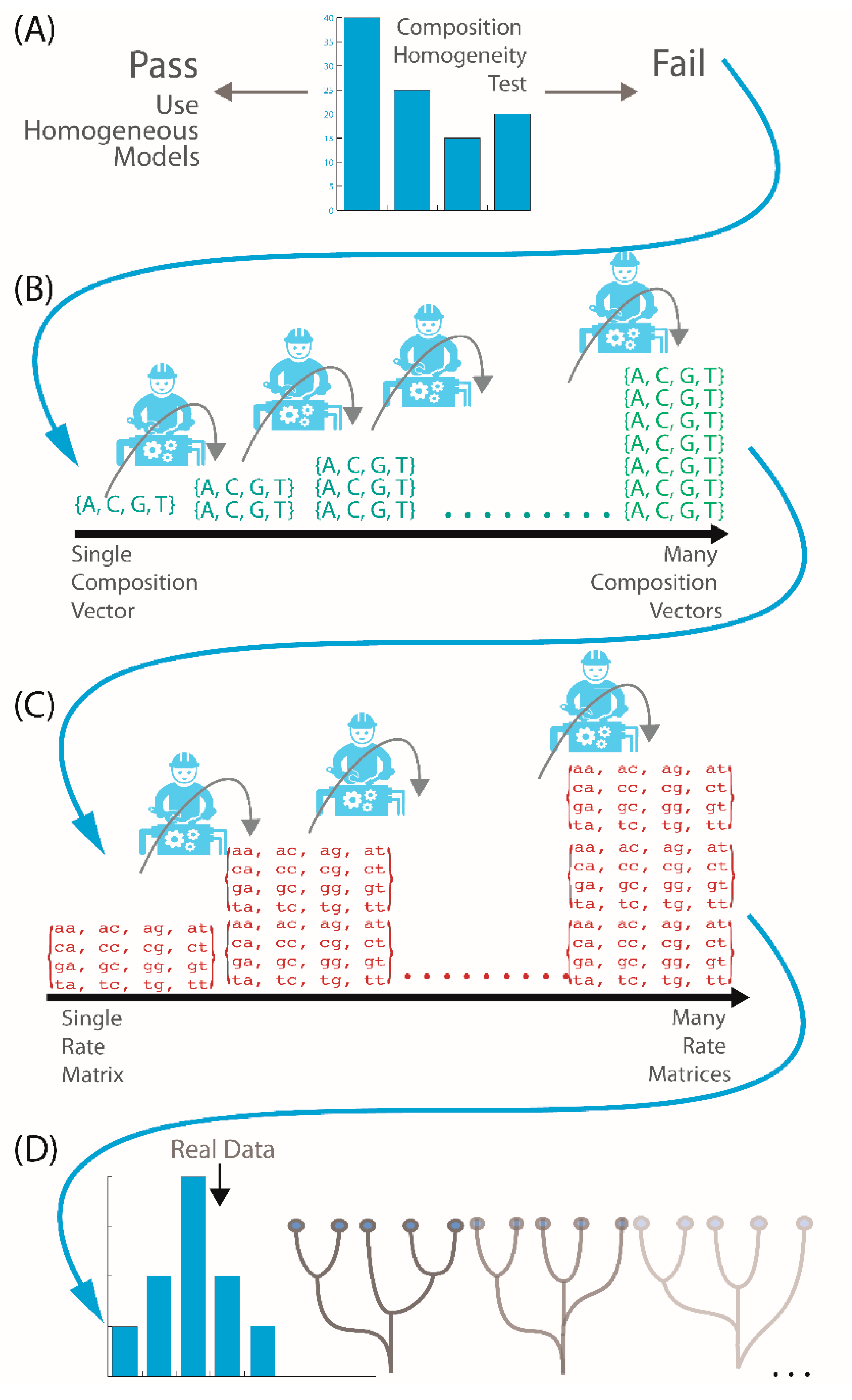
2.3. What If My Sequences Vary in Rates of Change across Their Length?

Not all sites within a gene evolve at the same rate, some are functionally constrained and are therefore highly conserved, whereas other sites such as the third position in a codon can be free to vary and have higher rates of change. Among site rate variation (ASRV) is therefore important when modeling evolution [2] and the gamma distribution has proven useful to this end [68,69]. The gamma distribution has a key shape parameter “α”, which gives it desirable flexible attributes and allows variation in substitution rates across sites. The gamma curve will change depending on α, for example α = 0.25 would have an “L-shaped” gamma curve and α = 10 would have a “bell-shaped” gamma curve. This flexibility is important, as some genes will have extreme ASRV and other will have a much smaller range. Using a discrete approximation of the gamma distribution, it is possible to define a number of rate categories to simplify the distribution, rather than integrating over the continuous curve. It has been shown [2] that four rate categories is sufficient for phylogenetic studies, where each uncertain site is analyzed in each rate category and a site rate that improves the model fit is estimated. The average likelihood across the four categories at each of these sites is used. In this way, the fast category will contribute most to the rapidly evolving sites and the slow category will contribute most to the slowly evolving sites [2]. This approach is commonly used to model rate heterogeneity [10]. The Invariance (+I) parameter is often used in models to account for sites in the dataset that do not change [70]. However, there is controversy around this parameter with some cautioning against using both +I and Gamma (+G) simultaneously [71] because the +G parameter accounts for invariance and therefore the +I and +G parameters affect each other’s estimations [72].

2.4. What If My Sequences Have Both Compositional Heterogeneity and Rate Heterogeneity?

Compositional heterogeneity using a node-discrete composition heterogeneity (NDCH) model and rate heterogeneity using a node-discrete rate heterogeneity (NDRH) model are implemented in P4 [10]. NDCH and NDRH can model heterogeneity between lineages. Other studies have implemented heterogeneity between lineages [73,74,75], and they have accomplished this using many parameters, meaning that over-parameterization can be an issue for reliable reconstruction and it does not scale well [76]. P4 is able to model heterogeneity using relatively few additional parameters [10]. It allows for multiple composition vectors and exchange rate matrices over the phylogeny and at any one time during the MCMC run each node is associated with one of the available composition vectors and exchange rate matrices. Therefore, each lineage can select the most appropriate model for itself (from a number of possible models). In most cases, this approach is more biologically realistic than homogeneous modeling [10]. It has been shown that the heterogeneous models in P4 are a better fit to mammal data than homogeneous models, and previous studies have produced erroneous topologies due to poor model fitting [7].

2.5. What If My Sequences Have Both Compositional and Rate Heterogeneity across Sites?

PhyloBayes uses a Bayesian framework for phylogenetic reconstruction [36] and it is capable of employing a model called CAT which is an infinite mixture model. As mentioned earlier this should not be confused with the CAT model of RAxML [35]. PhyloBayes is capable of modeling heterogeneity across sites; here the CAT model can account for site-specific amino acid or nucleotide parameters. Each column of the alignment is assigned to a profile that is most representative of the column. There are a number of profiles estimated from the data and each acts as a specific average of parameters. Therefore, instead of having one average set of parameters for the alignment (i.e., a homogeneous model) it is possible to have a number of specific averages that can model the different columns of the data (i.e., a heterogeneous model). In a way, this is a site-specific data partitioning without the need for prior knowledge. The CAT model has become particularly powerful with the release of PhyloBayes MPI [77] which facilitates the application of multiple processors to accelerate (up to a limit) the MCMC calculations [36,37,77].

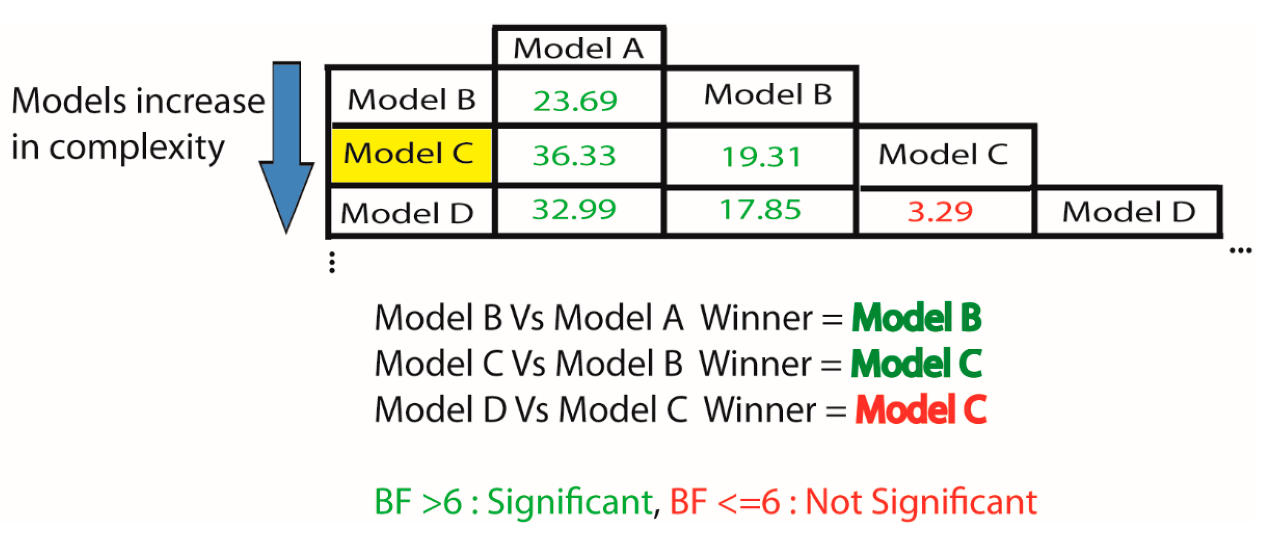
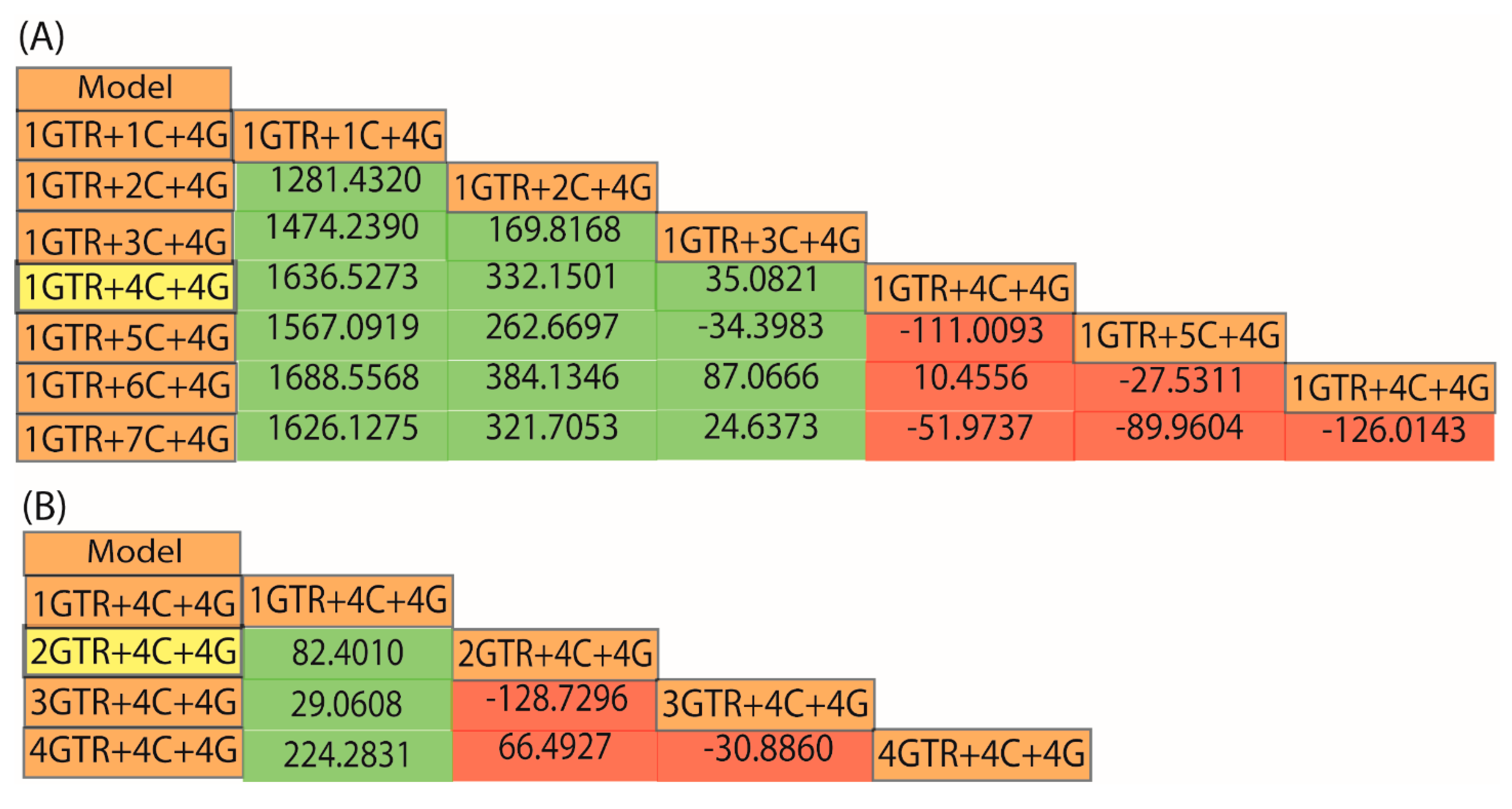
2.6. How Do I Select the Optimum Model for My Data?

Bayes Factor (BF) analysis is a Bayesian method that can be used to select between nested models (Figure 2) and this is particularly useful in P4 [10]. In P4 the user can vary the number of parameters of the core model, for example, the user can test a GTR model with two composition vectors and one rate matrix and compare this to a GTR model with three composition vectors and one rate matrix. There are many permutations of possible models with different numbers of composition vectors and rate matrices. BF analysis allows the user to find which one of the models fits the data best, always selecting for the model with the lowest number of parameters. Using Newton Raftery Equation (16) [78] within the P4 environment, the user can calculate the logarithm of the marginal likelihood and then compare the P4 models using the following test: 2[lnL(model B) − lnL(model A)] for each possible pairwise comparison of models. We compare the resulting value to the Kass and Raftery table [79]. If the value is greater than 6, then there is a strong indication that model B is a better fit to the data than model A. We then compare model C to model B in the same way and so on until we get a BF below 6. In which case, the model being tested is not a better fit to the data. There is no need to carry on at this point with the comparisons to the remaining models because we observe an increase parameterization that does not improve the fit (Figure 2) [10,79,80]. It is important that Bayes factor analysis and posterior predictive simulations described in step (vi) below are both used when one considers “does my model fit my data significantly?”

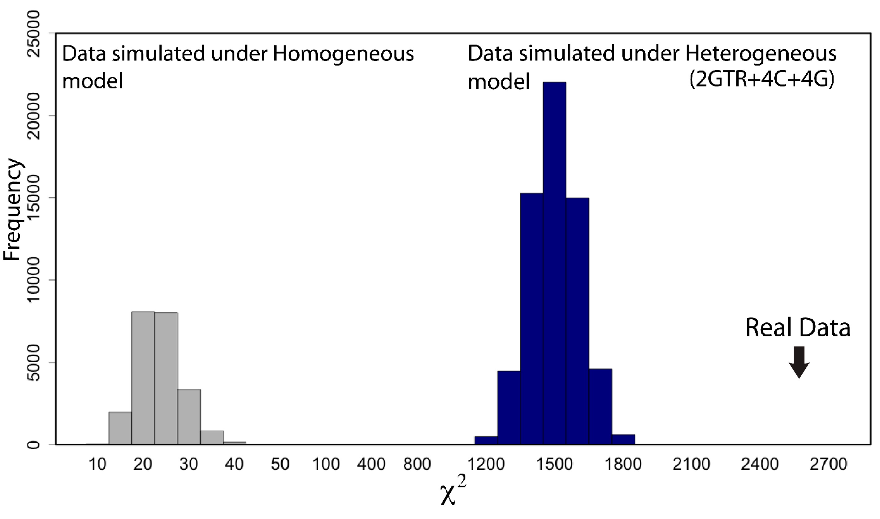
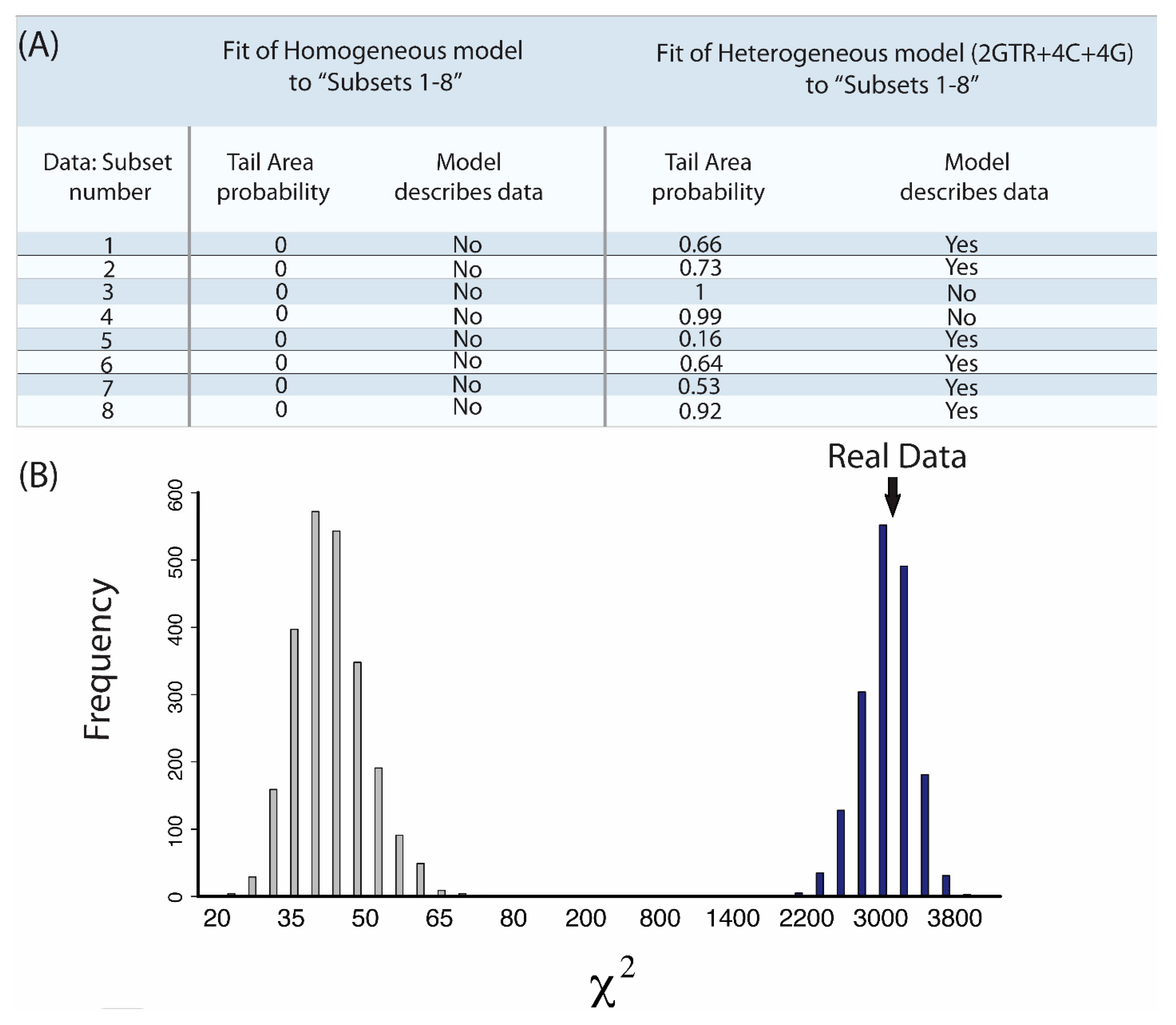
2.7. Does My Model Fit My Data?

Posterior predictive simulation (PPS) is a Bayesian model fit test that can be applied to both heterogeneous models and homogeneous models to give statistical support for how well a model describes a specific dataset [81]. Data is simulated under this model, and if the model describes the real data well, then our simulated data should be similar to the real data. Data is simulated based on the model used for the real data analysis and all the parameter estimations retrieved during the MCMC run. The simulated data can be compared to the real data through a single parameter—commonly the composition parameter is used for comparison. It is suggested that multinomial likelihood is used to test overall model fit and that the composition parameter is used to test how well this parameter is modeling the composition of the data [43]. Considering the resultant graphs from a PPS analysis, a model that fits well will plot the real test statistic close to the central mass of the histogram that is composed of the simulated test statistics (Figure 3 and Figure 4). From a statistical perspective, a tail area probability of 0.5 is optimal and indicates the model describes the data well [10]. In PhyloBayes the output of the PPS are given as a Z-score, where a Z-score >2 is an indication that the model does not fit the data [36].

Figure 2. Overview of a sample Bayes factor analysis. Models are denoted as A, B, C and D and parameters increase from A to D (i.e., Model A is the least parameterized model). They are compared in a pairwise manner as denoted by the lower triangular matrix. Each pairwise comparison results in a score (or Bayes Factor) by calculating 2[lnL(Model B) − lnL(Model A)]. Significance is based on the Kass and Raftery equation [79]. Cases where the Bayes Factor comparison yields a significant result are shown in green and models that do not significantly improve the fit to the data are given in red. Model C is selected as the “best-fit model” as an increase in parameters in Model D does not significantly improve the model fit. Therefore we do not continue to search more parameter rich models and we choose Model C (highlighted in yellow).

Figure 2. Overview of a sample Bayes factor analysis. Models are denoted as A, B, C and D and parameters increase from A to D (i.e., Model A is the least parameterized model). They are compared in a pairwise manner as denoted by the lower triangular matrix. Each pairwise comparison results in a score (or Bayes Factor) by calculating 2[lnL(Model B) − lnL(Model A)]. Significance is based on the Kass and Raftery equation [79]. Cases where the Bayes Factor comparison yields a significant result are shown in green and models that do not significantly improve the fit to the data are given in red. Model C is selected as the “best-fit model” as an increase in parameters in Model D does not significantly improve the model fit. Therefore we do not continue to search more parameter rich models and we choose Model C (highlighted in yellow).

Figure 3. Assessment of fit of the Homogeneous and Heterogeneous models for the RomiguierTopAT dataset. The leftmost histogram in grey shows the results of the posterior predictive simulation for RomiguierTopAT using the homogeneous model. The rightmost histogram in blue shows the improved posterior predictive simulation on modeling RomiguierTopAT with the heterogeneous model of best fit (i.e., 2GTR + 4C + 4G for RomiguierTopAT). In both simulations the X-axis represents the parameter of comparison taken from the simulations, and the Y-axis represents the frequency. The large black arrow indicates the value of test statistic (χ²) retrieved from the real data.

Figure 3. Assessment of fit of the Homogeneous and Heterogeneous models for the RomiguierTopAT dataset. The leftmost histogram in grey shows the results of the posterior predictive simulation for RomiguierTopAT using the homogeneous model. The rightmost histogram in blue shows the improved posterior predictive simulation on modeling RomiguierTopAT with the heterogeneous model of best fit (i.e., 2GTR + 4C + 4G for RomiguierTopAT). In both simulations the X-axis represents the parameter of comparison taken from the simulations, and the Y-axis represents the frequency. The large black arrow indicates the value of test statistic (χ²) retrieved from the real data.

Figure 4. Assessment of fit of Homogeneous and Heterogeneous models for “Subsets 1–8”. (A) Posterior predictive simulations for the “Subsets 1–8” are shown. The leftmost section of the table shows the results for the homogeneous model. The rightmost section of the table shows the improved tail area probability on modeling the data with heterogeneous models. Values closer to zero represent a poorer fit of the model to the data; (B) The results of the posterior predictive simulations for one subset (Subset 1) are shown in detail. Again the simulation for the homogeneous GTR model is shown in grey and the heterogeneous P4 model of best fit is shown in blue (i.e., 2GTR + 4C + 4G). In both simulations the X-axis represents the parameter of comparison taken from the simulations, and the Y-axis represents the frequency. The large black arrow indicates the value of test statistic (χ²) retrieved from the real data.

Figure 4. Assessment of fit of Homogeneous and Heterogeneous models for “Subsets 1–8”. (A) Posterior predictive simulations for the “Subsets 1–8” are shown. The leftmost section of the table shows the results for the homogeneous model. The rightmost section of the table shows the improved tail area probability on modeling the data with heterogeneous models. Values closer to zero represent a poorer fit of the model to the data; (B) The results of the posterior predictive simulations for one subset (Subset 1) are shown in detail. Again the simulation for the homogeneous GTR model is shown in grey and the heterogeneous P4 model of best fit is shown in blue (i.e., 2GTR + 4C + 4G). In both simulations the X-axis represents the parameter of comparison taken from the simulations, and the Y-axis represents the frequency. The large black arrow indicates the value of test statistic (χ²) retrieved from the real data.

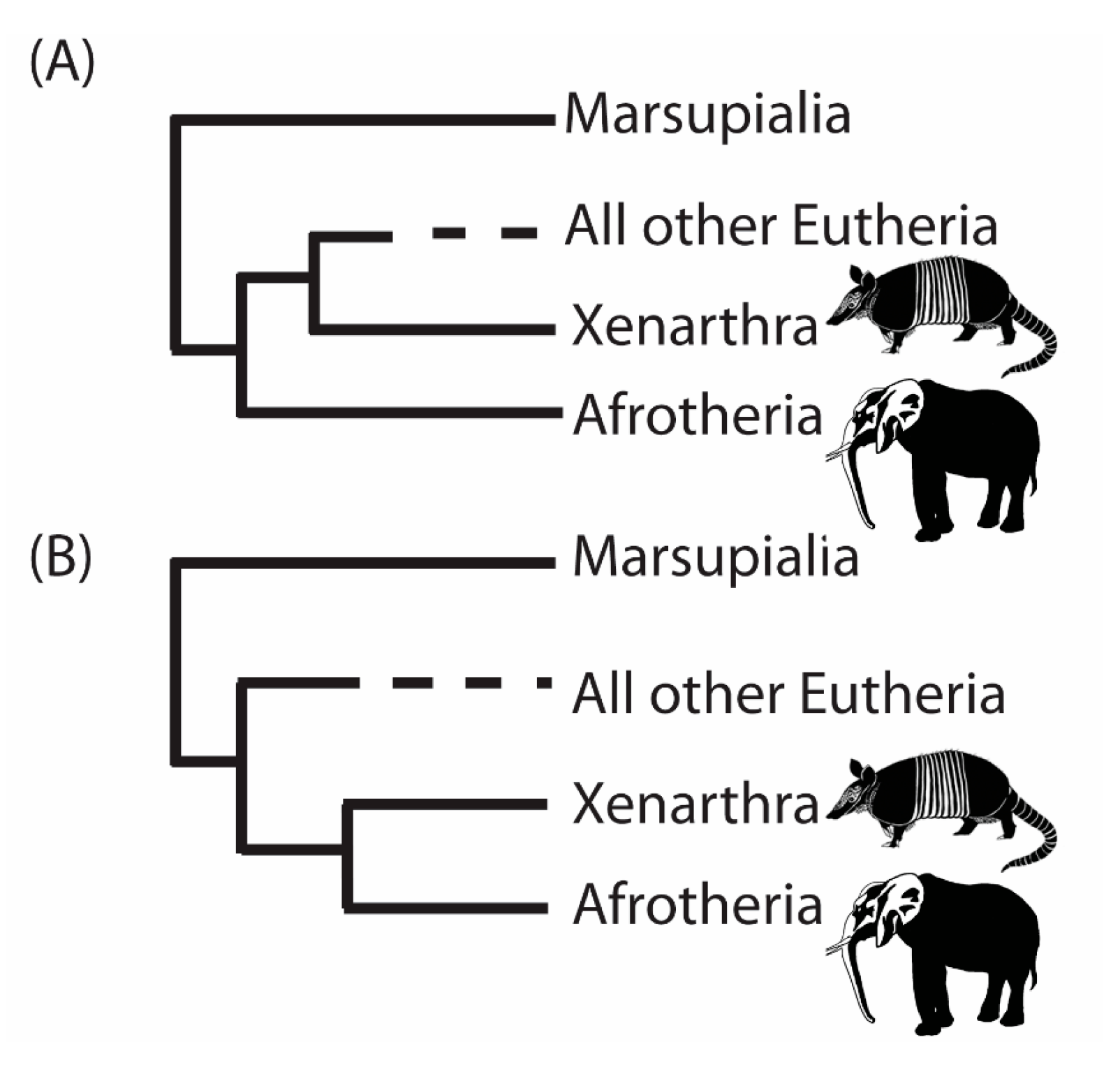
3. A Case Study from the Root of the Placental Mammal Tree

Placing the root of the placental mammal tree has been a controversial topic [82]. Many studies have concluded conflicting positions, sometimes even from the same pool of data [7,64,83,84,85]. In 2013, two molecular studies narrowed down the root of the placental mammal phylogeny to one of two possibilities: (i) an Afrotherian root which places mammals such as elephants as the earliest diverging placental mammal group [85]; and (ii) an Atlantogenata root, placing the common ancestor of the Xenarthra (e.g., armadillo) and Afrotheria as the earliest diverging placental mammal group [7].

In addition, it has been shown that previous studies of the position of the root of placental mammals lacked definitive resolution because of suboptimal models and datasets of low power [7]. It has been proposed that GC-rich genes lead to erroneous topologies (as GC is a proxy for recombination), and therefore that data partitioning should play a major role in the resolution of the mammal phylogeny. Evidently, the data and subsequent model used can greatly impact the result of the phylogenetic reconstruction. We demonstrate the application of the guidelines above to modeling the root of the placental mammal phylogeny. We propose that the conflicting positions for the root are due to model misspecification.

We set out to assess whether the models applied in the Romiguier et al. study were adequate for the data used [85]. In this study a set of mammal single gene orthologues were assembled from 39 mammal species and each of the 13,111 single gene families were categorized as GC-rich (>40% GC3 content) or AT-rich. The phylogenetic analysis of these datasets showed that GC-rich genes are most likely to support erroneous topologies and that AT-rich genes have a rate of error five times’ lower than that of GC-rich genes. The AT-rich genes supported an Afrotheria rooting, while the GC-rich genes supported an Atlantogenata rooting. The authors argued that the use of GC-rich genes contributes to conflict in the placement of the root of the placental mammal tree. The two datasets we use are named as per their original publication [85]:

(1)

“RomiguierTopAT”: This is a concatenated alignment using 100 of the most AT-rich genes. We wished to assess the impact of heterogeneous modeling on these data and on the support for the proposed Afrotheria hypothesis.

(2)

“Subsets 1–8”: Each of the eight subsets are a concatenated alignment using 25 genes chosen at random with varying GC-richness. We wished to assess whether heterogeneous models can adequately model the GC variation.

Following model selection analysis using ModelGenerator [15], the GTR model was selected. The results of the compositional homogeneity test showed that for the RomiguierTopAT of the 39 taxa, there were 12 that did not fit the homogeneous model. The RomiguierTopAT dataset therefore was compositionally heterogeneous but it was analyzed using a compositionally homogeneous model [85].

Using P4 [10] we tested to see if heterogeneous models describe the RomiguierTopAT dataset better than the original homogeneous models that were applied (Figure 3 and Figure 4). The standard procedure involved in the selection of a heterogeneous model in P4 is depicted in the schematic in Figure 1. When models had reached convergence, we completed the Bayes Factor (BF) analysis (Figure 5) to find the optimum number of composition vectors and then the optimum number of rate matrices for our model. Our optimum model for this dataset is annotated as 2GTR + 4C + 4G (2 GTR rate matrices, four composition vectors and four discrete gamma categories). The biggest improvement in BF score was 1281 and was for the comparison of the homogeneous model (1GTR + 1C + 4G) to the first heterogeneous model (1GTR + 2C + 4G). In addition to this, the number of composition vectors appears more important to model the data than the number of rate vectors (Figure 5). For each alignment we carried out the same procedure and each model tested was run with five independent runs until convergence was reached, with our expectation being topological agreement between independent runs. It is critical that the user is confident that convergence has been reached. We examined how the MCMC run progressed by examining the ASDOSS (average standard deviation of split supports) values of the checkpoints of the MCMC run. An ASDOSS <0.01 would suggest convergence has been reached. The likelihood values from the samples taken during the MCMC run were plotted to ensure that the likelihoods had reached a plateau [86]. The parameter acceptance rates are a rough indication of mixing and convergence.

Figure 5. Bayes factor analysis for RomiguierTopAT with heterogeneous models. The results depicted in (A) and (B) are for RomiguierTopAT, in both cases the BF result indicating the model of best fit is depicted in yellow. The overall model of best fit (for composition vectors and rate matrices) is 2GTR + 4C + 4G. (A) The lower triangular matrix of Bayes Factors used to find the optimum number of composition vectors for the model; (B) The lower triangular matrix of bayes factors used to find the optimum number of rate matrices. Combined they produce the best-fit model for the specific dataset. In both (A) and (B) significant improvements in model fit as judged by Kass and Raftery criteria [79] are shown in green and non-significant in red.

Figure 5. Bayes factor analysis for RomiguierTopAT with heterogeneous models. The results depicted in (A) and (B) are for RomiguierTopAT, in both cases the BF result indicating the model of best fit is depicted in yellow. The overall model of best fit (for composition vectors and rate matrices) is 2GTR + 4C + 4G. (A) The lower triangular matrix of Bayes Factors used to find the optimum number of composition vectors for the model; (B) The lower triangular matrix of bayes factors used to find the optimum number of rate matrices. Combined they produce the best-fit model for the specific dataset. In both (A) and (B) significant improvements in model fit as judged by Kass and Raftery criteria [79] are shown in green and non-significant in red.

A consensus tree was made from the MCMC run for the RomiguierTopAT dataset under the 2GTR + 4C + 4G model. The topology supported the Afrotheria position of the root (Figure 6A). However, posterior predictive simulations (PPS) reveal a poor tail area probability of 0.00, showing that this model does not adequately describe the data and that the resultant topology is not robust. We went on to assess whether any of the 24 P4 models tested had a significant tail area probability for RomiguierTopAT. Surprisingly, none of the models had a significant tail area probability; in fact, all models we tested had a tail area probability of 0.00, suggesting that P4 cannot model this data adequately with the models available. However, the simulated dataset produced using the heterogeneous P4 models are a better fit to the real data than the homogeneous model (Figure 3). As such, the topology is not significantly supported. This is unusual as P4 is generally capable of showing some model fit. The RomiguierTopAT dataset seems to be very difficult to model adequately, perhaps this is due to a combination of a high level of heterogeneity across sites and between lineages. But it is clear from these analyses that homogeneous modeling is too simplistic and not realistic for this dataset. Morgan et al. (2013) showed significant support for the Atlantogenata root using both P4 and PhyloBayes [36], but more importantly, the models were shown to adequately describe the data [7]. The analysis of Subsets 1–8 in P4 showed some model fit for all these subsets and in all cases of Subsets1–8 the heterogeneous model was a better fitting model than a homogeneous. In most cases (6/8 of the subsets) the heterogeneous model significantly fits the data (Figure 4). These results for Subsets 1–8 illustrate that heterogeneous models are capable of adequately modeling complex data and are more appropriate than homogeneous models for the data.

Figure 6. Analysis of the position of the mammal root using three different methods. (A) Afrotheria position retrieved using RomiguierTopAT alignment and the GTR model in RAxML (result = Afrotheria position for the root), and also using the optimum available P4 model; and (B) Atlantogenata position retrieved using the 39 taxa mammal dataset from Morgan et al. [7] with the CAT-GTR model in PhyloBayes.

Figure 6. Analysis of the position of the mammal root using three different methods. (A) Afrotheria position retrieved using RomiguierTopAT alignment and the GTR model in RAxML (result = Afrotheria position for the root), and also using the optimum available P4 model; and (B) Atlantogenata position retrieved using the 39 taxa mammal dataset from Morgan et al. [7] with the CAT-GTR model in PhyloBayes.

In general, P4 is a powerful approach for phylogeny reconstruction as it contains many sophisticated tools for phylogenetic analysis and assessment of models, including methods to test the fit of the model to the data in the form of posterior predictive simulations. Through our analysis of the RomiguierTopAT data using P4 it was clear that a heterogeneous approach was needed, therefore we applied the PhyloBayes heterogeneous model CAT [36] and P4 tests of alternative heterogeneous models. The results of the PhyloBayes analysis for the placement of the position of the mammal root have been described previously by Morgan et al. (2013) for a dataset derived from the same pool of data as the RomiguierTopAT dataset [7]. Here, the CAT-GTR model in PhyloBayes [36] was also applied to the RomiguierTopAT alignment and strong support for the Atlantogenata position for the root was subsequently retrieved. Importantly, Morgan et al. (2013) showed that for their dataset [6] the CAT-GTR model adequately described and fit the data and that homogeneous models did not. Our analysis using P4 illustrates that a homogeneous modeling approach is not suitable for the RomiguierTopAT data. [Note: In a PhyloBayes [36] analysis the number of biochemical categories is optimized during the tree search, therefore if the GTR model (which is nested within the CAT-GTR model) is a better fit to the data than the CAT-GTR model, then the CAT-GTR model will reduce to the simpler GTR model, thus relinquishing the need to independently test the GTR model on the data.]

4. Conclusions

Combining the sophisticated modeling approach in P4 [10] as described in Morgan et al. (2013) [7] and the data partitioning method of Romiguier, Ranwez et al. (2013) [85], we show that homogeneous models do not describe the RomiguierTopAT data adequately and therefore any topology resulting from that model is not significant. While software packages such as RAxML [35] can be incredibly powerful and fast, they are not always appropriate for specific datasets. The results for the datasets “Subsets 1–8” indicate that modeling heterogeneity across the phylogeny will not always work for a specific dataset. In this case, we searched for the optimum heterogeneous GTR model and still failed to adequately model the data. This serves to highlight the importance of checking the adequacy of the model for each specific dataset. One cannot assume that any heterogeneous model is adequate. One can only trust the phylogeny produced with a model that adequately and statistically significantly models that data. However, the question the user needs to ask is “does this model adequately describe my data” and if the answer is no then the resultant topology is not reliable. The key is to resist making assumptions of the data and instead let the data dictate the approach and the model. As genome-scale phylogenies become commonplace and as consilience across data types rapidly takes hold as best practice, the importance of developing methods that can efficiently and adequately model data is paramount. We have outlined a step-by-step procedure for reconstructing a robust phylogeny using appropriate current models, but the onus is very much on the user to understand the methods they apply, and to fully and critically assess the limitations of their data and their approach.

References

1. Posada, D. Selecting Models of Evolution. In The Phylogenetic Handbook: A Practical Approach to DNA and Protein Phylogeny; Cambridge University Press: Cambridge, UK, 2003. [Google Scholar]
2. Yang, Z. Among-site rate variation and its impact on phylogenetic analyses. Trends Ecol. Evol. 1996, 11, 367–372. [Google Scholar] [CrossRef] [PubMed]
3. Gouy, M.; Li, W.-H. Phylogenetic analysis based on rRNA sequences supports the archaebacterial rather than the eocyte tree. Nature 1989, 339, 145–147. [Google Scholar] [CrossRef] [PubMed]
4. Tourasse, N.J.; Gouy, M. Accounting for evolutionary rate variation among sequence sites consistently changes universal phylogenies deduced from rRNA and protein-coding genes. Mol. Phylogenet. Evol. 1999, 13, 159–168. [Google Scholar] [CrossRef] [PubMed]
5. Li, W.-H.; Tanimura, M.; Sharp, P.M. An evaluation of the molecular clock hypothesis using mammalian DNA sequences. J. Mol. Evol. 1987, 25, 330–342. [Google Scholar] [CrossRef] [PubMed]
6. Romiguier, J.; Ranwez, V.; Douzery, E.J.P.; Galtier, N. Contrasting GC-content dynamics across 33 mammalian genomes: Relationship with life-history traits and chromosome sizes. Genome Res. 2010, 20, 1001–1009. [Google Scholar] [CrossRef] [PubMed]
7. Morgan, C.C.; Foster, P.G.; Webb, A.E.; Pisani, D.; McInerney, J.O.; O’Connell, M.J. Heterogeneous models place the root of the placental mammal phylogeny. Mol. Biol. Evol. 2013, 30, 2145–2156. [Google Scholar] [CrossRef] [PubMed]
8. Galtier, N.; Duret, L. Adaptation or biased gene conversion? Extending the null hypothesis of molecular evolution. Trends Genet. 2007, 23, 273–277. [Google Scholar]
9. Galtier, N.; Piganeau, G.; Mouchiroud, D.; Duret, L. GC-content evolution in mammalian genomes: The biased gene conversion hypothesis. Genetics 2001, 159, 907–911. [Google Scholar] [PubMed]
10. Foster, P.G. Modeling compositional heterogeneity. Syst. Biol. 2004, 53, 485–495. [Google Scholar] [CrossRef] [PubMed]
11. Olmstead, R.G. Molecular Systematics, 2nd ed.; Hillis, D.M., Moritz, C., Mable, B.K., Eds.; Sinauer Associates: Sunderland, MA, USA, 1996. [Google Scholar]
12. Abascal, F.; Zardoya, R.; Posada, D. ProtTest: Selection of best-fit models of protein evolution. Bioinformatics 2005, 21, 2104–2105. [Google Scholar] [CrossRef] [PubMed]
13. Posada, D.; Crandall, K.A. Modeltest: Testing the model of DNA substitution. Bioinformatics 1998, 14, 817–818. [Google Scholar] [CrossRef] [PubMed]
14. Nylander, J.A.A. MrModeltest v2. Program Distributed by the Author; Evolutionary Biology Centre, Uppsala University: Uppsala, Sweden, 2004. [Google Scholar]
15. Keane, T.M.; Naughton, T.J.; McInerney, J.O. ModelGenerator: Amino Acid and Nucleotide Substitution Model Selection; National University of Ireland: Maynooth, Ireland, 2004. [Google Scholar]
16. Dayhoff, M.O.; Schwartz, R.M. A Model of Evolutionary Change in Proteins. In Atlas of Protein Sequence and Structure; National Biomedical Research Foundation: Washington, DC, USA, 1978. [Google Scholar]
17. Liò, P.; Goldman, N. Models of molecular evolution and phylogeny. Genome Res. 1998, 8, 1233–1244. [Google Scholar] [PubMed]
18. Phillips, M.J.; Penny, D. The root of the mammalian tree inferred from whole mitochondrial genomes. Mol. Phylogenet. Evol. 2003, 28, 171–185. [Google Scholar] [CrossRef] [PubMed]
19. Ishikawa, S.A.; Inagaki, Y.; Hashimoto, T. RY-coding and non-homogeneous models can ameliorate the maximum-likelihood inferences from nucleotide sequence data with parallel compositional heterogeneity. Evolut. Bioinform. Online 2012, 8, 357. [Google Scholar] [CrossRef]
20. Jukes, T.H.; Cantor, C.R. Evolution of protein molecules. Mamm. Protein Metab. 1969, 3, 121–132. [Google Scholar]
21. Felsenstein, J. Evolutionary trees from DNA sequences: A maximum likelihood approach. J. Mol. Evol. 1981, 17, 368–376. [Google Scholar] [CrossRef] [PubMed]
22. Felsenstein, J.; Churchill, G.A. A Hidden Markov Model approach to variation among sites in rate of evolution. Mol. Biol. Evol. 1996, 13, 93–104. [Google Scholar] [CrossRef] [PubMed]
23. Tavaré, S. Some probabilistic and statistical problems in the analysis of DNA sequences. Lect. Math. Life Sci. 1986, 17, 57–86. [Google Scholar]
24. Jones, D.T.; Taylor, W.R.; Thornton, J.M. A mutation data matrix for transmembrane proteins. FEBS Lett. 1994, 339, 269–275. [Google Scholar] [CrossRef] [PubMed]
25. Whelan, S.; Goldman, N. A general empirical model of protein evolution derived from multiple protein families using a maximum-likelihood approach. Mol. Biol. Evol. 2001, 18, 691–699. [Google Scholar] [CrossRef] [PubMed]
26. Abascal, F.; Posada, D.; Zardoya, R. MtArt: A new model of amino acid replacement for Arthropoda. Mol. Biol. Evol. 2007, 24, 1–5. [Google Scholar] [CrossRef] [PubMed]
27. Adachi, J.; Waddell, P.J.; Martin, W.; Hasegawa, M. Plastid genome phylogeny and a model of amino acid substitution for proteins encoded by chloroplast DNA. J. Mol. Evol. 2000, 50, 348–358. [Google Scholar] [PubMed]
28. Cao, Y.; Adachi, J.; Janke, A.; Pääbo, S.; Hasegawa, M. Phylogenetic relationships among eutherian orders estimated from inferred sequences of mitochondrial proteins: Instability of a tree based on a single gene. J. Mol. Evol. 1994, 39, 519–527. [Google Scholar] [CrossRef] [PubMed]
29. Nickle, D.C.; Heath, L.; Jensen, M.A.; Gilbert, P.B.; Mullins, J.I.; Kosakovsky Pond, S.L. HIV-specific probabilistic models of protein evolution. PLoS ONE 2007, 2, e503. [Google Scholar] [CrossRef] [PubMed]
30. Dimmic, M.W.; Rest, J.S.; Mindell, D.P.; Goldstein, R.A. rtREV: An amino acid substitution matrix for inference of retrovirus and reverse transcriptase phylogeny. J. Mol. Evol. 2002, 55, 65–73. [Google Scholar] [CrossRef] [PubMed]
31. Henikoff, S.; Henikoff, J.G. Amino acid substitution matrices from protein blocks. Proc. Natl. Acad. Sci. USA 1992, 89, 10915–10919. [Google Scholar] [CrossRef] [PubMed]
32. Le, S.Q.; Gascuel, O. An improved general amino acid replacement matrix. Mol. Biol. Evol. 2008, 25, 1307–1320. [Google Scholar] [CrossRef] [PubMed]
33. Müller, T.; Vingron, M. Modeling amino acid replacement. J. Comput. Biol. 2000, 7, 761–776. [Google Scholar] [CrossRef] [PubMed]
34. Stamatakis, A. Phylogenetic models of rate heterogeneity: A high performance computing perspective. In Proceedings of the 20th International Parallel and Distributed Processing Symposium (IPDPS 2006), Rhodes Island, Greece, 25–29 April 2006.
35. Stamatakis, A. RAxML-VI-HPC: Maximum likelihood-based phylogenetic analyses with thousands of taxa and mixed models. Bioinformatics 2006, 22, 2688–2690. [Google Scholar] [CrossRef] [PubMed]
36. Lartillot, N.; Lepage, T.; Blanquart, S. PhyloBayes 3: A Bayesian software package for phylogenetic reconstruction and molecular dating. Bioinformatics 2009, 25, 2286–2288. [Google Scholar] [CrossRef] [PubMed]
37. Lartillot, N.; Philippe, H. A Bayesian mixture model for across-site heterogeneities in the amino-acid replacement process. Mol. Biol. Evol. 2004, 21, 1095–1109. [Google Scholar] [CrossRef] [PubMed]
38. Douady, C.J.; Delsuc, F.; Boucher, Y.; Doolittle, W.F.; Douzery, E.J.P. Comparison of Bayesian and maximum likelihood bootstrap measures of phylogenetic reliability. Mol. Biol. Evol. 2003, 20, 248–254. [Google Scholar] [CrossRef] [PubMed]
39. Huelsenbeck, J.P.; Crandall, K.A. Phylogeny estimation and hypothesis testing using maximum likelihood. Annu. Rev. Ecol. Syst. 1997, 28, 437–466. [Google Scholar] [CrossRef]
40. Felsenstein, J. Cases in which parsimony or compatibility methods will be positively misleading. Syst. Biol. 1978, 27, 401–410. [Google Scholar] [CrossRef]
41. Brown, J.K. Bootstrap hypothesis tests for evolutionary trees and other dendrograms. Proc. Natl. Acad. Sci. USA 1994, 91, 12293–12297. [Google Scholar] [CrossRef] [PubMed]
42. Shafer, G. A Mathematical Theory of Evidence; Princeton University Press: Princeton, NJ, USA, 1976; Volume 1. [Google Scholar]
43. Huelsenbeck, J.P.; Ronquist, F.; Nielsen, R.; Bollback, J.P. Bayesian inference of phylogeny and its impact on evolutionary biology. Science 2001, 294, 2310–2314. [Google Scholar] [CrossRef] [PubMed]
44. Hastings, W.K. Monte Carlo sampling methods using Markov chains and their applications. Biometrika 1970, 57, 97–109. [Google Scholar] [CrossRef]
45. Metropolis, N.; Rosenbluth, A.W.; Rosenbluth, M.N.; Teller, A.H.; Teller, E. Equation of state calculations by fast computing machines. J. Chem. Phys. 1953, 21, 1087–1092. [Google Scholar] [CrossRef]
46. Altekar, G.; Dwarkadas, S.; Huelsenbeck, J.P.; Ronquist, F. Parallel metropolis coupled Markov chain Monte Carlo for Bayesian phylogenetic inference. Bioinformatics 2004, 20, 407–415. [Google Scholar] [CrossRef] [PubMed]
47. Gatesy, J.; Springer, M.S. Phylogenetic analysis at deep timescales: Unreliable gene trees, bypassed hidden support, and the coalescence/concatalescence conundrum. Mol. Phylogenet. Evol. 2014, 80, 231–266. [Google Scholar] [CrossRef] [PubMed]
48. Song, S.; Liu, L.; Edwards, S.V.; Wu, S. Resolving conflict in eutherian mammal phylogeny using phylogenomics and the multispecies coalescent model. Proc. Natl. Acad. Sci. USA 2012, 109, 14942–14947. [Google Scholar] [CrossRef] [PubMed]
49. Lanfear, R.; Calcott, B.; Ho, S.Y.W.; Guindon, S. PartitionFinder: Combined selection of partitioning schemes and substitution models for phylogenetic analyses. Mol. Biol. Evol. 2012, 29, 1695–1701. [Google Scholar] [CrossRef] [PubMed]
50. Cummins, C.A.; McInerney, J.O. A method for inferring the rate of evolution of homologous characters that can potentially improve phylogenetic inference, resolve deep divergence and correct systematic biases. Syst. Biol. 2011, 60, 833–844. [Google Scholar] [CrossRef] [PubMed]
51. Frandsen, P.B.; Calcott, B.; Mayer, C.; Lanfear, R. Automatic selection of partitioning schemes for phylogenetic analyses using iterative k-means clustering of site rates. BMC Evolut. Biol. 2015, 15, 13. [Google Scholar] [CrossRef]
52. Lanfear, R.; Calcott, B.; Kainer, D.; Mayer, C.; Stamatakis, A. Selecting optimal partitioning schemes for phylogenomic datasets. BMC Evolut. Biol. 2014, 14, 82. [Google Scholar] [CrossRef]
53. Capella-Gutierrez, S.; Silla-Martinez, J.M.; Gabaldn, T. TrimAl: A tool for automated alignment trimming in large-scale phylogenetic analyses. Bioinformatics 2009, 25, 1972–1973. [Google Scholar] [CrossRef] [PubMed]
54. Morrison, D.A.; Ellis, J.T. Effects of nucleotide sequence alignment on phylogeny estimation: A case study of 18S rDNAs of Apicomplexa. Mol. Biol. Evol. 1997, 14, 428–441. [Google Scholar] [CrossRef] [PubMed]
55. Muller, J.; Creevey, C.J.; Thompson, J.D.; Arendt, D.; Bork, P. AQUA: Automated quality improvement for multiple sequence alignments. Bioinformatics 2010, 26, 263–265. [Google Scholar] [CrossRef] [PubMed]
56. Notredame, C. Recent evolutions of multiple sequence alignment algorithms. PLoS Comput. Biol. 2007, 3, e123. [Google Scholar] [CrossRef] [PubMed]
57. Phillips, A.; Janies, D.; Wheeler, W. Multiple sequence alignment in phylogenetic analysis. Mol. Phylogenet. Evol. 2000, 16, 317–330. [Google Scholar] [CrossRef] [PubMed]
58. Thompson, J.D.; Thierry, J.C.; Poch, O. RASCAL: Rapid scanning and correction of multiple sequence alignments. Bioinformatics 2003, 19, 1155–1161. [Google Scholar] [CrossRef] [PubMed]
59. Blackburne, B.P.; Whelan, S. Measuring the distance between multiple sequence alignments. Bioinformatics 2012, 28, 495–502. [Google Scholar] [CrossRef] [PubMed]
60. Gibson, A.; Gowri-Shankar, V.; Higgs, P.G.; Rattray, M. A comprehensive analysis of mammalian mitochondrial genome base composition and improved phylogenetic methods. Mol. Biol. Evol. 2005, 22, 251–264. [Google Scholar] [CrossRef] [PubMed]
61. Kjer, K.M.; Honeycutt, R.L. Site specific rates of mitochondrial genomes and the phylogeny of eutheria. BMC Evolut. Biol. 2007, 7, 8. [Google Scholar] [CrossRef]
62. Reyes, A.; Gissi, C.; Catzeflis, F.; Nevo, E.; Pesole, G.; Saccone, C. Congruent mammalian trees from mitochondrial and nuclear genes using Bayesian methods. Mol. Biol. Evol. 2004, 21, 397–403. [Google Scholar] [CrossRef] [PubMed]
63. Arnason, U.; Janke, A. Mitogenomic analyses of eutherian relationships. Cytogenet. Genome Res. 2002, 96, 20–32. [Google Scholar] [CrossRef] [PubMed]
64. Springer, M.S.; Stanhope, M.J.; Madsen, O.; de Jong, W.W. Molecules consolidate the placental mammal tree. Trends Ecol. Evol. 2004, 19, 430–438. [Google Scholar] [CrossRef] [PubMed]
65. Morgan, C.C.; Creevey, C.J.; O’Connell, M.J. Mitochondrial data are not suitable for resolving placental mammal phylogeny. Mamm. Genome 2014, 25, 636–647. [Google Scholar] [CrossRef] [PubMed]
66. Misof, B.; Liu, S.; Meusemann, K.; Peters, R.S.; Donath, A.; Mayer, C.; Frandsen, P.B.; Ware, J.; Flouri, T.; Beutel, R.G. Phylogenomics resolves the timing and pattern of insect evolution. Science 2014, 346, 763–767. [Google Scholar] [CrossRef] [PubMed]
67. Brown, T.A. Molecular Phylogenetics. In Genomes, 2nd ed.; Garland Science: New York, NY, USA, 2002. [Google Scholar]
68. Hasegawa, M. Phylogeny and molecular evolution in primates. Jpn. J. Genet. 1990, 65, 243–266. [Google Scholar] [CrossRef] [PubMed]
69. Li, W.-H.; Gouy, M.; Sharp, P.M.; O’Huigin, C.; Yang, Y.-W. Molecular phylogeny of Rodentia, Lagomorpha, Primates, Artiodactyla, and Carnivora and molecular clocks. Proc. Natl. Acad. Sci. USA 1990, 87, 6703–6707. [Google Scholar] [CrossRef] [PubMed]
70. Reeves, J.H. Heterogeneity in the substitution process of amino acid sites of proteins coded for by mitochondrial DNA. J. Mol. Evol. 1992, 35, 17–31. [Google Scholar] [CrossRef] [PubMed]
71. Yang, Z. Computational Molecular Evolution; Oxford University Press: Oxford, UK, 2006. [Google Scholar]
72. Mayrose, I.; Friedman, N.; Pupko, T. A Gamma mixture model better accounts for among site rate heterogeneity. Bioinformatics 2005, 21, ii151–ii158. [Google Scholar] [CrossRef] [PubMed]
73. Galtier, N.; Gouy, M. Inferring pattern and process: Maximum-likelihood implementation of a nonhomogeneous model of DNA sequence evolution for phylogenetic analysis. Mol. Biol. Evol. 1998, 15, 871–879. [Google Scholar] [CrossRef] [PubMed]
74. Galtier, N.; Tourasse, N.; Gouy, M. A nonhyperthermophilic common ancestor to extant life forms. Science 1999, 283, 220–221. [Google Scholar] [CrossRef] [PubMed]
75. Yang, Z.; Roberts, D. On the use of nucleic acid sequences to infer early branchings in the tree of life. Mol. Biol. Evol. 1995, 12, 451–458. [Google Scholar] [PubMed]
76. Rannala, B. Identifiability of parameters in MCMC Bayesian inference of phylogeny. Syst. Biol. 2002, 51, 754–760. [Google Scholar] [CrossRef] [PubMed]
77. Lartillot, N.; Rodrigue, N.; Stubbs, D.; Richer, J. PhyloBayes MPI. Phylogenetic reconstruction with infinite mixtures of profiles in a parallel environment. Syst. Biol. 2013, 62, 611–615. [Google Scholar]
78. Newton, M.A.; Raftery, A.E. Approximate Bayesian inference with the weighted likelihood bootstrap. J. R. Statist. Soc. Ser. B Methodol. 1994, 58, 3–48. [Google Scholar]
79. Kass, R.E.; Raftery, A.E. Bayes factors. J. Am. Stat. Assoc. 1995, 90, 773–795. [Google Scholar] [CrossRef]
80. Lopes, H.F.; West, M. Bayesian model assessment in factor analysis. Stat. Sin. 2004, 14, 41–68. [Google Scholar]
81. Gelman, A.; Carlin, J.B.; Stern, H.S.; Dunson, D.B.; Vehtari, A.; Rubin, D.B. Bayesian Data Analysis; CRC Press: Boca Raton, FL, USA, 2013. [Google Scholar]
82. Teeling, E.C.; Hedges, S.B. Making the impossible possible: Rooting the tree of placental mammals. Mol. Biol. Evol. 2013, 30, 1999–2000. [Google Scholar] [CrossRef] [PubMed]
83. Murphy, W.J.; Pringle, T.H.; Crider, T.A.; Springer, M.S.; Miller, W. Using genomic data to unravel the root of the placental mammal phylogeny. Genome Res. 2007, 17, 413–421. [Google Scholar] [CrossRef] [PubMed]
84. Prasad, A.B.; Allard, M.W.; Green, E.D. Confirming the phylogeny of mammals by use of large comparative sequence data sets. Mol. Biol. Evol. 2008, 25, 1795–1808. [Google Scholar] [CrossRef] [PubMed]
85. Romiguier, J.; Ranwez, V.; Delsuc, F.; Galtier, N.; Douzery, E.J.P. Less is more in mammalian phylogenomics: AT-rich genes minimize tree conflicts and unravel the root of placental mammals. Mol. Biol. Evol. 2013, 30, 2134–2144. [Google Scholar] [CrossRef] [PubMed]
86. Nylander, J.A.A.; Wilgenbusch, J.C.; Warren, D.L.; Swofford, D.L. AWTY (are we there yet?): A system for graphical exploration of MCMC convergence in Bayesian phylogenetics. Bioinformatics 2008, 24, 581–583. [Google Scholar]