Coupling of Petri Net Models of the Mycobacterial Infection Process and Innate Immune Response

Abstract

Computational and mathematical modeling is important in support of a better understanding of complex behavior in biology. For the investigation of biological systems, researchers have used computers to construct, verify, and validate models that describe the mechanisms behind biological processes in multi-scale representations. In this paper we combine Petri net models that represent the mycobacterial infection process and innate immune response at various levels of organization, from molecular interaction to granuloma dissemination. In addition to the conventional graphical representation of the Petri net, the outcome of the model is projected onto a 3D model representing the zebrafish embryo. In this manner we provide a visualization of the process in a simulation framework that portrays the infection in the living system.

1. Introduction

The understanding of the highly complex world of immunology is a major challenge for scientists in the fields of biology, medicine, and pharmacology. For the description of biological phenomena related to the immune system, the modeling, simulation, and analysis of the immune system are considered important practices and can contribute to improved diagnostics and optimized immune treatments. For that purpose, mathematical and computational methodologies have been utilized to create models that represent biological behavior. These models can support explanations of the interaction mechanisms between pathogenic agents and the defense mechanism in intuitive and yet analyzable terms.

In the context of our research, a mathematical model is a formal model describing by means of equations relationships between quantities and how quantities change over time. Computational models such as agent-based models (ABMs) describe dependencies between activities of components of a system. Combinations of the two approaches have been used to describe, simulate, and analyze the networks and interactions in the immune system [1,2,3,4,5]. Pappalardo et al. provided an extensive study on vaccine administration and immune response to cancer in mice by implementing and simulating models using ABMs and cellular automata [6,7,8]. Gammack et al. [9] provided a mathematical model based on Ordinary Differential Equations (ODEs) to investigate the early and initial immune response to mycobacterial infection (Mtb) in mice. This work has inspired Segovia-Juarez et al. [10] to implement the ODEs that regulate the interaction between host and pathogen using an ABM approach. Warrender et al. [11] use the CyCell simulator tool to simulate the interactions in early mycobacterial infection.

The different scales of the models can be an obstacle to modeling the infection process and the immune response. For biologists, it is intuitive to establish a process that involves cells, molecules, and/or organs. It is, however, not trivial to identify the line of information retrieval that connects/switches from one level to the next [12]. A multi-scale approach has been used to connect interactions at molecular, cellular, and tissue level as well as the modeling of the dynamics from a spatial and temporal perspective. Multi-scale models, including how to connect different individual levels, have been extensively explored, e.g., [12,13,14,15]. In the study of the mycobacterial infection process and immune response, establishing an adequate method to account for multi-scale processes is still a challenge. In mathematical models, like those based on differential equations, the interactions are described in rules and equations, whereas computational models are embedded in programming code with which one cannot interact in a straightforward manner; neither can one directly understand its structure.

Thus, a graphical representation of the interactions and influences among various components that involve the bacteria and host immune cells, i.e., molecules and proteins, that also captures the dynamics of the system would be very useful. The Petri net formalism (PN) represents a well-established technique in which a graphical representation is combined with a mathematical basis for modeling distributed concurrent systems [16,17]. Petri nets are successfully used to model biological behavior [18,19]. Heiner et al. [20] propose a methodology of incremental modeling using Petri nets to develop and analyze a qualitative model of the apoptotic pathway. Albergante et al. [21] have developed a Petri net model that simulates the formation of hepatic granuloma for Leishimania donavani infection in mice.

In previous work [22], we have developed a qualitative Petri net model of the mycobacterial infection process and the subsequent innate immune response. We organized our model at the level of cell dynamics, and it is characterized by steps involved in the Mycobacterium marinum infection and granuloma formation in zebrafish. Subsequently, we used Petri nets to model the interactions between the bacteria and the host immune cell in a multi-scale approach [23], connecting important pathways involved in the host-pathogen interactions that are acting over different scales (molecular, intracellular, and intercellular) during the innate immune response.

In this paper, we extend our two previous models by combining them in a hierarchical fashion, so as to jointly represent the mycobacterial infection process and innate immune response. The qualitative model captures the relationship between the pathogen and the host immune cells, i.e., the bacteria and the macrophages, from the perspective of cell dynamics down to interactions at intercellular, intracellular, and molecular level. The hierarchical model provides a visualization of the infection process from the moment the bacteria enter the host: the migration, proliferation, granuloma formation, and dissemination. Moreover, it models the signaling pathways that a macrophage employs to terminate the infection and the way the bacterium exploits those pathways to enhance its intracellular survival persistence. In this paper we introduce an additional visualization, which renders the infection process as modeled and simulated with the qualitative Petri nets on a 3D mesh model of the zebrafish. It is possible to correlate the information of the net, its structure, and its results to behavior observed in vivo. In this manner, we demonstrate the power of the Petri net formalism by modeling and animating the mycobacterial infection from the perspective of different but yet interconnected scales. By coupling the resulting Petri net model with the 3D mesh model visualization, we support an additional perspective for the interpretation of the biological process.

The remainder of this paper is structured as follows. In Section 2 we focus on the material and methods, including a description of the colored qualitative Petri net, the history of modeling, and our extensions to the visualization of net information. In Section 3 we provide a detailed discussion of our hierarchical Petri net model by defining of all of its constituent components and boundary conditions. In Section 4 we show our results for both the hierarchical Petri net of the Mycobacterium infection and the 3D visualization of the infection process as we have modeled it. Finally, in Section 5 we present our conclusions and discuss the results as well as directions for our future work.

2. Material and Methods

2.1. Biological Model

Human tuberculosis is caused by the bacteria Mycobacterium tuberculosis (Mtb) and causes over a million deaths every year [24]. Mycobaterium marinum (Mm) is genetically closely related to Mtb and, like other pathogenic mycobacteria, causes chronic infection of macrophages resulting in tuberculous granulomas [25]. The zebrafish (Danio rerio) is naturally susceptible to infections caused by Mm. The zebrafish embryo has functional innate immune cells (macrophages and neutrophils), while its adaptive immune system is not yet functional. This makes it a useful model to study mycobacterial pathogenesis [26]. An experimental infection in zebrafish embryos is initiated by an injection of bacteria into the blood circulation or tissue [26,27]. Upon infection, immune cells, mostly macrophages, are triggered and migrate to the site of injection to take up the bacteria by a process called phagocytosis. Mycobacterial interference with the host signaling machinery severely compromises the immune defenses. This enables the mycobacteria to proliferate inside the macrophage. Over time, this causes the rupture of the macrophage and initiates a further spread of infection [26,28]. In this paper we report on our further explorations of the bacteria-macrophage interaction and infection process using the Mm infection in a zebrafish model.

Mycobacterium prevents the antibacterial mechanisms of macrophages by inhibiting several host-cell processes, which include the fusion of phagosomes with lysosomes, antigen presentation, apoptosis, and stimulation of bactericidal response [29]. Lipids and glycolipids released by the bacteria, such as Mannosylated Lipoarabinomannam (ManLAM), prevent the fusion of the mycobacterial phagosome with the late endosome and lysosome. The prevention of phagolysosome formation can occur by the inhibition of the Calmodulin-Ca²⁺ phosphotidol-ionositol-3kinase (PI3K) at a molecular level [30]. The lower concentration of Ca²⁺ also has influence in the apoptotic pathway since it reduces the permeability of mitochondrial membranes by suppressing the apoptosis process [29]. ManLAM also suppresses apoptosis by phosphorylating the apoptotic protein BAD. This phosphorylation releases Bcl-2, which inhibits the caspase activity and functions as an anti-apoptotic regulator [31]. Another strategy of the mycobacteria to avoid the apoptosis is by inducing the production of interleukin-10 (IL-10), which blocks the synthesis of Tumor-Necrosis Factor (TNF), a stimulator of apoptosis in infected macrophage [32,33].

By preventing phagolysosome formation and apoptosis, the bacteria survive and are able to efficiently replicate inside the macrophage while the macrophage is moving in the blood circulation. Once the infected immune cell is overloaded with mycobacteria, it gets out of the circulatory system and attaches to a tissue. The infected macrophage dies, triggering an immune response by recruiting uninfected macrophages [27,34,35]. New macrophages are attracted to the infection and absorb the infected macrophages and bacteria cells. The process repeats itself as these immune cells also get infected by bacteria. A common feature of all Mycobacterium infections is the further differentiation of macrophages into epithelioid cells that have their cell membranes tightly clustered in linking adjacent cells. These aggregates grow into organized structures that are referred to as granulomas [36]. Primary granulomas are capable of disseminating infection throughout the body by withdrawal of infected macrophages. This suggests that granuloma macrophages constitute the major mechanism for dissemination of the infection [34]. Figure 1 depicts the infection process from the perspective of cell dynamics. During the phagolysosomal fusion process we have represented, at one scale down, the interactions between macrophage and bacteria occur at the intercellular, intracellular, and molecular level.

2.2. Petri Net Description

Based on a graphical representation and an underlying mathematical structure, the Petri net formalism is applicable to model the behavior of a concurrent distributed system that can be described in terms of system states and changes in these system states. In the formal sense, a PN is a directed, finite, bipartite graph. Typically without isolated nodes, a PN is basically composed of four main elements [37]:

• Places are passive nodes that refer to conditions or local states of a system; they can be used, e.g., to represent resources;
• Tokens are elements used to represent information on local states;
• Transitions are active nodes that describe local state changes in the system;
• Directed arcs specify relationships between local states and local actions by depicting the relations between places and transitions.

Figure 1. Infection at cell dynamic level and interaction between macrophage and bacteria at the intercellular, intracellular, and molecular level (partially adapted from [23]). (A) is a graphical representation of the molecular interactions in the phagosome maturation pathway and (B) is a graphical representation of the apoptosis pathway.

Figure 1. Infection at cell dynamic level and interaction between macrophage and bacteria at the intercellular, intracellular, and molecular level (partially adapted from [23]). (A) is a graphical representation of the molecular interactions in the phagosome maturation pathway and (B) is a graphical representation of the apoptosis pathway.

The basic standard class of the formalism consists of qualitative Petri nets (QPNs). These nets are discrete and have no association with time or probability. Possible behaviors of the system are analyzed in terms of causalities and dependencies, without any quantification. There are several ways to add quantities to a qualitative Petri net. In Stochastic Petri nets (SPN) an exponentially distributed firing rate (waiting time)—typically state-dependent and specified by a rate function—is associated with each transition [38]. In Continuous Petri nets (CPN) the discrete values of the net are replaced by continuous (real) values to represent concentrations [39]. Hybrid Petri nets (HPN) [40] allow one to combine the qualitative and continuous features of the process to be modeled.

Colored Petri nets, proposed by Jensen [41,42], are an extension of the PN formalism, in which information is added in the form of “colors” (data types) assigned to tokens, allowing operations and structure abstraction. The functional programming language Standard ML is used to manipulate and test data, providing a flexible way to create compact and parameterizable models, and guards can regulate the occurrence of transitions. Finally, the Petri net model can be enhanced with special read and inhibitor arcs as a modeling means for the activation or inhibition of activities, respectively. Hierarchical features like coarse places and coarse transitions allow one to connect submodels in a hierarchical structure.

Petri net behavior is controlled by firing rules that give the preconditions and the effect of the occurrence of a single transition. A transition can fire (occur) depending on the presence of tokens in its preceding places as well as the arc expressions on its input arcs. In colored Petri nets, a transition is enabled (allowed to fire) if it has no preceding place (input place), or if its input places are sufficiently marked by tokens: the arc expressions evaluate to a multi-set of token colors that should be available in the corresponding preceding place. In addition, the guard of the transition—if present—should evaluate to true for the given binding. When a transition fires, a multi-set of colored tokens are consumed (taken) from each of the preceding places, according to the evaluation of the expression on the arc. A multi-set of colored tokens is produced (added), in correspondence to the arc expression, to each successor place. The overall state space of the Petri net is determined by the firing sequences, consisting of iterated occurrences of transitions [37].

In this paper we will use the colored Petri net model from [43] with inhibitor arcs and read arcs. A formal definition of the underlying net structure can be found in Appendix A. Figure 2 depicts a colored Petri net and its components. Figure 2a shows the declaration of the data values assigned to the net defining two color-sets: count with integer values, and individual with a string mm; a constant Max with an integer value; the two variables: k and x used in arc expressions and the guard of the transition. The color-sets are assigned to places and the tokens on each place will have a color from a color-set assigned to the place. In Figure 2b the net is defined with place P1 (with color-set individual) containing 1 token with the color mm, place P2 (with color-set count) containing one token with the integer value “1”, and place P3 (with color-set individual) without token. The transition T1 is connected with the place P1 by a read arc that works as a test arc: if there is a token in P1, as described by the binding of x and that satisfies the fire rule, then the transition can occur, producing a token on the output places, but not consuming the token read in P1. Transition T1 is connected to place P2 by two arcs, indicating that it will consume and produce tokens according to the arc expressions. Figure 2c shows the new marking obtained when T1 has read P1 and consumed the token in P2, adding a new token in P2 and P3 according to the firing rule. Repeating this process, the firing sequence will stop in the end state, as shown in Figure 2d. In this case, the guard condition turns false since the value of the token in P2 does not fulfill the condition.

Figure 2. Colored Petri net example. (a) Declarations of the data types and variables; (b) Colored Petri net components; (c) State of the net after firing the transition once; (d) End state of the net; the transition is not able to fire since the condition of the guard is not satisfied.

Figure 2. Colored Petri net example. (a) Declarations of the data types and variables; (b) Colored Petri net components; (c) State of the net after firing the transition once; (d) End state of the net; the transition is not able to fire since the condition of the guard is not satisfied.

2.3. Background on Our Former PN Models

At the outset of our modeling work [22] we have used colored qualitative Petri nets (QPN^C) to model the early stages of the mycobacterial infection process and granuloma formation. In all of our modeling work we have used an infection model of M. marinum in zebrafish embryos as this allows us to connect with empirical work. We defined a qualitative model on the level of cell dynamics in the early stage of the infection and dissemination. The process goes through the following stages: (1) migration of the macrophage to the infection site, i.e., the initial positioning of the bacteria; (2) phagocytosis; (3) migration into tissue; (4) bacterial replication within an individual macrophage; (5) bacterial burst and recruitment of uninfected macrophages; (6) aggregation to a granuloma; and (7) dissemination of the infection.

Our subsequent research focused on defining a qualitative Petri net model representing the interactions between macrophages and bacteria [23], from the moment the pathogen is inside the host immune cell through a process of phagocytosis. We created a hierarchical model based on an extensive literature survey, dividing the Petri net model into three different containers (levels). Each container represents a sub-model of the signaling cascade that activates or inhibits important pathways related to the host immune response to the pathogen. The first level models the cell–cell interaction between bacterium and macrophage. The second level represents the intracellular interaction and models two important signaling pathways: the phagosome maturation, which leads to the phagolysosome process that kills the bacteria; and the apoptotic pathway, which is the macrophage mechanism responsible for acting in response to virulence factors, as an alternative to the phagolysosome. The third level models the molecule–molecule interactions that occur on the phagosome maturation and apoptotic pathways.

In the research described in this paper, we now combine our former models [22,23] into one hierarchical structure in order to capture the infection process from the level of molecular interactions to the level of granuloma formation. In order to accomplish this, we have converted the QPN model and its hierarchical sub-models into a colored Petri net. This process assigns a colored token to represent a discrete value for the presence or absence of a protein, therefore modeling the activation or inhibition of a specific pathway. We combine the two colored qualitative Petri nets models in one hierarchical structure.

2.4. Software Environment for PN Modeling

We use the Snoopy software [44] to implement our colored Petri nets and to simulate their dynamic behavior. Snoopy provides a unifying Petri net framework with all the Petri net classes and extensions. Conversion between classes is possible according to the paradigm structure of the formalism. It is a multiplatform where one can design, animate, and simulate Petri nets models. It provides features that facilitate the implementation of our Petri nets in a hierarchical and modular structure. In this structure each module works as a container, allowing future extensions to be added without the need to change the structure of the model.

2.5. 3D Visualization Environment for PN Modeling

In addition to the “classical” visualization of the Petri net focusing on state transition and token progression, we have extended the visualization with a 3D environment. We project the animation of the interaction between host and pathogen onto a 3D representation of our model system, i.e., the zebrafish embryo. This computational environment thus illustrates how the infection develops and progresses in a spatial context using the output of the Petri net model.

To construct the 3D model and produce the dynamic visualization, we use OpenGL as a graphical library, structuring the code in object-oriented C++. To represent the zebrafish embryo we have created a 3D mesh object derived from a microscope image. The visualization has the purpose of rendering and animating the process as modeled in the Petri net, providing its representation as well as how the infection process is affected. Therefore, it is necessary to read from Snoopy the markup file of the model in its resulting state space. This requires execution of the Petri net model from its initial markings to the end state.

The Petri net captures the essence and flow of the infection. It, however, cannot provide a complete visualization of the spatiotemporal aspects in relation to our model system. From the state space of the net, the 3D visualization essentially replays the infection process in the zebrafish embryo. The flow of this 3D animation resembles the in vivo biological behavior of the infection. As the qualitative colored Petri net is used, time is not relevant and its progress is only represented by the sequence of events that occur during the infection. The quantities that are read and represented by the visualization are the colored tokens (cf. Section 3) defined in the Petri net model. They are used as boundaries to limit and represent the qualitative aspect of the infection.

3. Implementation

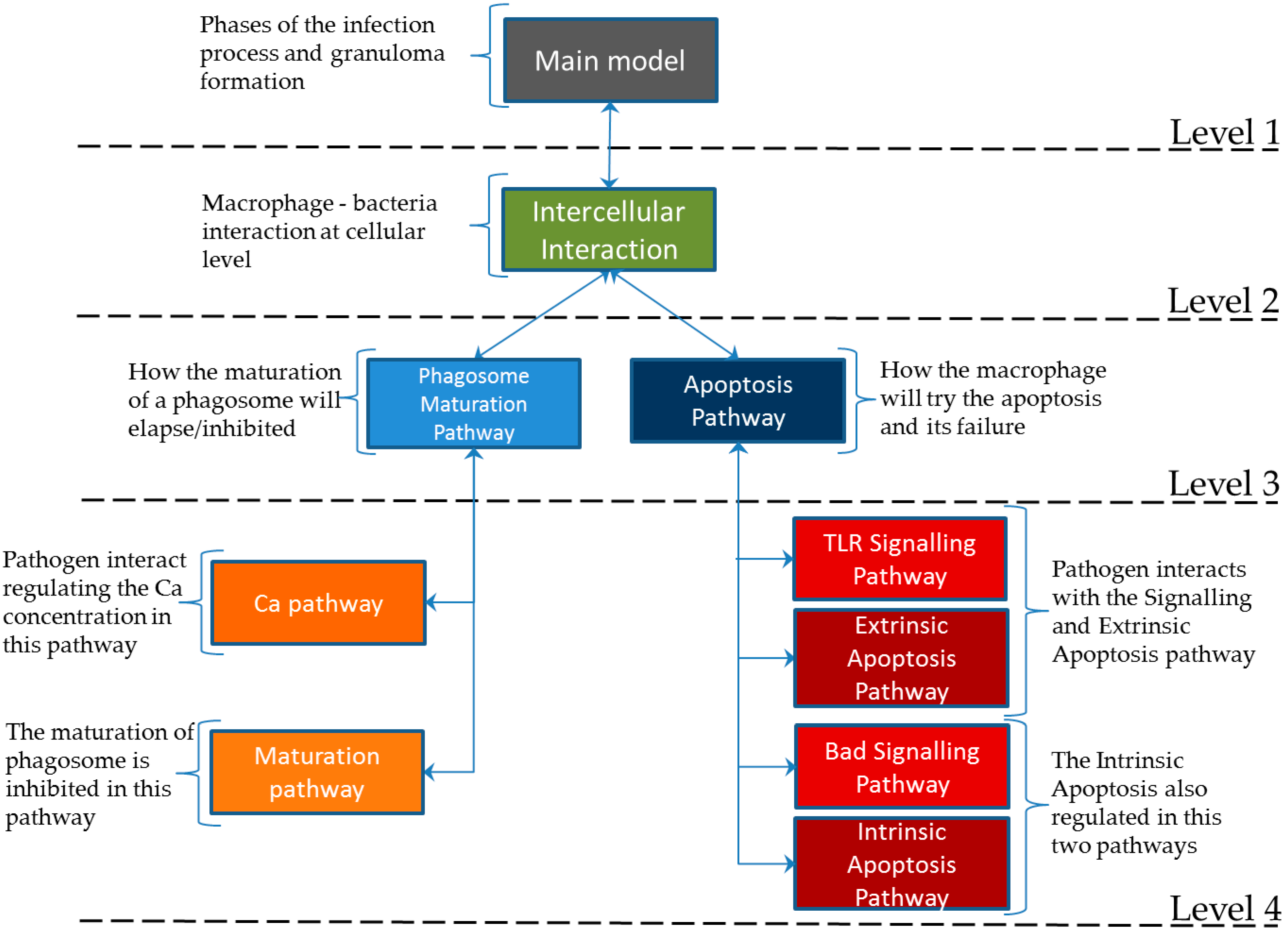
The biological processes described in Section 2.1 occur at different scales, i.e., the molecular, the cellular, and the tissue level. Therefore, in this study, we have designed our qualitative colored Petri net model in a hierarchical structure with four different levels of representation. The model reproduces the dynamics of the steps that are involved in the infection process and innate immune response. It also models the signaling pathways activated by macrophages in response to bacteria and how the bacteria explore this to proliferate. The implemented levels operate as containers, where level 1 represents the large-scale model that contains the entire small-scale model. The information flow is triggered on the top level but eventually flows in both directions (top–down and bottom–up). 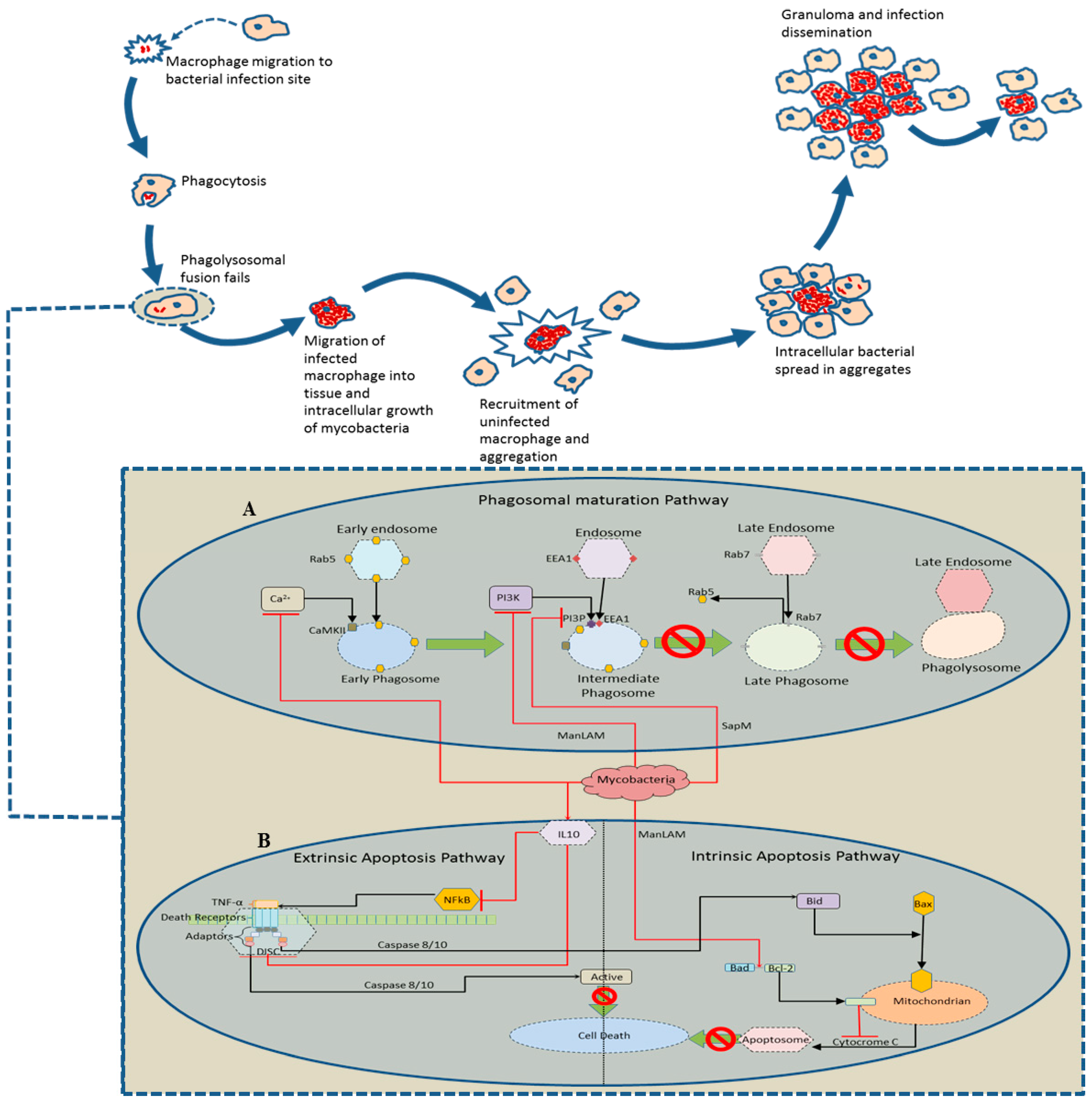Figure 3 depicts the hierarchical structure of the net. Level 1 provides a model for the phases of the infection process: infection detection and phagocytosis, phagolysosome failure, bacterial proliferation, migration of infected macrophages to deep tissue, death of macrophages, recruitment of new immune cells and granuloma formation, intracellular spread, and granuloma dissemination. At level 2 we have modeled the bacteria and macrophage interaction on the intercellular scale. This is directly connected to level 3, in which we model the interactions at the intracellular scale; here, the important pathways related to the bacterial proliferation are modeled. At level 4 we have assembled the important interactions (from the molecular perspective) influencing the infection process.

Figure 3. Hierarchical structure of the model. The levels are implemented as independent and interconnected subnets, following the structure of [23].

Figure 3. Hierarchical structure of the model. The levels are implemented as independent and interconnected subnets, following the structure of [23].

Snoopy supplies features for the design and systematic construction of larger Petri nets. In hierarchically structured nets, coarse places and coarse transitions hide place-bordered (transition-bordered) subnets. Through these, it is possible to zoom in the model to a specific submodel and check a local behavior.

In the following sections, we present the color-set $\text{Σ}$, places $P$, transitions $T$, and the initial marking $\text{I}$ from the main model i.e., level 1 as well as the coarse places and transitions that compose our hierarchical structured model, a qualitative colored Petri net specified as $\left(\text{Σ},P,T,A,C,G,E,I\right)$.

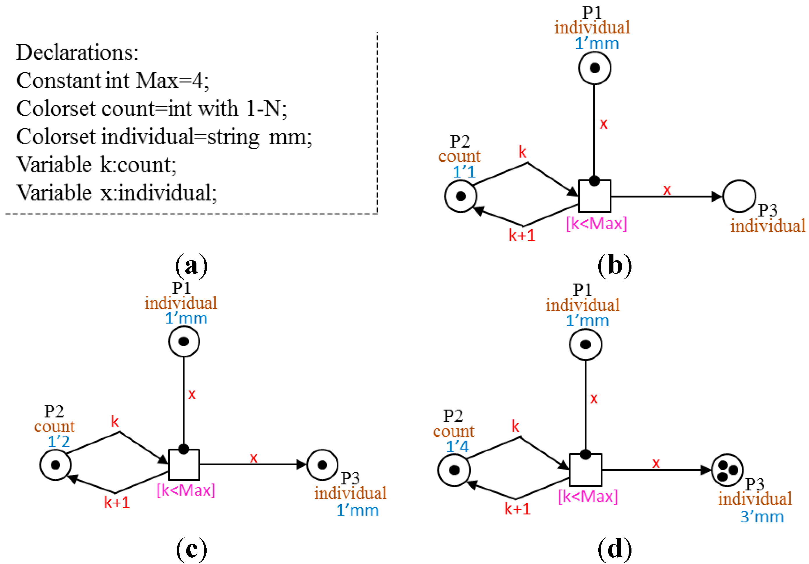
3.1. Set of Color-Sets Σ

The set of color-sets from [22] is extended with a new color-set, Dot. This is a color-set with only one element as a color. It is used to define discrete numbers of markings that represent the presence or absence of a molecule, protein or cell in the sublevels of our model. Table 1 describes the five simple color-set defined in our model. We introduce three compound color-sets as product of simple, predefined color-sets. Table 2 describes the compound color-sets of the model.

Table 1. Simple color-sets defined for the colored Petri net model.

	Color-Set	Data Type	Description
1	position	Integer	Represents a location (of a macrophage, bacteria, and/or granuloma) within the zebrafish embryo
2	individual	String	Distinguishes bacteria and macrophages (Mm, Mac), respectively
3	status	Boolean	Represents the infection status of a macrophage, i.e., healthy = true; infected = false
4	count	Integer	Represents a threshold for the simulation in the recruitment of macrophage and the dissemination of a granuloma
5	Dot	dot	Default black color, used to evaluate a condition being true or false for a specific molecule or protein, or to count a number of cells

Table 1. Simple color-sets defined for the colored Petri net model.

	Color-Set	Data Type	Description
1	position	Integer	Represents a location (of a macrophage, bacteria, and/or granuloma) within the zebrafish embryo
2	individual	String	Distinguishes bacteria and macrophages (Mm, Mac), respectively
3	status	Boolean	Represents the infection status of a macrophage, i.e., healthy = true; infected = false
4	count	Integer	Represents a threshold for the simulation in the recruitment of macrophage and the dissemination of a granuloma
5	Dot	dot	Default black color, used to evaluate a condition being true or false for a specific molecule or protein, or to count a number of cells

Table 2. Compound color-sets defined for the colored Petri net model.

	Color-Set	Product Type	Description
1	Bacteria	position, individual	Represents the M. marinum bacteria that are modeled
2	Macrophage	position, individual, status	Represents host macrophage immune cells
3	Granuloma	position, individual, count	Represents granuloma with a number of infected macrophages

Table 2. Compound color-sets defined for the colored Petri net model.

	Color-Set	Product Type	Description
1	Bacteria	position, individual	Represents the M. marinum bacteria that are modeled
2	Macrophage	position, individual, status	Represents host macrophage immune cells
3	Granuloma	position, individual, count	Represents granuloma with a number of infected macrophages

3.2. Set of Places P

Places represent a population of cells and multicellular complexes that are integrated in our model. The set of places P that composes level 1 of our model are defined as:

$P=${Infection, ImmuneSystem, InfectionPosition, InfectedMacrophage, ActiveMacrophage, DeadMacrophage, RecruitedMacrophage, FormedGranuloma, MatureGranuloma, MacrophageDisseminated, IntracellularInteraction}

(1)

These places are defined and described in Table 3.

Table 3. Set of places composing level 1 of the model.

	Place	Color-Set	Description
1	Infection	Bacteria	Represent the initial infection site. It contains the initial mycobacteria that intrude the host
2	ImmuneSystem	Macrophage	Represents the immune cells of the zebrafish. It contains the non-infected macrophage cells that respond to an infection or recruitment signaling
3	InfectionPosition	Bacteria	Maintains the information of the initial position of the infection. This is important for the 3D visualization to identify where the infection initially occurs
4	InfectedMacrophage	Macrophage	Represents the macrophage after phagocytosis of bacteria.
5	ActiveMacrophage	Macrophage	Represents the infected macrophage moving in the blood circulation. It shows the macrophage changing its position while the bacteria proliferate
6	DeadMacrophage	Macrophage	Represents the necrotic macrophages positioned in the tissue after been completely infected and signaling to new immune cells to take the infection
7	RecruitedMacrophage	count	Counts/Controls the amount of healthy macrophages that are recruited to form the granuloma
8	FormedGranuloma	Granuloma	Represents the formation of granuloma. It contains the information about the granulomas formed with their specific position and amount of macrophages.
9	MatureGranuloma	Macrophage	Represents the spread of the bacteria inside the granuloma. It contains information about the granulomas, i.e., their positions and amount of macrophages (concentration) of each granuloma
10	MacrophageDisseminated	count	Counts/Controls the amount of infected macrophages that will leave the granuloma to disseminate the infection on another position
11	IntracellularInteraction	Dot	Coarse place that holds the hierarchical subnets, i.e., the connected hierarchical layers in the model and represents the bacterial-macrophage interaction at the intercellular, intracellular, and molecular level, as defined in [23]

Table 3. Set of places composing level 1 of the model.

	Place	Color-Set	Description
1	Infection	Bacteria	Represent the initial infection site. It contains the initial mycobacteria that intrude the host
2	ImmuneSystem	Macrophage	Represents the immune cells of the zebrafish. It contains the non-infected macrophage cells that respond to an infection or recruitment signaling
3	InfectionPosition	Bacteria	Maintains the information of the initial position of the infection. This is important for the 3D visualization to identify where the infection initially occurs
4	InfectedMacrophage	Macrophage	Represents the macrophage after phagocytosis of bacteria.
5	ActiveMacrophage	Macrophage	Represents the infected macrophage moving in the blood circulation. It shows the macrophage changing its position while the bacteria proliferate
6	DeadMacrophage	Macrophage	Represents the necrotic macrophages positioned in the tissue after been completely infected and signaling to new immune cells to take the infection
7	RecruitedMacrophage	count	Counts/Controls the amount of healthy macrophages that are recruited to form the granuloma
8	FormedGranuloma	Granuloma	Represents the formation of granuloma. It contains the information about the granulomas formed with their specific position and amount of macrophages.
9	MatureGranuloma	Macrophage	Represents the spread of the bacteria inside the granuloma. It contains information about the granulomas, i.e., their positions and amount of macrophages (concentration) of each granuloma
10	MacrophageDisseminated	count	Counts/Controls the amount of infected macrophages that will leave the granuloma to disseminate the infection on another position
11	IntracellularInteraction	Dot	Coarse place that holds the hierarchical subnets, i.e., the connected hierarchical layers in the model and represents the bacterial-macrophage interaction at the intercellular, intracellular, and molecular level, as defined in [23]

3.3. Set of Transitions T

The set of transitions T of level 1 of our model is defined as:

$T=${Phagocytosis, PhagolysosomeFail, Migration, MigrationDeepTissue, Recruitment, IntracellularSpread, Dissemination}

(2)

These describe important phases in the infection process and are regulated by thresholds that control the simulation. Table 4 describes these transitions and their guards (if present).

3.4. Initial Marking I

An initial marking defines the number and type of colored tokens that are initially present in a specific place. For the modeling of the Mm infection, we have defined initial makings in our previous work [22]. There exist two types of markings, i.e., (1) condition markings that are fixed and used to control the process; and (2) example markings that are not fixed and can be changed according to the experimentation with the net. Table 5 and Table 6, respectively, describe these types of markings.

All other places in the top-level model, i.e., level 1 of the hierarchical structure, are initially empty, meaning that there are no tokens in these places at the onset of the simulation.

Table 4. Set of transitions composing level 1 of the model.

	Transition	Guard	Description
1	Phagocytosis	-	Fires once its pre-places contain bacteria and immune cells at the same position. It produces tokens that represent infected macrophages as well as tokens that hold information on the initial infection position for the 3D visualization tool.
2	PhagolysosomeFail	-	Responsible for the activation of the intracellular bacterial spread, modeled in the sublevels of the hierarchical structure, while the infected macrophage moves along the blood stream, i.e., changes its position.
3	Migration	-	Responsible for controlling the macrophage position change (movement throughout the blood stream).
4	MigrationDeepTissue	-	Fires once the macrophages reach the threshold within the bacteria migrating to deep tissue to form the granuloma.
5	Recruitment	-	Signals to the non-infected immune cells, i.e., healthy macrophages, to take over the dead macrophage in their specific tissue position, thereby forming the granuloma.
6	IntracellularSpread	-	Represents the maturation of the granuloma by releasing bactericidal material and infecting macrophages that form the granuloma.
7	Dissemination	I ≤ MaxDissemination	Controls the threshold of the amount of infected macrophages that will leave the granuloma and disseminate the infection, forming a new granuloma on a different position.

Table 4. Set of transitions composing level 1 of the model.

	Transition	Guard	Description
1	Phagocytosis	-	Fires once its pre-places contain bacteria and immune cells at the same position. It produces tokens that represent infected macrophages as well as tokens that hold information on the initial infection position for the 3D visualization tool.
2	PhagolysosomeFail	-	Responsible for the activation of the intracellular bacterial spread, modeled in the sublevels of the hierarchical structure, while the infected macrophage moves along the blood stream, i.e., changes its position.
3	Migration	-	Responsible for controlling the macrophage position change (movement throughout the blood stream).
4	MigrationDeepTissue	-	Fires once the macrophages reach the threshold within the bacteria migrating to deep tissue to form the granuloma.
5	Recruitment	-	Signals to the non-infected immune cells, i.e., healthy macrophages, to take over the dead macrophage in their specific tissue position, thereby forming the granuloma.
6	IntracellularSpread	-	Represents the maturation of the granuloma by releasing bactericidal material and infecting macrophages that form the granuloma.
7	Dissemination	I ≤ MaxDissemination	Controls the threshold of the amount of infected macrophages that will leave the granuloma and disseminate the infection, forming a new granuloma on a different position.

Table 5. Condition markings initially defined in the colored Petri net model.

	Place	Marking	Description
1	RecruitedMacrophage	1`(1)	Initializes the counting of the number of macrophages recruited to aggregate into the dead macrophage. It has a threshold defined by a constant MaxAggregation i.e., 5.
2	MacrophageDisseminated	1`(1)	Initializes the counter of the amount of infected macrophages that leave the granuloma and spread the infection to different positions. It has a threshold defined by a constant MaxDissemination i.e., 3.

Table 5. Condition markings initially defined in the colored Petri net model.

	Place	Marking	Description
1	RecruitedMacrophage	1`(1)	Initializes the counting of the number of macrophages recruited to aggregate into the dead macrophage. It has a threshold defined by a constant MaxAggregation i.e., 5.
2	MacrophageDisseminated	1`(1)	Initializes the counter of the amount of infected macrophages that leave the granuloma and spread the infection to different positions. It has a threshold defined by a constant MaxDissemination i.e., 3.

Table 6. Example markings initially defined in the colored Petri net model.

	Place	Marking	Description
1	Infection	1`(1,mm) ++1`(2,mm) ++1`(3,mm)	Defines the initial concentration of mycobacteria that will intrude the host. We have defined three different positions to represent different initial infection sites.
2	ImmuneSystem	1`(1,mac,true) ++1`(2,mac,true) ++…++1`(12,mac,true)	Defines the initial concentration of non-infected macrophages in the host. The positions and amount are empirical information used just to represent their presence in the host.

Table 6. Example markings initially defined in the colored Petri net model.

	Place	Marking	Description
1	Infection	1`(1,mm) ++1`(2,mm) ++1`(3,mm)	Defines the initial concentration of mycobacteria that will intrude the host. We have defined three different positions to represent different initial infection sites.
2	ImmuneSystem	1`(1,mac,true) ++1`(2,mac,true) ++…++1`(12,mac,true)	Defines the initial concentration of non-infected macrophages in the host. The positions and amount are empirical information used just to represent their presence in the host.

3.5. Sub-Models in the Hierarchical Structure

Following the tree of the hierarchical structure, the submodels, implemented through the coarse place IntracellularInteraction, model a complex process involving various host-bacterial factors in a cross-talk interaction distributed in the sublevels. In order to get a consistent view of the entire interaction process, we express the most important reactions by simplifying the pathways at different levels of abstraction. The simplification of the pathways corresponds to our previously defined modeling decisions [23], where each biochemical compound or receptor is defined as a place. The relations between biochemical substances are represented by transitions with corresponding arcs for the reactions. Inhibitions and degradations are represented by inhibitor arcs. Signaling and catalytic atomic events are represented by read-arcs. We specifically use the color-set Dot to represent the presence of a protein, component, and/or cell that is involved in the interaction process between the macrophage and bacteria once it is phagocytosed. To hierarchically connect the different pathways we use coarse transitions and coarse places structuring all the sublevels, as shown in Figure 3.

4. Results

The simulation environment for the model represents the innate immune response to M. marinum infection in the zebrafish embryo. The elements of the qualitative colored Petri net described in the previous sections represent key factors involved in the processes of infection, innate immune response, and granuloma formation. Moreover, the interactions are represented by the firing rules that describe the behavior of the model:

(i)

Signaling of the intruding bacteria, detected by non-infected macrophages followed by phagocytosis;

(ii)

Migration of the infected macrophage to the deep tissue within bacterial replication motivated by the phagolysosome failure in the macrophage, causing the cell death;

(iii)

Recruitment of non-infected macrophage in response to signals of the dead macrophage, clustering to form the granuloma;

(iv)

Granuloma maturation and bacterial spread between aggregated macrophage;

(v)

Infection dissemination through infected macrophages that escape from the matured granuloma, forming new granulomas at different positions.

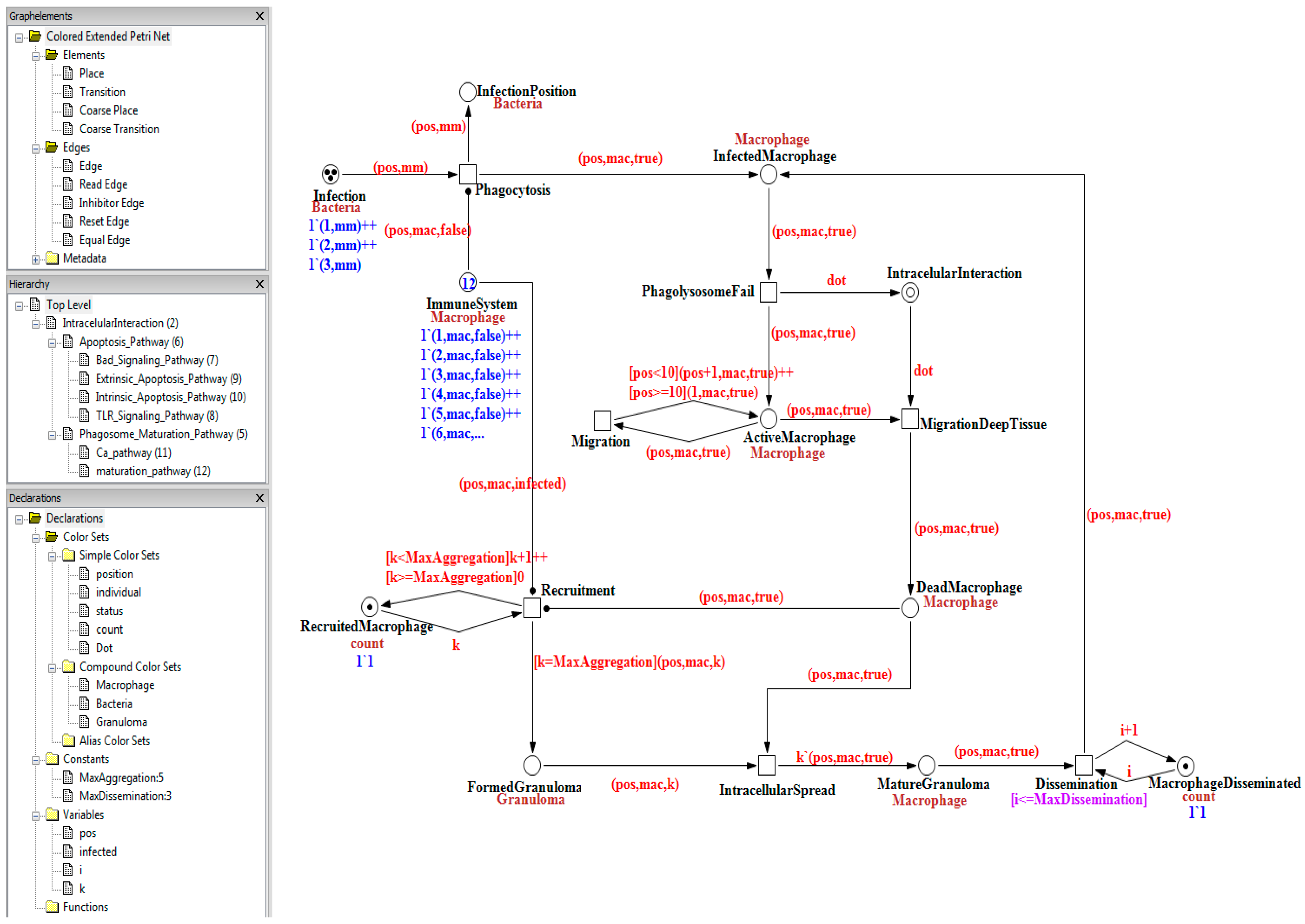
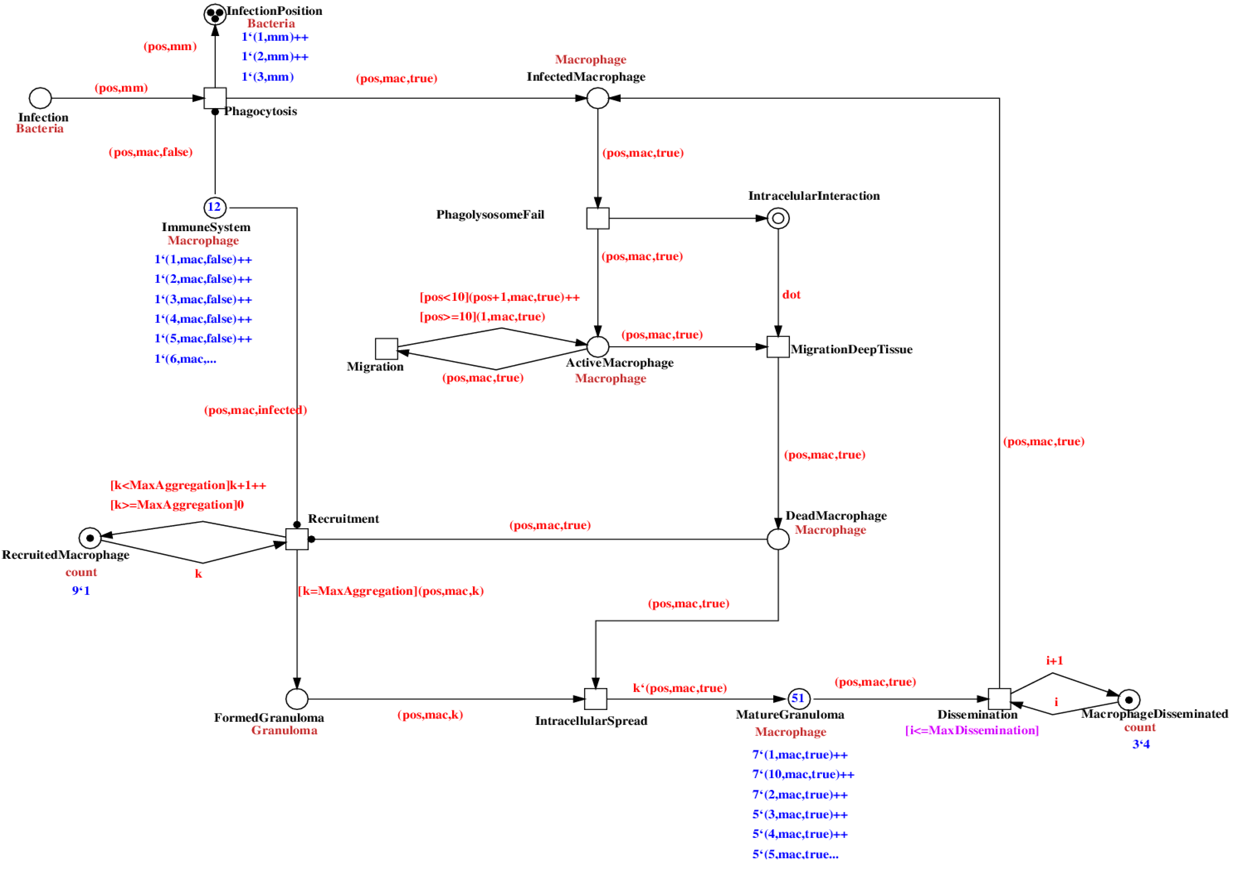
The top-layer level of our model is depicted in Figure 4. Places are represented by circles and coarse places by double circles. Transitions are represented by squares and coarse transitions by a double square. The number of tokens is expressed inside the places and their dataset below the color-set (cf. Figure 4, dark blue). Arrows represent the arcs labeled with their expression on top of it (cf. Figure 4, light red). The arcs with a black dot as an arrowhead are read arcs. In the notation of our PN software environment, these are represented as two arcs in opposite directions between place and transition with an identical arc expression. However, the tokens are not consumed, just tested for their presence.

Figure 4. Visualization of the qualitative colored Petri net model implemented in the Snoopy framework [44]. In the left panel, information about the Petri net model is displayed: the hierarchical structure and definitions used in the model, the color-set, the constants, and variables. The main panel shows level 1 (cf. Top Level) of the hierarchical Petri net model and its properties.

Figure 4. Visualization of the qualitative colored Petri net model implemented in the Snoopy framework [44]. In the left panel, information about the Petri net model is displayed: the hierarchical structure and definitions used in the model, the color-set, the constants, and variables. The main panel shows level 1 (cf. Top Level) of the hierarchical Petri net model and its properties.

In the model, the data value of the colored Petri net formalism is used to represent the quantities that change during the simulation. Although our focus is on a qualitative model, the quantitative aspects promote a better interpretation of the dynamical aspects of the simulation. Level 1, depicted in Figure 4, models the different stages of the infection process. It represents the phases of injection, phagocytosis, migration, granuloma formation, and dissemination. 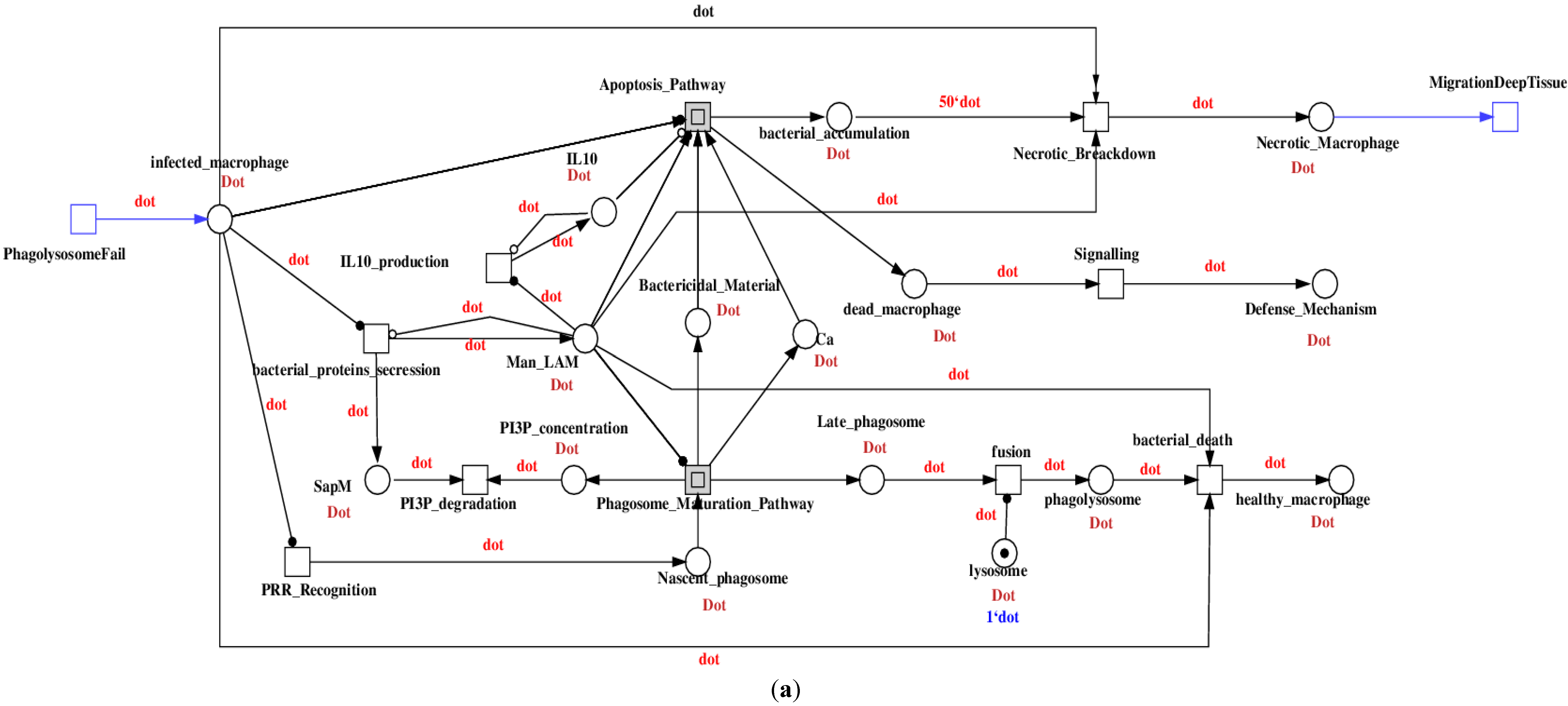Expanding the hierarchical structure, the connection of the sub-models and their components are depicted in Figure 5. Level 2 is modeled in the coarse place IntracelularInteraction of level 1 (cf. Figure 4). It represents the intercellular interaction between mycobacterium and a macrophage and is triggered by the phagolysosome fail (cf. Figure 5a). Level 3 models the intracellular interaction, represented by the coarse transitions: Phagosome_Maturation_Pathway (cf. Figure 5b) and Apoptosis_Pathway (cf. Figure 5c). These course places bridge the signaling started at the cell wall (cf. level 1) that triggers the interactions between molecules. Level 4 models the molecular interaction of the proteins released by the bacteria and the proteins from the macrophage. They are represented by the coarse places Extrinsic_Apoptosis_Pathway, Intrinsic_Apoptosis_Pathway, Ca_Pathway, Maturation_Pathway, and also the coarse transitions Bad_Signaling_Pathway and TLR_Signaling_Pathway.

We have defined some boundaries to limit the model for a better qualitative analysis of the behavior of the system. The intracellular bacterial proliferation is defined by the arc expression 2`dot, which represents the offspring of two new bacteria every time the transition $T=${bacterial_proliferation} fires (cf. Figure 5b). The capacity of the infected macrophage is limited to a concentration of 50 bacteria. After the place $P=$ {bacterial_acumulation} reaches this boundary, i.e., arc expression 50`dot, the transition $T=$ {Necrotic_Breakdown} can fire. This action changes the infected macrophage into a necrotic macrophage that will leave the bloodstream and migrate into the tissue (cf. Figure 5a).

Another threshold used is related to the position of macrophages and granulomas. Nezhinsky et al. [45] have developed an image processing platform for the analysis of high-throughput screens in zebrafish. In this platform, infected zebrafish embryos are automatically recognized as a shape. Relative to the shape, the bacterial infection is analyzed as an infection spread; to this end, the shape is divided into 12 regions of infection. This research has inspired us to determine 12 relative positions based on this division to model the presence of the macrophages, their movement during the infection process, and also the spread of the granuloma. The concentration of aggregated macrophages is limited by setting a constant called MaxAggregation. Moreover, the infection dissemination is limited further by setting a constant MaxDissemination (cf. Figure 4). We use these thresholds to control the amount of cells that form the granuloma, as well as the number of dissident infected macrophages that are released from the granuloma to spread the infection to other positions.

The outcome of our model reproduces the early stages of the mycobacterial infection process and innate immune response. We use the animation mode available in the Snoopy framework to verify the dynamic behavior of our model. This property enables the animation of token flow through the net, in order to observe the causality of the model and its behavior on the whole hierarchical structure. To show the importance of the immune cells, molecules, and processes in the dynamics of the infection, we performed a simulation based on our specific experimental scenario, defined in Section 2.1.

Figure 5. Submodels in the hierarchical structure: (a) Level 2: Intercellular interaction between bacteria and macrophage. (b) Apoptosis_Pathway and (c) Phagosome_Maturation_Pathway represent the intracellular interaction positioned at level 3. Level 4 represents the molecular interactions defined in [23]; they are modeled in the coarse places and coarse transitions (data not shown).

Figure 5. Submodels in the hierarchical structure: (a) Level 2: Intercellular interaction between bacteria and macrophage. (b) Apoptosis_Pathway and (c) Phagosome_Maturation_Pathway represent the intracellular interaction positioned at level 3. Level 4 represents the molecular interactions defined in [23]; they are modeled in the coarse places and coarse transitions (data not shown).

We start the simulation by defining the amount of bacteria and their initial position at the place of infection, adding the initial markings: $I${1`(1,mm)++ 1`(2,mm)++ 1`(3,mm)}. The ImmuneSystem place, which contains macrophages, sends to the initial infected position a non-infected macrophage to phagocytose the bacteria. The macrophage becomes infected through a failure of the phagolysosomal process. Next, in the sublevels of the net the proliferation of bacteria will occur while the infected macrophage is migrating along the blood circulation. In the net, the proliferation process is triggered by sending a token 1`dot, to the coarse place IntracelularInteraction. At level 2, the infected macrophage attempts to kill the bacteria by activating the phagosome maturation or apoptosis process. The signaling process starts by sending a token from the place Nascent_Phagosome to the coarse transition Phagosome_Maturation_Pathway, and from the place Bactericiadal_Material to the coarse transition Apoptosis_Pathway. At level 3, these pathways trigger molecular interaction, by sending tokens to the coarse places and coarse transitions that model the protein–protein interactions at level 4. The bacteria interact with both pathways by releasing the ManLAM as presented by the place Man_LAM. It escapes being killed and instead proliferates inside the macrophage (cf. place Bacterial_acumulation), causing a macrophage necrotic breakdown. At this moment the necrotic macrophage leaves the blood circulation (at level 1) and migrates to deep tissue. There it will recruit non-infected macrophages to form a granuloma (cf. place Formed_Granuloma). The bacteria will spread inside the granuloma, and will disseminate the infection by releasing an infected macrophage into the blood circulation. These processes repeat for each infected macrophage that leaves the granuloma.

The amount of infected macrophages leaving the granuloma is limited through the constant MaxDissemination. Once this threshold is reached, no further transition is enabled to occur and the execution will terminate in its final state. Since our model is focused on the qualitative aspects of the bacterial infection process and innate immune response, we bound our simulation by this constant to represent the initial dissemination of the infection. The final state then provides the quantity of granuloma formed during this process and their respective positions, accumulated at the place MatureGranuloma. In Figure 6 the final state of the net is depicted; an animation sequence of this PN can be found in [46]. By saving the final state result of the CPN it becomes possible to derive the complete state space from the Petri net file. This file is subsequently used as the input for the 3D visualization of the process. The Snoopy file can be obtained upon request.

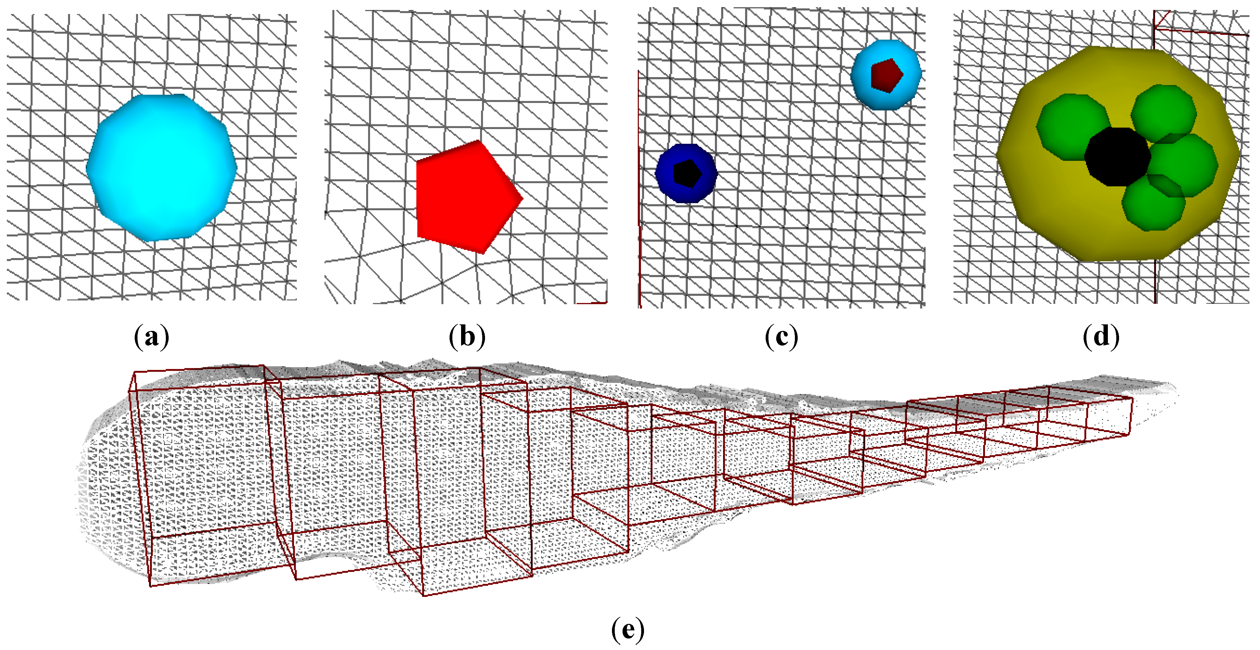
The 3D visualization tool was built to provide an alternative animation of the Petri net. We defined graphical elements to represent bacteria, macrophages, and granulomas, whereas a 3D mesh object represents the zebrafish embryo. The 3D visualization of the infection process plays the exact same simulation as the animation of the colored Petri net model. We define 12 regions in the mesh to represent the positions where infection can occur. The positions are relative to spatial enumerations in the zebrafish model and normalized to its total length. The 3D animation is played over the entire volume of the 3D mesh. The 3D animation visualization software arranges the positioning of the objects in such a way that there is no overlap between the objects, nor do they mutually collide. In Figure 7, the graphical elements and the object environment of the 3D visualization are depicted.

Figure 6. Animation mode at its final state, where there are no more enabled transitions to occur. We save this state and use the file as input to our 3D visualization tool.

Figure 6. Animation mode at its final state, where there are no more enabled transitions to occur. We save this state and use the file as input to our 3D visualization tool.

Figure 7. 3D visualization tool and its elements: (a) Macrophage; (b) Bacteria; (c) Infected macrophages; (d) Granuloma; (e) Fish embryo with the 12 regions where infection can occur.

Figure 7. 3D visualization tool and its elements: (a) Macrophage; (b) Bacteria; (c) Infected macrophages; (d) Granuloma; (e) Fish embryo with the 12 regions where infection can occur.

In the 3D animation, the initial bacteria are introduced according to the information of the Petri net model. It reads the colored tokens in the place InfectionPosition, normalizing the position values and placing the bacteria objects in the predefined regions accordingly. In the Petri net model, the non-infected macrophages are in all of the 12 possible regions as they are transported through the blood vessels. The granuloma formation and dissemination occur on the basis of the information from the colored tokens as present in the place MatureGranuloma. The constants MaxAggregation and MaxDissemination bound the infection process. The animation is time-independent and sequentially follows the infection steps as defined in the model. The 3D animation renders the dynamics of infection process and granuloma formation according to the final state space from the Petri net. For inspection and perusal, an animation sequence can be found in [46]. 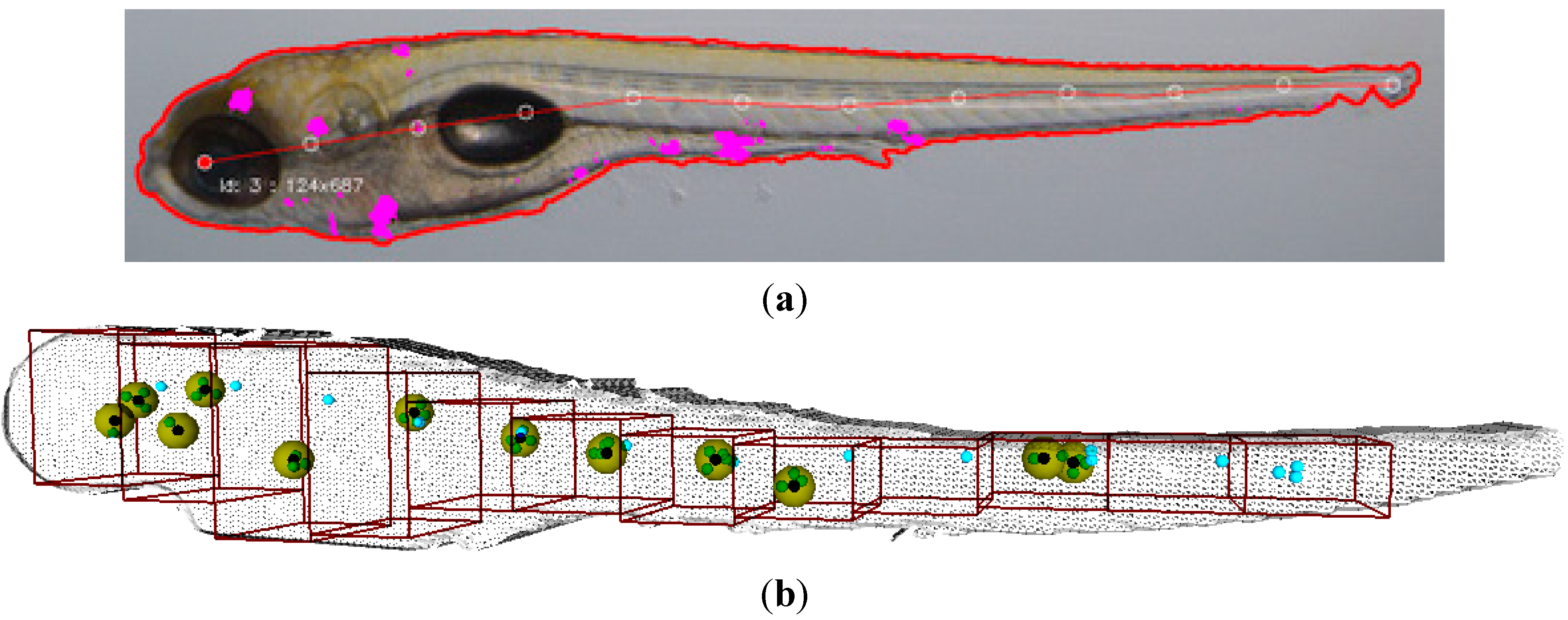In Figure 8a comparison is provided of the 3D visualization with the Petri net data with a real zebrafish embryo that has been infected with Mm. The microscope image of a seven-day-old zebrafish depicted in Figure 8a is the result of an analysis for the spread of the Mm bacteria after six days of infection (dpi). This result was obtained with specific software and the granulomas extracted from the image are overlaid as magenta blobs [27,45]. The final result of the 3D animation visualization is depicted in Figure 8b. As one can appreciate here, the simulation reproduces the distribution of the granulomas resulting from the infection process along the fish, in a similar pattern as occurs in the real zebrafish. Therefore, it is possible to correlate our final result with in vivo experiments although we are not using quantitative data. The threshold for manipulating the dynamics of the CPN model is the only quantitative information that has been used, and this threshold is not directly based on the analysis of empirical data. We, therefore, cannot directly compare the amount of granuloma or the distribution of the infection as obtained from our CPN model to in vivo situations. However, we can extrapolate from the results of our simulation that the structure of our Petri net model qualitatively represents the behavior of the in vivo infection process.

Figure 8. (a) Microscope image of a seven-day-old zebrafish (7 dpf) infected with wild-type Mm bacteria one day old, referred to as six days post-infection (6 dpi). The granulomas are displayed as magenta blobs. (b) The end state of the 3D animation with all the granulomas formed according to the final state space of the colored Petri net model.

Figure 8. (a) Microscope image of a seven-day-old zebrafish (7 dpf) infected with wild-type Mm bacteria one day old, referred to as six days post-infection (6 dpi). The granulomas are displayed as magenta blobs. (b) The end state of the 3D animation with all the granulomas formed according to the final state space of the colored Petri net model.

5. Conclusions and Discussions

The model we presented in this work is concerned with an infection scenario: the innate immune response to M. marinum in zebrafish. It represents the dynamics of bacterial proliferation, granuloma formation, and dissemination. The model captures the relevant functional processes and their interconnections, including signaling and activation or inhibition of the immune responses at different levels of abstraction. In sublevels, we have connected the most important pathways in order to model the response of the macrophage on the exposure to pathogenic mycobacteria. Information about the proteins released by the bacteria, their interference with the immune response, and the pathways involved in this process are also taken into account.

We focused on modeling the qualitative aspects of the infection process through connecting two complementary models: one for the reaction process and biochemical components implemented as a qualitative Petri net (without colors) [23]. The other model [22] represents the dynamics of the cells in the infection process, which is implemented as a colored Petri net. The resulting hierarchical Petri net model covers the relevant phases of the infection process, as well as the interaction pathways related to the infection persistence.

In order to combine the two models into one net model, the QPN model [23] was first converted into a QPN^C model. The color-set Dot was introduced to represent the presence of signaling molecules, proteins, and concentrations of cells involved in the interaction between macrophage and bacteria that are phagocytosed. Through this color-set, the two models were combined in one modular structure. Using the Snoopy platform in animation mode, the combined hierarchical model could be executed.

The animation mode of Snoopy allows one to verify the dynamics of an animated Petri net by analyzing the markings encountered during a simulation. This showed that our Petri net model was able to replicate the steps in the infection process. This is due to the fact that the structure of the Petri net is based on the actual description of the infection process as extracted from the literature. Hence, the qualitative aspects in the sense of cause-and-effect are in accordance with the actual process. The quantities used in the model have no direct significance but to support the qualitative modeling and serve only as threshold. Neither quantities nor time are essential to the working of the model.

From a biological perspective, the additional 3D visualization environment has proven to be an interesting complementary approach to illustrate the infection process. The possibility of visualizing the infection, from the introduction of bacteria to granuloma formation as it would happen in vivo, provides a better understanding of the infection process.

A comparison of the simulation results with an in vivo experiment (an infected zebrafish at 6 dpi) confirms once more the strength of the qualitative aspects of our model (cf. Figure 8).

Because the 3D visualization tool reads markings of the Petri net model, changes in the initial marking of the net are directly reflected in the 3D visualization. Thus it can lead to more insight into the infection process, e.g., how dissemination and concentration of granulomas depend on the initial position of the bacteria, the amount of aggregation cells that form a granuloma, as well as on the number of infected macrophages that can leave the granuloma. By changing the number and/or positions of tokens, “what-if” scenarios can be executed to represent different biological conditions. Disruptions of pathways, the presence or absence of proteins, and also different positions of cells can be simulated as part of the experimentation in the animation mode.

For the further development of “what-if” scenarios, however, a quantitative model is necessary that, through support of empirical data, would enable us to do quantitative analysis as well as perform simulations and predictions. An advantage of our Petri net model is its modularity, facilitating the conversion from a qualitative model to a quantitative model without changing the structure. Since the 3D visualization can perform an animation based on the final state space of the net, it would then provide an even more realistic perspective of the infection process. Currently, we are collecting and analyzing data from zebrafish infection studies to use these as a basis for such a quantitative model. As a next step, we will integrate these data in our simulation framework and will then be able to perform different scenarios as part of the simulation process. This will contribute to identifying important parameters that can help to unravel mechanisms related to the mycobacterial infection process and innate immune response.

In summary, in this paper, we have presented the coupling of two distinct models of different aspects of the mycobacterial infection process and innate immune response. To understand infection and the immune response, it is necessary to analyze the process from its epidemiology down to genetic levels. We have modeled the dynamics of the infection and also the intracellular, intercellular, and molecular interactions, interconnecting the models in a hierarchical structure. The resulting multi-scale Petri net model allows for the observation of events at a given scale and how they interact with higher or lower levels. In addition, we provided an animation of the model using the Snoopy framework and related the Petri net output to a 3D environment. The hierarchical structuring of information in Petri net has the potential to become an important tool for research into infectious diseases, tuberculosis in particular.