1. Introduction
The application of mathematical models to human societies has a long history [
1,
2,
3,
4,
5,
6]. Such models typically enable one to cast verbal arguments into a quantitative form and see how they play out over various scenarios. In this way such arguments can go from being “reasonable” to being “testable”, and, if not provable, at least falsifiable. One of the most powerful benefits of such generic, simple models arises when they fail to reproduce known historical details. In a complicated model, it is usually possible to fix discrepancies by refitting the values of the parameters. In a simple model there is little scope to do this: the discrepancy indicates an effect which was important in that particular application.
One of the more puzzling aspects of history is that the human population has grown steadily, either since emerging from Africa [
7] or at least through recorded history and since the proposed genetic bottleneck 50,000 years ago [
8,
9]. Clearly this is due to the population approaching the carrying capacity of the earth and extending it by environmental modification. A simple model for this would show monotonic expansion. However, during this period, individual cultures have risen and fallen. A simple model for this process should show both growth and collapse,
and be extendible to explain the overall growth.
Ignoring spatial effects, it is standard to describe population growth (N) to a fixed carrying capacity () using the logistic expression which gives initially exponential growth, subsequently slowing to saturation where τ is a characteristic time, similar to one generation. To incorporate environment improvement/degradation an additional equation is needed for . We investigate several classes of candidates for this additional equation, and show that they give neither stable solutions nor supraexponential growth. This is then related to the growth and collapse of civilizations.
Many previous works have introduced a spatial dimension. One of the most prevalent of these is Fisher’s reaction-diffusion equation [
10,
11], which gives rise to a “Wave of Advance” of cultural developments, the classic case being the arrival of Neolithic farming in western Europe [
12,
13,
14,
15,
16]. Here, the model borrowed ideas from theoretical biology and showed that the required diffusion and logistic growth parameters required to match the archaeological data for wave speed were reasonable. The model was similarly used to describe the spread of Indo-European languages [
17].
In previous papers, we have derived a similar Wave of Advance equation from more fundamental concepts of food production, birth and death rates for various cultures [
18,
19,
20]. We showed how some cultures could expand at the expense of others. In the case of neolithic farming, the form of the equation is similar to Fisher’s, but since it was derived rather than postulated, it was also possible to deduce more subtle features. In particular, the equations only allow for a wave of advance of farming if the farmers have a birthrate higher than that of the mesolithic hunters and gatherers they are displacing or absorbing. This may be due to their more sedentary lifestyle making childcare easier, a hypothesis which is borne out by observation in contemporary farming and nomadic societies. More unexpectedly, the model required that farmers should be less well nourished and have shorter lifespans than the hunter gatherers they displaced, showing that the strategy more successful for advancing the culture may not be better for the individuals practising it [
19].
An example of the insight gained from failure of a simple model is the importance of riverine transport. The Fisher model applied on a detailed geography of western Europe [
19] fails to account for the known rapid expansion of the neolithic along the Danube-Rhine corridor. This is fixed by higher mobility, modelled as increased diffusion rates along waterways [
19,
21,
22,
23]. Another failing of the Fisher model is that it shows farming arriving in Ukraine from the west, which is inconsistent with the archaeological record. This can be attributed to a bottleneck at the Bosphorus A stochastic version of the model, treating the population as a collection of individuals rather than a continuous quantity, showed that the wave slowed at bottlenecks, and that there is significant uncertainty about how long it would take to pass through. A deterministic model is less reliable here [
24].
A curious feature of mathematical approaches in population dynamics is the use of equations with stable solutions (logistic growth) or limit cycles (Lotka-Volterra). This can lead to a misapprehension that populations are intrinsically stable. We show that if coupling to the environment is incorporated, instability is the normal state of affairs. In general, such nonlinear coupling introduces equations without analytic solution: the unstable cases present the very problems where computation becomes essential. Thus simplified models of social phenomena can yield valuable insight, provided the simplification is done by ignoring minor effects rather than insisting on an analytically-solvable model.
The paper is organised as follows. In
Section 2 we present simple models for the coupling of population to environment, and show they allow only boom-and-bust type solutions. These models are consistent with the history of individual societies, but incompatible with the steady growth of world population. In
Section 3 we present a partial resolution, where a self-repairing natural environment maintains a steady global population. In
Section 4 we present a more credible resolution. In it multiple competing cultures rise and fall in competition, while the carrying capacity and global population rises steadily through innovation.
The central issue in the paper is modification of the environment. Henceforth, whenever we use the word “modification”, it should be understood as referring to modification of the environment.
2. Population Dynamics Coupled to the Environment
The growth of populations has been well described by the logistic equation. More detailed derivations give a more subtle interpretation of the basic parameters, but there seems no reason to use any other equation as a starting point.
where
is the population of
culture at a given region,
τ a timescale typical of a generation,
the total population in the region, and
a measure of the quality of the land. The parameters depend on the culture and technology of the population in question, and the form of the equation allows for spatial variation of
.
The society or culture is defined by the set of parameters τ (and later D, G and A). We define evolution of a culture as a process in which some of these parameters can change slowly and continuously in time, driven by “natural selection”, which favours parts of the culture having higher reproductive success.
2.1. Environmental Modification—One Population (), Homogeneous Terrain
In the absence of environmental change, the stable solution to the Fisher equation is simply
, so
specifies how large a population the land can support.
is the main quantity affected by environmental modification. Let us first assume that the population has two effects on the environment: a positive one through innovation (e.g., irrigation and fertilizers) and a negative one through overpopulation. These can be combined into a single equation for the change in
,
in which
a is the ratio between the population level beyond which population number declines (“carrying capacity”) and the level at which the environment becomes degraded (sometimes called “relative carrying capacity”). It therefore measures how environmentally-friendly or sustainable a culture is. For
, the saturation population degrades the environment faster than it improves it.
G is the rate of environmental modification per person. The factor
means that at low population, modification is proportional to the number of people. Ignoring spatial variation, we can eliminate time dependence from Equations (
1) and (
2):
The behaviour of this two-parameter equation already captures the typical behaviour of various societies. Detailed mathematical analysis of this equation is given in the
Appendix. In
Figure 1 we show the allowed paths through
N,
space as time advances. This turns out to have remarkably rich behaviour. Typically, there are three regions in the
diagram (
Figure 1), separated by the straight lines
(separatrices, see
Appendix) The trajectories cannot cross these lines. The slopes of the separatrices depend on the ratio of timescales of reproduction
τ and modification
. Most notably, there is
no stable solution (Apart from the exceptional case where
a is precisely equal to 1 and
, when
is marginally stable). There are two general cases
and
.
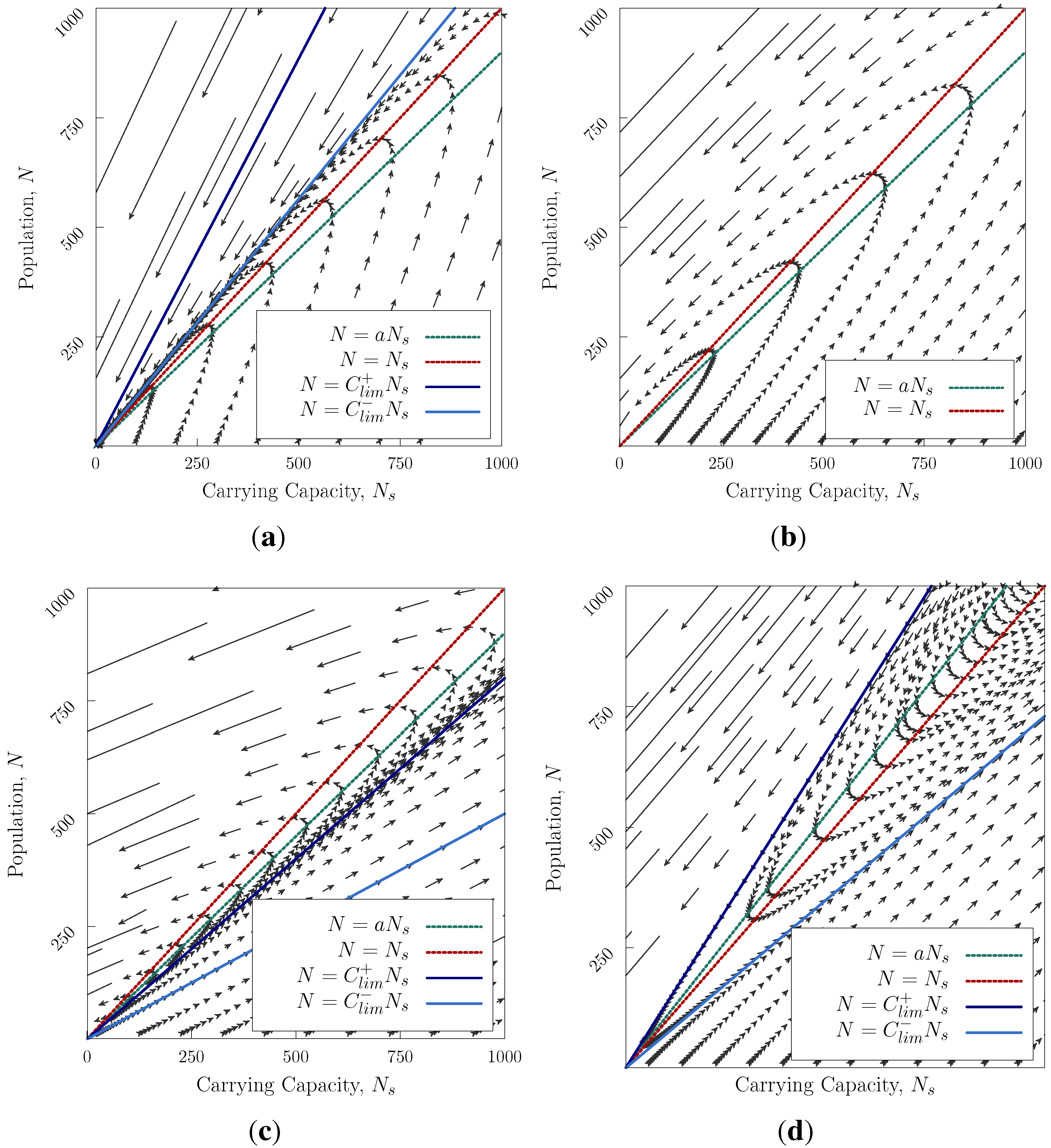
For
,
Figure 1a–c corresponds to the cases where at saturation population, the culture degrades its environment, e.g., by food being produced by unsustainable methods. The arrows show the rate at which the system moves along its trajectory. Realistic cases are those where the society starts with small population. There are three sub-cases, depending on the value of
, which can be interpreted as the ratio of the rate of population growth to the rate of modification of the environment. We can set
G = 1 and still examine all possible cases.
Figure 1a is the case where the population grows rapidly. In the normal case with initially small
N the culture’s history is characterised by a rapid initial expansion, a long mature phase at high population, followed by a collapse which is initially slow, but accelerates viciously as the environment deteriorates through overpopulation (bottom right triangle). If a culture like this was initiated with a large population, or suffered an external environmental collapse to low
, it would collapse very quickly (upper right triangle).
Figure 1b is the case where the population growth and environmental change happen at similar rates. Now there is only one possible trajectory: rapid initial growth, a long period of high population, followed by rapidly accelerating collapse.
Figure 1c is the case where the environmental change is much faster than the population growth. There are now three possibilities: if the population begins at low
N, it can improve the environment so fast that the population never reaches saturation. In this case, the population grows slowly, but without bound. In cases where the culture begins with a population below, but close to, saturation, the population will initially grow to saturation, then the effect of
causes the environment to deteriorate, and the population collapses. If the initial populations is above saturation, collapse occurs immediately.
Figure 1.
Trajectories in
space for Equation (
3), arrows point forwards in time. (
a) The saturation lines
and
have a higher slope than
. In the two upper areas, the system may only decay. In the lower region, the population grows then collapses
,
and
; (
b)
do not exist. The population grows until reaching the saturation line
then declines after crossing the line
.
,
,
; (
c) The saturation lines have a smaller slope than
. In the two lower areas, the system grows exponentially.
,
and
; (
d) The saturation lines lie between
.
,
and
, three regions correspond to collapse, recovery and continual growth.)
Figure 1d is the solution for
. This case corresponds to a society that can continually improve its environment, even once the population reaches saturation level, because degradation initiates only at population levels above saturation. Now for any case where the initial population lies below the upper separatrix, the population will ultimately grow without limit, although there will be an initial decline if the initial population lies above
. For excessively high initial population, or sudden external environmental change, collapse is still inevitable.
Thus the fate of a society depends both on its rate of expansion, compared with environmental improvement, and on its conduct once saturation is reached: whether or not it still continually improves the environment. In either case, the model has no stable solutions: either collapse eliminates the population, or the population grows by achieving a continuous increase in carrying capacity
. This case would give exponential growth, slower than the supraexponential growth exhibited by the human population [
3,
4,
6].
The coupled model suggests that it is impossible to disentangle “overpopulation” from “self-inflicted environmental damage” as a single cause. In famous cases such as Mesopotamia and Easter Island, while environmental collapse appears, there is also overpopulation: as the carrying capacity () decreases, the relative overpopulation increases, even if the population itself is decreasing (N).
The figures also illustrate the resiliency of the system to external shocks. A typical example would be a sudden change in
due to an external environmental event, although a change in
N through civil war or plague is also possible. When this happens, the system jumps from one trajectory to another. The system is resilient if it remains within the same segment in
Figure 1; it will move to a different post-disturbance trajectory in a different environment, but with broadly similar characteristics. On the other hand, if the disturbance takes the system across one of the
lines, a qualitatively new trajectory will be followed. The resilience of the system depends both on its current state and the strength of external shock. The model opens the possibility of simulating famous collapses such as the Greenland Norse, Maya and Anasazi, which have been linked to external climate change (degradation of
).
The stably growing solutions might represent cultures such as ancient Egypt and China. Here, the rate of population growth must be slow (Egyptian population is believed to have doubled in 1000 years, China being similar [
25,
26]).
It is worth noting that in the analysis so far, migration of the population is ignored, or, equivalently, assumed to be fast compared to the timescales of environmental change and population growth. The concept of Wave of Advance is relevant only insofar as that on reaching new terrains the culture can “start again” at low
N and finite
. In principle, a single spreading culture can be at different positions in the
space at different locations and times. In practice, the effects of migrations from overpopulated areas will change the details of the behaviour: this would require more detailed description of what the driving force for migration is [
18,
19]. However, each area will still follow the same broad trajectory to exponential growth or collapse, as determined by the values of
a and
which define the culture.
2.2. Two Populations in Competition
We have established that only populations which invest in improving their environment faster than increasing their population can avoid the Malthusian catastrophe of collapse in the long term. We now consider whether such a sustainable population can survive in competition with a faster growing one,
i.e., whether the strategy which gives an expanding population is an evolutionary stable strategy [
27]. The equations become:
In the simplest case where τ and G are the same for each population, these equations can be rewritten using and as the variables. The equations for and are identical to those of the one-population case. The equation for has an unstable equilibrium for : any imbalance gives an exponential increase in the faster-growing population.
A case where the product
is different is depicted in
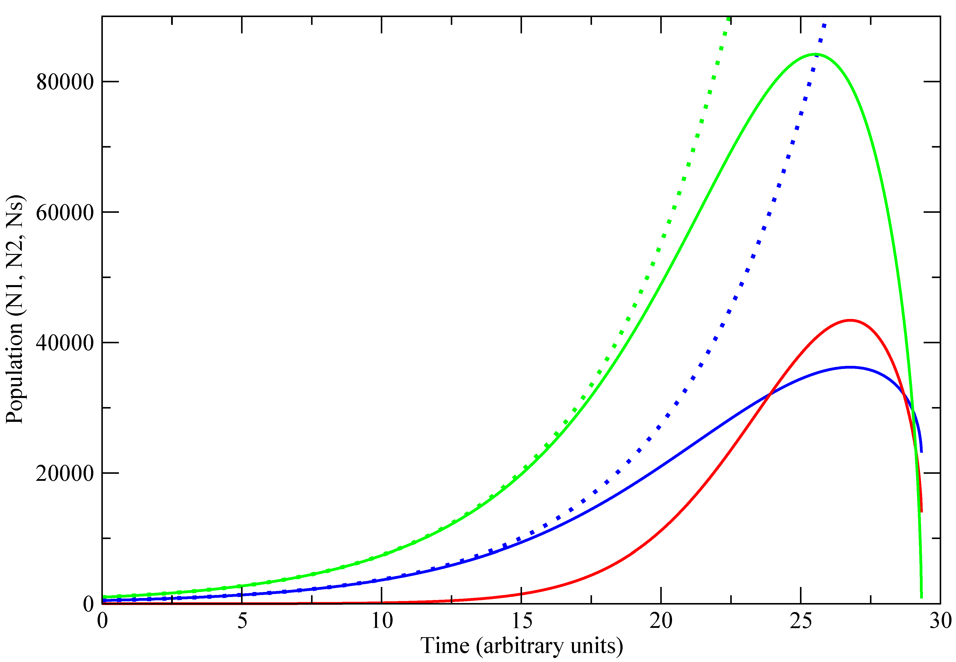
Figure 2. In the absence of competition, society 1 (blue) is in the exponential growth regime; its population growing more slowly than the carrying capacity. The introduction of the small but faster-growing society 2 has little effect initially (up to
); however, once it begins to grow, the total population approaches the carrying capacity, and around
the environment begins to deteriorate. Ultimately,
goes to zero, and both populations collapse; but this is not necessarily so. If neither population is susceptible to collapse, then collapse will not occur.
Figure 2.
Variation in population with time for a representative trajectory. , , , , , or 0. Blue lines represent population of society 1 (), Red line , Green lines . Solid lines are the competition case, dotted lines correspond to equivalent single population case . Since τ and G have scaled units, the absolute value of the population does not correspond to the number of individuals.
There are two implications to this. One is that any society will succumb to invasion by a faster-growing one (conquest). The ultimate collapse of Ancient Egypt can be assigned to this mechanism. It has been argued [
28] that the Roman culture brought high rates of birth and mortality (
), exactly the conditions required for a takeover followed by collapse of a previously slow-growing state. The second is that within a given society there is a selection bias in favour of any trend towards lower
τ. Thus even without external competition, evolution by natural selection drives a single isolated society toward instability.
2.3. Discussion
For the case of a single population with no spatial variation, we have shown that a coupling to the environment leads to a model with no stable state. We showed this explicitly for the simplest model, but it turns out to be true in all cases where the environment has no “self-healing” term, or where environmental improvement and degradation depend only on the current population.
We find that most scenarios give near-logistic growth followed by collapse. There is an exponential solution, based on innovation outstripping the population growth. However, this solution is evolutionarily unstable with respect to invasion by a faster-growing culture. Unfortunately, each successful invader brings the system closer to, or beyond, the unsustainable condition which leads to collapse. Once such a doomed invader appears, no stable culture can displace it, until it destroys the environment and collapses.
We have proved this result for a simple analytic case, but there is no respite in appealing to sociological “it’s more complicated than that” arguments. Introducing additional terms describing more complicated effects such as conflict or more-strongly nonlinear growth show the same behaviour. In this type of model, the only way that the expanding solution can be preserved is if the environment is self-repairing or not shared (i.e., is different for each population).
We prove in the
Appendix that analogous boom-bust dynamics occur for any alternate form where the rate of environmental modification depends only on the population—
i.e., whenever Equation (
2) is replaced by a function of
N only.
Our simple model casts into mathematical terms ideas such as those expressed in several books on societal collapse [
29,
30,
31,
32] and citations therein.
The brings us to the central question addressed by this paper. How could one obtain steady world population growth when our simple model of individual civilizations exhibits violent booms and busts? Two possible resolutions are presented in the next two sections.
3. Self-Repairing Environment
In some cases the environment may recover naturally. We can describe this behaviour by adding an extra term to Equation (
2), with a rate of recovery
b and a “natural” carrying capacity
to which the environment reverts in the absence of people:
Natural regeneration means that there is a stationary point at finite population
where
Consequently, for a stationary point to exist, must be positive. Thus stationary points exist whenever . When , a stationary point exists only for high enough b.
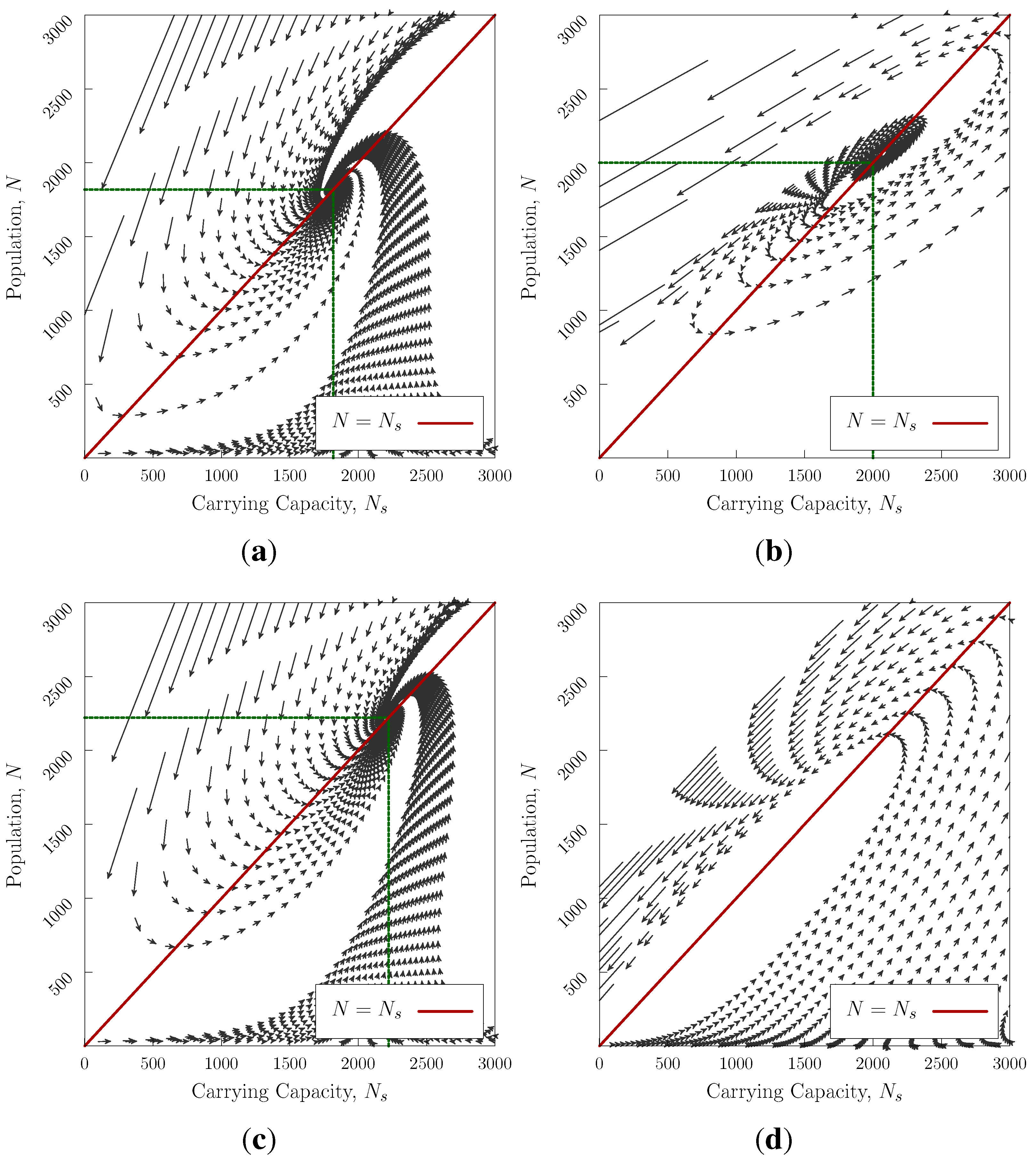
Figure 3 shows the evolution of the system for several values of
a,
b and
G. The stationary point may be either stable (an equilibrium point)
Figure 3a,c or unstable.
Figure 3b—it is notable that in the absence of a stationary point
Figure 3d the maximum pre-collapse population obtained is much higher than the other cases
Figure 3a–c. In two-civilisation competition (generalisation of Equation (
4)), the unstable case will win.
In the cases where a stationary point exists, we can linearise the system about
, finding two exponents (
, see
Appendix) which characterise the behaviour of fluctuations away from stationarity. For real, negative (positive)
λ, the system converges (or diverges) exponentially from the fixed point. For complex
λ the system spirals into (or away from) the equilibrium point. The stability criterion requires rapid natural regeneration compared with the difference in the rates of modification and population change
.
3.1. Effect of Noise
A final consideration is that the environment may be subject to random temporal fluctuations [
33]. We considered adding a stochastic term corresponding to a random walk of magnitude
σ
with
a gaussian random function with unit variance centred on 0. If the stationary point is unstable, the noise induces exponential growth away from it. If it is stable, the equilibrium is shifted slightly (see
Appendix), but the main effect is a stochastic resonance at the frequency defined by the imaginary part of
λ that drives the system out of equilibrium. While this is mathematically interesting, it probably has no actual ramifications. Once again, simulated results show that the general behaviour is unaffected by nonlinear terms.
Stable population size can be obtained if the environment can recover strongly. However, the stable population size is largely determined by the natural environment rather than the impact of population, representing a hunter-gatherer type population. A self repairing environment cannot explain the continuous growth exhibited by human history.
4. From Analytics to Computation: Variation in Space
We have shown that the standard logistic equation is unstable against coupling to the environment, and that non-collapsing strategies are uncompetitive compared with collapsing strategies. This may not be surprising; since most historical civilisations have undergone collapse, there is no conflict between model and data. However, the human population as a whole has increased, even as its various constituent civilisations disappear. Is there a way to achieve system-wide stability? A clue as to how this happens is contained in Equation (
4). It is the sharing of the environment which enables the fast-expanding population to exploit the innovations of their rivals: perhaps diversity and separation plays a role. We have previously seen that in a number of other complex evolving systems partial spatial separation confers stability [
34,
35].
Figure 3.
Trajectories in N vs approaching an equilibrium point for . Realistic scenarios would start at low N and always converge if equilibrium exists—initial conditions of high overpopulation may not be able to recover with passing into the negative region, which we interpret as societal collapse. (a) , , , and . Stable equilibrium point at ; (b) , , , and . Unstable stationary point at ; (c) , , , and . Stable equilibrium point at ; (d) , , , . No stationary point, system collapses.
The simplest reaction-diffusion equation which can give a travelling wave solution is the Fisher equation described in the introduction. It has been criticised as being based on diffusion; however, while it can be derived from a premise of random motion, the same mathematical form describes the situation where people migrate purposefully to more amenable areas. Thus, in a spatially-varying treatment, we add a spatial term which represents purposeful migration to regions of lower population or higher fertility [
18,
19], and yet simplifies to the diffusion equation for constant
.
So far we have concentrated on mathematically tractable analyses. We now turn to an algorithmic model with many populations dispersed in space and spatially-varying . This computational model is similar in conceptual simplicity to those above but with the added possibility of both applied and self-generated inhomogeneity in space and time. Each population is randomly assigned a relative birth rate (), innovation (), and aggression () factor (see below). To avoid the problem of simultaneously maximising all these characteristics, we have a constraint , representing the fraction of each population (or their time) dedicated to producing offspring, improving the environment, or fighting battles. New cultures are introduced at a random site by converting the population at this site and its neighbours to a different culture j with random .
The carrying capacity () of each site is also subject to diffusion, (constant ) as technology spreads from person to person, or as degradation spreads.
The complete algorithm can be summarised as:
- (1)
Update population due to a culture-specific birth rate () and a global natural death rate ();
- (2)
Convert people from one culture to another depending on the aggressiveness of each of the cultures;
- (3)
Population dynamics of each culture;
- (4)
Update the carrying capacity of each site based on the population weighted average of culture-specific modification;
- (5)
Mutate a random site at a random time by converting all of its inhabitants to a new randomly generated strategy ().
We have run simulations of the model with mobility and stochastic nucleation of cultures with characteristics drawn randomly from the range of plausible values [
36] (
7 km
year
;
0.1 year
;
0.01 year
;
0.02 year
);
1 year
A pattern appears that each culture emerges, spreads, and ultimately collapses either spontaneously or due to a faster expanding rival. A dynamic steady state is established with the total population growing fitfully over time.
Analytic solutions are now impossible, and the number of parameters in the model has become large. But the combination of the wave of advance [
10,
11] of a “superior” technology with the analyses given earlier enables us to understand what is going on. In a given location we observe a cycle of
Improvement of environment by innovators (high );
Invasion by a group, or groups, with higher , followed by collapse;
Inability of groups with negative environmental impact to occupy low region;
Improvement of environment by innovators (high ), cycle repeats.
Across the system as a whole, different regions are at different phases in the cycle, so the various strategies are always available to move into appropriate areas.
Certain strategies are more successful than others. Notably those with high innovation
(less aggressive, slower growing) tend not to be successful. While
is essential to maintain the quality of the land, such cultures are vulnerable to losing that territory to militaristic or fast-growing neighbours.
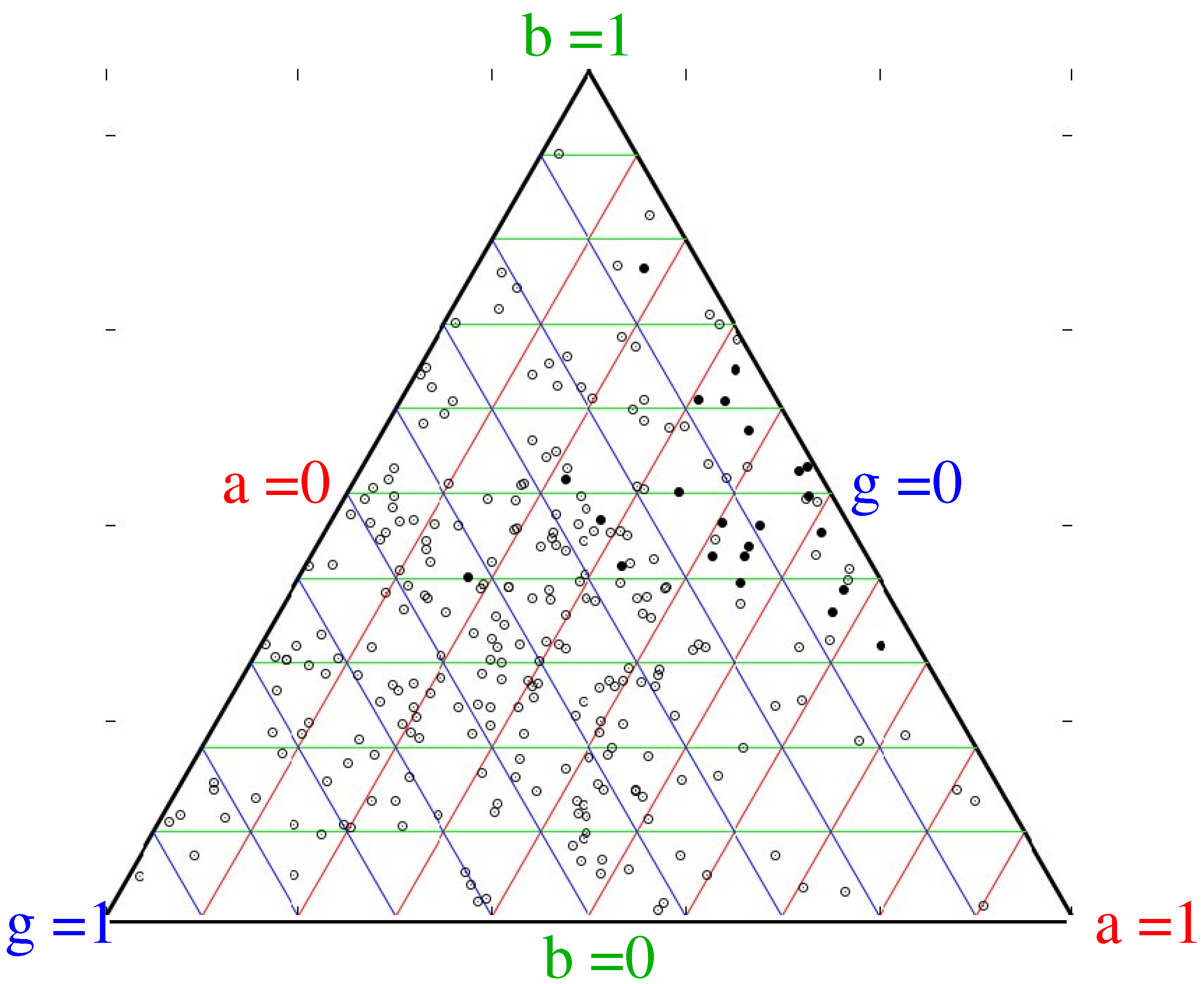
Figure 4 shows, for a range of simulations and initial conditions, which strategies can successfully invade: the most successful ones are those with a balance between high birthrate and high aggression, with consequently lower innovation.
Figure 4.
Typical graph showing strategies of randomly chosen successful (black) and failing (open) cultures. Each point on the figure represents a culture with a particular balance of , and b. The triangular form ensures that , with red, green and blue lines joining points of equal a, b and g respectively. Aggression ranges from on the left line to at the right apex, Modification ranges from on the right line to at the left apex, Birthrate ranges from on the bottom line to at the top apex, A “successful” culture is defined as a mutation which grows to become, at some point, the largest in the simulation. This is one of many runs, but all show the same pattern that the successful invaders have low modification and balanced aggression and birthrate.
There are two limiting cases for the system, and curiously neither is stable. If the diffusion constant is set to zero, successful cultures cannot spread and eventually an environment-destroying collapse occurs at each site (
c.f. Figure 1). Less obviously, if the diffusion constant is very high we reach a globalisation state where one strategy dominates throughout, and all the regions are in the same phase in the cycle described above. Now, when the collapse comes, it is truly global and the entire system is depopulated.
A final limiting case is to allow “diffusion” of environment —this represents the idea that an while an improvement such as an irrigation canal cannot itself diffuse, the idea of an irrigation canal can. The outcome of this is, once again, globalisation and the collapse of the entire system once an overpopulating society takes hold. Remarkably, this is true even if environmental diffusion is set up so that only positive effects are adopted: is always increased by diffusion (i.e., at each site is either increased towards the mean of the adjacent site, or held constant at each timestep: Max[]). History suggests that the value of , the sharing of expertise and technology, is continually increasing. If this is the case, then the unpalatable outcome of such sharing is that an unstable level of globalisation will ultimately occur.
5. Conclusions
We have developed a model for population dynamics in the presence of coupling to the environment based on simple, intuitive concepts. We have been unable to find a simple model which gives a static solution of sustainable population, or a long-term supraexponential growth which recent human history actually exhibits. Indeed all models have solutions which either involve expansion and collapse, or predict exponential growth but are susceptible to invasion by ultimately-doomed strategies.
If the environment can self-repair, a stable strategy can be found at a population only weakly dependent on innovation, and close to the natural “carrying capacity”. Unfortunately, such a strategy is evolutionarily unstable against a faster growing but ultimately collapsing strategy.
We have examined analytically solvable models, and shown by computation that more complex, nonlinear models give similar outcomes. We therefore believe that our results are robust against additional perturbations. These results are consistent with the actual history of individual human civilisations.
Long-term system-wide stability can be obtained by introducing spatial variation in the model, with many cultures with different strategies in competition. Provided the extremes of localisation and globalisation are avoided, spatial effects provide the stable growth of the system viewed as a whole, which typifies human history. It appears that, once environmental coupling is considered, the continued existence of humanity is possible only via the continual rise and fall of civilisations. Even this is ultimately unstable if technology is widely shared across a globally homogeneous civilisation.
