The Supply and Demand Mechanism of Electric Power Retailers and Cellular Networks Based on Matching Theory

Department of Electronic and Communication Engineering, North China Electric Power University, Baoding 071003, China
*
Author to whom correspondence should be addressed.
Information 2018, 9(8), 192; https://doi.org/10.3390/info9080192
Submission received: 25 June 2018
/
Revised: 17 July 2018
/
Accepted: 19 July 2018
/
Published: 27 July 2018
(This article belongs to the Section Information and Communications Technology)
Abstract
:With the rapid increase of wireless network traffic, the energy consumption of mobile network operators (MNOs) continues to increase, and the electricity bill has become an important part of the operating expenses of MNOs. The power grid as the power supplier of cellular networks is also developing rapidly. In this paper, we design two levels of bilateral matching algorithm to solve the energy management of micro-grid connected cellular networks. There are multiple retailers (sellers) and clusters (buyers) in our system model, which determine the transaction price and trading energy respectively and have a certain influence on the balance of energy supply and demand. Retailers make more profits by adjusting the price of electricity in matching algorithm M-1, depending on the energy they capture and the level of storage. At the same time, clusters adjust the electricity consumption through matching algorithm M-2 and power allocation on the basis of ensuring the quality of users’ service. Finally, the performance of the proposed scheme is evaluated by changing various parameters in the simulation.
1. Introduction
In recent years, the prelude of a new round of the energy revolution has commenced, since the distributed energy resources, which have the properties of low environmental costs, renewability, and world-wide distribution, have been increasingly integrated into the power system [1,2,3]. Traditional power systems will face a significant transition to cope with the new changes and challenges. In view of this, micro-grids that are comprised of networked groups of distributed loads and renewable generators become an appealing solution. Micro-grids have the characteristics of flexible location and decentralization, which is well adapted to the distributed power demands and resource distribution, so that the reliability of power supply can be improved effectively. Furthermore, it is very important to coordinate the energy management of power generation and electricity consumption in the micro-grid. On the other hand, cellular networks as power users are consuming more and more energy. The cellular network can flexibly adjust the electricity consumption according to its own demands and external environment, which makes the cellular network play a very important role in the micro-grid. Therefore, energy management will be a fundamental challenge in micro-grid connected cellular networks.
A micro-grid is a small decentralized independent system, which can realize self-control, protection and management of autonomous systems. It can be connected to the grid or run in isolation. Micro-grids may transform between these two modes because of scheduled maintenance, degraded power quality or a shortage in the host grid, faults in the local power grid, or for economic reasons [4,5]. The micro grid works in island mode if it has enough local supply from the renewable farm; otherwise, it connects to the main grid to purchase on-grid energy [6]. When the micro grid is connected to the power grid, it can play the role of peak load shaving in the large power grid, which is a strong support for the stable operation of the large power grid. When the power grid fails, the micro grid can be separated quickly from the big power grid and operates independently, providing continuous power supply for the government, hospitals and transportation hubs, and improving the reliability of the power supply. By means of modifying energy flow through micro-grid components, micro-grids facilitate the integration of renewable energy generation, such as photovoltaic, wind and fuel cell generation, without requiring re-design of the local power grid system [5,7,8]. Modern optimization methods can also be incorporated into the micro-grid energy management system to improve efficiency and flexibility [8]. The micro-grid not only solves the large-scale access problem of distributed power supply, but also takes the advantages of distributed power supply and brings other benefits to users. Micro-grids will fundamentally change the traditional way of coping with load growth, and have great potential in reducing energy consumption and improving the reliability and flexibility of power system.
With the rapid increase of wireless network traffic, the energy consumption of mobile network operators (MNOs) continues to rise and the electricity bill has become an important part of operating expenses of MNOs. Based on the characteristics of a cellular network, it can reduce the energy consumption flexibly by regulating their own traffic. Therefore, a cellular network can play a certain role in energy management of a micro-grid. The work in [9] considers that the base stations are aggregated as a micro grid with hybrid energy supplies and an associated central energy storage, which can store the harvested renewable energy and the purchased on-grid energy over time to minimize the on-grid energy cost of a large-scale green cellular network. A novel architecture for micro-grid connected cellular networks is proposed in [10], which are equipped with renewable energy generators and finite battery storage to minimize energy cost. In fact, base stations can reduce energy consumption through business cooperation or energy cooperation. The resource and traffic can be reasonably allocated among the base stations through coordinated multiple points (CoMP), which can always guarantee the minimum overall transmit power consumption while meeting the throughput requirement of each user (UE) and also each base station (BS)’s power constraint [11,12,13]. In practice, there may be multiple MNOs at the same time, and they are cooperative or non-cooperative [14,15]. In the literature [14,15], each MNO reduces the energy cost by sharing energy and management strategies between them, and also reduce the energy cost of the network through batteries and renewable energy harvesting devices. In this paper, MNOs are treated as independent power users in the micro-grid, and their own strategy is to maximize their own benefits.
In a smart grid, the power grid allows two-way power flow and the distributed renewable energy generators as the sellers in the micro grid can supply the captured energy to users or the power grid. In the literature [16,17], the electricity retailers as the leaders in the Stackelberg game sell energy to a cellular network, meanwhile multiple clusters in the cellular network adjust the energy consumption with sleep mode. Wu et al. [18] investigates a hybrid energy trading market that is comprised of an external utility company and a local trading market managed by a local trading center with its own electricity price. In this paper, the retailers optimize their strategy through the electricity price, determine whom to sell and how much electricity they sell, and store the remaining electricity in storage for future use.
In this paper, we propose an optimized energy management framework for micro-grid connected cellular networks. In the micro-grid involving multiple retailers and clusters, the buyers (clusters) and sellers (retailers) make strategies and influence each other, determine the transaction price and trading energy, and have a certain influence on the balance of energy supply and demand. Each cluster can adjust the energy consumption flexibly and also ensure the quality of service (QoS). According to the different price of electricity and the level of traffic, MNOs can adjust the electricity consumption on the basis of ensuring the quality of uses’ service. At the same time, retailers make more profits by adjusting the price of electricity, depending on the energy they capture and the level of charge they can store.
Furthermore, we not only consider the energy demand of clusters, but also consider the electricity price strategy of retailers. The operation of the cellular network depends on the price, channel condition and service requirement of the users. The clusters decide on which retailers to procure electricity from and how much electricity to procure, considering the price of each retailer. We design two levels of bilateral matching model: the first is the matching M-1 between the retailers and the clusters, and the other is the matching M-2 between the base stations and the users. We utilized the distributed matching algorithms as the solution to the above problem.
The rest of this paper is organized as follows: Section 2 presents the system model and energy consumption of BS. Section 3 presents problem formulation. In Section 4, we propose distributed matching algorithms. Simulation results are analyzed in Section 5. Finally, conclusions are drawn in Section 6.
2. The System Model and Energy Consumption of BS
2.1. The System Model
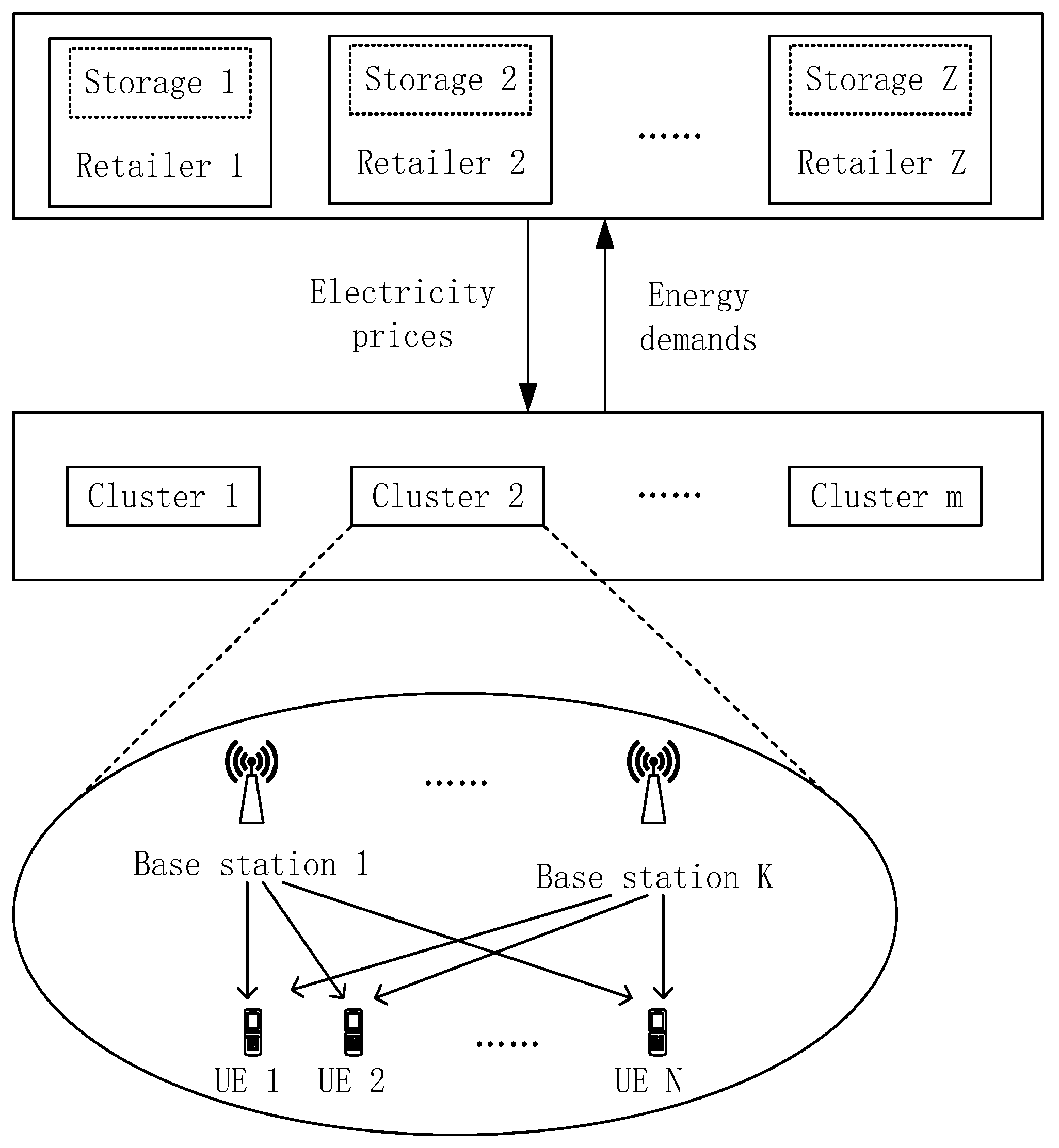
We assume that there is a wireless cellular network comprised of M clusters denoted as and powered by Z retailers denoted as , as shown in Figure 1. We assume that each cluster belongs to different MNO, so we denote the th BS and the th UE in mth cluster by and , respectively. We assume that each retailer is equipped with energy generators and a storage device. In the system model, we only consider the optimization problem in one time slot, so we define the amount of power captured by the retailer in this time slot as . We assume that the maximum capacity of the storage is denoted by and the amount of energy stored at this time slot is denoted by BEz. In the paper, each cluster has K base stations denoted by serving N users denoted by . For convenience, we define the index sets , , , and . Each UE is required to associate with base station and each cluster needs to buy electricity from the retailers to meet the user’s service requirement.
2.2. The Energy Consumption of BS
In the system, cellular networks purchase electricity from retailers to service users. Each cluster needs to consider both the traffic needs of users and the electricity price provided by the retailers to tradeoff between throughput benefit and energy cost. The energy consumption model for the cluster is described below.
We assume that each cluster has K base stations denoted by serving N users denoted by . The energy demand of the cluster is the total energy consumption of the base stations in it. The power consumption of a base station is divided into two parts: static energy consumption and dynamic energy consumption. Static energy consumption refers to the power consumption of a base station without any traffic load. Dynamic energy consumption refers to the additional power consumption caused by the traffic load on the BS. Suppose that the dynamic energy consumption is zero when the base station has no traffic. The energy consumption function of the kth base station is as follows:
where denotes the static energy consumption of BS according to the different type of base station and usually is set to a constant, denotes the weight ratio of the dynamic energy consumption of BS, denotes the dynamic energy consumption of the kth BS. is a matching parameter, when denotes that the user n is served by the jth sub-channels of base station k, otherwise . represents the transmit power of the base station k to serve user n. The relationship between the matching parameters of the BSs and the user with the transmission power can be denoted as follows:
When the dynamic energy consumption of BS is zero, the total traffic load of BS is zero, indicating that there is no user needs service.
3. Problem Formulation
In this paper, the system model has three layers, which are the retailer layer, the cluster layer, and the user layer. Two bilateral-matchings are used in the whole system model, which are the matching (M-1) between the power retailers and the clusters, the matching (M-2) between the base stations and the users in the cluster.
In the system model, the retailers provide power or energy to the clusters as the commodity in the electricity market. For convenience, each time slot is normalized to unity unless otherwise specified, thus the terms “energy” and “power” will be used interchangeably in the sequel [19]. In the side of selling energy, retailers make a profit by selling as much electricity as possible at higher prices than its cost price, and retailers can’t sell more than the sum of the energy they capture and the energy stored in their storage. When the matching process ends, if the remaining energy of the retailer is more than the capacity of storage, retailers will sell the remaining energy to the main grid at cost price, so that there will be no profit loss. In the side purchasing energy, the clusters can allocate resources reasonably to users to improve the throughput of the whole cluster through matching algorithm and power allocation, which can reduce the purchase cost while satisfying the quality of service. In order to better study the strategy changes of retailers’ price and clusters’ energy demand, we consider one-to-many matching model, where each retailer sells electricity to multiple clusters while each cluster only purchases electricity from one cluster. In the matching process, sellers (retailers) and buyers (clusters) optimize their utility and influence each other through the energy price and the energy demand as the decision variable, respectively. In the paper, the matching (M-1) between the retailers and clusters and the matching (M-2) between the BSs and users are used to optimize the utility of each individual participating in the system (e.g., increasing the profit of power retailers and reducing the energy cost of clusters). The next section will formulate two matching issues and give their constraints.
The proposed algorithms are based on matching theory. To model the competitive behavior of UEs, BSs, clusters and retailers, we first define their utility functions.
3.1. The Matching (M-1) between Retailers and Clusters
In this section, we formulate the matching algorithm M-1 to solve the system’s utility optimization problem. We first define retailers’ and clusters’ utility functions as follows. The increase of the demand for energy from the clusters will result in the increase of the retailer’s profit, so one of the most common criteria for retailers to select clusters is to consider the power demand of the cluster. The utility of retailer z when it is connected to cluster m can be written as
Then we define the utility function of retailer m as the sum of the electric profit of , as follows:
where is the component of matrix , which indicates if and are matched or not, denotes the amount of power purchased by cluster m at retailer z, denotes the price of the retailer z selling electricity to clusters, denotes the cost of the retailer z selling electricity to clusters.
In the process of matching, the cluster is expected to increase the transmission rate as much as possible while reducing the purchase cost. Therefore, the utility of the cluster is divided into two parts. We define the utility of cluster m when it is connected to retailer z can be written as:
Then the utility of cluster m can be written as follows:
where denotes the total throughput of cluster m, is the positive real number, which is to unify the units of the two parts of throughput and energy cost. denotes the amount of power purchased by cluster m at retailer z. represents the cost of the cluster m purchasing power.
In M-1, each retailer can sell electricity to multiple clusters, but cannot exceed the maximum amount of electricity sold, so the utility function and constraints of retailers can be written as:
where is the matrix comprising of elements . Constraint (a) states that retailer z can sell of electricity at most. Constraint (b) guarantees that each cluster will be matched with only one retailer and constraint (c) states that the values of can be only 0 and 1.
Each cluster can only buy electricity from one retailer, so the utility function and constraints of clusters can be written as:
In the process of solving the problem (7), the retailers adjust the price according to matching algorithm (M-1), then the energy demand and utility of clusters are obtained through matching algorithm (M-2) and power allocation. In the next section, we’ll give you a detailed description of the sub-matching algorithm (M-2))
3.2. The Matching (M-2) between Base Stations and Users
In the algorithm mentioned above, the power demand of each cluster is obtained through the following matching algorithm (M-2). At the first, we discuss the matching algorithm between the base stations and the users in a single cluster.
We use a three-dimensional pairing matrix , where each element is a binary variable to represent the set of resource allocation strategies. For example, denotes that user n is established between BS k and sub-channel j. Accordingly, the binary decision variables and the continuous power variables should be jointly designed to optimize the system performance. The problem of matching M-2 is formulated as:
Constraint (a) states each UE will be matched with only one BS and sub-channel, constraint (b) states that a maximum of UEs can be matched with each BS and constraint (c) states that a maximum of UEs can be matched with each sub-channel. Constraint (d) states that the values of can be only 0 or 1.
3.3. Power Allocation
After the matching algorithm M-2 allocates the user to the appropriate base station and sub-channel, the optimal power allocation can be formulated as:
Condition (a) guarantees that the sum of the allocated powers to each base station is not more than the maximum transmission power , condition (b) guarantees that each user’s transmission rate is not lower than .
4. Distributed Matching Algorithm
In the process of bilateral matching, in order to make each agent satisfied with the matching object, the matching tendency can be ranked from high to low by preference list, and finally get the optimal utility of the agent. In the whole matching algorithm, M-1 and M-2 algorithms solve the problem through the following steps. In the M-1 algorithm, first all retailers announce the electricity price to clusters. After that, the distribution of resources and the demand energy in the cluster are calculated by M-2 matching algorithm based on the electricity price and channel conditions. Each cluster establishes a preference list for retailers and applies to the first retailer in the list. Then retailers decide which clusters to match and update the electricity price by comparing the energy demand of clusters that apply to match with the maximum energy available for sale. The above is an iterative process. Each iteration in the matching process will update the electricity price of retailers and the energy demand of the clusters. Specific steps for the M-1 and M-2 algorithms are explained in the following sections.
In this section, we propose distributed matching algorithms to solve the problems formulated in Section 3. We use the following two matching algorithms, M-1 and M-2 algorithms, to solve the matching problems M-1 and M-2, respectively. From Definition 1, we define matching functions and for the M-1 and M-2, respectively, where , and are the maximum number that can be matched. and are the price allocation matrices corresponding to functions and , respectively.
4.1. The Matching (M-1) between Retailers and Clusters
In M-1 we propose a bilateral matching algorithm where both retailers and clusters selfishly and rationally interact to maximize individual utility function. Retailers increase their profits by changing the price of electricity. At the beginning of M-1 matching algorithm, the price of the retailer’s electricity will be set as its cost price. In the matching process, the retailer z will raise the price of electricity by step-number and then sell energy to the cluster if the amount of power exceeds the maximum that can sell. Clusters will adjust the demand of electricity according to channel state and the price of the retailers, then reduce the cost of purchasing electricity and increase the rate through M-2 and power allocation. The aim of the M-1 is to optimally solve the optimization problem in (7) through matching algorithm between the retailers sets with the serving clusters . The specific details of the algorithm are described in Algorithm 1, with the notations defined below.
First, will announce the price of unit electricity to the cluster according to its cost price. Then, will form a descending preference list in terms of its utility over all the potentially available retailers, that is, the first retailer in is obtained from the following formula (M-1-Step 1)
Thus, such that if and only if .
To summarize the M-1, to increase the throughput and reduce the cost of electricity, each cluster first chooses the best retailer and bids for it (M-1-Step 2-1). We will define a bid function as
has a descending ordered list of the clusters that bid for . The list is ordered based on the received utility, that is, the first in corresponds to , (FM-1-Step 2-1).
Thus, such that if and only if . In M-1-Step 3, retailers will decide if they want to match with the clusters that bid for them. There are three possibilities. The first possibility (M-1-Step 3-1) is that receives no bids from clusters after increasing its price-allocation number, but in the previous iteration, had received bids from multiple clusters. will choose these clusters which could maximize the utility of to be matched with. The second possibility is that has bid from multiple clusters (M-1-Step 3-2-a). will increase its price allocation number by for the next (gen+1)st iteration. Note that represents the price-step number, which indicates the price-allocation number offered from the clusters to the source increases at each step. The third possibility (M-1-Step 3-2-b) is that has received a bid from only one cluster. In this case, will be matched with this one. The last iteration of the M-1 is denoted as tEnd.
| Algorithm 1 The bilaterally matching algorithm between the retailers and the clusters. |
| Step 1: Initialization (1) Set , , , . (2) Set . (3) Construct the list of all the clusters that are not matched, , and preference list to all the retailers denoted by , . Step 2: Clusters’ Demand of Power (1) Each announces its price-allocation number to all the unmatched clusters . (2) For all (a) If , then
(3) Construct the descending ordered list of clusters that bided for in terms of utility, . (4) Tag the clusters in by index t as Step 3: Retailers’ Decision Making (1) For all (a) If , then
(2) Set . (3) If is not empty go to Step 2; otherwise, go to step 4. Step 4: End of the Algorithm |
To study the stability of the matching problem between retailers and clusters, we adopt the following theorem used in the assignment game problem in [19] and adapt it to our two-sided matching algorithm:
Theorem 1.
The algorithm in Algorithm 1 produces matching and price-allocation matrices, which are in competitive equilibrium for sufficiently small values of δ.
The proof of Theorem 1 is similar as that in the literature [19], which is omitted there.
4.2. The Matching (M-2) between Base Stations and Users
We propose a matching approach to solve the mixed integer programming problem (9). In our system, we attempt to solve the problem (9) by employing the three-dimensional matching that user equipment, base stations and sub-channels with each other. To reduce the computational complexity, we transform the original three-dimensional matching to a two-sided matching. First, we define a BS-SUB unit, which is composed of one base station and one sub-channel (SUB). Owing to the existence of K BSs and J SUBs, there are K × J different BS-SUB units, denoted by . Thus, the three-dimensional matching problem can be simplified to a two-sided matching with N UEs on one side and K × J BS-SUB units on the other side.
The distributed algorithm which solves the optimization problem (9) involves each UE and BS-SUB strategically maximizing their utility functions. From Section 2, we know that the static power consumption of the base stations in the cluster is constant. Therefore, in the setting of utility function (13), we’re going to make an analogy to the utility of the user to the function of the cluster. Users’ utility value is also divided into two parts: throughput benefit and energy consumption. At the same time, in order to better allocate resources to users, BS-SUB takes the channel condition between the user applying for it and BS-SUB as its utility. Compared with the utility of all users that apply to match, BS-SUB allocates its own resources to the best user and matches it.
The utility functions of UEs’ and BS-SUBs’ are respectively expressed as follows:
After obtaining the price of electricity published by retailers, the dependent variables of clusters’ utility are channel conditions and power allocation. In order to better analyze the effect of these two dependent variables on cluster utility, we divided the resource allocation problem into two sub-problems: M-2 matching and power allocation. In order to distinguish between channel state and power distribution in the utility function, we do not consider the effects of the distribution of power in the matching algorithm (M-2). We know that in the same power allocation, the user will transmit at a higher rate with better channel conditions, so they will be inclined to choose the BS-SUB unit with better channel state to match. In order to simplify the complexity of the matching process, we denote the function of the user’s preference for BS-SUBs as:
Then UE will establish the preferences list for BS-SUB based on this function.
The aim of the M-2 is to optimally solve the optimization problem in Equation (9) through matching the UEs sets with the serving BS-SUBs , while maximizing the sum rates of all the UEs in the cluster. The specific details of the algorithm are described in Algorithm 2, with the notations defined below.
First, will form a descending order preference list in terms of its utility over all the potentially available BS-SUB, i.e., the first BS-SUB in corresponds to . Thus, such that if and only if .
To summarize the M-2, each UE first chooses the best BS-SUB and bids for its (FM-2-Step 2-1). We will define a bid function as:
has a descending ordered list of the UEs that bid for . The list is ordered based on the received utility, that is, the first UE in corresponds to (FM-2-Step 2-1). Thus, such that if and only if .
Because each BS-SUB can serve at most one user, we can make the following two cases in M-2-Step 3. The first possibility (M-2-Step 3-1-a) is that is not matched with the user, and then selects the highest utility value user match in the iteration and rejects the rest users. The second possibility (M-2-Step 3-1-b) is that the has already matched user n and it will compare the current matching user with the user who is applying for the iteration, and selects the user with the highest utility value. If the user has no higher utility value than the current matched user, the current matching result is retained. Otherwise, replace it and reject the remaining users.
In M-2-Step 4, BSs and SUBs will decide if they want to match with the UEs that bid for them respectively. There are two possibilities. The first possibility (M-2-Step 4-1-a) is that the receives more than bids from UEs. will choose select the top users in the bid list and reject the remaining UEs. The second possibility (M-2-Step 4-1-b) is that the receives applications less than . In this case, will be matched directly with this UE. SUBs can also get results in the same way. Then we will end the bilaterally matching algorithm until is empty.
| Algorithm 2 The bilaterally matching algorithm between BS-SUBs and UEs. |
Step 1: Initialization
For all
(1) For all (a) If , then
(i) . (ii) Set and remove from . (2) . (3) If is not empty go to Step 2; otherwise, go to step 4. Step 4: BSs’ and subs’ Decision Making (1) For all (a) If , then
(a) If , then
(4) If is not empty go to Step 2; otherwise, go to step 5. Step 5: End of the Algorithm |
In order to study the stability of Algorithm 2 proposed by matching theory, first, we adopt the following concept used in the so-called college admissions problem in [20] and adapt it to our matching approach:
Definition 1.
An assignment of BS-SUBs to users will be called unstable if there are two BS-SUBs α and β which are assigned to users A and B, respectively, although β prefers A to B and A prefers β to α.
In the proposed approach, the users bid to the first BS-SUBs of their preference list. Each BS-SUB is allocated to the user with the higher preference, that is, the user with the larger value. If α is assigned to A rather than B, A has a higher preference value on α when compared to B. Similar reasoning can be made for user B and BS-SUB β. Then certainly, A prefers α to β; otherwise user A would be allocated subcarrier β and not α. If α is allocated to A instead of B, then the value of A is higher than B over BS-SUB α. Thus, the assignment that is performed in our proposed algorithm abides by the preferences of the users and BS-SUBs, and therefore it is a stable assignment. The assignment is stable at each iteration of the algorithm. In fact, after utility evaluation, the preference list of each user is updated and the matching routine is repeated, each time resulting in a stable assignment.
We refer to the analysis of the stability of three-dimensional matching in literature [21], and finally reach the following conclusions: the matching process would end with finite iterations; the proposed Algorithm 2 can converge to a two-sided stable matching in finite iterations; and the solution of three-dimensional matching is weak Pareto optimal for users on combinations of base stations and sub-channels.
4.3. Power Allocation
After the result of matching algorithm M-2 is obtained, each user will allocate the optimal power in order to maximize its own utility. The optimal power allocation problem (10) can be solved by referring to the Lagrange dual algorithm similarly in literature [19] and the optimal power can be obtained.
5. Simulation Results
In this section, we provide simulation results to validate our theoretical analysis and evaluate the performance of the proposed scheme. According to Section 4, clusters derive the optimal solution based on reasonable resource allocation to decide how much electricity is procured from the retailer. Retailers also derive the optimal solution to decide the electricity price. To evaluate the performance of the proposed algorithms, we consider there are three retailers denoted by which provide energy to six different clusters denoted by . We set the maximum capacity of each storage is , only for the traffic of the clusters is low in our setting. In the simulation, is randomly distributed between 0 and 2000 mW and retailers to capture for 300~500 mW in the time slot. The retailers’ cost price and initial electricity price are and , respectively, where the price unit is normalized without loss of generality [20]. There are 4 base stations and 32 users, which are randomly deployed in each cluster with a cell radius of 300 m. We set the path loss exponent to 4 and the thermal noise level to −110 dBm. We assume the maximum transmission power of the base station as 200 mW and the minimum transmission rate of the user as 200 kbit/s. Finally, we set and the number of sub-channels is 8.
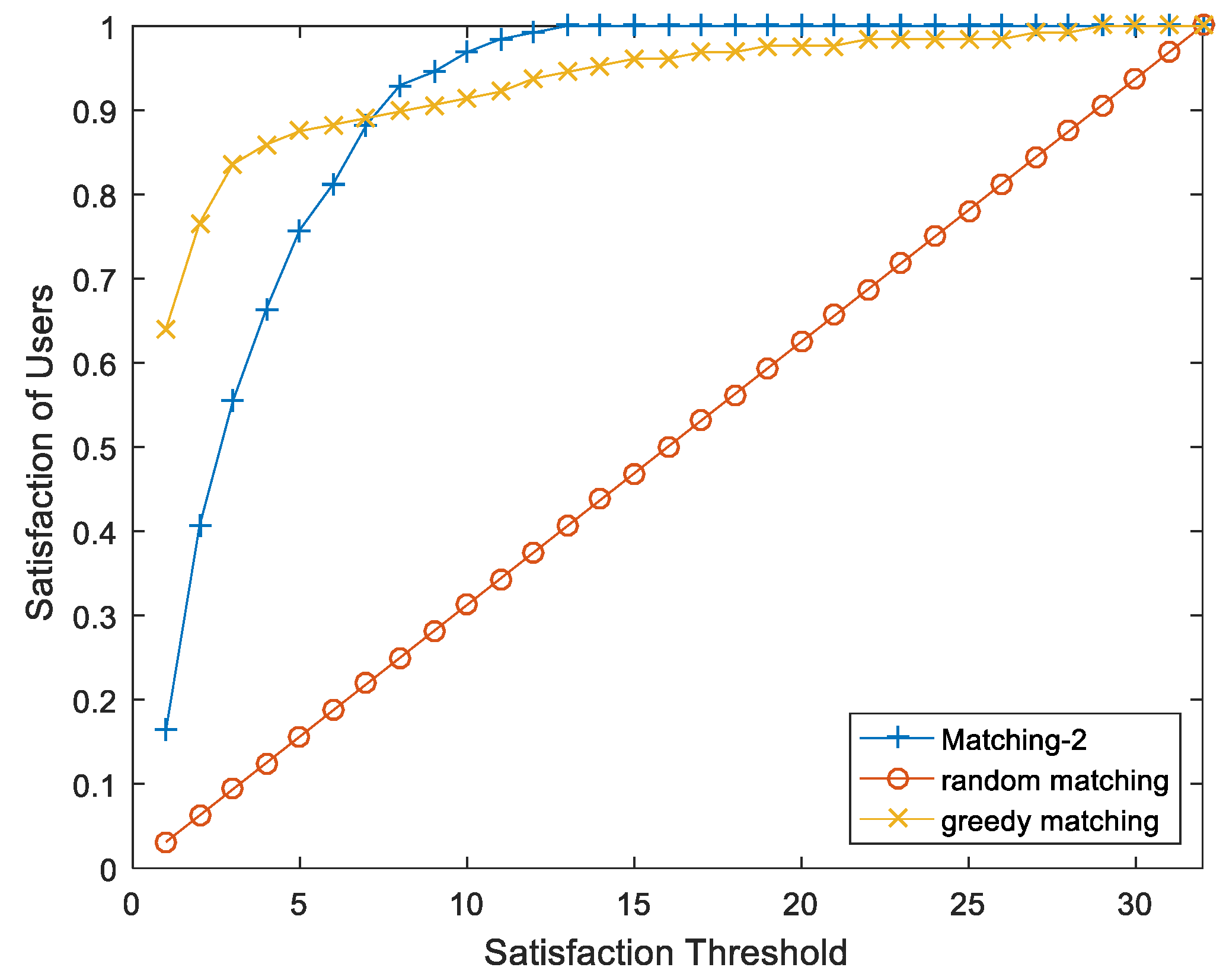
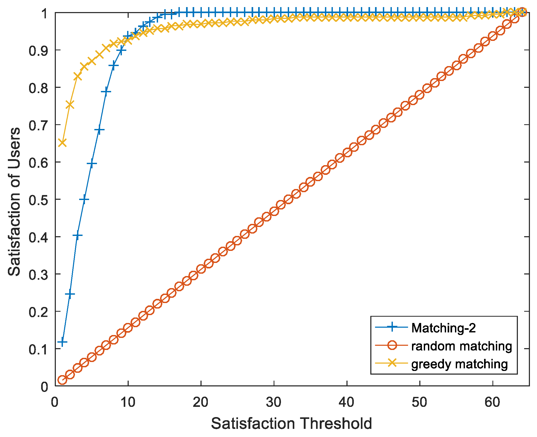
Figure 2 and Figure 3 show the users’ satisfactions versus various satisfaction thresholds with N = 32, K = 4, J = 8 and N = 64, K = 8, J = 8. We obtain the numerical results of Figure 2 and Figure 3 by averaging the results of 100 times running the simulation. In the case of N = 32, K = 4, J = 8, the probability of being matched to the first three choices for users under M-2 is 55.47% and the probability of being matched to the first ten choices for users is as high as 94.53%. In contrast, the corresponding probability under random matching is only 9.38% and 31.25%. In the case of N = 64, K = 8, J = 8, there is 40.23% and 93.75% of users that have been matched to the first three and ten choices, respectively. At the same time, the corresponding probability under random matching is decreased to only 4.69% and 15.63%. We can see that the matching M-2 algorithm can achieve significant satisfaction gains compared to the random matching.
In Figure 2 and Figure 3, we can see that users in the greedy matching algorithm only choose the best BS-SUB, so the user satisfaction of the greedy matching algorithm is higher than the M-2 algorithm in the first few options. However, the M-2 algorithm is more concerned with the overall resource allocation of the cluster, which can reach 100% user satisfaction in the first 20 choices or even the first 15 choices. Therefore, the M-2 algorithm is superior to greedy matching algorithm in the overall performance of the cluster.
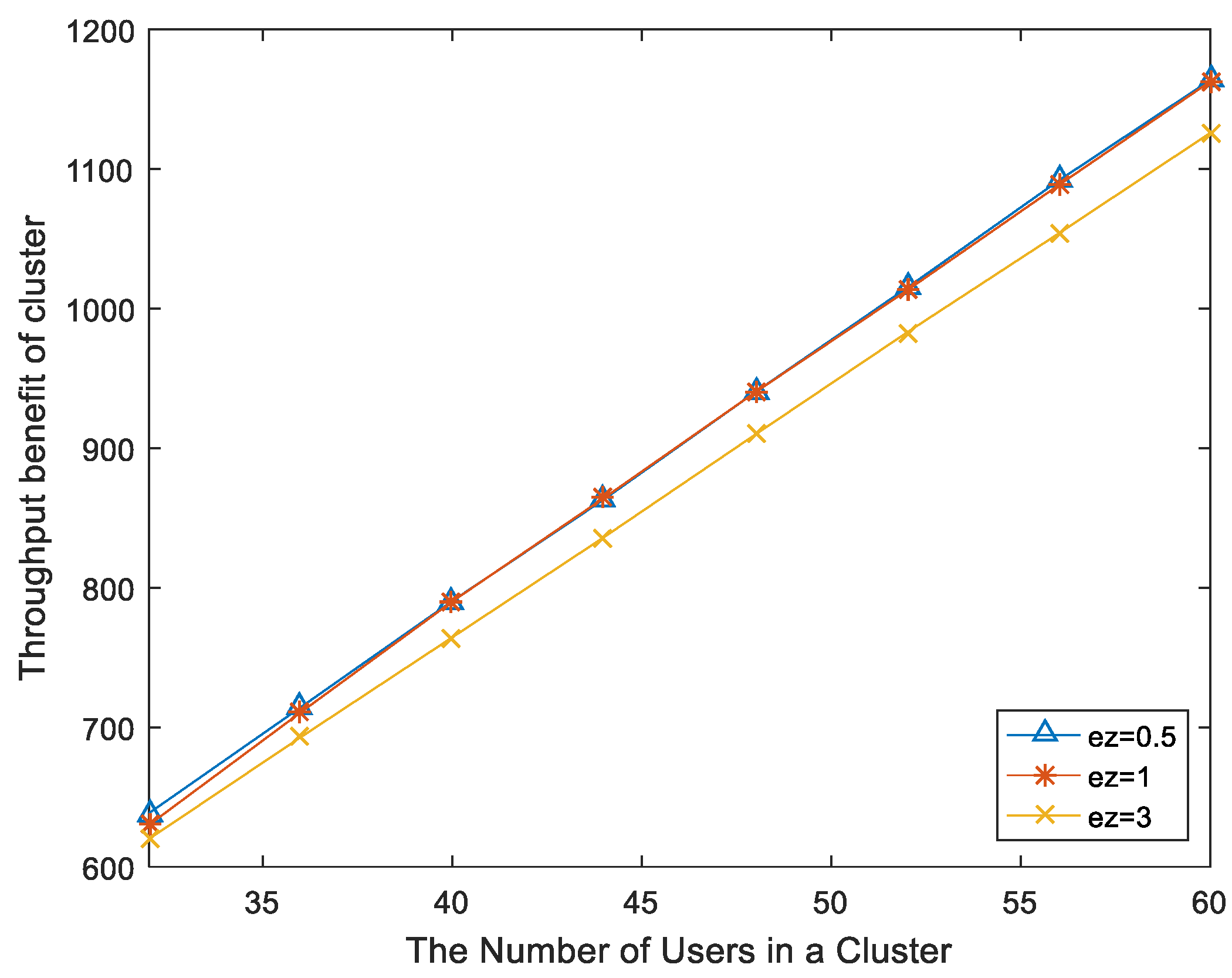
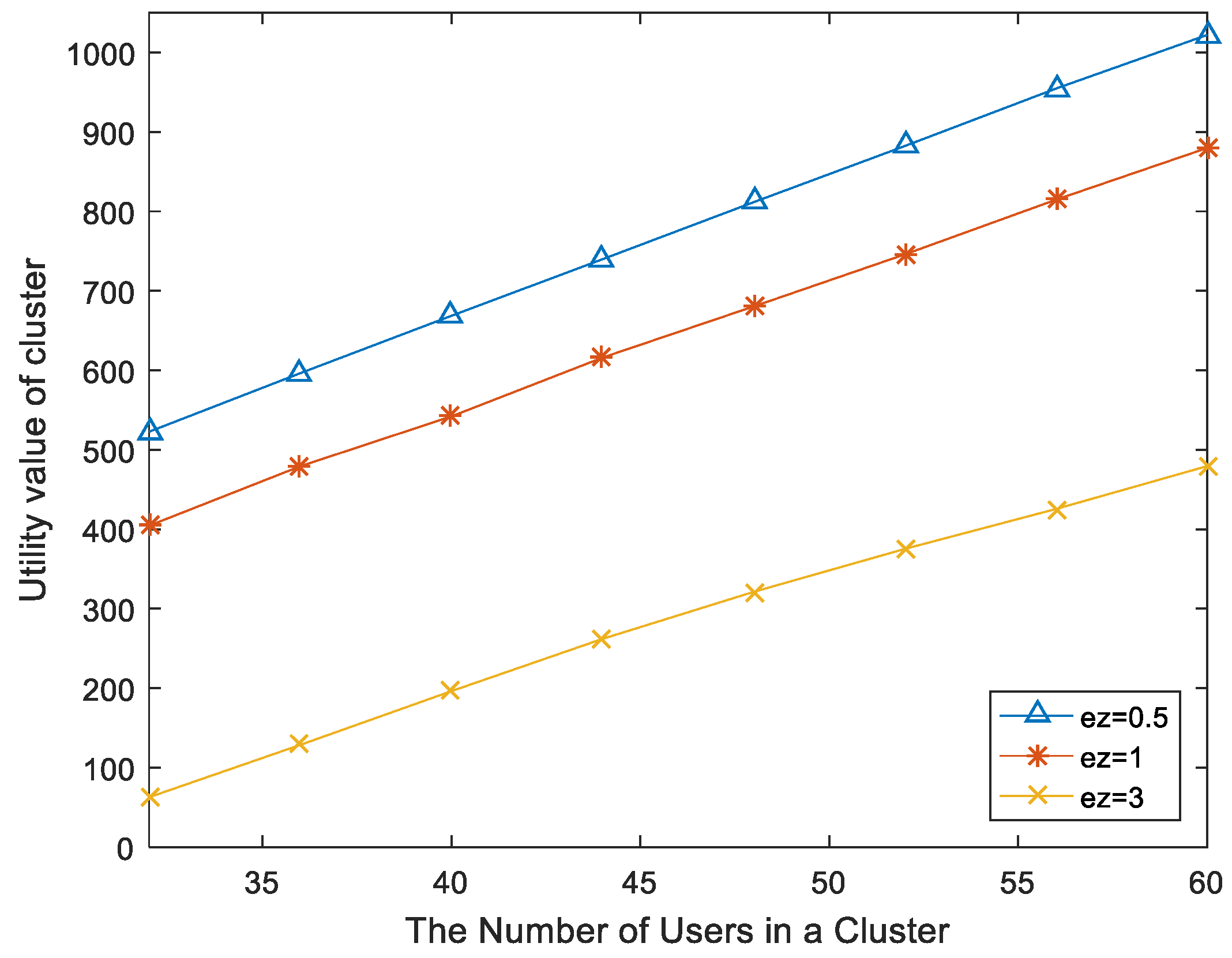
Figure 4, Figure 5 and Figure 6 show the variation trends of throughput benefit, energy consumption and utility value of a cluster versus the number of users in a cluster, respectively. At the same time, we calculate these three values according to three different electricity prices ez. As we can see from the Figure 4, Figure 5 and Figure 6, the increase in the number of users in a cluster will result in a significant increase in the throughput benefit of the cluster, and electricity consumption will also rise. However, the optimal power allocation algorithm can smooth the growth trend of energy consumption due to its negative utility in the cluster. Therefore, we conclude that the increase of the number of users in a cluster will lead to the increase of the utility value of the cluster. When the number of users in a cluster increased from 32 to 60, the energy consumption of the cluster increased by 22.32%, 25.43% and 16.01% and the utility value of the cluster increased by 499, 475 and 416 under different electricity prices (ez = 0.5; ez = 1; ez = 3). At the same time, the throughput benefit of the cluster is not very different, while the energy consumption increases but does not show a multiple relationship. In the case of N = 32, ez = 0.5 as the reference group, we can know that the energy consumption of ez = 1 and ez = 3 are 1.948 and 4.81 times of the reference group, respectively. From Figure 6, we can see that the utility value of the cluster decreases as the price of electricity rises, and the trend of utility value changes with the price of electricity is analyzed in Figure 7.
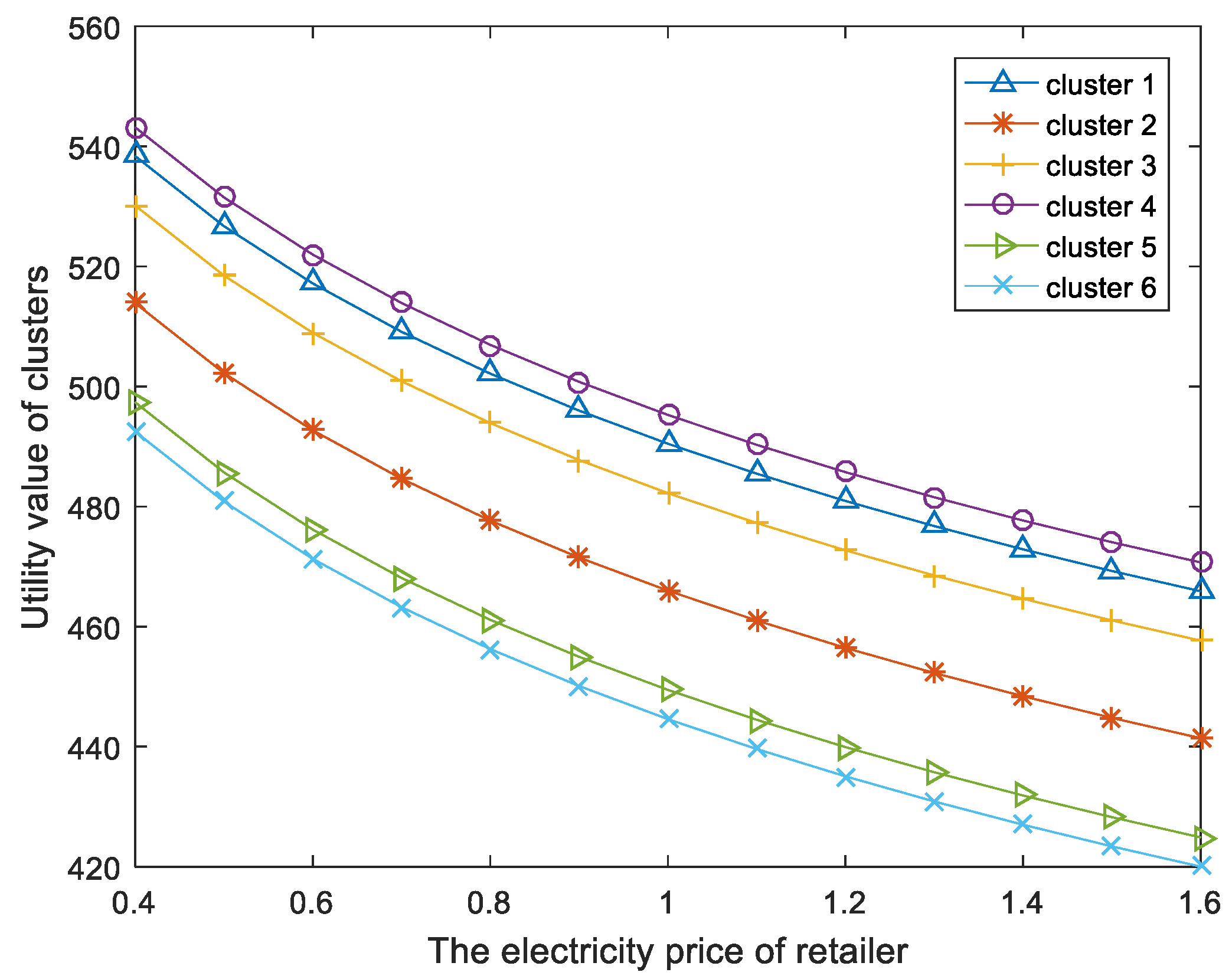
In Figure 7 we can see that the utility value of each cluster is gradually decreasing when the electricity price of the retailer increases. The clusters will weaken the growth trend of energy demand when the price of electricity rises, but cannot effectively reduce the impact of the increase of electricity price on the continuous increase of electricity consumption.
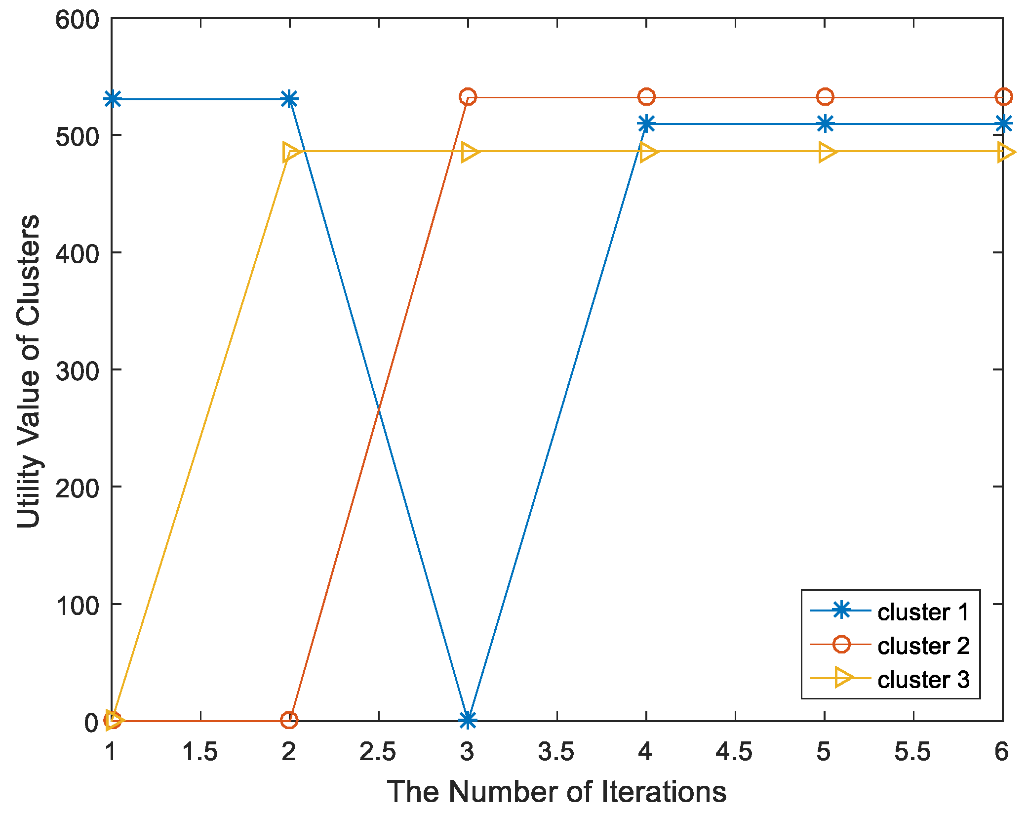
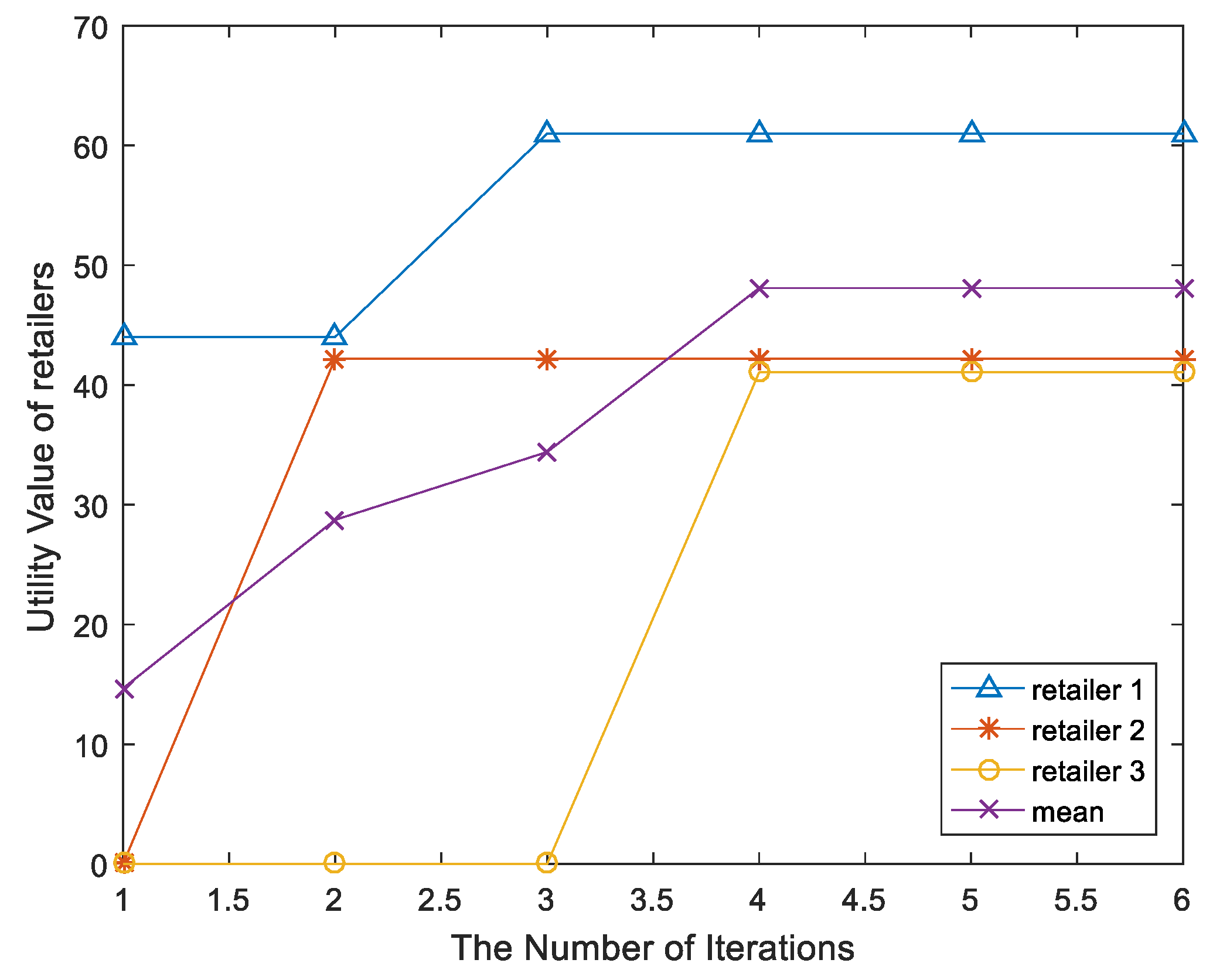
Figure 8 and Figure 9 show the change of utility value of cluster and retailer with the number of iterations. We set the electricity price of three retailers as ez1 = 0.4, ez2 = 0.5, ez3 = 0.6, and the price step-number as δ = 0.1. In Figure 8, we select three typical clusters to analyze the change trend of utility value with the number of iterations. Initially, each cluster will buy as much electricity as possible at the lowest price, and then the rejected cluster reduces utility (because the electricity price of retailer is higher) by buying electricity from another retailer. In the process of matching, the retailer will reject the existing matching cluster if the retailer is asked to match by the cluster with a higher profit, so the retailer’s utility value will gradually increase in the matching process and finally converge to stable matching. In fact, if the number of retailers increases, the cluster becomes more optional and the utility value will increase as competition decreases, and vice versa.
6. Conclusions
This paper considers the energy management of a micro-grid connected cellular network, involving multiple retailers and clusters. The simulation results show that the M-2 matching algorithm can significantly improve user satisfaction, and the cluster utility increases with the increasing number of users in the cluster, and decreases as the electricity price of the retailers increases. At the same time, the retailer’s profits will gradually increase in the process of the M-1 algorithm and finally converge to stable matching. If the number of retailers increases, the cluster has more options and the retailer’s utility decreases with less competition between the clusters, and vice versa. Optimizing resource allocation for clusters with multiple time slots in a multi-retailer energy supply scenario could be an interesting future topic.
Author Contributions
W.H. proposed the idea and wrote this paper; W.H. and Y.K. conceived and carried out the simulation; W.H. and B.L. analyzed the data; all authors have read and approved the final manuscript.
Funding
The work in this paper was supported in part by the National Natural Science Foundation of China (Grants No. 61501185), and the Hebei Province Natural Science Foundation (Grants No. F2016502062), and the Fundamental Research Funds for the Central Universities (2016MS97), and the Beijing Natural Science Foundation (Grants No. 4164101).
Conflicts of Interest
The authors declare no conflict of interest.
References
- Katiraei, F.; Iravani, M.R. Power Management Strategies for a Microgrid with Multiple Distributed Generation Units. IEEE Trans. Power Syst. 2006, 21, 1821–1831. [Google Scholar] [CrossRef]
- Parhizi, S.; Lotfi, H.; Khodaei, A.; Bahramirad, S. State of the Art in Research on Microgrids: A Review. IEEE Access 2015, 3, 890–925. [Google Scholar] [CrossRef]
- Liu, S.; Liu, P.X.; Wang, X. Stochastic Small-Signal Stability Analysis of Grid-Connected Photovoltaic Systems. IEEE Trans. Ind. Electron. 2016, 63, 1027–1038. [Google Scholar] [CrossRef]
- Olivares, D.E.; Mehrizi-Sani, A.; Etemadi, A.H.; Canizares, C.A.; Iravani, R.; Kazerani, M. Trends in Microgrid Control. IEEE Trans. Smart Grid 2014, 5, 1905–1919. [Google Scholar] [CrossRef]
- Salam, A.A.; Mohamed, A.; Hannan, M.A. Technical Challenges on Microgrids. J. Eng. Appl. Sci. 2008, 3, 64–69. [Google Scholar]
- Fang, X.; Misra, S.; Xue, G.; Yang, D. Smart Grid—The New and Improved Power Grid: A Survey. IEEE Commun. Surv. Tutor. 2012, 14, 944–980. [Google Scholar] [CrossRef]
- Kanellos, F.D.; Tsouchnikas, A.I.; Hatziargyriou, N.D. Micro-Grid Simulation during Grid-Connected and Islanded Modes of Operation. In Proceedings of the 2005 International Conference on Power Systems Transients (IPST 05), Montreal, QC, Canada, 19–23 June 2005. [Google Scholar]
- Jin, M.; Feng, W.; Liu, P.; Marnay, C.; Spanos, C. MOD-DR: Microgrid Optimal Dispatch with Demand Response. Appl. Energy 2017, 187, 758–776. [Google Scholar] [CrossRef]
- Che, Y.L.; Duan, L.; Zhang, R. Dynamic Base Station Operation in Large-Scale Green Cellular Networks. IEEE J. Sel. Areas Commun. 2016, 34, 3127–3141. [Google Scholar] [CrossRef] [Green Version]
- Farooq, M.J.; Ghazzai, H.; Kadri, A.; Elsawy, H.; Alouini, M.S. Energy Sharing Framework for Microgrid-Powered Cellular Base Stations. In Proceedings of the 2016 IEEE Global Communications Conference (GLOBECOM), Washington, DC, USA, 4–8 December 2016. [Google Scholar]
- Huang, X.; Ansari, N. Joint Spectrum and Power Allocation for Multi-Node Cooperative Wireless Systems. IEEE Trans. Mob. Comput. 2015, 14, 2034–2044. [Google Scholar] [CrossRef]
- Chia, Y.; Sun, S.; Zhang, R. Energy Cooperation in Cellular Networks with Renewable Powered Base Stations. IEEE Trans. Wirel. Commun. 2013, 13, 6996–7010. [Google Scholar] [CrossRef]
- Xu, J.; Zhang, R. Cooperative Energy Trading in CoMP Systems Powered by Smart Grids. IEEE Trans. Veh. Technol. 2016, 65, 2142–2153. [Google Scholar] [CrossRef]
- Leithon, J.; Lim, T.J.; Sun, S. Energy Exchange among Base Stations in a Cellular Network through the Smart Grid. In Proceedings of the 2014 IEEE International Conference on Communications (ICC), Sydney, Australia, 10–14 June 2014; pp. 4036–4041. [Google Scholar]
- Farooq, M.J.; Ghazzai, H.; Kadri, A.; Elsawy, H.; Alouini, M.S. A Hybrid Energy Sharing Framework for Green Cellular Networks. IEEE Trans. Commun. 2017, 65, 918–934. [Google Scholar] [CrossRef] [Green Version]
- Bu, S.; Yu, F.R.; Cai, Y.; Liu, X.P. When the Smart Grid Meets Energy-Efficient Communications: Green Wireless Cellular Networks Powered by the Smart Grid. IEEE Trans. Wirel. Commun. 2012, 11, 3014–3024. [Google Scholar] [CrossRef]
- Bu, S.; Yu, F.R. Green Cognitive Mobile Networks with Small Cells for Multimedia Communications in the Smart Grid Environment. IEEE Trans. Veh. Technol. 2014, 63, 2115–2126. [Google Scholar] [CrossRef]
- Wu, Y.; Tan, X.; Qian, L.; Tsang, D.H.K.; Song, W.Z.; Yu, L. Optimal Pricing and Energy Scheduling for Hybrid Energy Trading Market in Future Smart Grid. IEEE Trans. Ind. Inf. 2017, 11, 1585–1596. [Google Scholar] [CrossRef]
- Bayat, S.; Li, Y.; Song, L.; Han, Z. Matching Theory: Applications in Wireless Communications. IEEE Signal Process. Mag. 2016, 33, 103–122. [Google Scholar] [CrossRef]
- Gale, D. College Admission and the Stability of Marriage. Am. Math. Mon. 1962, 69, 9–14. [Google Scholar] [CrossRef]
- Xu, C.; Feng, J.; Huang, B.; Zhou, Z.; Mumtaz, S.; Rodriguez, J. Joint Relay Selection and Resource Allocation for Energy-Efficient D2d Cooperative Communications Using Matching Theory. Appl. Sci. 2017, 7, 491. [Google Scholar] [CrossRef]
Figure 1.
The system model.

Figure 2.
Users’ satisfactions versus satisfaction threshold (n = 32, K = 4, J = 8).

Figure 3.
Users’ satisfactions versus satisfaction threshold (n = 64, K = 8, J = 8).

Figure 4.
Throughput of cluster versus the number of user in a cluster (K = 8, J = 8).

Figure 5.
Energy consumption of cluster versus the number of user in a cluster (K = 8, J = 8).
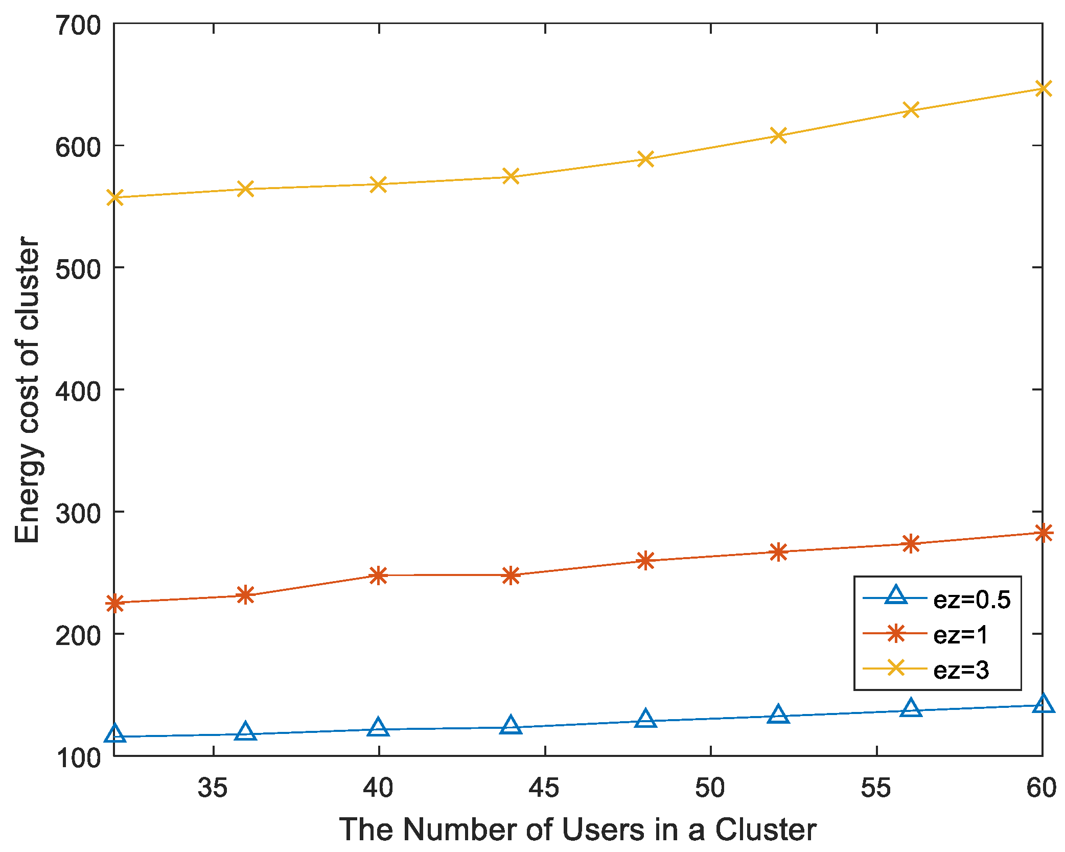
Figure 6.
Utility value of cluster versus the number of user in a cluster (K = 8, J = 8).

Figure 7.
Utility value of cluster versus the electricity price of the retailer (N = 32, K = 8, J = 8).
Figure 7.
Utility value of cluster versus the electricity price of the retailer (N = 32, K = 8, J = 8).

Figure 8.
Utility value of cluster versus the number of iterations (N = 32, K = 8, J = 8).

Figure 9.
Utility value of retailer versus the number of iterations (N = 32, K = 8, J = 8).
© 2018 by the authors. Licensee MDPI, Basel, Switzerland. This article is an open access article distributed under the terms and conditions of the Creative Commons Attribution (CC BY) license (http://creativecommons.org/licenses/by/4.0/).
Share and Cite
MDPI and ACS Style
Kong, Y.; Huang, W.; Li, B. The Supply and Demand Mechanism of Electric Power Retailers and Cellular Networks Based on Matching Theory. Information 2018, 9, 192. https://doi.org/10.3390/info9080192
AMA Style
Kong Y, Huang W, Li B. The Supply and Demand Mechanism of Electric Power Retailers and Cellular Networks Based on Matching Theory. Information. 2018; 9(8):192. https://doi.org/10.3390/info9080192
Chicago/Turabian StyleKong, Yinghui, Wenchan Huang, and Baogang Li. 2018. "The Supply and Demand Mechanism of Electric Power Retailers and Cellular Networks Based on Matching Theory" Information 9, no. 8: 192. https://doi.org/10.3390/info9080192
Note that from the first issue of 2016, this journal uses article numbers instead of page numbers. See further details here.