Target Tracking Algorithm Based on an Adaptive Feature and Particle Filter


1
College of Engineering, Huaqiao University, Quanzhou 362021, China
2
University Engineering Research Center of Fujian Province Industrial Intelligent Technology and Systems, Huaqiao University, Quanzhou 362021, China
*
Author to whom correspondence should be addressed.
Information 2018, 9(6), 140; https://doi.org/10.3390/info9060140
Submission received: 10 May 2018
/
Revised: 6 June 2018
/
Accepted: 7 June 2018
/
Published: 8 June 2018
(This article belongs to the Section Information Processes)
Abstract
:To boost the robustness of the traditional particle-filter-based tracking algorithm under complex scenes and to tackle the drift problem that is caused by the fast moving target, an improved particle-filter-based tracking algorithm is proposed. Firstly, all of the particles are divided into two parts and put separately. The number of particles that are put for the first time is large enough to ensure that the number of the particles that can cover the target is as many as possible, and then the second part of the particles are put at the location of the particle with the highest similarity to the template in the particles that are first put, to improve the tracking accuracy. Secondly, in order to obtain a sparser solution, a novel minimization model for an Lp tracker is proposed. Finally, an adaptive multi-feature fusion strategy is proposed, to deal with more complex scenes. The experimental results demonstrate that the proposed algorithm can not only improve the tracking robustness, but can also enhance the tracking accuracy in the case of complex scenes. In addition, our tracker can get better accuracy and robustness than several state-of-the-art trackers.
1. Introduction
Target tracking has always been a popular research direction in the field of computer vision as it has important applications in scene monitoring, behavior analysis, autopilot, robot, and so forth [1,2,3]. Although the visual tracking technology has made considerable progress, and a large number of excellent tracking algorithms have been proposed [4,5,6,7,8,9,10,11], there are still a series of unpredictable challenges, such as occlusion, motion blur, pose and shape change, illumination change, scale variation, and so on. Therefore, developing a robust tracking algorithm has always been a very tough task.
The particle-filter-based tracking algorithm has attracted a great number of scholars’ attention because it has the advantages of simple implementation, parallel structure, and strong practicality, etc. Inspired by Yang [11], certain relationships between the particles could be exploited through the lower rank and the temporal consistency. However, the low rank and the temporal consistency cannot exploit the relationship between the particles when the scene changes greatly between two adjacent frames or the distribution of the particles of the current frame is relatively dispersed. Therefore, a relatively simple and effective approach for exploiting the relationship between the particles is proposed. Compared with all of the particles that are put at once in each frame in the traditional particle-filter-based tracking algorithms, in our tracking algorithm, all of the particles are divided into two parts and are put separately in each frame. Through the intelligent cooperation between the two parts of the particles, the number of particles that cover the target increases, which can improve the tracking accuracy.
Chartrand [12] first proposed the Lp norm, and it has proved to be more excellent than the L1 norm [13,14]. Many problems, based on sparse coding for image restoration and image classification, are solved with the non-convex Lp norm minimization model. Compared with solving the L1 norm minimization model, solving the Lp minimization model can usually gain sparser and more accurate solutions. Considering this advantage, the Lp norm is applied so as to solve the sparse representation coefficients, and a novel minimization model for an Lp tracker is proposed to improve the tracking accuracy in this paper.
Combining multiple observation views has proven to be beneficial for tracking. The tracking algorithm is difficult to adapt to some complex scenes when using only a single feature to represent the target. Considering that a feature generally only adapts to a certain type of scene, the advantage of the complementary features can be used, that is, by combining multiple features to represent the target, in order to improve the robustness of the tracking algorithm to complex scenes. Hong et al. [15] proposed a multi-task multi-view tracking algorithm (MTMVT). Four complementary features, including color histograms, intensity, histogram of oriented gradient (HOG), and local binary pattern (LBP), were used to represent the target, which could overcome the influence of complex scenes, to some extent. Inspired by MTMVT, we propose a novel multi-feature fusion strategy with adaptive weights, which can adaptively adjust the weights of different features according to the current scene, to determine the state of the target.
This paper is organized as follows. In Section 2, the materials and methods are summarized. In Section 3, we introduced the particle filter framework and sparse representation. Section 4 presents the details of the proposed algorithm, including the intelligent particle filter, the minimization model for Lp tracker, and the adaptive multi-feature fusion strategy. The experiments are conducted to compare with several state-of-the-art trackers in Section 5. Finally, we summarized this paper in Section 6.
2. Materials and Methods
According to the different expression strategies that have been adopted by the appearance models, the tracking algorithms could be generally divided into two categories, generative and discriminative approaches. Among them, the generative approach was used to establish a descriptive model in order to represent the target, and to then use it to search for the most similar region as the target in the image [16]. Because the proposed tracking algorithm belonged to the generative approach, we have focused on some related works of the generative approach.
The theory of sparse representation has been widely used in the target tracking algorithms [4,5,6,7,8]. Mei et al. [6] combined sparse representation with a L1 norm minimization model to improve the particle-filter-based tracking algorithm, which obtained good tracking results. However, the L1 norm minimization model needed to be solved for each particle at each frame, which led to a high computational complexity of the algorithm. To enhance the tracking speed, Mei et al. [7] proposed a minimum boundary error rule to remove some insignificant particles, which could reduce the number of calculating L1 norm minimization model. To improve the tracking speed and accuracy at the same time, Bao et al. [8] improved the algorithms that were proposed by the authors of [6,7], through adding the L2 regularization term on the coefficients that were associated with the trivial templates in the L1 norm minimization model, and used the accelerated proximal gradient (APG) method to accelerate the speed of solving sparse coefficients. Zhang et al. [17] imposed a weighted least squares technique, which could release the sparsity constraint on the traditional sparse representation methods to achieve strong robustness against appearance variations, and that utilized structurally random projection to reduce the dimensionality of the feature, while improving computational efficiency. Meshgi et al. [18] proposed an occlusion-aware particle filter framework by utilizing a binary flag to attach to each particle, in order to estimate the occlusion state according to the state and to treat occlusions in a probabilistic manner.
In recent years, the Lp norm was widely used. Zhang et al. [19] proposed an Lp norm relaxation to improve the sparsity exploitation of the total generalized variation. Xie et al. [20] generalized the nuclear norm minimization to the Schatten Lp norm minimization, which achievedd good results both in background subtraction and image denoising. Wang et al. [21] proposed to impose a L2,p norm regularization on self-representation coefficients for an unsupervised feature selection. Chartrand [22] developed a new non-convex approach for matrix optimization problems, involving sparsity to the decomposition of video into low rank and sparse components, which could separate moving objects from the stationary background better than in the convex case.
Using the advantages of multiple features to improve the tracking robustness was a popular approach. Hong et al. [15] represented the target by using four complementary features to overcome the problem of complex scenes, yet they did not highlight which feature was more important in some scenes. Dash et al. [23] utilized texture feature and Ohta color features in the feature vector of the covariance tracking algorithm, which was capable of handling occlusion, camera motion, appearance change, and illumination change, nevertheless the algorithm had a poor tracking performance for targets with insignificant color features. Yoon et al. [24] proposed a novel visual tracking framework that fused multiple trackers with different feature descriptors in order to cope with motion blur, illumination changes, pose variations, and occlusions, but every tracker used a single feature and ignored other features. Morenonoguer et al. [25] developed a robust tracking system by applying the appearance and geometric features to segment a target from its background, and showed impressive result on the challenges, but the tracking system had a poor real-time performance. Yin et al. [26] combined color information, motion information, and edge information in the framework of particle filtering to solve the problem of illumination variation and similarly colored background clutters, but the tracking performance of the algorithm was not stable when the background was complicated, and the contrast between the target and the background was low. Zhao et al. [27] fused the color feature and the Haar feature to overcome the challenges of illumination and pose change, but the algorithm could not handle partial occlusion. Tian [28] represented the target by the multiple feature descriptions, based on the selected color subspace, to improve the robustness of the target tracking to some extent. However, the algorithm was not able to handle the occlusion trouble.
Based on the ideas of the above literature, we employed a particle filter as a tracking framework and made use of the properties of the Lp norm, and then a tracking algorithm based on the Lp norm and the intelligent particle filter (Lp-IPFT) was proposed. In addition, on the basis of the Lp-IPFT, combined with the advantages of the multiple features, an adaptive multi-feature Lp-IPFT (AMFLp-IPFT) was proposed.
3. Introduction to the Related Theory
3.1. Particle Filter Framework
The particle filter transforms target tracking into a problem of estimating the target state through the known target measurement information. It calculates the posterior probability by two steps of prediction and update, supposing that represents the target state (the location and the shape of the target) in the t-th frame, and represents the target observations from the first frame to the t-th frame. According to the maximal approximate posterior probability, the optimal state of the target can be obtained in the t-th frame, as follows:
where represents the state of the i-th particle in the t-th frame. In the particle-filter-based tracking algorithm, the expression of the prediction and the update equation are as follows:
where represents the observation likelihood between the target state and the observed state , which is inversely proportional to the reconstruction error of the particle, see Equation (8). denotes the state transition model, which uses six independent parameters of the affine transformation to represent the target state , where represent the x translation, y translation, rotation angle, scale, aspect ratio, and skew direction, respectively. In general, the state transition model can be described by a zero-mean Gaussian distribution with diagonal covariance, as follows:
where and denote the variance of the above six independent parameters, respectively.
Applying the method mentioned above, according to the particle state , the candidate particles can be obtained in the t-th frame, as follows:
where denotes real number, represents the number of rows of the candidate particle , and represents the number of the candidate particles.
3.2. Sparse Representation
The sparse representation model is mainly utilized to calculate the observation likelihood of the sample state , which reflects the similarity between the candidate particle and the target template. Assuming that the target template set of the t-th frame is , and the corresponding candidate particle set is in the t-th frame, then the sparse representation model is as follows:
where is a trivial template set, and are the sparse coefficients of the target templates and the trivial templates, respectively, so is sparse. In addition, to ensure that the L1 tracking algorithm has a better robustness, it needs to impose nonnegative constrains on . Then, the sparse representation of can be obtained by solving Equation (7), as follows:
where . Finally, the observation likelihood of can be given by the following expression:
where is a constant for controlling the shape of the Gaussian kernel, is a standard factor, and is the minimizer of Equation (7), restricted to .
4. The Proposed Tracker
To improve the tracking accuracy and robustness, we propose three improvements on the basis of the L1-APG proposed by Bao et al. [8] as follows: (1) intelligent particle filter; (2) the minimization model for Lp tracker; and (3) an adaptive multi-feature fusion strategy. With these improvements, the proposed algorithm can not only take advantage of the robustness to occlusion from sparse representation, but it can also introduce complementary features’ representation for appearance modeling.
4.1. Intelligent Particle Filter
The traditional particle-filter-based tracking algorithms directly put all of the particles in accordance with the Gaussian distribution, according to the state of the particles in the previous frame, and do not take into account the relationship between these particles. When tracking a fast moving target, the tracking accuracy is affected because of the small or even zero number of particles covering the target. To tackle this problem, in our tracking algorithm, all of the particles are divided into two parts. In the first part, the particles are put in the same way as the traditional particle filter, while the other particles are put at the location where the particle that is put in the first part is most similar to the target template. Figure 1 illustrates the details of the particles put in the third frame of the Deer sequence.
As we know, the more that particles cover the target, the more accurate the tracking result are. Assuming that the total number of particles is , the number of particles in the first part is , the number of particles in the other part is , and >> . If , taking into account the computational complexity of the algorithm, the total number of particles is usually not too large, then the number of particles in the first part will be too small to cover the target, which is difficult for ensuring that the first part of the particles can provide effective information for the second part of particles, and then the function of the second part of the particles will be completely lost. Aiming at the problem, namely that it is difficult for the particles to cover the target, one common solution is to increase the number of particles, and the other common solution is to modify the affine parameters so as to make the particles more dispersed to enlarge the covering area. For the latter solution, since the distribution of the particles is too scattered, and the interval between the particles becomes larger and the reliability of the particles becomes smaller, it is easy to provide the wrong information for the second part of particles. Therefore, for the first part of the particles, we have employed the first solution, that is, increasing the number of particles in the first part to ensure that as many particles as possible can cover the target, so we choose .
In this paper, the particles are divided into two parts. The second part of the particles are put at the location where the particle is most similar to the target template in the first part, which is equivalent to putting the second part of the particles at or around the candidate target. This can improve the tracking accuracy. It can be said that the second part of the particles play a supporting role in the tracking process, its effect is equivalent to slightly adjusting the state (including the location, rotation, scale, and so on) of the optimal particles (candidate target) in the first part, to improve the tracking accuracy and robustness. At the same time, taking the relationship between the two parts of the particles into consideration, the affine parameters of the particles in the second part are smaller than that of the particles in the first part. Therefore, compared with the traditional particle filter, we have taken full account of the relationship between the particles. Our particles are intelligent, and they (the first part of the particles and the second part of the particles) can effectively assist, thus improving the tracking accuracy and robustness.
4.2. The Minimization Model for Lp Tracker
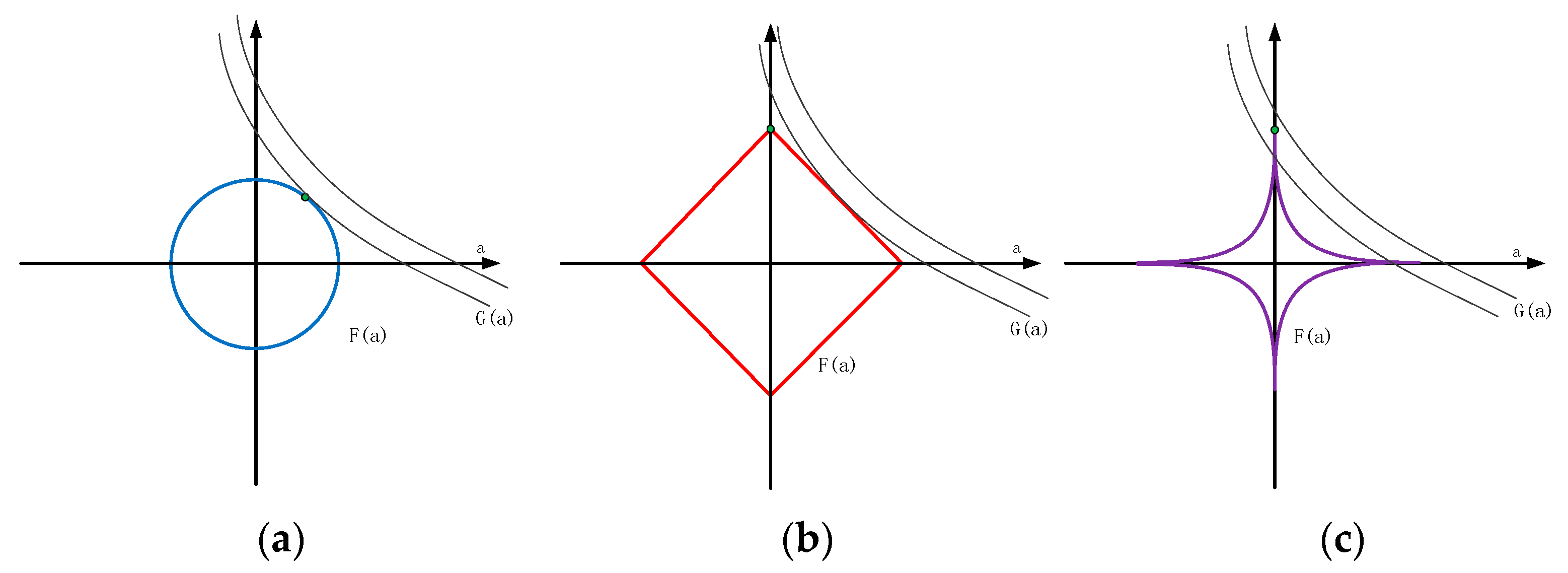
According to the different values of , the classic Lp norm changes as shown in Figure 2. It can be seen from Figure 2 that the intersection of Figure 2a,b is not on the coordinate axis, and the intersection of Figure 2c is on the coordinate axis. Thus, the L1 norm can obtain a sparser solution than the L2 norm, and the Lp norm can get a sparser solution than the L1 norm. In addition, although it is a problem that the Lp norm has a non-convex minimization, it is still possible to obtain excellent solutions efficiently. Thus, compared with the L1 norm, the Lp norm has two advantages, (1) sparser solution; (2) higher flexibility, because is no longer a fixed value.
The minimization model for L1 tracker proposed by Bao et al. [8], as follows:
where , is the target template, is the trivial template, , is regularization factor, and is used to control the energy in trivial templates. When the occlusion is detected, is set to 0; otherwise is set to a preset constant. In order to obtain a sparser solution to improve the tracking accuracy, we solved the minimization problem of the Lp norm instead of the minimization problem of the L1 norm presented by Bao et al. [8], and constructed a novel minimization model for Lp tracker, as follows:
Similarly, for , is the target template and is the trivial template, , . To solve the problem of non-convex minimization of the Lp norm more effectively, the generalized shrinkage operator that was proposed by Chartrand [14] was employed, instead of the soft threshold that was used in the L1 norm. In addition, the generalized shrinkage operator could also be applied to the framework of the APG algorithm. Therefore, the approach that was utilized to solve the sparse coefficients could be called Lp-APG in this paper, and its detailed process is shown in Algorithm 1.
| Algorithm 1. Lp-accelerated proximal gradient (APG) |
| Input: template , regularization factor , , Lipchitz constant [8,29] 1. 2. For k = 0, 1, …, iterate until convergence 3. ; 4. ; 5. ; 6. ; 7. ; 8. ; 9. End. Output: convergent |
Actually, when , , that is, the generalized shrinkage operator becomes a soft threshold, and then the Lp-APG is transformed into L1-APG [8], that is, the L1-APG is a special case of Lp-APG.
Through a large number of simulation experiments, it can be concluded that if p is set to 0.5, the performance of the Lp-APG will be better. In addition, we compared L0.5-APG with L1-APG. The tracking results that were obtained are shown in Table 1. It can be seen from Table 1 that L0.5-APG is superior to L1-APG. Therefore, the tracking accuracy can be improved by solving the Lp minimization model.
4.3. Adaptive Multi-Feature Fusion Strategy
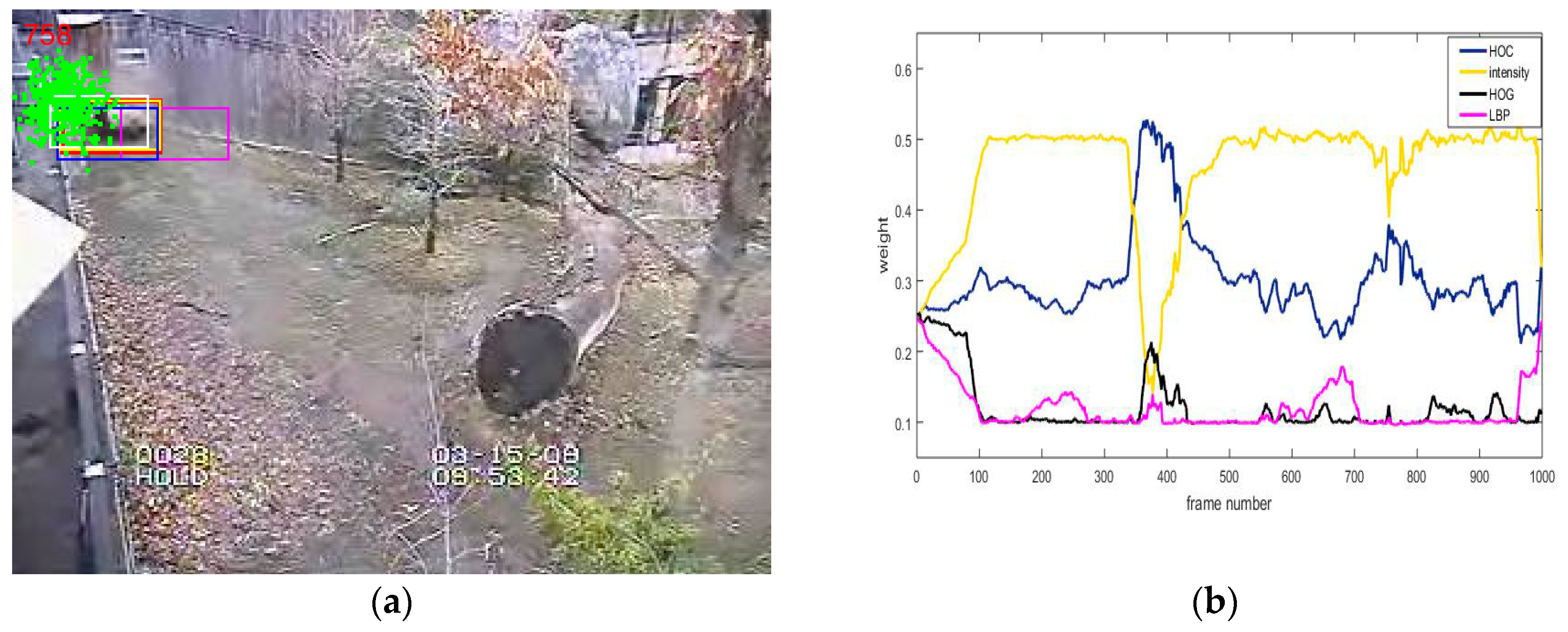
In complex scenes, it is difficult to accurately represent the target with a single feature, which may lead to tracking drift or even failure. On the basis of the multi-feature fusion approach that has been proposed in the MTMVT algorithm, we utilized four complementary features (histogram of color (HOC), intensity, HOG, and LBP) to represent the target, and to propose an adaptive multi-feature fusion strategy, as shown in Figure 3a.
In multi-feature tracking algorithms, the simple addition of the tracking result of each feature does not make full use of the advantages of the multiple features. Meanwhile, the robustness of each feature to the different scenes is different. When the robustness of a feature to a scene is high, the weight of the feature should be increased; otherwise, the weight of the feature should be reduced. As shown in Figure 3b, it can be seen that the weights of the four features change during the tracking of the Panda sequence. The weight of the feature is calculated by the following method.
In the first frame, set the weight of each feature to be the same, as follows:
where denotes the number of the frame. From the second frame, the new weight is updated by the similarity between the particle with the highest similarity, which is calculated according to the j-th feature and the particle with the highest similarity, which is calculated according to all of the features. The expression of this similarity between the particles is as follows:
where is a constant for controlling the shape of the Gaussian kernel, and is defined as follows:
where represents the state (affine parameter) of the jbest-th particle, which has the highest similarity and is calculated according to the j-th feature, and ; represents the state (affine parameter) of the i-th particle, which has the highest similarity to the target template and is calculated according to all of the features, and . Then, the expression of , which calculates the angle between two vectors is as follows:
The larger the angle, the greater the difference between the state of the particle with the highest similarity corresponding to the j-th feature, and the state of the particle calculated according to all of the features, or, the farther the two particles are apart from each other, or the greater the difference in their scale or post. Conversely, the smaller the angle, the closer the state of the particle with the highest similarity corresponding to the j-th feature to the state of the particle that is calculated according to all of the features, and the more reliable the j-th feature is been considered. The jbest-th particle corresponding to can be obtained by minimizing the sparse representation error corresponding to Equation (15), and the i-th particle corresponding to can be obtained by minimizing the sparse error corresponding to Equation (16).
where denotes the sparse representation error of the jbest-th particle determined by the j-th feature, denotes the sparse error of the i-th particle determined by all of the features, and is the sparse coefficient of the jbest-th particle corresponding to the j-th feature according to Equation (10). Finally, the feature weight is updated as follows:
In the proposed intelligent particle filter framework, in order to obtain a more reasonable target state in the first parts of the particles, we simultaneously considered the state of the particle with the highest similarity corresponding to each feature, and the state of the particle with the highest similarity corresponding to all of the features. Then, the expression of the state of the candidate target is as follows:
where is defined as the following:
where represents the number of features in the top of the sparse representation errors corresponding to the jbest-th particle, in addition to the j-th feature, in ascending order. The larger is, the more reliable the j-th feature is, and the more reliable the jbest-th particle is.
The second part of the particles are put according to the affine parameters that have been obtained by Equation (18), and the state of the final candidate target is determined by the following steps. Firstly, find out the top two features of the weights using Equation (17). Then, directly add the sparse errors corresponding to these two features. Finally, the particle with the smallest error is determined as the state of the target.
5. Experiment and Analysis
In order to verify the effectiveness of the proposed tracker, 10 typical trackers, including SCM [30], L1-APG [8], STC [31], CSK [32], MTT [33], CT [34], DFT [35], LOT [36], LRT [10], and MTMVT [15] were compared with our tracker, and 50 different challenging benchmark video sequences [37] were selected for testing. The experiments were carried out in MATLAB R2016b software installed on a 64-bit Windows OS, which ran on an Intel(R) Xeon(R) E3-1505M v5 CPU @2.80GHz, with 8G of memory.
5.1. Setting Parameters
The parameters that were involved in the experiments were set as follows: the template size was 12 × 15 for Lp-IPFT and the template size was 15 × 15 for AMFLp-IPFT, the affine transformation parameters of the particles put for the first time were 0.03, 0.0005, 0.0005, 0.03, 3.5, and 3.5, and the affine transformation parameters of the particles put for the second time were 0.005, 0.0005, 0.0005, 0.005, 0.8, and 0.8. In Equation (10), , , . In the intelligent particle filter algorithm, the total number of particles were n0 = 500, the number of the particles that were put for the first time were n1 = 450, the number of the particles that were put for the second time were n2 = 50. In Algorithm 1, the number of the trivial template was , the number of the positive template was , and the Lipchitz constant was . In the multi-feature fusion strategy, and . The proposed AMFLp-IPFT algorithm ran at 0.45 frames per second, and the Lp-IPFT algorithm ran at 25 frames per second.
5.2. Quantitative Analysis
The performance of our approach was quantitatively validate by two metrics, including distance precision (DP) and overlap success (OS) in a one-pass evaluation (OPE). The DP was defined as the percentage of frames where the distance precision (DP) and overlap success (OS)center location error (CLE) was within a threshold of 20 pixels. The OS was defined as the percentage of frames where the bounding box overlap surpassed a threshold of 0.5. The CLE was , where is the central location of the target tracked by the algorithm, and is the real center location of the target. The region area overlap ratio is defined as , where and are the tracked bounding box and the ground truth bounding box, respectively.
5.2.1. Overall Performance Analysis
We plotted the precision and success plots, including the area-under-the curve (ACU) score over all of the 50 sequences, as shown in Figure 4. It could be seen from Figure 4 that the proposed AMFLp-IPFT was superior to the other trackers. Table 2 illustrates that our algorithm performed favorably against the competitive trackers. The AMFLp-IPFT performed well against the Lp-IPFT (by 17.9% and 13.9%), MTMVT (by 21.0% and 28.0%), and L1-APG (by 53.7% and 40.4%), in terms of DP and OS, respectively. Compared with L1-APG, Lp-IPFT registered a performance improvement of 35.8% in terms of OS and 26.5% in terms of DP.
5.2.2. Attribute-Based Performance Analysis
In order to fully evaluate the effectiveness of the proposed algorithms, we further evaluated the performance of the algorithm using 11 attributes on the OTB-50 video dataset. All of the ACU results for each tracker were given in Table 3 and Table 4. The best result was highlighted in the red and the second was highlighted in blue.
We noted that the proposed AMFLp-IPFT performed well in handling challenging factors, including fast motion (precision plots: 62.9% and success plots: 49.7%), illumination variation (precision plots: 71.4% and success plots: 52.8%), and out-of-plane rotation (precision plots: 70.6% and success plots: 52.3%). The Lp-IPFT performed well in dealing with fast motion (precision plots: 54.2% and success plots: 44.1%) and low resolution (precision plots: 66.3% and success plots: 47.5%) challenging factors.
5.3. Qualitative Analysis
In view of the different characteristics of these video sequences mentioned above, we discussed four group experiments on eight video sequences with the 12 trackers that were described above.
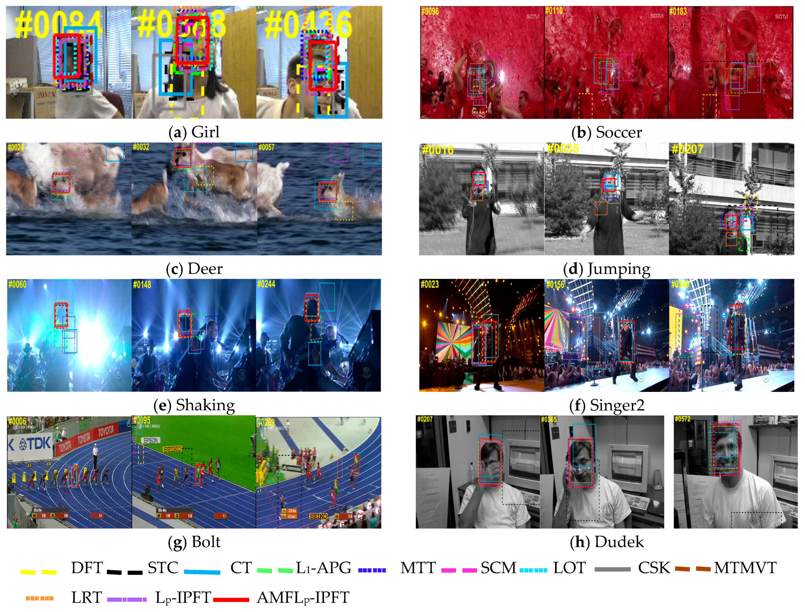
Experiment 1: Robustness analysis of partial occlusion
There were partial occlusion challenges in the short time in the Figure 5a Girl and Figure 5b Soccer video sequences. In the Girl sequence, there was an occlusion of a man’s head, as in frame 436. In the Soccer sequence, there were occlusions of red papers, as in frame 110 and 183, and an occlusion of the trophy at frame 96. For these videos, the Lp-IPFT, L1-APG, and SCM algorithms all only used the intensity feature and utilized trivial templates to judge occlusion, but in the complex scenes, the trivial templates were prone to misjudgment and the templates could not update in time. The proposed AMFLp-IPFT algorithm had a better tracking performance.
Experiment 2: Robustness analysis of fast motion
There were fast motion challenges in the Figure 5c Deer and Figure 5d Jumping video sequences. In the Deer sequence, the target moved significantly around the 32nd frame, and there was motion blur around the 24th frame and the 57th frame. In the Jumping sequence, there also existed fast motion and motion blur, as in frame 16, 35, and 207. For the fast motion challenge, the proposed intelligent particle filter enabled more particles to cover the target, so the Lp-IPFT and AMFLp-IPFT algorithms could solve the fast motion problem well, and further improved the robustness and accuracy of the tracking.
Experiment 3: Robustness analysis of illumination variation
There were illumination variation challenges in the Figure 5e Shaking and Figure 5f Singer2 video sequences. In the Shaking sequence, the targets were all affected by the background lighting, such as the 60th frame in the Shaking sequence and the 156th and 349th in the Singer2 sequence. Since the color feature was sensitive to illumination, it was not able to adapt to complex scenes with illumination variation. However, the LBP feature could make up for this deficiency, and it could overcome the influence of illumination variation. In addition, the HOG feature was also robust to the illumination variation. Therefore, the proposed AMFLp-IPFT algorithm had good tracking results to these sequences.
Experiment 4: robustness analysis of deformation
There were deformation challenges in the Figure 5g Bolt and Figure 5h Dudek video sequences. The targets’ limbs changed during the tracking, as in frame 6, 95, and 269 of the Bolt sequence. In addition, there was some change in facial expression, such as in the 572th frame of the Dudek sequence. Since the HOG feature maintained a good invariance of the target’s deformation in geometry and illumination, some movements of the subtle body could be ignored by the HOG feature without affecting the detection result. While the target had a large deformation, other features, such as color histograms, guaranteed that the final tracking result did not greatly deviate from the actual target.
6. Conclusions
In order to enhance the tracking performance, we improved the L1-APG tracker [8]. Firstly, we divided the particles into two parts and put them separately. In this way, the intelligent particles could cooperate with each other to achieve accurate tracking. Then, to get a sparser solution, a novel minimization model for the Lp tracker was proposed. Finally, an adaptive multi-feature fusion strategy was proposed to solve the problem that single feature could not deal with complex scenes ideally. The experimental results on a benchmark with 50 challenging sequences validated that the proposed AMFLp-IPFT algorithm had a better accuracy and robustness than several state-of-the-art trackers, for challenges such as fast motion, occlusion, illumination, and deformation. However, since the AMFLp-IPFT algorithm utilized four features to represent the target at the same time, the real-time performance could not be satisfied. Therefore, how to improve the tracking efficiency was the work that needed to be researched in the next step.
Author Contributions
Conceptualization, D.H. and Y.L.; methodology, Y.L. and D.H.; software, Y.L.; validation, Y.L., and W.H.; formal analysis, Y.L.; investigation, Y.L.; resources, Y.L.; data curation, W.H.; writing (original draft preparation), Y.L.; writing (review and editing), D.H.; visualization, Y.L.; supervision, D.H.; project administration, D.H.; and funding acquisition, D.H.
Funding
This research was funded by the Nature Science Foundation of China (Grant No. 61672335, No. 61602191), by the Foundation of Fujian Education Department under Grand No. JAT170053.
Acknowledgments
This work is supported by the Nature Science Foundation of China (Grant No. 61672335, No. 61602191), by the Foundation of Fujian Education Department under Grand No. JAT170053. The authors would like to thank the reviewers for their valuable suggestions and comments.
Conflicts of Interest
The authors declare no conflict of interest.
References
- Yilmaz, A. Object tracking: A survey. ACM Comput. Surv. 2006, 38, 81–93. [Google Scholar] [CrossRef]
- Smeulders, A.W.; Chu, D.M.; Cucchiara, R.; Calderara, S.; Dehghan, A.; Shah, M. Visual Tracking: An Experimental Survey. IEEE Trans. Pattern Anal. Mach. Intell. 2014, 36, 1442–1468. [Google Scholar] [PubMed] [Green Version]
- Che, Z.; Hong, Z.; Tao, D. An Experimental Survey on Correlation Filter-based Tracking. In Proceedings of the IEEE Conference on Computer Vision and Pattern Recognition, San Diego, CA, USA, 20–25 June 2005; pp. 1–13. [Google Scholar]
- Li, H.; Shen, C.; Shi, Q. Real-time visual tracking using compressive sensing. In Proceedings of the IEEE Conference on Computer Vision and Pattern Recognition, Providence, RI, USA, 20–25 June 2011; pp. 1305–1312. [Google Scholar]
- Mei, X.; Ling, H.B. Robust visual tracking and vehicle classification via sparse representation. IEEE Trans. Pattern Anal. Mach. Intell. 2011, 33, 2259–2272. [Google Scholar] [PubMed]
- Mei, X.; Ling, H.B. Robust Visual Tracking Using L1 Minimization. In Proceedings of the IEEE International Conference on Computer Vision, Kyoto, Japan, 29 September–2 October 2009; pp. 1436–1443. [Google Scholar]
- Mei, X.; Ling, H.B.; Wu, Y.; Blasch, E.; Bai, L. Minimum error bounded efficient L1 tracker with occlusion detection. In Proceedings of the IEEE Conference on Computer Vision and Pattern Recognition, Providence, RI, USA, 20–25 June 2011; pp. 1257–1264. [Google Scholar]
- Bao, C.L.; Wu, Y.; Ling, H.B.; Ji, H. Real time robust L1 tracker using accelerated proximal gradient approach. In Proceedings of the IEEE Conference on Computer Vision and Pattern Recognition, Providence, RI, USA, 16–21 June 2012; pp. 1830–1837. [Google Scholar]
- Zhang, T.; Liu, S.; Ahuja, N.; Yang, M.H.; Ghanem, B. Robust visual tracking via consistent low-rank sparse learning. Int. J. Comput. Vis. 2014, 111, 171–190. [Google Scholar] [CrossRef]
- Zhang, T.; Ghanem, B.; Liu, S.; Ahuja, N. Low-rank sparse learning for robust visual tracking. In Proceedings of the European Conference on Computer Vision, Florence, Italy, 7–13 October 2012; pp. 470–484. [Google Scholar]
- Yang, Y.; Hu, W.; Xie, Y.; Zhang, W.; Zhang, T. Temporal Restricted Visual Tracking via Reverse-Low-Rank Sparse Learning. IEEE Trans. Cybern. 2017, 47, 485–498. [Google Scholar] [CrossRef] [PubMed]
- Chartrand, R. Fast algorithms for nonconvex compressive sensing: MRI reconstruction from very few data. In Proceedings of the IEEE International Symposium on Biomedical Imaging: From Nano to Macro, Boston, MA, USA, 28 June–1 July 2009; pp. 262–265. [Google Scholar]
- Zuo, W.; Meng, D.; Zhang, L.; Feng, X.; Zhang, D. A generalized iterated shrinkage algorithm for non-convex sparse coding. In Proceedings of the IEEE International Conference on Computer Vision, Sydney, NSW, Australia, 1–8 December 2013; pp. 217–224. [Google Scholar]
- Chartrand, R. Shrinkage mappings and their induced penalty functions. In Proceedings of the IEEE International Conference on Acoustics, Speech and Signal, Florence, Italy, 4–9 May 2014; pp. 1026–1029. [Google Scholar]
- Hong, Z.; Mei, X.; Prokhorov, D.; Tao, D. Tracking via Robust Multi-task Multi-view Joint Sparse Representation. In Proceedings of the IEEE International Conference on Computer Vision, Sydney, NSW, Australia, 1–8 December 2013; pp. 649–656. [Google Scholar]
- Kwon, J.; Lee, K.M. Visual tracking decomposition. In Proceedings of the IEEE Conference on Computer Vision and Pattern Recognition, San Francisco, CA, USA, 13–18 June 2010; pp. 1269–1276. [Google Scholar]
- Zhang, S.P.; Zhou, H.Y.; Jiang, F.; Li, X. Robust Visual Tracking Using Structurally Random Projection and Weighted Least Squares. IEEE Trans Circuits Syst. Video Technol. 2015, 25, 1749–1760. [Google Scholar] [CrossRef]
- Meshgi, K.; Maeda, S.I.; Oba, S.; Skibbe, H.; Li, Y.Z.; Ishii, S. An occlusion-aware particle filter tracker to handle complex and persistent occlusions. Comput. Vis. Image Underst. 2016, 150, 81–94. [Google Scholar] [CrossRef]
- Zhang, H.; Wang, L.; Yan, B.; Lei, L.; Cai, A.; Hu, G. Constrained Total Generalized p-Variation Minimization for Few-View X-Ray Computed Tomography Image Reconstruction. PLoS ONE 2016, 11, e0149899. [Google Scholar] [CrossRef] [PubMed]
- Xie, Y.; Gu, S.; Liu, Y.; Zuo, W.; Zhang, W.; Zhang, L. Weighted Schatten, p-Norm Minimization for Image Denoising and Background Subtraction. IEEE Trans. Image Process. 2016, 25, 4842–4857. [Google Scholar] [CrossRef]
- Wang, W.; Zhang, H.; Zhu, P.; Zhang, D.; Zuo, W. Non-convex Regularized Self-representation for Unsupervised Feature Selection. In Proceedings of the International Conference on Intelligent Science and Big Data Engineering, Suzhou, China, 14–16 June 2015; Volume 9243, pp. 55–65. [Google Scholar]
- Chartrand, R. Nonconvex Splitting for Regularized Low-Rank + Sparse Decomposition. IEEE Trans. Signal Process. 2012, 60, 5810–5819. [Google Scholar] [CrossRef]
- Dash, P.P.; Patra, D.; Mishra, S.K. Local Binary Pattern as a Texture Feature Descriptor in Object Tracking Algorithm. In Intelligent Computing, Networking, and Informatics; Springer: India, Pune, 2014; pp. 541–548. [Google Scholar]
- Yoon, J.H.; Kim, D.Y.; Yoon, K.J. Visual tracking via adaptive tracker selection with multiple features. In Proceedings of the 12th European Conference on Computer Vision, Florence, Italy, 7–13 October 2012; pp. 28–41. [Google Scholar]
- Morenonoguer, F.; Sanfeliu, A.; Samaras, D. Dependent Multiple Cue Integration for Robust Tracking. IEEE Trans. Pattern Anal. Mach. Intell. 2008, 30, 670–685. [Google Scholar] [CrossRef] [PubMed] [Green Version]
- Yin, M.; Zhang, J.; Sun, H.; Gu, W. Multi-cue-based CamShift guided particle filter tracking. Exp. Syst. Appl. 2011, 38, 6313–6318. [Google Scholar] [CrossRef]
- Zhao, S.; Wang, W.; Ma, S.; Zhang, Y.; Yu, M. A fast particle filter object tracking algorithm by dual features fusion. Proc. SPIE 2014, 9301, 1–8. [Google Scholar]
- Tian, P. A particle filter object tracking based on feature and location fusion. In Proceedings of the IEEE International Conference on Software Engineering and Service Science, Beijing, China, 23–25 September 2015; pp. 762–765. [Google Scholar]
- Tseng, P. On accelerated proximal gradient methods for convex-concave optimization. SIAM J. Opt. 2008. [Google Scholar]
- Zhong, W.; Lu, H.; Yang, M.H. Robust object tracking via sparsity-based collaborative model. In Proceedings of the IEEE Conference on Computer Vision and Pattern Recognition, Providence, RI, USA, 16–21 June 2012; pp. 1838–1845. [Google Scholar]
- Zhang, K.; Zhang, L.; Liu, Q.; Zhang, D.; Yang, M.H. Fast Visual Tracking via Dense Spatio-temporal Context Learning. In Proceedings of the 13th European Conference on Computer Vision, Zurich, Switzerland, 6–12 September 2014; Springer: Cham, Switzerland, 2014; Volume 8693, pp. 127–141. [Google Scholar]
- Caseiro, R.; Martins, P.; Batista, J. Exploiting the Circulant Structure of Tracking-by-Detection with Kernels. In Proceedings of the 12th European Conference on Computer Vision, Florence, Italy, 7–13 October 2012; pp. 702–715. [Google Scholar]
- Zhang, T.; Ghanem, B.; Liu, S.; Ahuja, N. Robust visual tracking via structured multi-task sparse learning. Int. J. Comput. Vis. 2013, 101, 367–383. [Google Scholar] [CrossRef]
- Zhang, K.; Zhang, L.; Yang, M.H. Real-time compressive tracking. In Proceedings of the 12th European Conference on Computer Vision, Florence, Italy, 7–13 October 2012; pp. 866–879. [Google Scholar]
- Laura, S.L.; Erik, L.M. Distribution fields for tracking. In Proceedings of the IEEE Conference on Computer Vision and Pattern Recognition, Providence, RI, USA, 16–21 June 2012; pp. 1910–1917. [Google Scholar]
- Avidan, S.; Levi, D.; BarHillel, A.; Oron, S. Locally Orderless Tracking. In Proceedings of the IEEE Conference on Computer Vision and Pattern Recognition, Providence, RI, USA, 16–21 June 2012; pp. 1940–1947. [Google Scholar]
- Wu, Y.; Lim, J.; Yang, M.H. Online Object Tracking: A Benchmark. In Proceedings of the IEEE Conference on Computer Vision and Pattern Recognition, Portland, OR, USA, 23–28 June 2013; pp. 2411–2418. [Google Scholar]
Figure 1.
The details of particles put in the third frame of the Deer sequence. All of the particles are divided into two parts and put separately, the red particles indicate the particles put for the first time, and the green particles indicate the particles put for the second time, and the location of the particle is assumed to correspond to the upper left corner of the tracked bounding box. Firstly, the first part particles (red particles) are put according to the target state of the second frame, and the locations of these particles are in accordance with the Gaussian distribution. Then, the similarity of each red particle to the template is calculated, and the second part particles (green particles) are put at the location of the red particle with the highest similarity, and the locations of the green particles are still in accordance with the Gaussian distribution. Finally, the similarity of each green particle is calculated, and the most similar particle (including red and green particles) is selected as the candidate target. When the particles are put in the fourth frame, the same method as the third frame is utilized. It can be seen that the most similar red particle has been close to the target, and then using the green particles to cover the target, which can make the number of the particles that are distributed around the target as many as possible.
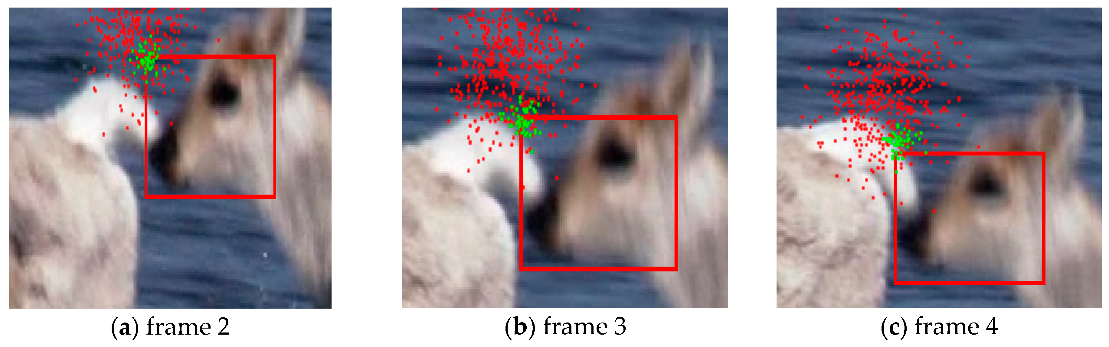
Figure 2.
Lp norm. (a) ; (b) ; and (c) . , .

Figure 3.
In (a), the red bounding box represents the final target state, the blue one represents the most similar particle to the target template for the histogram of color (HOC) feature, the yellow one represents the most similar particle to the target template for the intensity feature, the white one represents the most similar particle to the target template for the histogram of oriented gradient (HOG) feature, and the purple one represents the most similar particle to the target template for the LBP feature; (b) Is the variation curve of the weights of different features during the tracking of the Panda sequence (in this paper, we set the upper and lower limits of the weight, with a maximum of 0.5 and a minimum of 0.1).

Figure 4.
Comparisons of different trackers by using precision and success plots over all 50 sequences. The legend contains the ACU score for each tracker.
Figure 4.
Comparisons of different trackers by using precision and success plots over all 50 sequences. The legend contains the ACU score for each tracker.
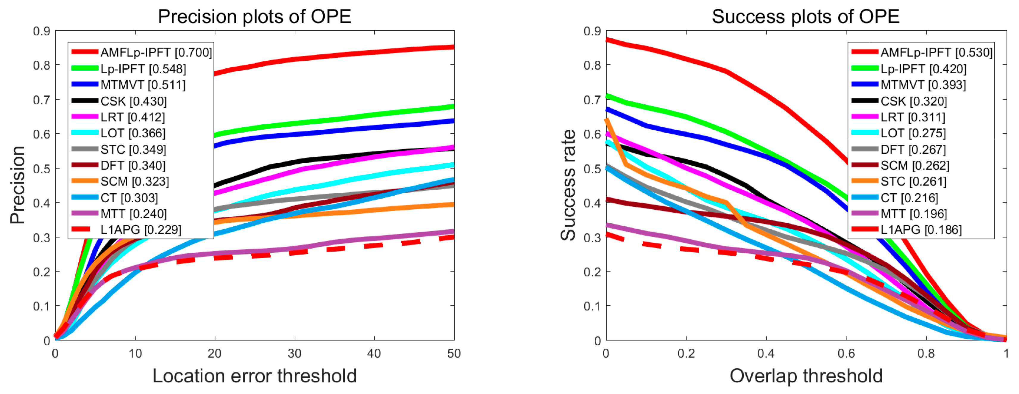
Figure 5.
Four groups of tracking results corresponding to different trackers.


Table 1.
The center location error (CLE) average of the L0.5-accelerated proximal gradient (APG) and L1-APG on 8 video sequences.
Table 1.
The center location error (CLE) average of the L0.5-accelerated proximal gradient (APG) and L1-APG on 8 video sequences.
| Tracker | Car4 | David2 | Dog | Dudek | Deer | Girl | Surfer | Trellis |
|---|---|---|---|---|---|---|---|---|
| L1-APG | 4.870 | 2.857 | 11.50 | 22.55 | 25.69 | 4.14 | 44.42 | 62.20 |
| L0.5-APG | 2.019 | 3.913 | 8.951 | 25.42 | 11.22 | 3.913 | 8.024 | 28.841 |
Note: The description of CLE is in the Section 5.
Table 2.
Quantitative comparison of 12 trackers on 50 sequences.
| SCM | L1-APG | STC | CSK | MTT | CT | DFT | LOT | MTMVT | LRT | Lp-IPFT | AMFLp-IPFT | |
|---|---|---|---|---|---|---|---|---|---|---|---|---|
| DP | 0.341 | 0.237 | 0.379 | 0.449 | 0.251 | 0.308 | 0.346 | 0.376 | 0.564 | 0.426 | 0.595 | 0.774 |
| OS | 0.319 | 0.220 | 0.251 | 0.348 | 0.238 | 0.214 | 0.284 | 0.297 | 0.471 | 0.344 | 0.485 | 0.624 |
Note: The maximum distance precision (DP) and overlap success (OS) values are highlighted in red type, and the second ones are highlighted in light blue type. MTMVT—multi-task multi-view tracking algorithm.
Table 3.
ACU results of each tracker on sequences with different challenge for OPE about precision.
| Challenge | SCM | L1-APG | STC | CSK | MTT | CT | DFT | LOT | MTMVT | LRT | Lp-IPFT | AMFLp-IPFT |
|---|---|---|---|---|---|---|---|---|---|---|---|---|
| BC | 0.310 | 0.223 | 0.331 | 0.419 | 0.226 | 0.245 | 0.357 | 0.325 | 0.512 | 0.416 | 0.420 | 0.695 |
| FM | 0.167 | 0.158 | 0.175 | 0.339 | 0.173 | 0.240 | 0.231 | 0.352 | 0.442 | 0.310 | 0.542 | 0.629 |
| MB | 0.166 | 0.134 | 0.210 | 0.382 | 0.131 | 0.230 | 0.224 | 0.328 | 0.438 | 0.321 | 0.572 | 0.651 |
| DEF | 0.246 | 0.170 | 0.313 | 0.373 | 0.172 | 0.247 | 0.338 | 0.353 | 0.474 | 0.315 | 0.427 | 0.680 |
| IV | 0.441 | 0.217 | 0.424 | 0.459 | 0.241 | 0.259 | 0.367 | 0.297 | 0.489 | 0.399 | 0.442 | 0.714 |
| IPR | 0.320 | 0.235 | 0.337 | 0.411 | 0.249 | 0.340 | 0.322 | 0.337 | 0.527 | 0.490 | 0.565 | 0.707 |
| LR | 0.128 | 0.177 | 0.362 | 0.369 | 0.183 | 0.364 | 0.278 | 0.233 | 0.421 | 0.488 | 0.663 | 0.659 |
| OCC | 0.390 | 0.270 | 0.353 | 0.424 | 0.272 | 0.379 | 0.372 | 0.403 | 0.441 | 0.446 | 0.505 | 0.686 |
| OPR | 0.384 | 0.237 | 0.356 | 0.388 | 0.248 | 0.357 | 0.363 | 0.392 | 0.490 | 0.447 | 0.482 | 0.706 |
| OV | 0.231 | 0.233 | 0.285 | 0.368 | 0.265 | 0.391 | 0.295 | 0.347 | 0.439 | 0.426 | 0.542 | 0.638 |
| SV | 0.321 | 0.204 | 0.336 | 0.388 | 0.205 | 0.317 | 0.313 | 0.333 | 0.461 | 0.403 | 0.561 | 0.665 |
Note: The best result was highlighted in the red and the second was highlighted in blue.
Table 4.
ACU results of each tracker on sequences with different challenge for OPE about success.
| Challenge | SCM | L1-APG | STC | CSK | MTT | CT | DFT | LOT | MTMVT | LRT | Lp-IPFT | AMFLp-IPFT |
|---|---|---|---|---|---|---|---|---|---|---|---|---|
| BC | 0.259 | 0.193 | 0.250 | 0.332 | 0.201 | 0.220 | 0.306 | 0.247 | 0.417 | 0.327 | 0.329 | 0.539 |
| FM | 0.143 | 0.133 | 0.150 | 0.272 | 0.148 | 0.186 | 0.196 | 0.283 | 0.360 | 0.248 | 0.441 | 0.497 |
| MB | 0.136 | 0.110 | 0.182 | 0.306 | 0.111 | 0.178 | 0.193 | 0.265 | 0.360 | 0.274 | 0.463 | 0.515 |
| DEF | 0.194 | 0.141 | 0.232 | 0.279 | 0.142 | 0.202 | 0.277 | 0.257 | 0.358 | 0.245 | 0.314 | 0.498 |
| IV | 0.364 | 0.179 | 0.305 | 0.339 | 0.202 | 0.200 | 0.300 | 0.235 | 0.385 | 0.306 | 0.347 | 0.528 |
| IPR | 0.260 | 0.189 | 0.247 | 0.318 | 0.203 | 0.253 | 0.258 | 0.257 | 0.409 | 0.347 | 0.413 | 0.546 |
| LR | 0.113 | 0.154 | 0.199 | 0.251 | 0.157 | 0.214 | 0.196 | 0.169 | 0.297 | 0.304 | 0.475 | 0.467 |
| OCC | 0.313 | 0.216 | 0.245 | 0.296 | 0.220 | 0.263 | 0.275 | 0.297 | 0.325 | 0.316 | 0.380 | 0.498 |
| OPR | 0.310 | 0.189 | 0.247 | 0.281 | 0.202 | 0.257 | 0.278 | 0.292 | 0.370 | 0.319 | 0.363 | 0.523 |
| OV | 0.205 | 0.207 | 0.197 | 0.294 | 0.232 | 0.296 | 0.233 | 0.281 | 0.339 | 0.312 | 0.419 | 0.474 |
| SV | 0.261 | 0.166 | 0.276 | 0.276 | 0.169 | 0.220 | 0.236 | 0.251 | 0.346 | 0.293 | 0.427 | 0.498 |
Note: The best result was highlighted in the red and the second was highlighted in blue.
© 2018 by the authors. Licensee MDPI, Basel, Switzerland. This article is an open access article distributed under the terms and conditions of the Creative Commons Attribution (CC BY) license (http://creativecommons.org/licenses/by/4.0/).
Share and Cite
MDPI and ACS Style
Lin, Y.; Huang, D.; Huang, W. Target Tracking Algorithm Based on an Adaptive Feature and Particle Filter. Information 2018, 9, 140. https://doi.org/10.3390/info9060140
AMA Style
Lin Y, Huang D, Huang W. Target Tracking Algorithm Based on an Adaptive Feature and Particle Filter. Information. 2018; 9(6):140. https://doi.org/10.3390/info9060140
Chicago/Turabian StyleLin, Yanming, Detian Huang, and Weiqin Huang. 2018. "Target Tracking Algorithm Based on an Adaptive Feature and Particle Filter" Information 9, no. 6: 140. https://doi.org/10.3390/info9060140
Note that from the first issue of 2016, this journal uses article numbers instead of page numbers. See further details here.