How Uncertain Information on Service Capacity Influences the Intermodal Routing Decision: A Fuzzy Programming Perspective


School of Management Science and Engineering, Shandong University of Finance and Economics, No. 7366, Second Ring East Road, Jinan 250014, China
*
Authors to whom correspondence should be addressed.
Information 2018, 9(1), 24; https://doi.org/10.3390/info9010024
Submission received: 18 December 2017
/
Revised: 19 January 2018
/
Accepted: 23 January 2018
/
Published: 24 January 2018
(This article belongs to the Section Information Processes)
Abstract
:Capacity uncertainty is a common issue in the transportation planning field. However, few studies discuss the intermodal routing problem with service capacity uncertainty. Based on our previous study on the intermodal routing under deterministic capacity consideration, we systematically explore how service capacity uncertainty influences the intermodal routing decision. First of all, we adopt trapezoidal fuzzy numbers to describe the uncertain information of the service capacity, and further transform the deterministic capacity constraint into a fuzzy chance constraint based on fuzzy credibility measure. We then integrate such fuzzy chance constraint into the mixed-integer linear programming (MILP) model proposed in our previous study to develop a fuzzy chance-constrained programming model. To enable the improved model to be effectively programmed in the standard mathematical programming software and solved by exact solution algorithms, a crisp equivalent linear reformulation of the fuzzy chance constraint is generated. Finally, we modify the empirical case presented in our previous study by replacing the deterministic service capacities with trapezoidal fuzzy ones. Using the modified empirical case, we utilize sensitivity analysis and fuzzy simulation to analyze the influence of service capacity uncertainty on the intermodal routing decision, and summarize some interesting insights that are helpful for decision makers.
1. Introduction
Intermodal transportation utilizes various transportation modes (e.g., railway, road, and waterway) to realize the transportation of containers. It has been widely acknowledged to be a better means of transportation compared with the unimodal transportation in many aspects (e.g., transportation economy and sustainability) [1,2], especially in the long-haul transportation setting. The intermodal routing decision aims at selecting the best routes to move containers from their origins to destinations through an intermodal service network to fulfill customers’ transportation demands. With the rapid development and promotion of intermodal transportation in international trade, the intermodal routing problem is now at the forefront of transportation planning [3].
During the intermodal routing decision process, one of the challenges that decision makers need to deal with is how to consider the restriction of the service capacity on the intermodal route selection. In the existing literature, some studies do not consider the capacity constraint and formulated uncapacitated intermodal routing models to optimize their respective specific problems, e.g., Ziliaskopoulos and Wardell (2000) [4], Lam and Srikanthan (2002) [5], Boussedjra et al. (2004) [6], Xiong and Wang (2014) [7] and Sun and Chen (2013) [8], etc. However, the uncapacitated scenario is impossible to be realized in transportation practice due to the following aspects.
- (1)
- From the viewpoint of network topology, it is difficult (but not impossible) for transportation providers to assign adequate trucks and drivers to conduct all the road services on the arcs in the entire intermodal service network. Therefore, the road service capacity is limited.
- (2)
- The capacity of a railway freight train is restricted by the limited power of the locomotive and the limited effective length of the railway tracks at the railway freight stations. Moreover, similar to road services, there are not infinite railway services on the network arcs. The railway service capacity is hence also limited.
Consequently, the intermodal routing decision based on the uncapacitated modeling is unreliable, because the actual existing capacities of the transportation services on the planned routes have considerable possibility of being violated, which will consequently result in failure. Therefore, the intermodal service network is capacitated. Thus the essence of the intermodal routing decision is the effective utilization of the limited resources of transportation services [3]. The service capacity is an important issue that should not be neglected during the routing decision.
The majority of the current studies concentrated on the capacitated intermodal routing problem, e.g., Chang (2008) [9], Sun et al. (2008) [10], Kim et al. (2008) [11], Ayar and Yaman (2012) [12], Moccia et al. (2011) [13], Lei et al. (2014) [14], Sun and Lang (2015a, 2015b) [15,16] and Sun et al. (2016) [17], etc. In the capacitated intermodal routing literature, deterministic numbers are used to express the service capacities. A capacity constraint is built to ensure that the total containers loaded on a certain service should not exceed its payload (e.g., the capacity of service 1 on arc 2 is 50 TEUs where TEU is the unit of ISO standard containers, which means that the total containers from different transportation orders assigned to service 1 on arc 2 should not exceed 50 TEUs). Compared with uncapacitated intermodal routing, the consideration of service capacity better matches the transportation practice and can greatly improve the feasibility of the intermodal routing decision.
It is widely known that the intermodal routing decision should be made before the actual transportation starts [18]. During such a forward-looking decision process, decision makers cannot get exact information on all the transportation service capacities. First of all, the transportation services in the intermodal service network should also implement many other transportation tasks that fall out of the decision targets. Such tasks will occupy part of the capacities of the transportation services. However, predicting these tasks accurately is a heavy burden that is time-consuming and requires a lot of manpower. Consequently, it is infeasible to predict such transportation tasks and then deduct their occupied capacities from the total capacities. Secondly, there are many influencing factors that will also reduce the capacity utilization, e.g., vehicle faults, traffic accidents and bad weather. Therefore, it is difficult for decision makers to find a deterministic number to represent the capacity of a transportation service.
If decision makers insist on using deterministic numbers to represent the capacities of transportation services, two consequences will occur in the actual transportation if the containers are moved according to the intermodal routing decision with capacity certainty. The intermodal routing decision will be meaningless in this case.
- (1)
- Optimistic estimation: the deterministic capacities evaluated by decision makers are larger than the actual available capacities of the services, which are known only when the transportation starts. In this case, the planned intermodal routes may be infeasible because it is possible that some transportation services cannot carry the number of containers assigned to them according to the routing decision. Taking Figure 1 as an example, the estimated capacity values of the services on the road-railway-road intermodal route are 35 TEUs, 45 TEUs, and 30 TEUs (black). Based on these values, the route can move the containers with 30 TEUs from node 1 to node 4. However, since the estimation is optimistic, the actual values are smaller than the estimated ones. When the actual values are 25 TEUs, 30 TEUs and 20 TEUs (red), the route is infeasible because the road services on arc (1, 2) and arc (3, 4) cannot carry that number of containers. Thus, such route planning in the transportation practice failed. Consequently, under optimistic estimation, the planned route may be infeasible in practice.
- (2)
- Pessimistic estimation: the deterministic capacities evaluated by the decision makers are smaller than the available capacities of the services. In this case, the planned intermodal routes will be certainly feasible but may be not the best ones. Taking Figure 2 as an example, under pessimistic estimation, the best planned intermodal route is “(1) road service—(2) railway service—(3) road service—(4)”. The cost of the route is 2200 RMB. Since the estimation is pessimistic, the actual values are larger than the estimated ones. In this case, a railway service from node 2 to node 4 can be used to move the containers in practice. Thus, the actual best intermodal route would be “(1) road service—(2) railway service—(4)”. The cost of this route is 1800 RMB, which saves 400 RMB compared to the planned best route. Consequently, under a pessimistic estimation, the planned best route is feasible in practice but may not be the actual best scheme.
During the decision-making process, the situation will be more complicated due to the mixture of optimistic and pessimistic estimations of the service capacities. To avoid the consequences above, it is essential to fully consider the service capacity uncertainty in the intermodal routing decision to improve its reliability in supporting practical decision-making. However, according to the best of our knowledge, there are rare intermodal routing decision studies that systematically explore the influences of service capacity uncertainty on the intermodal routing decision, neither from a stochastic programming perspective nor a fuzzy programming perspective. Faced with such a research gap and in order to bridge it, this study mainly focuses on the following aspects:
- (1)
- How do we model the service capacity uncertainty in a way that is easily realized in transportation practice?
- (2)
- How do we analyze and summarize the influences of service capacity uncertainty on the intermodal routing decision?
In our previous study [15], we presented a mixed-integer nonlinear programming (MINLP) model and developed a linearization-based exact solution strategy to solve the multicommodity intermodal routing problem with schedule-based railway services and time-flexible road services. This study was oriented on a consideration of deterministic service capacity, but still provided a solid foundation for us to discuss the issues of service capacity uncertainty. All the explorations regarding this study are on the basis of the transportation scenario, modeling framework, and solution strategy from our previous study.
The remainder of this study is organized as follows. In Section 2, we formulate the service capacity uncertainty from the viewpoint of fuzziness and use trapezoidal fuzzy numbers to represent the uncertain service capacities. In Section 3, we model the fuzzy chance constraint of the service capacity based on the credibility measure and generate crisp equivalent linear reformulations of the fuzzy chance constraint. Then we can use the proposed reformulations to replace the deterministic capacity constraint in the MILP model constructed in our previous study [15] to create a linear programming model that focuses on the intermodal routing problem with service capacity uncertainty. In Section 4, we present a case study to show how service capacity uncertainty influences the intermodal routing decision with the help of sensitivity analysis and fuzzy simulation. Finally, the conclusions of this study are drawn in Section 5.
2. Modeling the Service Capacity Uncertainty
2.1. Capacity Uncertainty: Stochasticity vs. Fuzziness
Generally, there are two approaches to address the various uncertain issues (e.g., demand uncertainty [18,19,20] and travel time/length uncertainty [21,22,23]) in the transportation planning field, stochastic programming and fuzzy programming.
When using stochastic programming to formulate the uncertain service capacity constraint, first of all, we require a tremendous amount of reliable historical data to fit the probability distribution of the uncertain capacities of the transportation services in the intermodal service network [18,23]. Collecting and processing large-scale data during the decision-making process is cumbersome and costly. As indicated by Zarandi et al. (2008) [23], in most cases, there are not enough data to accomplish such a probability distribution. Moreover, limited data show that the variation of the service capacities, especially the railway service capacities, within a period does not observe regular tendencies. Thus, we cannot simply assume that the uncertainty of the service capacity follows a classic distribution form, e.g., normal distribution or Poisson distribution.
However, decision makers can easily use fuzzy logic knowledge to estimate the service capacity uncertainty based on their or other experts’ knowledge, experience, and judgment. As a result, it is worthwhile to try fuzzy estimation of the service capacity uncertainty when stochastic service capacity is unattainable. So, in this study, we model fuzzy service capacity instead of stochastic service capacity.
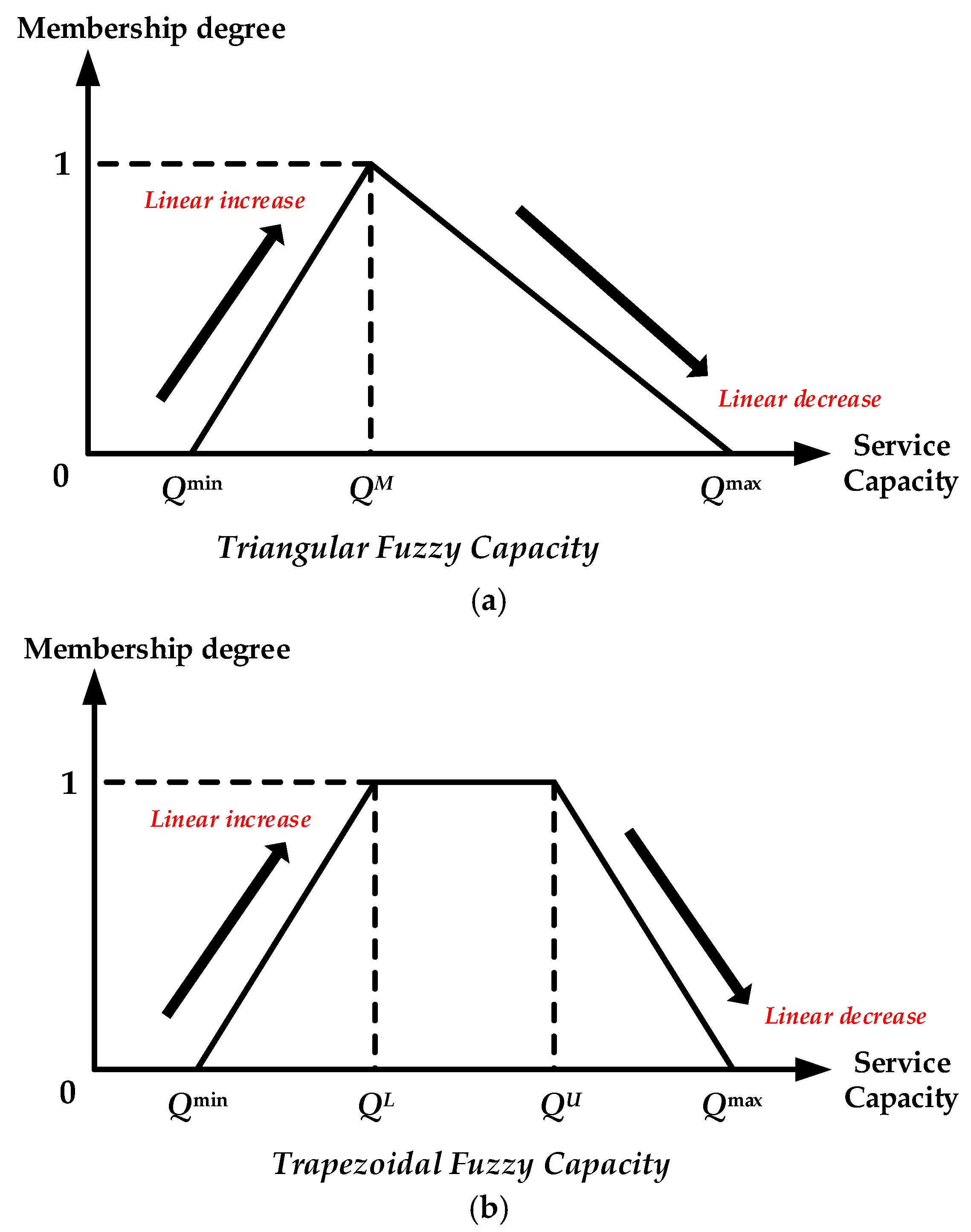
2.2. Fuzzy Service Capacity: Trapezoidal Fuzzy Numbers vs. Triangular Fuzzy Numbers
Trapezoidal or triangular fuzzy numbers can be used to represent the fuzzy service capacity (see Figure 3). As for a transportation service with fuzzy capacity , when represented by a trapezoidal fuzzy number, where and are the minimum and maximum of the all the possible capacity values, respectively, and and are the lower bound and upper bound of all the most likely capacity values. when formulated by a triangular fuzzy number, where is the most likely capacity value.
Compared with the triangular method, trapezoidal fuzzy capacity is preferable when considering the following advantages:
- (1)
- Using trapezoidal fuzzy capacity is more flexible for decision-making, allowing the existence of more than one most likely service capacity, which meets the practice that different decision makers and experts usually hold different opinions on the most likely values.
- (2)
- The trapezoidal fuzzy capacity can be easily approximated to a triangular one by significantly reducing the range of .
Above all, in this study, we formulate a trapezoidal fuzzy service capacity by Equation (1) to express the capacity uncertainty of the transportation services:
3. Fuzzy Chance Constraint of the Service Capacity
3.1. Deterministic Capacity Constraint
In intermodal routing modeling without capacity uncertainty, the deterministic capacity constraint is formulated as in Equation (3) [15]:
where k is the transportation order index, K is the transportation order set, (i,j) is the directed arc from node i to node j, A is the arc set in a given intermodal service network, s is the transportation service index, is the transportation service set on arc , is the containers of transportation order (unit: TEU), is the deterministic capacity of service on arc (unit: TEU), and is a 0–1 variable: if the containers of transportation order are planned to be moved on arc by service , = 1, otherwise 0. Equation (3) is a hard constraint and ensures that the following event must hold.
“As for a certain transportation service operated on the arc in the intermodal service network, the total number of the containers of all the transportation orders assigned to it by decision makers should not exceed its capacity.”
With the help of Equation (3), decision makers can design intermodal route schemes that can greatly reduce the possibility of violating the capacities. However, as claimed in Section 1, two negative consequences may still lower the feasibility in practice.
3.2. Fuzzy Chance Constraint
Using trapezoidal fuzzy numbers to represent the uncertain service capacity, the event represented by a deterministic capacity constraint is transformed into a fuzzy event. Furthermore, we can transform the deterministic capacity constraint Equation (3) into a fuzzy chance constraint based on one of the three fuzzy measures, possibility, necessity, and credibility measures. For detailed descriptions of the three fuzzy measures, refer to Zheng and Liu’s work (2008) on the fuzzy vehicle routing model [25].
According to Zheng and Liu (2008) [25] and Zarandi et al. (2008) [23], possibility and necessity measures lack the self-duality property, while the credibility measure is a self-dual measure. A fuzzy event may fail even if its possibility equals 1, and hold even if its necessity equals 0. However, the credibility measure can avoid such consequences, i.e., the fuzzy event must fail (hold) if its credibility equals 0 (1). So we construct the fuzzy chance constraint based on the credibility measure.
Based on the credibility measure [25,26], the fuzzy chance constraint of the service capacity is proposed as Equation (4):
In Equation (4), is the fuzzy capacity of transportation service on arc . The representations of the four parameters in are identical to these of , , and , respectively.
represents the credibility of the fuzzy incident in . The fuzzy chance constraint ensures that the creditability of the fuzzy incident in should not be smaller than confidence .
() is the confidence set by the decision makers during the decision-making process. It reflects the decision makers’ preference regarding the capacity uncertainty.
The values of significantly influence the intermodal routing results, which can be verified by using a sensitivity analysis in the case study section. Hence, determining the best value of for a certain case is of great significance, which will also be discussed by using fuzzy simulation in the same section.
In our previous study [15], we proposed a MINLP model to formulate the intermodal routing problem with schedule-based railway services and time-flexible road services. We then designed a linearization technique to generate an equivalent MILP model that can be solved by any exact solution algorithm implemented by any standard mathematical programming software. By replacing the deterministic capacity constraint in the MILP model with Equation (4), we can gain a fuzzy chance-constrained programming model to deal with the intermodal routing problem with service capacity uncertainty.
3.3. Crisp Equivalent Linear Reformulations of the Fuzzy Chance Constraint
Equation (4) cannot be directly programmed as a linear function in standard mathematical programming software. Thus the fuzzy chance-constrained programing model cannot be a straightforward input into the standard mathematical programming software and be solved by the exact solution algorithms. Therefore, we should first gain the crisp equivalent linear reformulation(s) of the fuzzy chance constraint Equation (4).
There are a deterministic and a trapezoidal fuzzy number where . According to Zarandi et al. (2008) [23], there exists following Equation (5) regarding :
By replacing a with and with , we can remove from the equation and gain the crisp equivalency (Equation (6)) to the fuzzy chance constraint (Equation (4)):
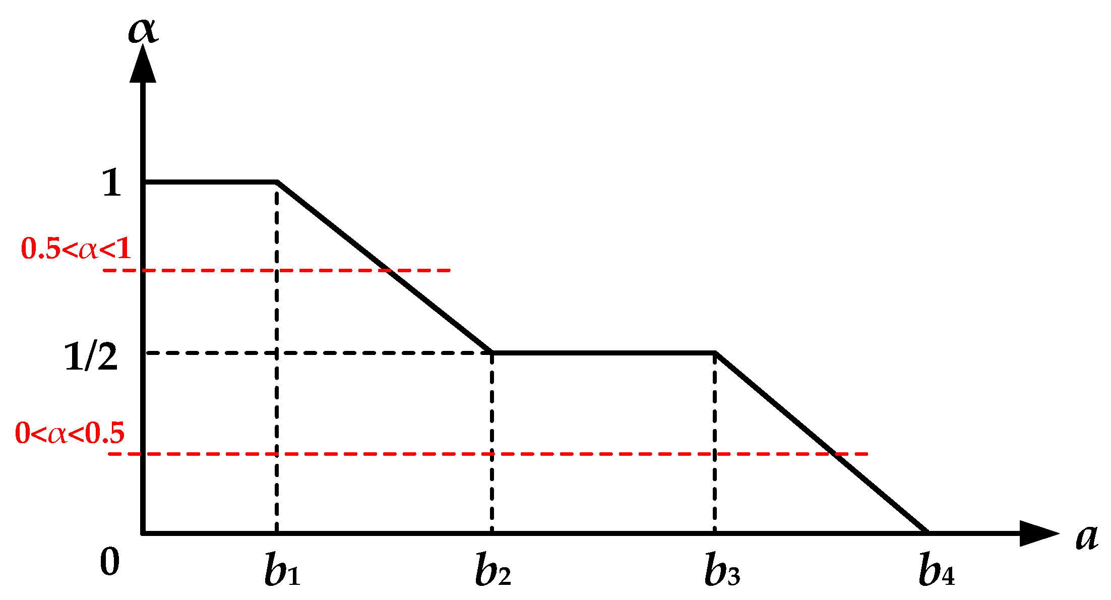
However, the crisp equivalency (Equation (6)) is still a nonlinear function. Then, according to the piecewise linear relationship between and in the credibility measure shown in Figure 4, we conduct the following modifications (Equations (7) and (8)) to gain crisp equivalent linear reformulations:
By replacing the fuzzy chance constraint (Equation (3)) with its crisp equivalent linear reformulations (Equations (7) and (8)), we can gain the crisp equivalent MILP model for the intermodal routing problem with fuzzy service capacity. The crisp equivalent MILP model can be effectively programmed in the mathematical programming software (e.g., LINGO) and solved by any exact solution algorithms (e.g., Branch-and-Bound Algorithm) to generate the global optimal solution to the problem.
4. Case Study
In this study, we modify the case study presented in our previous study [15] by replacing the deterministic capacities of the transportation services with trapezoidal fuzzy ones. Then the modified case can be used to explore how service capacity uncertainty influences the intermodal routing decision. For a detailed description of the empirical case, readers are referred to [15]. The trapezoidal fuzzy capacities of the transportation services in the intermodal service network are in Appendix A.
4.1. Simulation Environment
In this study, we use mathematical programming software LINGO version 12 (LINDO Systems Inc., Chicago, IL, USA) [27] to implement the Branch-and-Bound Algorithm to solve the intermodal routing problem with service capacity uncertainty that is formulated by the crisp equivalent MILP model. All the simulations in this study were run on a ThinkPad Laptop with Intel Core i5-5200U 2.20 GHz CPU 8 GB RAM. The scale of the case is shown in Table 1.
4.2. Illcesults
First of all, we set the confidence: = 0.9. The corresponding optimization results of the intermodal routing problem with service capacity uncertainty are indicated in Table 2. The best solution in Table 2 refers to the minimal generalized costs for routing the multiple commodity flows. The generalized costs include the transportation costs en route, the loading/unloading operation costs, the inventory costs, the additional pick-up and delivery costs, and the carbon dioxide emission costs.
4.3. Sensitivity Analysis to Indicate the Influence of the Confidence on the Routing Decision
Confidence in Equations (7) and (8) is determined by the decision makers during the intermodal routing decision process. The values of have a great effect on the optimization results generated by the optimization model, which can be investigated by using sensitivity analysis. In this analysis, the value of confidence varies from 0.1 to 1.0 with a step size of 0.1, and we can get the corresponding optimization results (best solution, i.e., the minimal generalized costs for transporting the multiple commodity flows) with respect to the variation, which is shown in Figure 5. From Figure 5, we can draw some interesting decisions, listed as follows.
- (1)
- The value of confidence influences the intermodal routing decision. Therefore, where to set the value is an important issue for decision makers.
- (2)
- In general, a stepwise increase of the minimal generalized costs for the intermodal routing decision emerges when the value of confidence increases linearly. Specifically in this case, the sensitivity of the intermodal routing with respect to confidence is especially significant when varies from 0.4 to 0.5 and from 0.8 to 0.9.
- (3)
- The transportation economy (reflected by the minimal generalized costs for the intermodal routing decision) and transportation reliability (reflected by the credibility of the intermodal routing decision) cannot reach an optimum simultaneously. The transportation economy will be reduced if the decision makers prefer higher reliability of the intermodal routing decision, and vice versa.
As a result, it is a challenging but meaningful task for decision makers to determine an objective value of confidence to make a tradeoff between the transportation economy and its reliability. Improving the transportation economy and meanwhile achieving reliable transportation is the objective of the intermodal routing decision with service capacity uncertainty.
4.4. Fuzzy Simulation to Determine the Best Confidence Value
We need to know the actual transportation to conduct the following procedures, so that the best confidence can be determined to realize the objective of the intermodal routing decision with service capacity uncertainty.
As claimed in Section 1, it is impossible for decision makers to master the capacity of actual transportation. We can, however, simulate the actual transportation scenario by using a fuzzy simulation. In the simulation, deterministic service capacities are randomly generated based on their fuzzy membership degree, shown as in Equation (2). The randomly generated capacities can be treated as the actual deterministic capacities of the transportation services in the intermodal service network. By using such capacities, we can realize Step 1 in Table 3. By inputting such capacities into the deterministic capacity constraint as in Equation (3), we can generate the actual best routes by using the MILP model from our previous study [15] and realize Step 2 in Table 3. The process of the fuzzy simulation is illustrated by Figure 6. In this study, we run the simulation 50 times in order to better match the transportation practice, and then use our knowledge of statistics to summarize some insights and determine the best value of confidence .
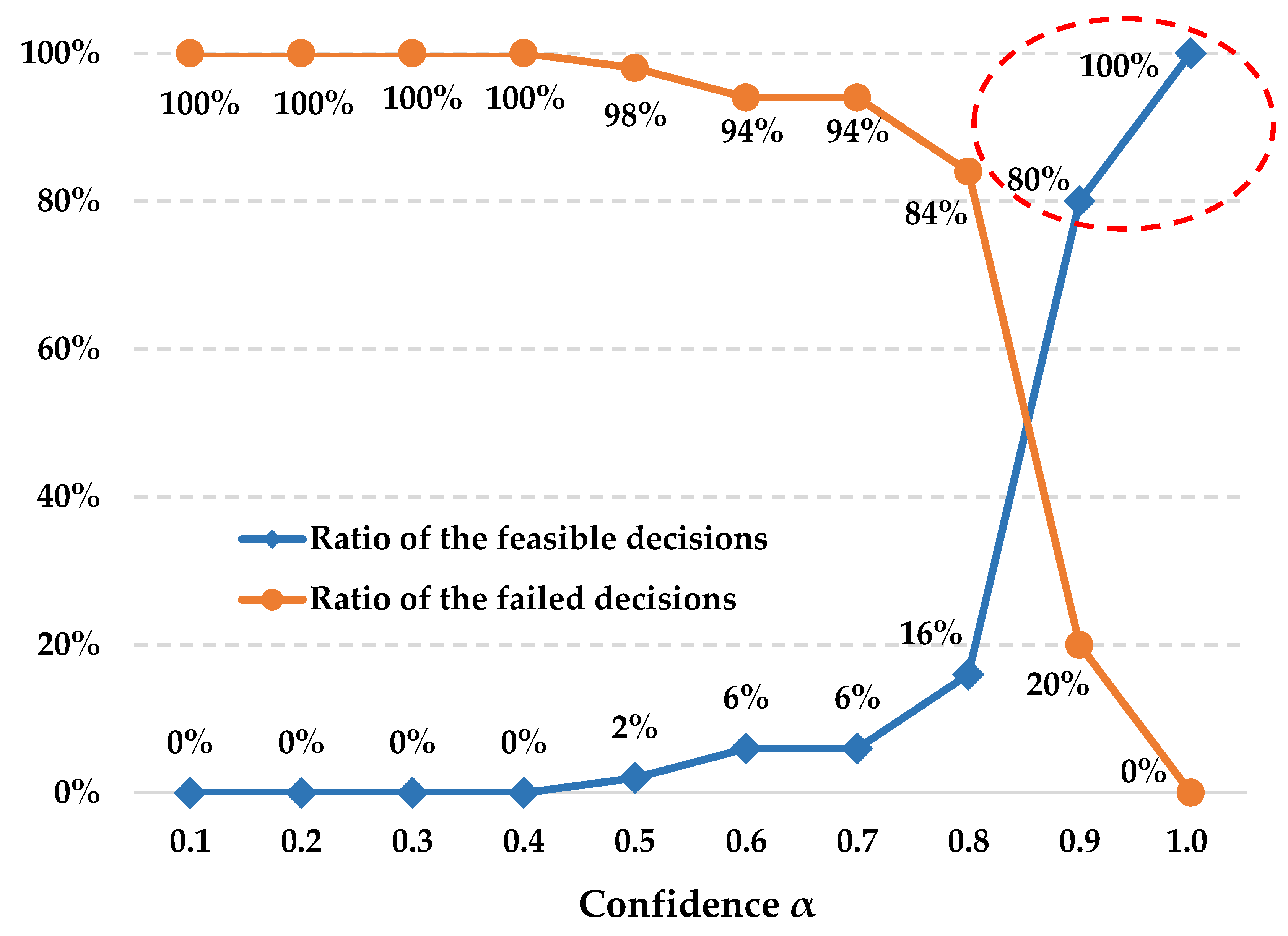
After getting the 50 sets of the actual service capacities, first of all, we check whether the planned best routes under different confidence values violate the capacity constraints corresponding to each service capacity set (i.e., implement Step 1 in Table 3 50 times for each confidence value). Then we can count the number of failed and feasible decisions given by the intermodal routing corresponding to each confidence value in the 50 simulations. The results are presented in Figure 7.
- (1)
- Overall, the ratio of the feasible decisions to the 50 simulations improves as confidence increases, i.e., the reliability of the intermodal routing decision gets enhanced by giving confidence a larger value.
- (2)
- The ratio of the feasible decisions improves slightly with the increase of confidence when it varies from 0.1 to 0.7, while it improves significantly when confidence exceeds 0.7.
- (3)
- The ratio of the feasible decisions greatly improves from 16% to 80% (by 400%) with a slight increase of the minimal generalized costs from 5,261,339 RMB to 5,339,867 RMB (by 1.5%) when confidence is set to 0.9 instead of 0.8. Thus, to maintain an acceptable transportation reliability, 0.9 and 1.0 are recommended as the values of confidence .
- (4)
- The ratio of the feasible decisions greatly improves from 16% to 100% (by 525%) with a slight increase of the minimal generalized costs from 5,261,339 RMB to 5,344,147 RMB (by 1.6%) when confidence is set to 1.0 instead of 0.8. Thus, to maintain an acceptable transportation reliability, 0.9 and 1.0 are recommended as the values of confidence .
In particular, the ratio of the feasible decisions improves from 80% to 100% (by 25%) with a relatively slight increase of the minimal generalized costs from 5,339,867 RMB to 5,344,147 RMB (by 0.08%) when confidence is set to 1.0 instead of 0.9.
In previous studies, decision makers use the most likely capacity to make intermodal routing decisions. So, in order to demonstrate the effectiveness of the approach proposed in this paper, we use the lower bound, upper bound, and the median value of the most likely capacity range to simulate the intermodal routing decision under deterministic capacity. The best solutions to the intermodal routing decisions under three deterministic capacity scenarios and corresponding ratios of feasible decisions in the 50 fuzzy simulations are given in Table 4. As shown in Table 4, under deterministic capacity scenarios, the ratios of the feasible decisions are 0%, which means that, as for this case, the feasibility of the intermodal routing decision will be dramatically improved by using the fuzzy programming approach proposed in this paper instead of the deterministic programming one used in previous studies. The effectiveness of the proposed approach is hence demonstrated.
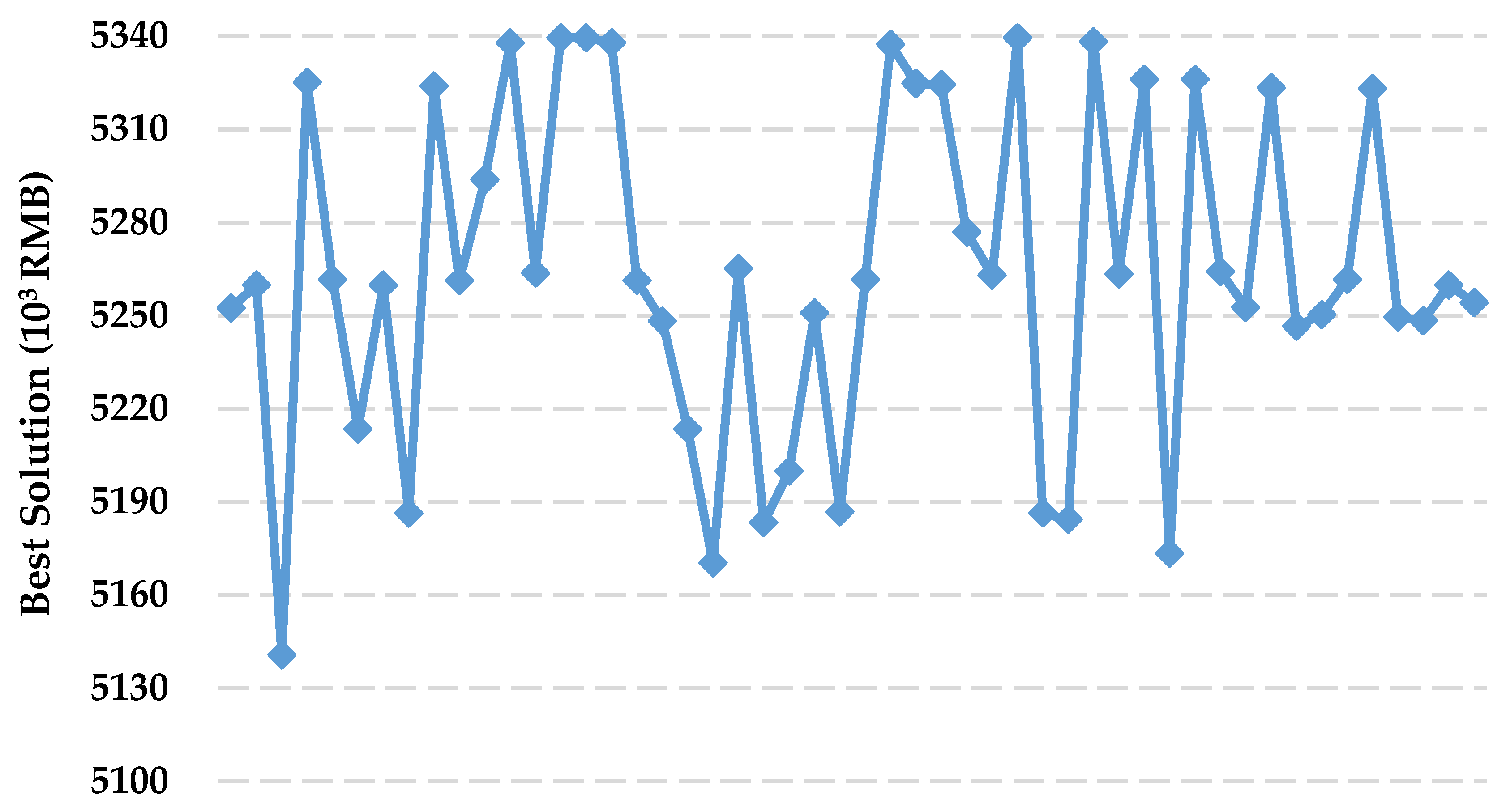
Next, we input the 50 sets of service capacities into the deterministic capacity constraint as in Equation (3), and generate actual best routes corresponding to each set of service capacities by using the MILP model established in our previous study. The statistics of the 50 best solutions (i.e., the minimal generalized costs) are presented in Figure 8. Based on the statistics, we can implement Step 2 in Table 3.
In this study, we use the root mean square (RMS) of the best solution to the intermodal routing decision with service capacity uncertainty with respect to the ones to the 50 simulation intermodal transportation scenarios in order to evaluate the gap between the planned best routes and the actual best ones. The calculation of the mean squared error is given in Equation (9):
where is the above RMS under confidence . is the total number of the fuzzy simulations, and in this study, = 50. is the index of the fuzzy simulation, and . is the best solution to the intermodal routing decision with service capacity uncertainty under confidence . is the best solution to the intermodal routing decision with deterministic service capacities that are generated in the gth fuzzy simulation. The comparison between the planned best routes under confidence = 0.9 and 1.0 is summarized in Table 5.
According to Table 4, we can implement Step 3 as follows. Honestly, as the authors of this paper, we prefer the first case if we were the decision makers.
- (1)
- If the decision makers prefer high reliability and would like to sacrifice transportation efficiency to some extent, the value of confidence can set to 1.0, because the feasible ratio can remarkably improve with a slight increase of the minimal generalized costs and the deviation to the practice.
- (2)
- If the decision makers attach more importance to transportation efficiency and accept a feasible ratio of 80%, the value of confidence can be set to 0.9.
5. Conclusions
In this study, we systematically explore how service capacity uncertainty influences intermodal decision-making. Such an exploration bridges the research gap in that there are rare intermodal routing decision studies that consider the service capacity uncertainty. The main work accomplished in this study is summarized as follows.
- (1)
- We adopt a fuzzy programming approach that is easily realized in transportation practice to formulate the service capacity uncertainty. Based on the fuzzy credibility measure, the deterministic service capacity constraint is improved to be a fuzzy chance constraint whose crisp equivalent linear reformulations can be effectively assessed.
- (2)
- We use a sensitivity analysis to indicate the influence of service capacity uncertainty programmed by the fuzzy chance constraint on the intermodal routing decision, and draw the conclusion that the transportation economy and transportation reliability cannot reach an optimum simultaneously, so a tradeoff between them should be made by the decision makers.
- (3)
- We employ fuzzy simulation to help decision makers to select a suitable confidence value during advanced decision-making to make an effective tradeoff between transportation economy and reliability.
The fuzzy programming framework, which comprehensively utilizes fuzzy chance constraint modeling, sensitivity analysis, and fuzzy simulation, provides a helpful response to the challenge proposed by the uncertainty issues in various planning problems. It can be promoted for routing problems in other research fields, e.g., wireless communications [28] and manufacturing systems [29], as well as other transportation planning problems, e.g., service network design [30,31], when there is a need to deal with uncertainty from a fuzzy programming perspective.
Acknowledgments
This study was supported by the National Social Science Foundation of China under Grant No. 17CGL019. The authors would also like to thank Cyril B. Lucas from the United Kingdom, author of the book Atomic and Molecular Beams: Production and Collimation, for helping us edit and polish the language of this paper.
Author Contributions
Yan Sun and Kunxiang Dong proposed the topic explored in this paper. Yan Sun, Guijie Zhang and Zhijuan Hong discussed and designed the fuzzy programming approach. Yan Sun and Guijie Zhang conducted the sensitivity analysis and fuzzy simulation in the case study. Yan Sun and Kunxiang Dong wrote the paper. Zhijuan Hong and Kunxiang Dong thoroughly reviewed and improved the paper. All authors have discussed and contributed to the manuscript. All authors have read and approved the final manuscript.
Conflicts of Interest
The authors declare no conflict of interest.
Appendix A

Table A1.
Fuzzy capacities of the transportation services.
| Road Services | Fuzzy Capacities | Road Services | Fuzzy Capacities |
| (1, 2) | 112, 123, 141, 162 | (20, 40) | 45, 60, 90, 105 |
| (1, 3) | 96, 123, 135, 153 | (22, 14) | 72, 93, 120, 132 |
| (1, 10) | 75, 90, 114, 135 | (22, 40) | 66, 84, 105, 132 |
| (2, 1) | 72, 87, 99, 120 | (22, 34) | 90, 120, 135, 180 |
| (2, 3) | 60, 75, 99, 118 | (22, 35) | 60, 72, 105, 120 |
| (2, 9) | 90, 120, 138, 159 | (22, 36) | 75, 84, 114, 141 |
| (3, 9) | 36, 75, 90, 120 | (22, 37) | 105, 120, 141, 150 |
| (3, 10) | 30, 42, 60, 72 | (22, 38) | 72, 84, 99, 120 |
| (3, 13) | 72, 96, 114, 135 | (23, 32) | 48, 54, 72, 90 |
| (4, 5) | 66, 84, 99, 111 | (24, 23) | 30, 36, 45, 60 |
| (4, 6) | 45, 75, 96, 108 | (24, 32) | 24, 48, 75, 90 |
| (4, 7) | 66, 84, 99, 114 | (25, 23) | 15, 48, 72, 96 |
| (4, 8) | 126, 150, 156, 186 | (25, 32) | 63, 72, 87, 105 |
| (4, 11) | 90, 138, 171, 180 | (26, 23) | 33, 51, 60, 75 |
| (4, 12) | 42, 63, 99, 126 | (26, 32) | 63, 72, 90, 99 |
| (4, 13) | 90, 111, 120, 138 | (27, 23) | 105, 123, 132, 150 |
| (4, 14) | 69, 96, 120, 135 | (27, 32) | 57, 72, 90, 120 |
| (4, 18) | 42, 60, 90, 114 | (28, 23) | 60, 78, 93, 117 |
| (8, 11) | 36, 54, 78, 93 | (28, 32) | 84, 90, 117, 126 |
| (8, 12) | 102, 120, 138, 156 | (29, 23) | 63, 84, 105, 132 |
| (8, 13) | 78, 93, 105, 129 | (29, 32) | 105, 120, 141, 162 |
| (9, 13) | 78, 108, 132, 150 | (30, 23) | 33, 51, 66, 78 |
| (9, 18) | 75, 93, 99, 114 | (30, 32) | 66, 78, 84, 123 |
| (10, 13) | 48, 84, 102, 120 | (31, 23) | 111, 120, 150, 180 |
| (10, 18) | 54, 75, 99, 123 | (31, 32) | 63, 102, 120, 144 |
| (13, 18) | 30, 51, 69, 96 | (32, 23) | 81, 102, 135, 165 |
| (14, 21) | 135, 168, 186, 204 | (33, 15) | 135, 150, 162, 183 |
| (14, 22) | 93, 132, 81, 105 | (33, 40) | 72, 123, 144, 159 |
| (14, 32) | 120, 138, 159, 171 | (33, 34) | 75, 96, 132, 171 |
| (15, 18) | 63, 90, 120, 135 | (33, 35) | 96, 129, 147, 177 |
| (15, 40) | 99, 108, 138, 153 | (33, 36) | 102, 147, 168, 180 |
| (16, 18) | 57, 78, 96, 129 | (33, 37) | 126, 150, 165, 183 |
| (16, 40) | 42, 66, 90, 120 | (33, 38) | 105, 120, 144, 159 |
| (17, 18) | 72, 81, 99, 132 | (39, 14) | 141, 168, 180, 195 |
| (17, 40) | 84, 108, 123, 141 | (39, 21) | 111, 132, 159, 186 |
| (18, 40) | 54, 75, 93, 108 | (39, 22) | 72, 108, 123, 156 |
| (19, 18) | 42, 75, 93, 120 | (39, 23) | 93, 114, 144, 165 |
| (19, 40) | 75, 105, 120, 150 | (39, 32) | 120, 138, 171, 186 |
| (20, 18) | 72, 84, 111, 120 | (40, 15) | 60, 75, 108, 135 |
| Railway Services | Fuzzy Capacities | Railway Services | Fuzzy Capacities |
| (1, 3) | 105, 132, 180, 210 | (14, 26) | 9, 18, 42, 60 |
| (2, 3) | 156, 183, 216, 234 | (14, 27) | 12, 30, 60, 72 |
| (5, 3) | 135, 150, 174, 195 | (14, 28) | 6, 12, 42, 54 |
| (6, 3) | 54, 90, 144, 156 | (21, 23) | 261, 300, 324, 345 |
| (7, 3) | 45, 60, 90, 114 | (21, 24) | 30, 42, 75, 90 |
| (8, 9) | 120, 150, 168, 180 | (21, 26) | 15, 24, 54, 81 |
| (8, 10) | 126, 165, 174, 198 | (21, 27) | 15, 30, 51, 60 |
| (11, 9) | 39, 66, 84, 96 | (21, 28) | 42, 60, 99, 120 |
| (11, 10) | 72, 84, 171, 201 | (22, 24) | 18, 24, 42, 57 |
| (11, 13) | 81, 120, 144, 171 | (22, 25) | 15, 30, 60, 90 |
| (12, 9) | 24, 60, 105, 120 | (22, 26) | 6, 18, 45, 63 |
| (12, 10) | 42, 60, 78, 90 | (22, 28) | 15, 24, 42, 60 |
| (12, 13) | 156, 180, 216, 228 | (22, 29) | 6, 12, 33, 54 |
| (14, 15) | 30, 48, 69, 87 | (22, 30) | 27, 36, 66, 78 |
| (14, 16) | 18, 30, 60, 72 | (22, 31) | 36, 48, 84, 99 |
| (14, 17) | 45, 66, 84, 93 | (22, 32) | 90, 108, 156, 189 |
| (14, 18) | 99, 126, 168, 177 | (34, 40) | 30, 42, 60, 75 |
| (14, 19) | 12, 30, 69, 84 | (35, 40) | 33, 48, 63, 90 |
| (14, 20) | 6, 15, 42, 54 | (36, 40) | 24, 30, 57, 66 |
| (14, 23) | 222, 300, 342, 360 | (37, 40) | 21, 36, 54, 78 |
| (14, 24) | 63, 84, 120, 129 | (38, 40) | 120, 144, 165, 183 |
References
- Janic, M. Modelling the full costs of an intermodal and road freight transport network. Transp. Res. Part D Transp. Environ. 2007, 12, 33–44. [Google Scholar] [CrossRef]
- Liao, C.H.; Tseng, P.H.; Lu, C.S. Comparing carbon dioxide emissions of trucking and intermodal container transport in Taiwan. Transp. Res. Part D Transp. Environ. 2009, 14, 493–496. [Google Scholar] [CrossRef]
- Sun, Y.; Lang, M.X.; Wang, D.Z. Optimization models and solution algorithms for freight routing problem in the multimodal transportation networks: A review of the state-of-the art. Open Civ. Eng. J. 2015, 9, 714–723. [Google Scholar] [CrossRef]
- Ziliaskopoulos, A.; Wardell, W. An intermodal optimum path algorithm for multimodal networks with dynamic arc travel times and switching delays. Eur. J. Oper. Res. 2000, 125, 486–502. [Google Scholar] [CrossRef]
- Lam, S.K.; Srikanthan, T. Accelerating the K-shortest paths computation in multimodal transportation networks. In Proceedings of the IEEE 5th International Conference on Intelligent Transportation Systems, Singapore, 6 September 2002; pp. 491–495. [Google Scholar]
- Boussedjra, M.; Bloch, C.; El Moudni, A. An exact method to find the intermodal shortest path (ISP). In Proceedings of the 2004 IEEE International Conference on Networking, Sensing and Control, Taipei, Taiwan, 21–23 March 2004; pp. 1075–1080. [Google Scholar]
- Xiong, G.; Wang, Y. Best routes selection in multimodal networks using multi-objective genetic algorithm. J. Comb. Optim. 2014, 28, 655–673. [Google Scholar] [CrossRef]
- Sun, B.; Chen, Q. The routing optimization for multi-modal transport with carbon emission consideration under uncertainty. In Proceedings of the 32nd Chinese Control Conference (CCC), Xi’an, China, 26–28 July 2013; pp. 8135–8140. [Google Scholar]
- Chang, T.S. Best routes selection in international intermodal networks. Comput. Oper. Res. 2008, 35, 2877–2891. [Google Scholar] [CrossRef]
- Sun, H.; Li, X.; Chen, D. Modeling and solution methods for viable routes in multimodal networks. In Proceedings of the 4th IEEE International Conference on Management of Innovation and Technology, Bangkok, Thailand, 21–24 September 2008; pp. 1384–1388. [Google Scholar]
- Kim, H.J.; Chang, Y.T.; Lee, P.T.W.; Shin, S.H.; Kim, M.J. Optimizing the transportation of international container cargoes in Korea. Marit. Policy Manag. 2008, 35, 103–122. [Google Scholar] [CrossRef]
- Ayar, B.; Yaman, H. An intermodal multicommodity routing problem with scheduled services. Comput. Optim. Appl. 2012, 53, 131–153. [Google Scholar] [CrossRef]
- Moccia, L.; Cordeau, J.F.; Laporte, G.; Ropke, S.; Valentini, M.P. Modeling and solving a multimodal transportation problem with flexible-time and scheduled services. Networks 2011, 57, 53–68. [Google Scholar] [CrossRef]
- Lei, K.; Zhu, X.; Hou, J.; Huang, W. Decision of multimodal transportation scheme based on swarm intelligence. Math. Probl. Eng. 2014, 2014, 932832. [Google Scholar] [CrossRef] [PubMed]
- Sun, Y.; Lang, M.X. Modeling the multicommodity multimodal routing problem with schedule-based services and carbon dioxide emission costs. Math. Probl. Eng. 2015, 2015, 406218. [Google Scholar] [CrossRef]
- Sun, Y.; Lang, M.X. Bi-objective optimization for multi-modal transportation routing planning problem based on Pareto optimality. J. Ind. Eng. Manag. 2015, 8, 1195–1217. [Google Scholar] [CrossRef]
- Sun, Y.; Lang, M.X.; Wang, D.Z. Bi-objective modelling for hazardous materials road–rail multimodal routing problem with railway schedule-based space–time constraints. Int. J. Environ. Res. Public Health 2016, 13, 762. [Google Scholar] [CrossRef] [PubMed]
- Sun, Y.; Lang, M.; Wang, J. On Solving the Fuzzy Customer Information Problem in Multicommodity Multimodal Routing with Schedule-Based Services. Information 2016, 7, 13. [Google Scholar] [CrossRef]
- Liu, Q.; Xu, J. A study on vehicle routing problem in the delivery of fresh agricultural products under random fuzzy. Int. J. Inf. Manag. Sci. 2008, 19, 673–690. [Google Scholar] [CrossRef]
- Lium, A.G.; Crainic, T.G.; Wallace, S.W. A study of demand stochasticity in service network design. Transp. Sci. 2009, 43, 144–157. [Google Scholar] [CrossRef]
- Ji, X. Models and algorithm for stochastic shortest path problem. Appl. Math. Comput. 2005, 170, 503–514. [Google Scholar] [CrossRef]
- Ji, X.; Iwamura, K.; Shao, Z. New models for shortest path problem with fuzzy arc lengths. Appl. Math. Model. 2007, 31, 259–269. [Google Scholar] [CrossRef]
- Zarandi, M.H.F.; Hemmati, A.; Davari, S. The multi-depot capacitated location-routing problem with fuzzy travel times. Expert Syst. Appl. 2008, 38, 10075–10084. [Google Scholar] [CrossRef]
- López-Castro, L.F.; Montoya-Torres, J.R. Vehicle routing with fuzzy time windows using a genetic algorithm. In Proceedings of the 2011 IEEE Workshop on Computational Intelligence in Production and Logistics Systems (CIPLS), Paris, France, 11–15 April 2011; pp. 1–8. [Google Scholar]
- Zheng, Y.; Liu, B. Fuzzy vehicle routing model with credibility measure and its hybrid intelligent algorithm. Appl. Math. Comput. 2006, 176, 673–683. [Google Scholar] [CrossRef]
- Liu, B.; Iwamura, K. Chance constrained programming with fuzzy parameters. Fuzzy Sets Syst. 1998, 94, 227–237. [Google Scholar] [CrossRef]
- Schrage, L. LINGO User’s Guide; LINDO System Inc.: Chicago, IL, USA, 2006; Available online: http://www.lindo.com/ (accessed on 22 January 2018).
- Radi, M.; Dezfouli, B.; Bakar, K.A.; Lee, M. Multipath Routing in Wireless Sensor Networks: Survey and Research Challenges. Sensors 2012, 12, 650–685. [Google Scholar] [CrossRef] [PubMed]
- Joseph, O.A.; Sridharan, R. Analysis of dynamic due-date assignment models in a flexible manufacturing system. J. Manuf. Syst. 2011, 30, 28–40. [Google Scholar] [CrossRef]
- Crainic, T.G. Service network design in freight transportation. Eur. J. Oper. Res. 2000, 122, 272–288. [Google Scholar] [CrossRef]
- Qu, Y.; Bektaş, T.; Bennell, J. Sustainability SI: multimode multicommodity network design model for intermodal freight transportation with transfer and emission costs. Netw. Spat. Econ. 2016, 16, 303–329. [Google Scholar] [CrossRef]
Figure 1.
Possible consequence of the optimistic estimation.
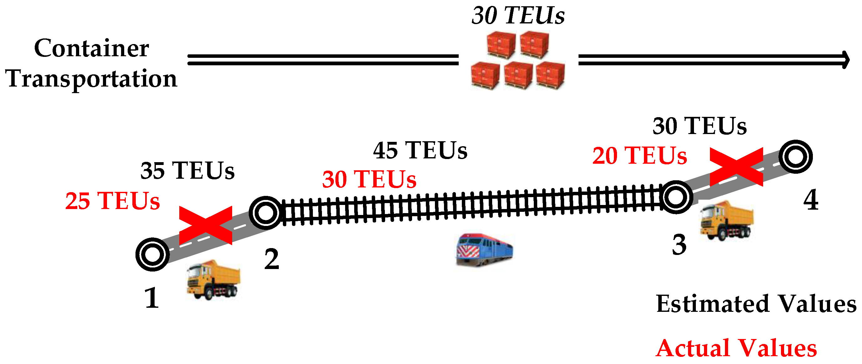
Figure 2.
Possible consequences of the pessimistic estimation.
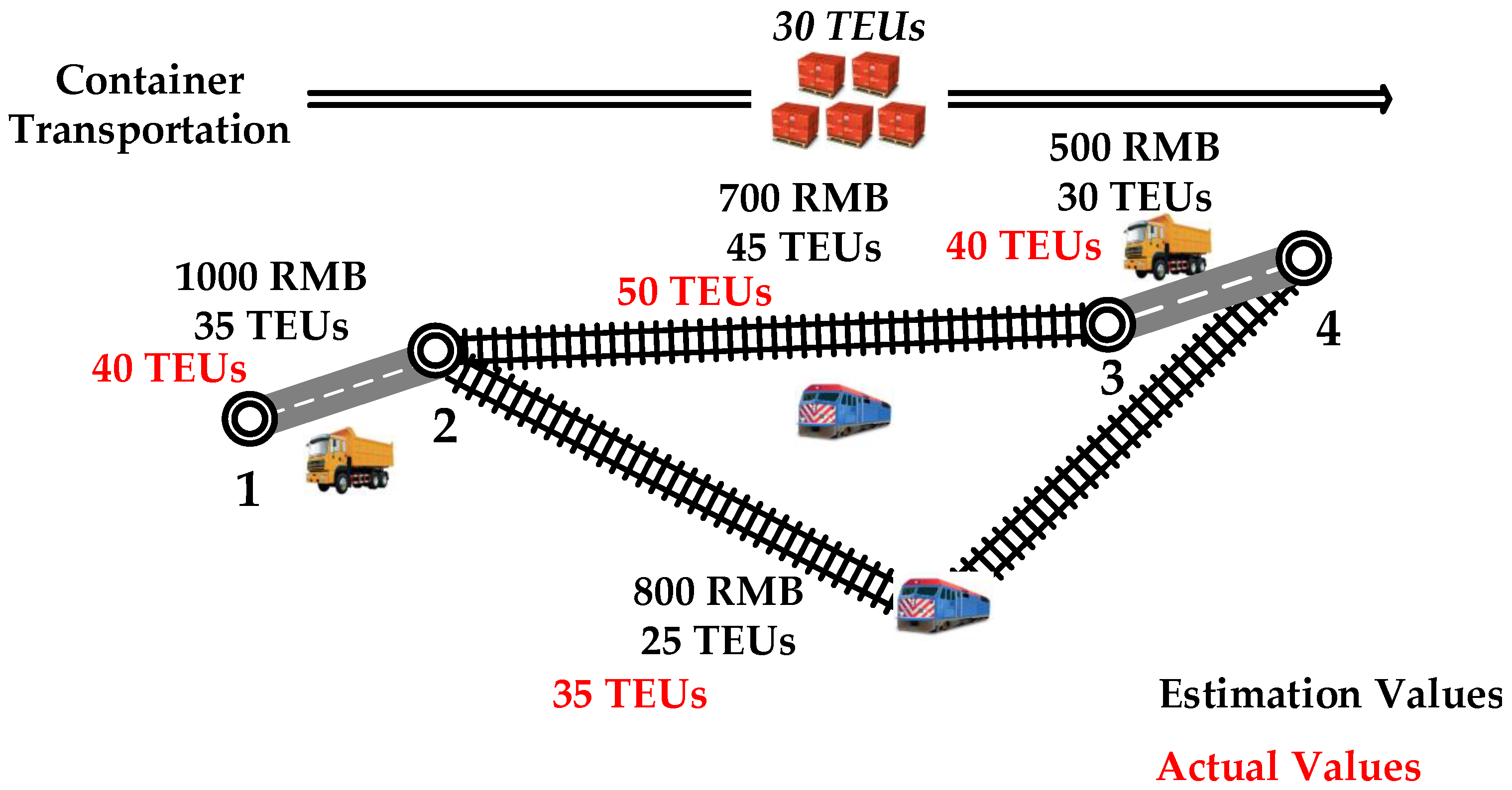
Figure 3.
Representations of the fuzzy service capacity, (a) by triangular fuzzy number; (b) by trapezoidal fuzzy number.
Figure 3.
Representations of the fuzzy service capacity, (a) by triangular fuzzy number; (b) by trapezoidal fuzzy number.

Figure 4.
Piecewise linear relationship in the credibility measure.

Figure 5.
Sensitivity of the intermodal routing with respect to the confidence value.
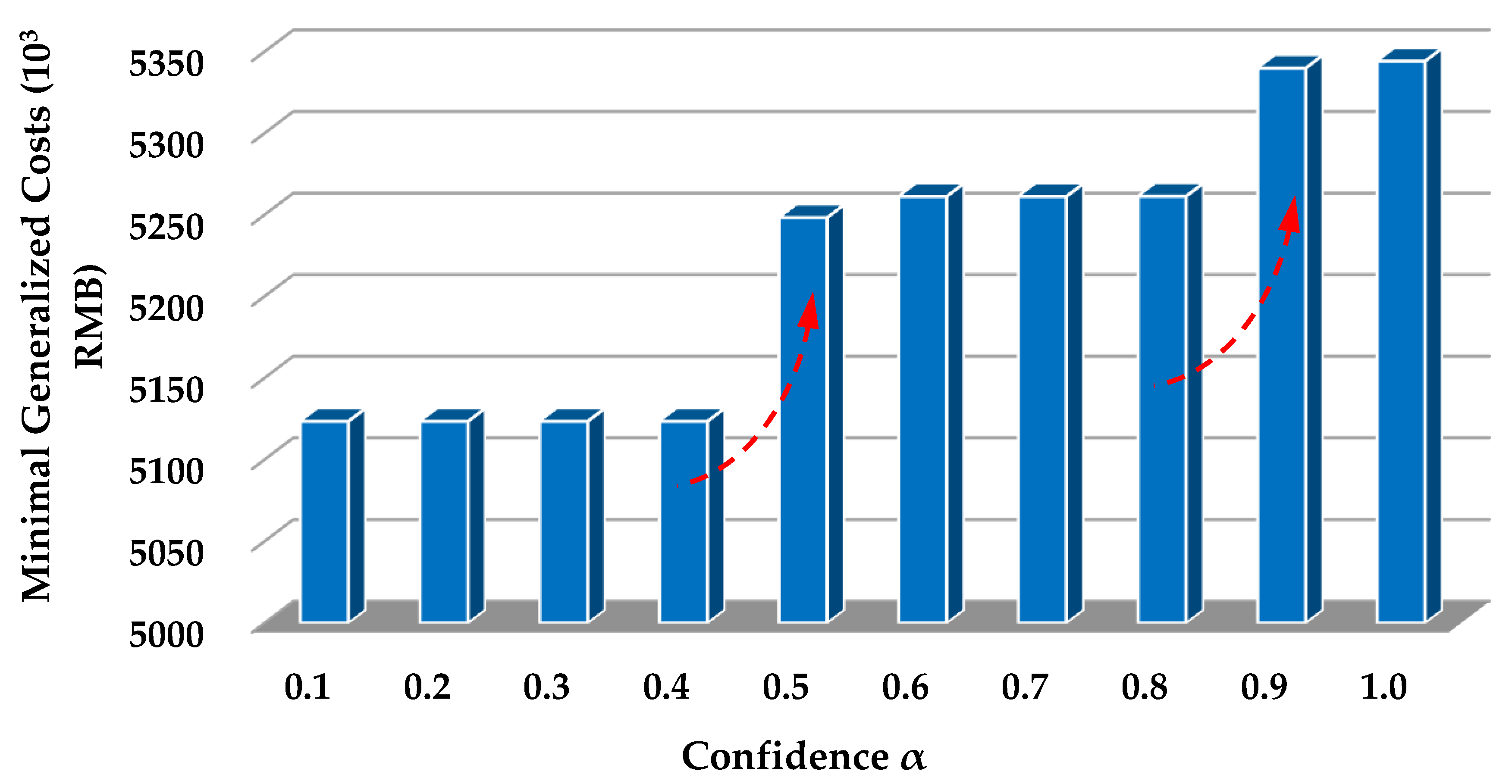
Figure 6.
Fuzzy simulation process.

Figure 7.
Fuzzy simulation results.

Figure 8.
Best solutions to the 50 simulated actual intermodal transportation scenarios.

Table 1.
Scale of the empirical case.
| Variables | 0–1 Variables | Constraints |
|---|---|---|
| 10,375 | 5675 | 36,028 |
Table 2.
Optimization results when confidence is 0.9.
| Algorithm | Best Solution | Solution State | Computational Time |
|---|---|---|---|
| Branch-and-Bound Algorithm | 5,339,867 RMB | Global Optimum | 95 s * |
* Average value of 10 simulations.
Table 3.
Procedure of evaluating the confidence values.
| Step 1 | Check whether the planned routes violate the actual capacities of the transportation services on them. If any one of the capacities is violated, the routing decision has failed (i.e., failed decision); otherwise, it is feasible (i.e., a feasible decision). |
| Step 2 | Compare the planned best routes with the actual best ones to evaluate their gaps. The smaller the gap, the better the feasibility of the planned routes. |
| Step 3 | Determine the best confidence value under consideration of the decision makers’ preference. |
Table 4.
Results of the intermodal routing decisions under three deterministic capacity scenarios.
| Optimization Results | Lower Bound Scenario | Median Value Scenario | Upper Bound Scenario |
|---|---|---|---|
| Best solutions | 5,245,192 RMB | 5,168,634 RMB | 5,123,383 RMB |
| Feasible ratios | 0% | 0% | 0% |
Table 5.
Comparison between the planned best routes under confidence = 0.9 and 1.0.
| Confidence Values | Best Solutions | Feasible Ratios | RMSs |
|---|---|---|---|
| 0.9 | 5,339,867 RMB | 80% | 92,306 RMB |
| 1.0 | 5,344,147 RMB | 100% | 95,824 RMB |
| GAP * | 0.08% | 25% | 3.8% |
* [(value corresponding to 1.0 − value corresponding to 0.9)/value corresponding to 0.9] × 100%.
© 2018 by the authors. Licensee MDPI, Basel, Switzerland. This article is an open access article distributed under the terms and conditions of the Creative Commons Attribution (CC BY) license (http://creativecommons.org/licenses/by/4.0/).
Share and Cite
MDPI and ACS Style
Sun, Y.; Zhang, G.; Hong, Z.; Dong, K. How Uncertain Information on Service Capacity Influences the Intermodal Routing Decision: A Fuzzy Programming Perspective. Information 2018, 9, 24. https://doi.org/10.3390/info9010024
AMA Style
Sun Y, Zhang G, Hong Z, Dong K. How Uncertain Information on Service Capacity Influences the Intermodal Routing Decision: A Fuzzy Programming Perspective. Information. 2018; 9(1):24. https://doi.org/10.3390/info9010024
Chicago/Turabian StyleSun, Yan, Guijie Zhang, Zhijuan Hong, and Kunxiang Dong. 2018. "How Uncertain Information on Service Capacity Influences the Intermodal Routing Decision: A Fuzzy Programming Perspective" Information 9, no. 1: 24. https://doi.org/10.3390/info9010024
Note that from the first issue of 2016, this journal uses article numbers instead of page numbers. See further details here.